Trivariate Simplex Splines for Inhomogeneous SolidModeling in Engineering Design

Jing Hua∗, Ying He†, and Hong Qin†∗Computer Science, Wayne State University†Computer Science, Stony Brook University

Abstract

This paper presents a new inhomogeneous solid modeling paradigm for engineering design. The proposed paradigmcan represent, model, and render multi-dimensional, physical attributes across any volumetric objects of complicatedgeometry and topology. A modeled object is formulated with a trivariate simplex spline defined over a tetrahedral decom-position of its 3D domain. Heterogeneous material attributes associated with solid geometry can be easily modeled andedited by manipulating the control vectors and/or associated knots of trivariate simplex splines. We also develop a feature-sensitive fitting algorithm that can reconstruct a compact, continuous trivariate simplex spline from measured, structuredor unstructured volumetric grids of real-world inhomogeneous objects. In addition, we propose a fast direct renderingalgorithm for interactive data analysis and visualization of the simplex spline volumes. Our experiments demonstrate thatthe proposed paradigm augments the current engineering design techniques with the new and unique advantages.

List of Figures

1 Volume rendering of 10 quadratic DMS-spline basis functions. . . . . . . . . . . . . . . . . . . . . . . . 42 (a) A cubic trivariate DMS-spline solid corresponding to a single tetrahedral domain with 20 control points.

(b) The tetrahedra of the designed solid object are scaled to show the interior of the solid. . . . . . . . . . 53 A DMS-spline solid object corresponding to the tetrahedral domain. (a) A domain tetrahedralization. (b)

Volume rendering of the resulting solid model which is genus-20. . . . . . . . . . . . . . . . . . . . . . 64 (a) The piecewise linear boundary constraints that the user specifies. (b) The multiresolution tetrahedraliza-

tion conforming to the piecewise linear boundary constraints. (c) The color map of material distribution ofthe designed object. (d) Volume rendering of the designed object, where we can see that all the geometricshape features are preserved. . . . . . . . . . . . . . . . . . . . . . . . . . . . . . . . . . . . . . . . . . 7

5 (a) The tetrahedral domain of a geometrically smooth object. (b) Volume rendering of the designed object,where we can see the density discontinuities shown in different colors. . . . . . . . . . . . . . . . . . . . 8

6 (a) The point view of the spx dataset, where the color indicates the density difference. (b) Occupancy mapof the point set. (c) The final tetrahedralization after removing the outside tetrahedra. . . . . . . . . . . . 9

7 (a) Geometric features of the spx dataset. (b) The finally constructed initial tetrahedralization. . . . . . . 108 The fitting results for the spx dataset. (a)-(b) Fitting with control vectors only (front view and side view).

(c)-(d) Fitting with both control vectors and knots (front view and side view). . . . . . . . . . . . . . . . 129 Simplex spline based fitting examples. . . . . . . . . . . . . . . . . . . . . . . . . . . . . . . . . . . . . 12

List of Tables

1 Statistics of Data fitting. . . . . . . . . . . . . . . . . . . . . . . . . . . . . . . . . . . . . . . . . . . . 14

1

1 Introduction and Motivation

Real-world objects are active, responsive, and anisotropic. Oftentimes, they are of arbitrary topology and complex geom-etry. The fundamental objectives in engineering design are to unambiguously model physical volumetric objects, inter-actively visualize their geometric and physical attribute properties, and rigorously analyze their kinematic and dynamicnatures. With the advent of ever-increasing computing power and more advanced data acquisition technologies, solidgeometry has quickly gained popularity as an intuitive and natural paradigm for these purposes. New and powerful solidrepresentations underpin the success of solid modeling and relevant applications. To date, the vast majority of popular solidmodeling approaches, as well as commonly-used solid modeling systems, are built upon the following geometric founda-tions: constructive solid geometry (CSG), boundary representation (B-reps), and cell decomposition. When our goals areto reconstruct heterogeneous models of physical objects with continuous properties, and further model and visualize theobjects, prior representations and the current state-of-the-art in engineering design fall short in offering designers an inte-grated paradigm to represent complex solid geometry, arbitrary topology, and continuously-varying material attributes in asingle framework simultaneously.

To model heterogeneous volumetric objects with high-order continuity, techniques based on splines such as B-splinesor NURBS [1, 2, 3, 4] are frequently used. Nonetheless, modeling with B-splines or NURBS has severe shortcomings.Its modeling scope is extremely constrained in term of geometric, topological, and attribute aspects. First, B-spline andNURBS are defined over a regular, tensor-product domain. A single B-spline or NURBS cannot represent volumes ofcomplex topology without patching or trimming operations. Furthermore, patching multiple B-splines or NURBS to formcomplex topology is not easy to control at all. Second, tensor-product splines are essentially smooth everywhere. It isdifficult to model high-frequency features. Third, when refining a region of interest in a tensor-product spline patch, it willintroduce too many extra degrees of freedom in other less interesting regions nearby in order to retain its regular structure.Attractive properties such as local adaptivity and multiresolution are rather difficult to achieve.

To overcome the above difficulties, we propose an integrated approach for representing, modeling, and rendering ofmulti-dimensional, physical attributes across any volumetric object. Our goal is to demonstrate that the trivariate simplexspline is a promising primitive for both visualization and modeling in engineering design tasks, especially for representingand visualizing heterogeneous models of physical objects and their material properties. Our model makes use of a moregeneral and flexible tetrahedral domain and offers a compact, continuous representation because it is a piecewise poly-nomial of the lowest possible degree and the highest possible continuity everywhere across the entire tetrahedral domain.It unifies geometry and attribute properties over domains of complex topology. It is possible to represent a complicatedheterogeneous object with a single trivariate simplex spline without any additional operations of trimming or patching,while the geometry of the object is explicitly represented by the spline. For example, given a degreen for the trivariteDMS-spline [5] which uses simplex spline as basis functions, the representation scheme can achieveCn−1 continuity oversmooth regions. Meanwhile, by placing control points and their associated knots in certain locations, variable continuity isreadily accomplished including aC0 continuity that defines sharp features. This property is ideal for data reduction whenreverse-engineering a continuous spline model from the discretized data inputs.

Since we develop the trivariate simplex spline for both solid geometry and the material attributes associated with thesolid geometry simultaneously, it facilitates the modeling of heterogeneous objects. The feature-sensitive fitting algorithmthat we develop can reconstruct a more compact trivariate simplex spline from a structured or arbitrary unstructured volumemeasured from the real world. It reconstructs the geometry and the associated material attributes simultaneously. TheCn−1 continuity andC0 continuity can both be modeled with ease using simplex splines. Such flexibility allows us tomodel continuously-varying material distribution. It may be noted that, in our framework we use time-varying knotsinstead of fixed knots, which offer more freedom and improves accuracy for approximation. The knots are explicitlyand automatically determined by optimizing a specific objective function. This representation can also enable the strongmultiresolution modeling capability through interactively subdividing any region of interest, allocating more knots andcontrol points accordingly. In addition, we propose a fast direct rendering algorithm for interactive data analysis andvisualization of the simplex spline volumes. When visualizing this type of solids, resampling or interpolation process isno longer necessary at all. It (including position, derivative, etc.) can be evaluated anywhere analytically and computedefficiently for volume rendering.

1.1 Related Work

Research on volume modeling using B-splines or NURBS has received much attention in the modeling community in recentyears. Raviv and Elber [1] presented a 3D interactive sculpting paradigm that employed a set of scalar uniform trivariate B-

2

spline functions as object representations. Schmitt and Pasko [3] presented an approach for constructive modeling of FRepsolids defined by real-valued functions using 4D uniform rational cubic B-spline volumes as primitives. Hua and Qin [2]presented a haptics-based direct manipulation and exploration of scalar B-spline volumes. Martin and Cohen [4] presenteda completed mathematical framework for representing and extracting volumetric attributes using trivariate NURBS.

Multivariate simplex splines for approximation theory have been extensively investigated in mathematical science formany years. Motivated by an idea of Curry and Schoenberg for a geometric interpretation of univariate B-splines, deBoor [6] first presented a brief description of multivariate simplex splines. Since then, their theoretical aspects havebeen explored extensively. From the point of view of blossoming, Dahmenet. al [5] proposed triangular B-splines. Incontrast to the theoretical advances, the application of multivariate simplex splines has been under-explored. Greiner andSeidel [7] demonstrated the practical feasibility of multivariate B-spline algorithms in graphics and shape design. Pfeifleand Seidel proposed a fast evaluation technique for quadratic bivariate DMS-spline surfaces [8] and demonstrated the fittingof triangular B-spline surfaces to scattered data through the use of least squares and optimization techniques [9]. Qin andTerzopoulos [10] presented dynamic triangular NURBS, a free-form shape model. He and Qin [11] presented an approachfor reconstructing a triangular B-spline surface from a set of scanned 3D points. To the authors’ best knowledge, there areno existing research work, which applies multivariate simplex splines to represent solid geometry, model its heterogeneousmaterial attributes, and reconstruct continuous volumetric splines from discretized volumetric inputs via data fitting.

2 Trivariate DMS-spline Volumes

Analogous to a tensor-product, trivariate B-spline volume [1, 4], we can instead use simplex splines to model volumetricobjects. To motivate our rationales, we have detailed some major advantages of multivariate simplex spline volumes overconventional tensor-product B-spline volumes in Section 1.

2.1 Trivariate Simplex Splines

Throughout this paper, we employ a trivariate simplex spline to represent and extract both solid geometry and its volumetricattributes. Now we shall review the formulation of the trivariate simplex splines and summarize their analytic and geometricproperties.

A degreen trivariate simplex spline,M(u|u0, · · · ,un+3), can be defined as a function ofu ∈ R3 over the half openconvex hull of a point setV = [u0, · · · ,un+3), depending on then+4 knotsui ∈ R3, i = 0, · · · ,n+3. The basis function oftrivariate simplex splines may be formulated recursively, which facilitates point evaluation and its derivative and gradientcomputation. Whenn = 0,

M(u|u0, · · · ,u3) =

1

|VolR3(u0,···,u3)| , u ∈ [u0, · · · ,u3),

0, otherwise,

and whenn > 0, select four pointsW = uk0,uk1,uk2,uk3 from V, such thatW is affinely independent, then

M(u|u0, · · · ,un+3) =3

∑j=0

λ j(u|W)M(u|V \uk j), (1)

where∑3j=0 λ j(u|W) = 1 and∑3

j=0 λ j(u|W)uk j = u.The directional derivative ofM(u|V) with respect to a vectorv is defined as follows:

DvM(u|V) = n3

∑j=0

µj(v|W)M(u|V \uk j), (2)

wherev = ∑3j=0µj(v|W)uk j and∑3

j=0µj(v|W) = 0. In the interest of conserving space, we leave more theoretical discus-sions to other treatments of simplex splines in the references and elsewhere.

2.2 Trivariate DMS-spline Volumes

In [5], Dahmen, Micchelli and Seidel presented a multivariate B-spline scheme, called DMS-spline, based on blendingfunctions and control vectors. The surface scheme is also called triangular B-spline, which has been studied in [7, 8, 9,10, 12].

3

We apply the trivariate DMS-spline to represent both solid geometry and its associated physical attributes in engineeringdesign. To the authors’ best knowledge, we pioneer the use of trivariate DMS-spline in solid modeling and visualization.Let Ω be an arbitrary proper tetrahedralization ofR3 or some bounded domainD ⊂ R3. Here, “Proper” means that everypair of domain tetrahedra are disjoint, or share exactly one vertex, one edge, or one face.

To each vertext of the tetrahedralization, we assign a knot cloud, which is a sequence of points[t0, t1, · · · , tn], wheret0 ≡ t. For every tetrahedronI = (p,q, r ,s), we require

• all the tetrahedra[pi ,q j , rk,sl ] with i + j +k+ l ≤ n are non-degenerate.

• the setinterior(∩i+ j+k+l≤n[pi ,q j , rk,sl ]) 6= ∅. (3)

• if I has a boundary triangle, the knots associated to the boundary triangle must lie outside ofΩ.

We then define, for each tetrahedronI andi + j +k+ l = n (in the following, we useβ to denote 4-tuple(i, j,k, l)), theknot sets

V Iβ = [p0, · · · ,pi ,q0, · · · ,q j , r0, · · · , r k,s0, · · · ,sl ]. (4)

The basis functions of normalized simplex splines are then defined as

NIβ(u) = |d(pi ,q j , rk,sl )|M(u|V I

β), (5)

where|d(pi ,q j , r k,sl )| is six times of the volume of(pi ,q j , r k,sl ). Like the ordinary tensor-product B-spline, a trivariatesimplex spline volume of degreen over arbitrary tetrahedral domain is the combination of a set of basis functions withcontrol vectorscI

β:

s(u) = ∑I∈Ω

∑|β|=n

cIβNI

β(u). (6)

Like B-splines, the nonnegative basis functions of simplex spline volume can be normalized to sum to unity. Theyhave a number of nice properties, such as the convex hull property, local support, affine invariance. Shape design based ontrivariate DMS-spline volume includes the specification of a domain tetrahedralization, knot sequences, and control pointsto generate an initial shape. The initial shape is then refined into the final desired shape through interactive adjustment ofdomain tetrahedralization, control points, and knots. The geometric flexibility of simplex spline volumes provides greatpower on its shape editing. Figure 1 shows the volume rendering of 10 quadratic DMS-spline basis functions, where thenumbers are 4-tuples of vertices of a knot tetrahedron. Figure 2(a) shows a cubic trivariate DMS-spline solid correspondingto a domain with a single tetrahedron. Note that our trivariate DMS volumes represent not only boundary geometry, butalso interior solid geometry. They can represent physical or material attributes over the entire solid as well. Figure 2(b)shows scaled tetrahedra of the solid in order to emphasize its non-empty solid interior geometry.

0002 0020 2000 0200 0011 0110 1100 1010 1001 0101

Figure 1: Volume rendering of 10 quadratic DMS-spline basis functions.

For a general trivariate DMS-spline volume, each domain tetrahedronI has its own set of control pointscIβ. However,

in this paper, we consider a more restricted class of volumes by sharing respective control points along common trianglesof two adjacent tetrahedra in parametric tetrahedralization. Splines with shared control points have a direct visual effect ingeometric and solid modeling. More importantly, as proved by Dahmen et. al [5], a degreen trivariate DMS-spline withshared control points can be evaluated with the efficiency of a degreen−1 spline.

s(u) = ∑I∈Ω

∑|β|=n−1

cIβ(u)NI

β(u)

wherecIβ(u) = ∑3

m=0cIβ+emλm(u|pi ,q j , rk,sl ) andem = (δi,m)3

i=0, m= 0,1,2 as the coordinate vectors.

4

(a) (b)

Figure 2: (a) A cubic trivariate DMS-spline solid corresponding to a single tetrahedral domain with 20 control points. (b)The tetrahedra of the designed solid object are scaled to show the interior of the solid.

This property can significantly improve the software system for rendering a DMS-spline volume. It also implies thatthe knotst i,n|i ∈ N have no effect on the value ofs(u).

Note that for our trivariate DMS-spline volumes, the used tetrahedral domain does not need to undergo a separate para-meterization process, because it is already conforming to the 3D physical domain for material attributes. Thegeneralizedcontrol vectors are now(n+3) vectors, including control points(px, py, pz) for the solid geometry, and control coefficients(g1, · · · ,gn) for the attributes, wheren denotes the number of attributes associated with the geometry.

2.3 Coupling Solid Geometry and Physical Attributes

In our framework, we consider that a control coefficient (and possibly other vector-based quantities withn components) isassociated with a corresponding control point and evaluated with the geometry simultaneously based on the same tetrahe-dral domain. In this way, we shall generalize DMS-spline technique from geometric domains to visual or material domains.Typical material-oriented examples include: mass, damping, stiffness (such as strain and stress), and displacement for solidphysics; or density, velocity, and pressure for fluid mechanics, etc. These attributes may be assigned at the control points orfitted by using both control vectors and knots. Other commonly-used visual information include: color, texture, intensity,opacity, transparency, etc. This flexibility permits our paradigm to be employed in a wide variety of applications involvingcontinuous domains, such as finite element analysis, virtual sculpting, and computational fluid simulation.

Consider that control coefficientsgIβ are associated with control pointspI

β (gIβ may be a multi-dimensional vector).

Besides solid geometry, a material (e.g., density) function overs(u) can be simultaneously defined as[gs

](u) = ∑

i

[gI

βpI

β

]NI

β(u), (7)

whereg can be color, texture, mass, temperature, or other visual or material functions as stated above. Visual and materialmodeling is indispensable for computerized virtual environments. Besides commonly-used material distributions in clas-sical mechanics, it can be generalized to heat transfer, electricity, and beyond. The diverse set of these novel solid modelsare very powerful because they can potentially unify geometric, topological, kinematic, material, and dynamic properties.

The field attributes can be modified by directly changing the control coefficients stored at the control points. In addition,by moving the control points, we can perform free form deformation (FFD) of the underlying geometric space. As a result,this procedure deforms the field properties and provides an alternate interaction mechanism. The geometric space overwhich the field is defined can be of very complicated topology, which adds further shape editing flexibility.

3 Multiresolution Modeling

Based on the flexible simplex splines, we can readily achieve multiresolution modeling of heterogeneous solid objects.The multiresolution capability is achieved by interactively subdividing any region of interest and allocating more knots andcontrol vectors accordingly.

3.1 Interactive Tetrahedralization

We use Delaunay tetrahedralization to construct a tetrahedral domain, which serves as the tetrahedral domain of the trivari-ate simplex spline.

5

For constructing Delaunay tetrahedralization for a 3D point set, we make use of the incremental flip algorithm proposedin [13, 14]. The procedure to update a tetrahedralization is to insert one new vertex at each step. Then, a sequence ofactions are applied to modify the tetrahedralization locally. Each flip action consists of replacing one, two, or three adjacenttetrahedra with four, three, or two new tetrahedra, respectively. When the new vertex lies either on a triangular face or onan edge of the current tetrahedralization, other face flips may be needed. When performing Delaunay tetrahedralization,the user have an option to enforce the quality constraints (including volume of tetrahedron, etc.).

The user can also interactively specify boundary constraints (such as points, edges, polygons, or cells). We implementthe boundary conforming Delaunay tetrahedralization [15], which tries to recover the missing boundary edges of thepiecewise linear complexes from its current Delaunay tetrahedralization by inserting new points.

3.2 Geometric Editing Using Control Points

With this flexible modeling technique, we can straightforwardly design solid geometric shapes with sharp features andassociated high frequency material properties. Since the control vectors include the position of control points and associatedcontrol coefficients, editing of control points and/or control coefficients offer more powerful modeling capabilities. Movingcontrol points around can directly lead to a desired deformation of the underlying model easily. Usually when the numberof control points is very large, it is tedious and relatively difficult to manipulate the control points individually. In oursystem we provide Free-Form Deformation (FFD) tools to allow users to move control points.

Based on our experiments, we observe that associating control points to a domain in such a way: locating control pointsat the edges of tetrahedra of the domain, can well preserve the shape and features represented by the original domain. Thedifference between the geometry of the domain and the resulting DMS solid object is very small. For example, for a DMS-spline of degreen, we place control points on all the vertices of its domain tetrahedra. In addition, we placen−1 controlpoints on each edge of the domain tetrahedra, which divide the edge ton equal-length line segments. Figure 3 shows anillustration. Figure 3(a) is a tetrahedral domain. After associating control points as described above, the correspondingDMS-spline solid object can be evaluated as shown in Fig. 3(b). The resulting solid model exhibits very complex topology,which is genus-20.

(a) (b)

Figure 3: A DMS-spline solid object corresponding to the tetrahedral domain. (a) A domain tetrahedralization. (b) Volumerendering of the resulting solid model which is genus-20.

Figure 4 shows another example. The user first builds a 3D piecewise linear complex as shown in Fig. 4(a), then oursystem generates its quality conforming Delaunay mesh. Badly shaped elements from the mesh are eliminated and replacedwith well shaped ones. This is done by automatically inserting additional points into current mesh. From Fig. 4(b), wecan see that more knots are generated around feature edges. By associating control points with the defined domain, all thefeatures are preserved in the resulting DMS solid of degree 4. Please refer to Fig. 4(d).

3.3 Attribute Editing Using Control Coefficients or Control Points

Besides modeling solid geometry, the user can easily edit associated physical or material attributes as well. This is achievedby editing control coefficients at the corresponding control points, because the underlying material distribution is in fact atrivariate simplex spline defined over the same tetrahedralization. In the most simple form, the (multi-dimensional) controlcoefficients can be in one-to-one correspondence to their control-point counterparts which are used to define arbitrarilycurved solid geometry over the same parametric domain (which is the initial tetrahedralization). However, local refinementsfor material modeling are frequently desirable in order to represent high-frequency features in the material domain [16]. Ina nutshell, features may include critical points, field discontinuity, high frequency region, etc. During a design procedure,

6

Figure 4: (a) The piecewise linear boundary constraints that the user specifies. (b) The multiresolution tetrahedralizationconforming to the piecewise linear boundary constraints. (c) The color map of material distribution of the designed object.(d) Volume rendering of the designed object, where we can see that all the geometric shape features are preserved.

if we fix the geometric shape of a solid object by not changing the positions of control points, we can edit the associatedattribute field within the solid geometry independently through changing attribute control coefficients in the control vectors.If we change the geometric control points, the shape of the object will be changed as described in section 3.2 and theassociated attribute field defined by the attribute control coefficients will also change following the change of the geometricshapes. Therefore, by moving the control points, we can have an alternate interaction mechanism for editing attributes.

Our system allows users to interactively sketch skeletons. Each skeletal element is then associated with a locallydefined implicit function; individual functions are blended using a polynomial weighting function that can be controlledby the user. After specifying these, the scalar control coefficients of the DMS-spline solid are assigned as the evaluationsof the blending of field functionsgi of a set of skeletonssi(i = 1, · · · ,N) at the positions of corresponding control points,

f (x,y,z) =N

∑i=1

gi(x,y,z), (8)

where the skeletonssi can be any geometric primitive admitting a well defined distance function: points, curves, parametricsurfaces, simple volumes, etc. The field functionsgi are decreasing functions of the distance to the associated skeleton,

gi(x,y,z) = Gi(d(x,y,z,si)), (9)

whered(x,y,z,si) is the distance between(x,y,z) and si , andGi can be defined by pieces of polynomials or by moresophisticated anisotropic functions. Therefore, the user may enforce global and local control of an underlying scalar fieldin three separate ways: (1) defining or manipulating of the skeleton, (2) defining or adjusting those implicit functionsdefined for each skeletal element, and (3) defining a blending function to weight the individual implicit functions.

Figure 4 shows an example, where the user uses a mouse to freely sketch a curve inside the engineering part and definesan implicit function, f (d) = 1

1+d2 , to associate with the skeleton. Then the scalar control coefficients at the control pointsare assigned according to the skeleton function. The resulting material distribution is shown in Fig. 4(c)(d).

By aligning knots along the feature lines/faces in the domain, features in both geometric and attribute fields can bemodeled. As we state in Section 3.2, associating control points to the edges of tetrahedra of a domain can well preserve theshape and features represented by the original domain. Let us see Fig. 4 as an example. All the geometric features shownin the original domain are well preserved in the final resulting geometric object as shown in Fig. 4(d). We can also modela continuous geometry with density discontinuities. Figure 5 shows a geometrically smooth object that, however, exhibitsdensity discontinuities.

4 Feature Sensitive Data Fitting

To model data or attribute over the simplex spline based volume, it is much more desirable to have a data fitting toolin addition to modeling tools as presented above. In this section, we propose a feature sensitive data fitting algorithm.That means the fitting algorithm can represent the data over the volume accurately and recover the features with as fewcontrol vectors and bases as possible. Also the geometry of the volume is recovered simultaneously. Note that in the

7

(a) (b)

Figure 5: (a) The tetrahedral domain of a geometrically smooth object. (b) Volume rendering of the designed object, wherewe can see the density discontinuities shown in different colors.

following section, we mainly discuss how to fit an unstructured volume. In fact, it can be any format, consisting of aset of points with associated attributes (i.e.,(x,y,z,d1, · · · ,dn)). Figure 6(a) shows the spx model from the fluid dynamicsresearch community. In order better to show the advantages of our fitting algorithm, we upsample the spx dataset from2896 sampling points to 15832 points.

4.1 The Fitting Algorithm

The problem of fitting volume data can be stated as follows: given a setP = pimi=1 of pointspi = (xi ,yi ,zi ,di) ∈ R4,

find a trivariate DMS volumes : R3 → R4 that approximatesP. Unlike the existing fitting algorithms with parametricrepresentations which usually find a one-to-one mapping between the data points and the points in the parametric space,our method skips this parameterization procedure. As stated before, we first build up a tetrahedralization parametricdomain which is close to the original geometry of the to-be-fitted dataset. This domain serves for fitting both geometry andattributes. We use the position(xi ,yi ,zi) of the data pointpi as its parametric value. Therefore, we need to minimize thefollowing objective function:

minE =m

∑i=1

(pi −s(xi ,yi ,zi))2. (10)

Our fitting algorithm treats both control vectors and knots as free variables. In this way, it can greatly reduce the approxi-mation error given the same number of control vectors and knots. The tight coupling of both geometry and attributes duringdata fitting enables further editing on the continuous representation by means of moving control points, FFD, or changingcontrol coefficients as we discussed in the Section 3, even after the fitting process is done.

We first give an overview of our fitting algorithm. Then we will discuss some related issues in detail. Given a desiredmean square fitting error,ε = 1

N ∑Ni=1(pi −s(xi ,yi ,zi))2, whereN is the number of samples,

1. create a tetrahedral domain for the entire volume domain, which fully contains the fitted volumetric object;

2. solve Eq. (10) by treating control vectors as free variables.

3. for each nodet i of the tetrahedralization, if the mean square fitting error in its adjacent neighboring tetrahedra isgreater thanε, solve Eq. (10) by treating the knots associated tot i as free variables.

4. for each tetrahedron, if its mean square fitting error is greater thanε, then subdivide it into four tetrahedra and repeat(2-4) until the mean square fitting error of every tetrahedron is less thanε

This algorithm will not stop until the fitting error in each tetrahedron is less than the user-specified error bound. Then thediscrete point set with the associated attribute field is converted to a continuous spline-based volumetric implicit function,which can be evaluated at arbitrary sampling resolution and rendered with the direct volume rendering or the MarchingTetrahedra algorithm [17]. We will discuss the detail of these rendering algorithms in Section 5. The fitting algorithm isguaranteed to converge since the number of sampling points is finite. The number of tetrahedra needed for fitting at thedesired accuracy depends on the user-specified error bound and the datasets.

8

4.2 Initial Tetrahedralization

As we can see from the fitting algorithm, a good initial basis will save a lot of time of performing recursive refinementand local fitting. More important, it can help to preserve geometric features of the original volume datasets. Essentially,there should be more primary knots distributed in the region containing features. Therefore, the dataset will undergo apreprocessing stage before fitting.

First we have to find the proper tetrahedralization of the point sets. We perform the Delaunay tetrahedralization ofthe point set. Now we have to consider how to remove those tetrahedra which are outside the actual object. We placea ball at every point, whose radius is equal to the shortest distance from this point to its adjacent neighboring vertices.Then, we perform the union of balls to obtain an occupancy map, which can roughly indicate the boundary of the actualobject. Figure 6(b) illustrates the occupancy map of the samples of the spx dataset. Third, we check each tetrahedron tosee if all the center points of its six edges are inside this occupancy map. If not, this tetrahedron is clipped away. FromFig. 6(c), we can see that all the outside tetrahedra are removed and the final tetrahedralization of the point set is obtained.In this paper, we consider the fact that the real datasets to be fitted are usually densely sampled. This algorithm does notwork well for very scattered datasets. Note that, this preprocessing is to produce a tetrahedral domain, not to generate thetetrahedralization of the object. The domain tetrahedralization should be much coarser than the tetrahedralization of theobject as shown in Fig. 6(c).

(a) (b) (c)

Figure 6: (a) The point view of the spx dataset, where the color indicates the density difference. (b) Occupancy map of thepoint set. (c) The final tetrahedralization after removing the outside tetrahedra.

In order to let the generated tetrahedral domain faithfully reflect the nature of the object, the features should be con-sidered in tetrahedralization. Essentially, we have two types of features since we consider both the geometry and physicalattributes. Geometric features are one category and field features belongs to another category. Geometric features meanthose regions whereC0 continuity occurs.

We use an efficient algorithm to classify the boundary vertices. The boundary vertices are identified as corner vertex,curve vertex, and general boundary vertex. The classification algorithm is based on the solid angle at each vertex. Thesolid angleαi of tetrahedronI(p0,p1,p2,p3) at vertexp0 is defined to be the surface area formed by projecting each pointon the face not containingp0 to a unit sphere centered atp0. An equation for the computation of solid angleαi is given by

Liu et al. [18]: sinαi2 = 12v/

√∏1≤i< j<≤3[(l i0 + l j0)2− l2

i j ], wherev is the volume ofT, andl i j is the length of the edge

connecting verticespi andp j . The solid angleα at the vertexp0 is the sum of the solid angles in all tetrahedra incident atp0. For an interior vertex, the solid angle is 4π, while the boundary vertex is less than 4π. We identify the type ofp0 asfollows [19]:

p0 is a corner boundary vertex ifα ≤ π2 or 4π−α ≤ π

2p0 is a curve boundary vertex ifπ2 < α ≤ 3π

2or π

2 < 4π−α ≤ 3π2

otherwise, p0 is a general boundary vertex

Once the vertices are classified, we can extract feature lines from those corner boundary vertices and curve boundaryvertices. Starting from a corner vertex,pi , we can link adjacent edge vertices by examining each of its neighbor vertices,which are either corner boundary vertices or curve boundary vertices, and see if they have similar normal orientation

‖N(pi)−N(p j)‖ ≤ A

for some angular thresholdA. We usually setA as 25 considering noise in the dataset. Once the link is established, westart to traverse the neighbor one,p j , until it reaches another corner boundary points or it cannot proceed. The sharp featurelines of Spx dataset are shown in Fig. 7(a) in red.

9

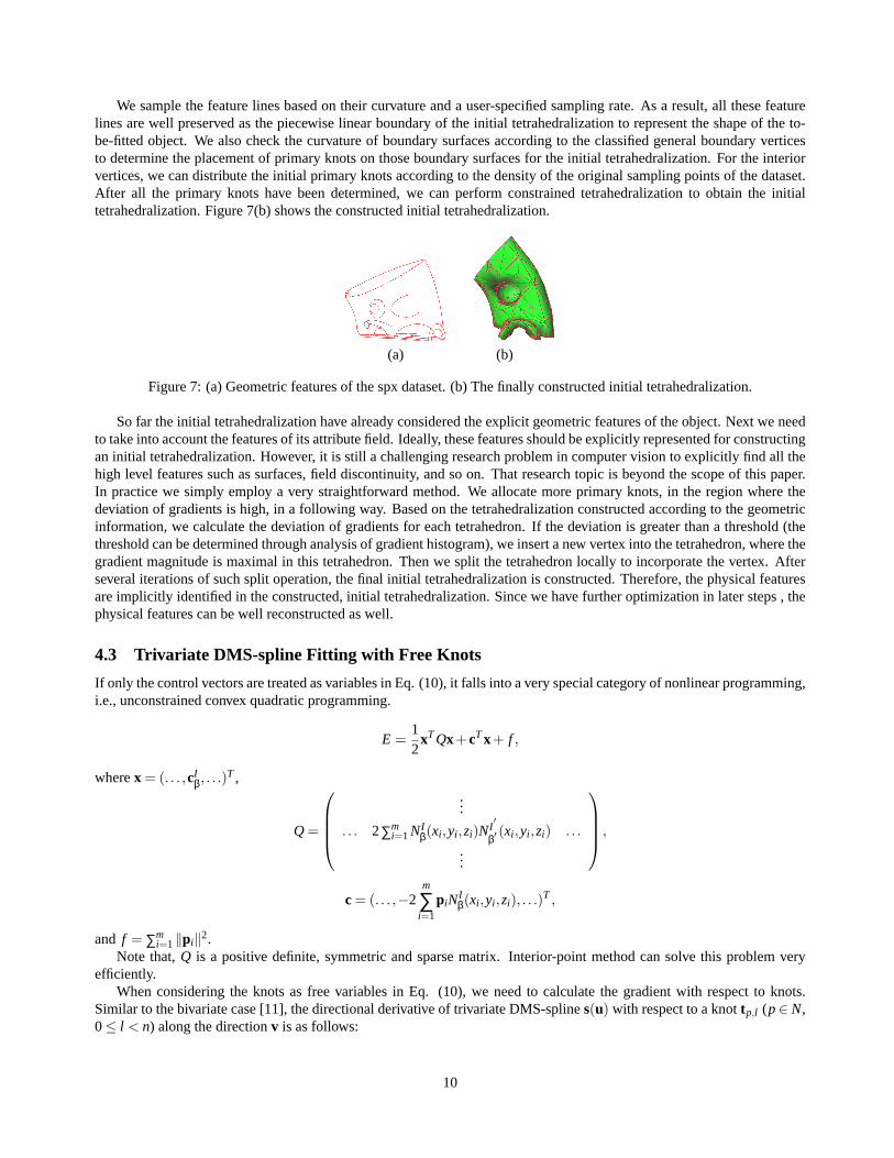
We sample the feature lines based on their curvature and a user-specified sampling rate. As a result, all these featurelines are well preserved as the piecewise linear boundary of the initial tetrahedralization to represent the shape of the to-be-fitted object. We also check the curvature of boundary surfaces according to the classified general boundary verticesto determine the placement of primary knots on those boundary surfaces for the initial tetrahedralization. For the interiorvertices, we can distribute the initial primary knots according to the density of the original sampling points of the dataset.After all the primary knots have been determined, we can perform constrained tetrahedralization to obtain the initialtetrahedralization. Figure 7(b) shows the constructed initial tetrahedralization.

(a) (b)

Figure 7: (a) Geometric features of the spx dataset. (b) The finally constructed initial tetrahedralization.

So far the initial tetrahedralization have already considered the explicit geometric features of the object. Next we needto take into account the features of its attribute field. Ideally, these features should be explicitly represented for constructingan initial tetrahedralization. However, it is still a challenging research problem in computer vision to explicitly find all thehigh level features such as surfaces, field discontinuity, and so on. That research topic is beyond the scope of this paper.In practice we simply employ a very straightforward method. We allocate more primary knots, in the region where thedeviation of gradients is high, in a following way. Based on the tetrahedralization constructed according to the geometricinformation, we calculate the deviation of gradients for each tetrahedron. If the deviation is greater than a threshold (thethreshold can be determined through analysis of gradient histogram), we insert a new vertex into the tetrahedron, where thegradient magnitude is maximal in this tetrahedron. Then we split the tetrahedron locally to incorporate the vertex. Afterseveral iterations of such split operation, the final initial tetrahedralization is constructed. Therefore, the physical featuresare implicitly identified in the constructed, initial tetrahedralization. Since we have further optimization in later steps , thephysical features can be well reconstructed as well.

4.3 Trivariate DMS-spline Fitting with Free Knots

If only the control vectors are treated as variables in Eq. (10), it falls into a very special category of nonlinear programming,i.e., unconstrained convex quadratic programming.

E =12

xTQx+cTx+ f ,

wherex = (. . . ,cIβ, . . .)

T ,

Q =

...

. . . 2∑mi=1NI

β(xi ,yi ,zi)NI′

β′(xi ,yi ,zi) . . .

...

,

c = (. . . ,−2m

∑i=1

piNIβ(xi ,yi ,zi), . . .)T ,

and f = ∑mi=1‖pi‖2.

Note that,Q is a positive definite, symmetric and sparse matrix. Interior-point method can solve this problem veryefficiently.

When considering the knots as free variables in Eq. (10), we need to calculate the gradient with respect to knots.Similar to the bivariate case [11], the directional derivative of trivariate DMS-splines(u) with respect to a knottp,l (p∈N,0≤ l < n) along the directionv is as follows:

10

Dtp,l ,vs(u) = DvG(u)+H(u,v), (11)

where

G(u) =− 1n+1 ∑

I∈Ω,i j=p∑

|β|=n+1,β j>l

cIβ−ej N(u|V I

β),

H(u,v) = ∑I∈Ω,i j=p

∑|β|=n,β j=l

µj(v|XIβ)c

IβN(u|V I

β),

andV I

β = . . . , tp,0, . . . , tp,l−1, tp,l , tp,l , tp,l+1, . . . , tp,n, . . . ,.

Note that thei j in above equation is the j-th element of 4-tupleI = (i0, . . . , i3) which represents the vertex indices of atetrahedronI .

We also need to pay special attention to the positions of knots. To describe clearly, we classify the knots into twocategories: the primary knotsts,0|s∈ N and the sub-knotsts,l |s∈ N,1≤ l ≤ n.

The primary knots must yield valid tetrahedralization inΩ and the sub-knots must satisfy Eq. (3). Especially, thesub-knots on the boundary must lie outside ofΩ. To prevent degeneracy, we also set the restriction to the minimal dis-tance between any two knots (either primary knots or sub-knots). Therefore, Eq. (10) is a typical large-scale constrainednonlinear programming problem. It is usually very time consuming for solve this kind of problem. To simplify our imple-mentation and improve the performance, we solve this problem “locally”, i.e., for each nodet i of the tetrahedralization, ifthe mean square fitting error in its adjacent neighboring tetrahedra is greater than the desired valueε, then we solve Eq.(10) by treating the knots associated tot i as free variables. Since all other knots are fixed, we can deal with a sub-problemof Eq. (10), in which onlyp j |p j is an adjacent neighbor oft i are considered.

4.4 Local Adaptive Refinement

The above volume data fitting procedure attempts to minimize the total squared distance of the volume data pointspi tothe DMS-splines. For some regions with dense points or sharp features, it is often desirable to introduce new degreesof freedom into the spline representation in order to improve the fitting quality. Therefore, we subdivide any domaintetrahedron whose fitting error is greater than the desired mean square fitting error,ε. Intuitively, local adaptive refinementis a further action for allocating tetrahedra around the feature parts. Error characterization and evaluation is an importantissue at this step. In the adaptive refinement, both geometric features and field features are considered.

For attribute data fitting, a new knot is inserted at the location, where the gradient magnitude is largest inside thetetrahedron. For solid geometry fitting, a new inserted knot should be placed on the feature line. During the optimization,the primary knots can only move along the sharp feature. This is explicitly enforced since the feature lines have beendetected. The sub-knots must lie on the feature line segment between two adjacent primary knots.

Figure 8 shows the fitting results for the spx model. A quadratic simplex spline model is used in the fitting. Figure 8(a)and (b) shows the fitting with control vectors only, while Fig. 8(c) and (d) shows the final fitting results with both controlvectors and knots. Apparently, adjusting knots can reduce the fitting error and achieve a better effect.

Figure 9(a-b) shows the fitting results for a smooth engineering part, router. Quadratic simplex spline models are usedin the fitting. Figure 9(a) is the original data set. Figure 9(b) shows the final fitting result, which is fitted using both controlvectors and knots. Figure 9(c-d) shows the fitting of two separated engineering parts. Figure 9(c) shows the original dataset. Figure 9(d) shows the final fitting result, which is fitted with both control vectors and knots.

5 Visualization Techniques

5.1 Direct Volume Rendering

Attribute distribution on a 3D solid object can be visualized in a number of ways, for example by color contours on a 2Dslice, or by a polygonal approximation to a contour surface. Direct volume rendering refers to techniques which produce aprojected image directly from the volume data, without intermediate constructs such as contour surface polygons. Amongthe direct volume rendering techniques, the ray casting approach typically casts rays from pixels in the screen into a volu-metric dataset. The quantity that is accumulated for each ray originating in each pixel is converted into color or intensityand is assigned to the pixel. It assumes datasets scatter, occlude, generate, and reflect light. Volume rendering enhances 3D

11

Figure 8: The fitting results for the spx dataset. (a)-(b) Fitting with control vectors only (front view and side view). (c)-(d)Fitting with both control vectors and knots (front view and side view).

Figure 9: Simplex spline based fitting examples. (a) The original dataset, router, in point view, where the color indicates theattribute value. (b) Fitting with both control vectors and knots. The final result is rendered using our marching tetrahedraalgorithm. (c) The original dataset, crosscube, in point view, where the color indicates the attribute value. (d) Fitting withboth control vectors and knots. The final result is rendered using the direct volume rendering algorithm.

visualization of imaged tissue by providing translucent rendering. In addition to the standard 3D image analysis tools, vol-ume rendering allows the user to interactively define thresholds for opacity, color application, and brightness. Translucentrendering of volumetric data provides more information about a spatial relationship of different structures than standard3D surface rendering. Direct volume rendering affords us the capability to isolate quickly tissue of interest, and quicklyprovides 3D spatial information for enhanced diagnostic confidence, improves surgical and treatment planning, and aidsin education. In the proposed approach, we only consider absorption nature of the dataset. That is to say that the object isvisualized by integrating the density of the trivariate simplex functions along the path of each casted ray as in [20]. The

12

intensity of light passing through translucent material decreases exponentially. Therefore,

I(a,b) = exp(−Z L

0∑I∈Ω

∑|β|=n

gIβNI

β(u(t))dt)

= exp(− ∑I∈Ω

∑|β|=n

gIβ

Z L

0NI

β(u(t))dt).

The proposed direct rendering of scalar simplex spline functions is able to incrementally update complex volumetricdata sets at interactive rates of several frames per second. Assume a control coefficientgI

β changes with∆gIβ. Then the new

intensity of the pixel will be:

Inew(a,b) = Iold(a,b)exp(−∆gIβ

Z L

0NI

β(u(t))dt). (12)

SinceNIβ(u(t))= |d(pi ,q j , r k,sl )|M(u(t)|VI

β) as shown in Eq. (5), the problem becomes how to evaluateR L

0 M(u(t)|VIβ)dt

efficiently. Grounded on the theory of simplex splines, we derive the following analytic solution to compute the integral ina recursive fashion. In the following derivation, the notations has the same meanings as in 2.1. In order to save space, weabbreviateVI

β to V. Suppose thatu(t) = xc+ tdc, wherexc anddc are constant vectors, which denote the starting point of acasted ray and the unit direction of the ray, respectively. Then whenn > 0, using the linear decomposition, we can obtain:

Z L

0M(u(t)|V)dt =

Z L

0

3

∑j=0

λ(xc + tdc)M(u(t)|V \uk j)dt

=Z L

0(

3

∑j=0

λ(xc)+ t3

∑j=0

µ(dc))M(u(t)|V \uk j)dt.

By Eq. (2) and

DdcM(u(t)|V) = d>c ∇M(u(t)|V) =dM(u(t)|V)

dt, (13)

then performing integration by parts, we can obtain,

Z L

0t

3

∑j=0

µ(dc)M(xc + tdc|V \uk j)dt

=1n

Z L

0tDdcM(xc + tdc|V)dt

= tM(xc + tdc|V)|L0−1n

Z L

0M(xc + tdc|V)dt

= −1n

Z L

0M(xc + tdc|V)dt. (14)

Replacing Eq. (14) in Eq. (13), we can obtain the following equation:

Z L

0M(xc + tdc|V)dt =

nn+1

3

∑j=0

λ(xc)Z L

0M(u(t)|V \uk j)dt. (15)

Whenn = 0, Z L

0M(xc + tdc|V)dt =

LVol(V)

.

With the above equation, we can efficiently evaluate the integral of densities along a casted line. Besides the X-rayvolume rendering, we can also perform general ray casting. Since the solid object is represented by a single trivariateDMS-spline, our ray casting avoids resampling and interpolation problems.

13

5.2 Marching Tetrahedra Isosurfacing

Since the resulting heterogeneous solid object consists of tetrahedra, it is easy to perform marching tetrahedra isosurfacingto extract an isosurface of its associated field. It is important to note that, based on the geometry of the primary knots,the samples may be spaced at non-unit intervals or distributed very irregularly. Our approach does not require resamplingonto a regular voxel raster, which would introduce error. Furthermore, along tetrahedron edges, the process of isosurfaceextraction employs the original trivariate DMS-spline interpolation, which has the potential to avoid introducing samplingartifacts. Since traditional voxel-based sculpting systems employ trilinear interpolation, they exhibit aliasing when thevoxel grid is scaled or deformed. Aliasing must then be eliminated by filtering most or all of the voxel grid. We avoid thisproblem by using what is essentially a higher-orderCn−1 trivariate spline. If the material distribution of an object modeledby our approach is originally smooth, it will remain smooth even if the control lattice is arbitrarily scaled or even deformed,as long as there is no self-intersections occurred. If it contains discontinuity region, these features will be preserved as well.

A key aspect of isosurface extraction is normal vector computation. With our polynomial-based approach, it canbe determined analytically. Furthermore, the local evaluation can lead to multiresolution isosurface extraction. When atetrahedron of the object is determined cross the isosurface of its associated field, and its size is larger than a specifiedthreshold, we can evaluate the trivariate DMS-spline and upsample it locally to increase the resolution and then performisosurfacing on those smaller cells.

6 Implementation and Discussion

We have implemented a prototype system on a PC with 3.0 GHz P4 CPU and 2GB of RAM. The system is written in C++and OpenGL. Table 1 shows the statistics of the performance of our fitting algorithm on several datasets, where the fittingerror is the mean square error.

Model data pts domain tetra control pts knots geometric fitting error field fitting error

spx 15832 1914 3335 992 8.21121×10−7 7.78170×10−4

cubecross 24128 2245 3294 858 1.25994×10−6 1.97281×10−4

router 34744 2812 4239 1236 1.13400×10−6 1.52832×10−4

Table 1: Statistics of Data fitting.

As one can see, we couple geometric and attribute representation together in order to provide a unified paradigm toexplicitly model geometry, topology, and its associated attribute properties. However, one weakness of this representationis that if the geometric features and attribute field features are not conforming to each other, we have to select the higherresolution to model both, even though it might not necessary for one of them to have such a high resolution. A potentialsolution for this case is to decouple geometric and attribute representations. Thus, it offers more flexibility to constructdifferent resolution of tetrahedralization of a domain to fit the geometry and attribute distribution, respectively. But specialcare must be taken in aligning the boundaries of two domains exactly the same, or else some locations of the geometricobject may not have attribute properties, or attribute properties are assigned to the locations outside the geometric object.When using the decoupling scheme, it is possible to model any number of attribute properties over the geometric object.Complicated geometries with simple attributes, and vice versa, may be represented at the resolution that best suits them.The gain may be a large savings in storage and execution time.

Furthermore, noise is an important variable in any visualization involving measured data. Simplex splines generallyprovide a robust representation for a signal containing moderate noise. Compared with polygons, or higher dimensionalanalogues such as voxels, simplex splines generally represent a smooth function with fewer points. However, with ourknots manipulation technique they can represent higher frequency features as well.

7 Conclusion

In this paper we have articulated a new integral approach for representing, modeling, reconstructing, and visualizing mul-tidimensional, physical attributes across any volumetric objects. In particular, we employ a trivariate simplex spline modelthat is defined over a tetrahedral decomposition of any 3D domain. The modeled volume can be of complicated geometry

14

and topology. The trivariate simplex spline model ideally serves the pressing needs of modeling and visualization of inho-mogeneous objects in engineering design. The model can offer a compact continuous representation. More importantly,it integrates geometry and attribute properties over domains complex topology, by modeling a complicated heterogeneousobject with a single trivariate simplex spline without any additional operations of trimming or patching. All of the aboveattractive characteristics result from many appealing properties of trivariate simplex splines such as piecewise polynomialsof low degree, high-order continuity, and sharp feature modeling through different knot placements. In addition, we havedeveloped a feature-sensitive fitting algorithm that can reconstruct a more compact trivariate simplex spline from a struc-tured or unstructured volume. It reconstructs the geometry and the associated material attributes simultaneously, satisfyingvarious continuity requirements set by the user. Such flexibility allows us to model continuous or discontinuous materialdistribution with ease.

Our new representation can also facilitate multiresolution, local adaptive subdivision, free-form deformation, bothisosurface and volume rendering, as well as other modeling and visualization functionalities. This is mainly because manyof its nice analytical properties and associated computational tools. Based on our extensive experiments on using thetrivariate simplex spline, we believe that our new paradigm can significantly advance the current state of the knowledgein modeling and visualizing heterogeneous models of physical objects and their material properties in engineering design.In the near future we plan to pursue other application directions including material editing and reconstruction, dynamicsimulation and analysis of multiresolution, heterogeneous objects, etc.

References

[1] Raviv, A., and Elber, G., 1999, “Three Dimensioinal Freeform Sculpting Via Zero Sets of Scalar Trivariate Functions,”Proceedings of the 5th ACM Symposium on Solid Modeling and Applications, pp. 246–257.

[2] Hua, J., and Qin, H., 2004, “Haptics-based Dynamic Implicit Solid Modeling,”IEEE Trans. on Visualization andComputer Graphics, 10(5), pp. 574–586.

[3] Schmitt, B., Pasko, A., and Schlick C., 2001, “Constructive Modeling of FRep Solids Using Spline Volumes,”Proceedings of the 6th ACM symposium on Solid modeling and applications, pp. 321–322.

[4] Martin, W., and Cohen, E., 2001, “Representation and Extraction of Volumetric Attributes Using Trivariate Splines:A Mathematical Framework,”Proceedings of the 7th ACM Symposium on Solid Modeling and Applications, pp.234–240.

[5] Dahmen, W., Micchelli, C., and Seidel, H., 1992, “Blossoming Begets B-spline Bases Built Better by B-patches,”Mathematics of Computation, 59(199), pp. 97–115.

[6] de Boor, C., 1976, “Splines as Linear Combinations of B-splines,”Approximation Theory II, Academic Press, NewYork, pp. 1–47.

[7] Greiner, G., and Seidel, H., 1994, “Modeling with Triangular B-splines,”IEEE Computer Graphics and Applications,14(2), pp. 56–60.

[8] Pfeifle, R., and Seidel, H., 1994, “Faster Evaluation of Quadratic Bivariate DMS Spline Surfaces,”Proceedings ofGraphics Interface, pp. 182–189.

[9] Pfeifle, R., and Seidel, H., 1995, “Fitting Triangular B-splines to Functional Scattered Data,”Proceedings of GraphicsInterface, pp. 80–88.

[10] Qin, H., and Terzopoulos, D., 1997, “Triangular NURBS and Their Dynamic Generalizations,” Computer-AidedGeometric Design,14(4), pp. 325–347.

[11] He, Y., and Qin, H., 2004, “Surface Reconstruction with Triangular B-splines,”Proceedings of Geometric Modelingand Processing, pp. 279–291.

[12] Seidel, H., and Vermeulen, A., 1994, “Simplex Splines Support Surprisingly Strong Symmetric Structures andSubdivision,”Curves and Surfaces II, AK Peters, pp. 443–455.

15

[13] Joe, B., 1991, “Construction of Three-Dimensional Triangulations Using Local Transformations,” Computer AidedGeometric Design,8, pp. 123–142.

[14] Edelsbrunner, H., and Shah, N., 1992, “Incremental Topological Flipping Works for Regular Triangulations,”Pro-ceedings of ACM Symposium on Computational Geometry, pp. 43–52.

[15] Shewchuk, J., 1997, “Delaunay Refinement Mesh Generation,” Ph.D. thesis, School of Computer Science, CarnegieMellon University.

[16] Biswas, A., Shapiro, V., and Tsukanov, I., 2004, “Heterogeneous Material Modeling with Distance Fields,” ComputerAided Geometric Design,21(3), pp. 215–242.

[17] Zhou, Y., Chen, B., and Kaufman, A., 1997, “Multiresolution Tetrahedral Framework for Visualizing Regular VolumeData,” Proceedings of IEEE Visualization Conference, pp. 135–142.

[18] Liu, A., and Joe, B., 1994, “Relationship between Tetrahedron Shape Measures,” BIT,34(2), pp. 268–287.

[19] Hong, W., and Kaufman, A., 2003, “Feature Preserved Volume Simplification,”Proceedings of the 8th ACM Sympo-sium on Solid Modeling and Applications, pp. 328–333.

[20] Raviv, A., and Elber, G., 2001, “Interactive Direct Rendering of Trivariate B-spline Scalar Functions,”IEEE Trans.on Visualization and Computer Graphics, 7(2), pp. 109–119.

16