Embed Size (px)
Citation preview
Trond Martin Augustson
VISION BASED IN-SITU CALIBRATION OF ROBOTS WITH APPLICATION IN SUBSEA INTERVENTIONS
M.Sc. Thesis
Thesis presented to obtain the M.Sc. title at the Mechanical Engineering Department at PUC-Rio.
Advisor: Marco Antonio Meggiolaro
Rio de Janeiro September 2007
Trond Martin Augustson
CALIBRAGEM VISUAL IN SITU DE MANIPULADORES ROBÓTICOS COM APLICAÇÃO EM INTERVENÇÕES
SUBMARINAS
Dissertação apresentada como requisito parcial para obtenção do grau de Mestre pelo Programa de Pós-Graduação em Engenharia Mecânica do Departamento de Engenharia Mecânica do Centro Técnico Científico da PUC-Rio. Aprovada pela Comissão Examinadora abaixo assinada.
Prof. Marco Antonio Meggiolaro Orientador
Pontifícia Universidade Católica do Rio de Janeiro
Prof. Mauro Speranza Neto Pontifícia Universidade Católica do Rio de Janeiro
Prof. Raul Queiroz Feitosa
Pontifícia Universidade Católica do Rio de Janeiro
Prof. Fernando Cesar Lizarralde Universidade Federal do Rio de Janeiro
Prof. José Eugenio Leal Coordenador Setorial do Centro
Técnico Científico – PUC-Rio
Rio de Janeiro, 3 de setembro de 2007
All rights reserved. Any reproduction of this work without authorization from the university, the author and the advisor is prohibited.
Trond Martin Augustson Graduated in applied physics at The University of Bergen in 1998. He has worked with seismic surveying until entering the master program at PUC-Rio in 2005.
Ficha Catalográfica
CDD: 621
Augustson, Trond Martin Vision based in-situ calibration of robots with
application in subsea interventions / Trond Martin Augustson ; orientador: Marco Antonio Meggiolaro. – 2007.
143 f. : il.(col.) ; 30 cm Dissertação (Mestrado em Engenharia
Mecânica)–Pontifícia Universidade Católica do Rio de Janeiro, Rio de Janeiro, 2007.
Inclui bibliografia 1. Engenharia mecânica – Teses. 2. Robotics.
3. Calibration. 4. Computer vision. 5. SIFT. 6. Patern recognition. 7. Automation. 8. Stereopsis. I. Meggiolaro, Marco Antonio. II. Pontifícia Universidade Católica do Rio de Janeiro. Departamento de Engenharia Mecânica. III. Título.

Thanks to
• My advisor Marco Antonio Meggiolaro, for help and support;
• Professor Raul Feitosa, for the contribution on computer vision;
• PUC-Rio for the opportunity and the great academic environment
that constitute the basis of this work;
• CENPES/PETROBRAS for the support, including the submarine
camera and information on the TA-40 manipulator;
• My family, however distant, supporting me during my work.
Abstract Augustson, Trond Martin; Meggiolaro, Marco Antonio (Orientador). VISION BASED IN-SITU CALIBRATION OF ROBOTS WITH APPLICATION IN SUBSEA INTERVENTIONS. Rio de Janeiro 2007, 143p. M.Sc. Dissertation –Mechanical Engineering Department, Pontifícia Universidade Católica do Rio de Janeiro.
The majority of today’s industrial robots are programmed to follow a predefined trajectory. This is sufficient when the robot is working in a fixed environment where all objects of interest are situated in a predetermined position relative to the robot base. However, if the robot’s position is altered all the trajectories have to be reprogrammed for the robot to be able to perform its tasks. Another option is teleoperation, where a human operator conducts all the movements during the operation in master-slave architecture. Since any positioning errors can be visually compensated by the human operator, this configuration does not demand that the robot has a high absolute accuracy. However, the drawback is the low speed and low accuracy of the human operator scheme. The manipulator considered in this thesis is attached to a ROV (Remote Operating Vehicle) and is brought to its working environment by the ROV operator. Every time the robot is repositioned, it needs to estimate its position and orientation relative to the work environment. The ROV operates at great depths and there are few sensors which can operate at extreme depths. This is the incentive for the use of computer vision to estimate the relative position of the manipulator. Through cameras the differences between the actual and desired position of the manipulators is estimated. This information is sent to controllers to correct the pre-programmed trajectories. The manipulator movement commands are programmed off-line by a CAD system, without need even to turn on the robot, allowing for greatest speed on its validation, as well as problem solving. This work includes camera calibration and calibration of the structure of the manipulator. The increased accuracies achieved by these steps are merged to achieve in-situ calibration of the manipulator base.
Key Words Robotics; Calibration; Computer vision; SIFT; Pattern recognition;
Automation; Stereopsis
Resumo Augustson, Trond Martin; Meggiolaro, Marco Antonio (Advisor). CALIBRAGEM VISUAL IN SITU DE MANIPULADORES ROBÓTICOS COM APLICAÇÃO EM INTERVENÇÕES SUBMARINAS. Rio de Janeiro 2007, 143p. Dissertação de Mestrado – Departamento de Engenharia Mecânica, Pontifícia Universidade Católica do Rio de Janeiro.
A maioria dos robôs industriais da atualidade são programados para seguir uma trajetória pré-definida. Isto é suficiente quando o robô está trabalhando em um ambiente imutável onde todos os objetos estão em uma posição conhecida em relação à base do manipulador. No entanto, se a posição da base do robô é alterada, todas as trajetórias precisam ser reprogramadas para que ele seja capaz de cumprir suas tarefas. Outra opção é a teleoperação, onde um operador humano conduz todos os movimento durante a operação em uma arquitetura mestre-escravo. Uma vez que qualquer erro de posicionamento pode ser visualmente compensado pelo operador humano, essa configuração não requer que o robô possua alta precisão absoluta. No entanto, a desvantagem deste enfoque é a baixa velocidade e precisão se comparado com um sistema totalmente automatizado. O manipulador considerado nesta dissertação está fixo em um ROV (Remote Operating Vehicle) e é trazido até seu ambiente de trabalho por um teleoperador. A cada vez que a base do manipulador é reposicionada, este precisa estimar sua posição e orientação relativa ao ambiente de trabalho. O ROV opera em grandes profundidades, e há poucos sensores que podem operar nestas condições adversas. Isto incentiva o uso de visão computacional para estimar a posição relativa do manipulador. A diferença entre a posição real e a desejada é estimada através do uso de câmeras submarinas. A informação é enviada aos controladores para corrigir as trajetórias pré-programadas. Os comandos de movimento do manipulador podem então ser programados off-line por um sistema de CAD, sem a necessidade de ligar o robô, permitindo rapidez na validação das trajetórias. Esse trabalho inclui a calibragem tanto da câmera quanto da estrutura do manipulador. As melhores precisões absolutas obtidas por essas metodologias são combinadas para obter calibração in-situ da base do manipulador.
Palavras-Chave Robótica; Calibragem; Visão computacional; SIFT; Reconhecimento de
padrões; Automação; Visão estéreo
Summary
1 Introduction 20
1.1. Motivation 20
1.2. Work objectives 20
1.3. Work description 21
1.4. Organization of the Thesis 24
2 Kinematic Modeling for Calibration of Manipulators 26
2.1. Introduction 26
2.2. Basic Concepts of Kinematics 28
2.3. The Denavit-Hartenberg Convention 29
2.4. Classic Manipulator Calibration 32
2.5. Elimination of Redundant Errors 36
2.6. Physical Interpretation of the Redundant Errors 38
2.7. Partial Measurement of End-Effector Pose 39
2.8. Inverse Kinematics 40
2.8.1. Solvability 40
2.9. Experimental Procedures 41
3 Computer Vision 47
3.1. Introduction 47
3.2. Mathematic Camera Models 48
3.2.1. The Pinhole Model 48
3.2.2. Intrinsic Parameters 49
3.2.3. Extrinsic Parameters 51
3.3. Camera Calibration 52
3.3.1. Radial Distortion 56
3.3.2. Sophisticated calibration 58
3.3.3. Coordinate extraction 61
3.3.4. Nonmaximum Suppression 61
3.3.5. K-means Line Fitting 63
3.4. Feature Matching 64
3.4.1. Detection of Interest Points 65
3.4.2. Elimination of Edge Responses 66
3.4.3. Accurate keypoint localization 67
3.4.4. Assigning Orientation 68
3.4.5. The Key-Point Descriptor 69
3.4.6. Invariance to orientation and illumination 70
3.4.7. Keypoint matching 71
3.5. Triangulation 73
3.6. Stereo Vision 76
3.7. Manipulator Base Calibration 78
3.7.1. Quaternion Algebra 79
3.7.2. Estimation of the Rotation Matrix Using Quaternions 80
3.8. Elimination of Keypoint Matches using RANSAC 83
3.9. Triangulation Using the Kinematics of the Manipulator 85
4 Application to the TA-40 Manipulator 90
4.1. Introduction 90
4.2. Description of the Manipulator 90
4.3. Kinematics of the TA-40 91
4.3.1. Joints 1 and 2 93
4.3.2. Joints 2 and 3 93
4.3.3. Joints 3 and 4 93
4.3.4. Joints 4 and 5 93
4.3.5. Joints 5 and 6 94
4.3.6. Joint 6 94
4.3.7. Denavit-Hartenberg Parameters 94
4.4. Calibration of the TA-40 95
4.5. Inverse Kinematics 96
4.6. Orientation Error of the Manipulator 101
5 Results 108
5.1. Introduction 108
5.2. Laboratory Experiments 108
5.2.1. Camera Calibration 110
5.2.2. Experiments with the X-Y Table 113
5.3. Calibration of an Underwater Camera 123
5.4. Position Estimation using the Underwater Camera 125
5.5. Camera Calibration performed Underwater 132
6 Conclusions and Suggestions 134
6.1. Conclusions 134
6.2. Suggestions for future work 135
7 References 136
Appendix A 139
List of figures
Figure 1 - Repeatability and absolute accuracy........................................ 21
Figure 2 - Coordinate systems of the manipulator .................................... 27
Figure 3 - Denavit-Hartenberg parameters [5] .......................................... 30
Figure 4 -Translation and rotation with effects of errors in the i-th
link [6] ................................................................................................. 32
Figure 5 - Generalized errors for the i-th link. εp,i, εs,i, εr,i represent
the rotation around the x,y and z-axes respectively. [6] .................... 33
Figure 6 – Error compensation block diagram [6] ..................................... 35
Figure 7 – Combination of translational linear errors [6]........................... 38
Figure 8 – Simplified combination of error [6] ........................................... 39
Figure 9 – Finding the rotation axis of joint 2 (Z1), side view.................... 42
Figure 10 – Finding the rotation axis of joint 1 (Z0), upper view ............... 42
Figure 11 - The trajectory of the probe forms a plane that is found
by a least square approximation........................................................ 43
Figure 12 - Angles between the laser tracker reference frame and
the normal plane [12] ......................................................................... 44
Figure 13 - Schematic representation of the pinhole model ..................... 48
Figure 14 – Geometry of the pinhole model [14]....................................... 49
Figure 15 - CCD layout. (a) shows an ideal square, (b) shows that
the scale in x and y direction can differ, (c) shows that the axes
might not be perpendicular [14]. ........................................................ 49
Figure 16 - The modified pinhole model. [14] ........................................... 50
Figure 17 - The image center is not always in the middle of the
sensor since the lens normal does not intersect with the middle
of the sensor panel............................................................................. 50
Figure 18 – Transformation of world coordinates to camera
coordinates. [14]................................................................................. 52
Figure 19 – Calibration rig......................................................................... 53
Figure 20 - Transformation from world coordinates to picture
coordinates. [14]................................................................................. 53
Figure 21 - Types of radial distortion......................................................... 56
Figure 22 – Principle of barrel distortion. The black coordinates
represent the image coordinates for a camera without
distortion. The violet coordinates show the distorted image
coordinates......................................................................................... 57
Figure 23 – The 4 directions used in nonmaximum suppression ............. 62
Figure 24 – Output of the nonmaximum suppression algorithm............... 63
Figure 25 – Maxima and minima in the Difference-of-Gauss are
compared to its 26 neighbors [3]........................................................ 66
Figure 26 – Histogram of key-point orientation [3]. ................................... 69
Figure 27 - Keypoint calculation process. Each 4x4 element of
gradients (left) is referred to as a bin. For each bin a histogram
of 8 directions is calculated (right) [3] ................................................ 70
Figure 28 – Distribution of relative keypoint orientation............................ 72
Figure 29 – Triangulation .......................................................................... 73
Figure 30 – Stereo Triangulation............................................................... 76
Figure 31 –Initial procedure to estimate the position of the
reference camera relative to the keypoints. Creating a set of
3D coordinates, 1 p . ........................................................................... 86
Figure 32 – Finding a second set of corresponding coordinates, 2 p
. .......................................................................................................... 88
Figure 33 – TA40 and the miniature robot used as master ...................... 91
Figure 34 – TA-40 and coordinate systems [1] ......................................... 92
The frame center O4 of joint 5 is located 747mm along the z4 axis
from O4, giving d4=747. Since the frame centers position along
the common normal is zero, a4=0. The z4 axis is rotated -90º
relative to z3, giving α4=-90º. .............................................................. 93
Figure 35 - A 2D interpretation of the frames O2,O3 and O4. Frame
O5 coincides with frame O4 [24]. ........................................................ 97
Figure 36 - Position error of end-effector after calibration ...................... 104
Figure 37 - Rotation error at the end effector after calibration................ 105
Figure 38 - Position error of link 5 after calibration ................................. 106
Figure 39 - Rotation error of link 5 after calibration ................................ 107
Figure 40 – x-y table in the Robotics laboratory at PUC......................... 109
Figure 41 – Calibration rig....................................................................... 109
Figure 42 – Edges of the calibration rig. The estimated corners are
marked in red. .................................................................................. 110
Figure 43 – Figure showing the edges of the image in white. The
image to the left shows the initial k-mean line parameters. The
image on the right shows the improved estimate after only
three iterations. The estimated coordinate of the corner is
marked in red. The yellow and green lines show the estimated
lines. ................................................................................................. 111
Figure 44 – Relative movement between extracted coordinates and
the projected coordinates................................................................. 113
Figure 45 - The robot used as reference object in the experiment......... 114
Figure 46 – Coordinate system of the x-y table ...................................... 114
Figure 47 – Method to estimate the set of coordinates, 2 p . The
reference image is marked in yellow. The position of one of the
two cameras is to be estimated relative to the reference image. .... 118
Figure 48 – Triangulation to estimate the coordinate set 1 p relative
to the origin. The reference image is marked in yellow. The
images closest to the reference image and the two cameras
used to estimate the coordinate set 2 p were not used. .................. 118
Figure 49 – RMS position error as a function of intraocular distance
using RANSAC and quaternion rotation estimation......................... 120
Figure 50 – Graph showing the average RMS position error as a
function of the intraocular distance after the samples with the
worst error ratio had been removed................................................. 121
Figure 51 - RMS position error as a function of intraocular distance
using RANSAC with LMS rotation estimate..................................... 122
Figure 52 - RMS position error as a function of intraocular distance
using RANSAC with LMS rotation estimate and eliminating the
coordinates with a high error ratio. .................................................. 123
Figure 53 –The corrected image coordinates relative to their
respective extracted image coordinates .......................................... 125
Figure 54 – Attachment support for the underwater camera. ................. 126
Figure 55 – Position accuracy as a function of the intraocular
distance using all 72 coordinates and quaternion rotation
estimation......................................................................................... 128
Figure 56 - Position accuracy as a function of the intraocular
distance after the coordinates with a large error ratio had been
eliminated......................................................................................... 129
Figure 57 - Position error as a function of intraocular distance with
the underwater camera using all 72 coordinates and LMS
rotation estimation............................................................................ 130
Figure 58 - Position accuracy as a function of the intraocular
distance after the coordinates with a large error ratio had been
eliminated......................................................................................... 131
Figure 59 – Underwater calibration. The green points are the
corrected image coordinates and the red lines show their
respective image coordinates .......................................................... 133
Figure A.1 – Coordinate systems of the TA-40....................................... 139
List of Tables
Table 1 – Denavit-Hartenberg parameters ............................................... 94
Table 2 – Errors from simulation ............................................................. 103
Table 3 – Camera calibration parameters............................................... 112
Table 4 – Position parameters for the experiment.................................. 115
Table 5 – Position error as a function of intraocular distance using
RANSAC .......................................................................................... 119
Table 6 – Position error as a function of intraocular distance using
RANSAC and error ratio elimination. ............................................... 120
Table 7 - Position error as a function of intraocular distance using
RANSAC together with the least mean square estimated
rotation matrix. ................................................................................. 121
Table 8 - Position error as a function of intraocular distance using
RANSAC together with the least mean square estimated
rotation matrix and eliminating the coordinates with error ratio....... 122
Table 9 –Calibration parameters for the underwater camera in air,
where su is the aspect ratio, f is the focal length, k1 and k2 are
the radial distortion coefficients, T1 and T2 are the tangential
distortion coefficients and (uo,vo ) denotes coordinates of the
image center. ................................................................................... 124
Table 10 – Position parameters for the experiment with the
underwater camera. ......................................................................... 127
Table 11 – Position error as a function of intraocular distance using
the underwater camera, all 72 coordinates, and quaternion
rotation estimation............................................................................ 128
Table 12 - Position accuracy as a function of the intraocular
distance after the coordinates with a large error ratio had been
eliminated......................................................................................... 129
Table 13 – Position error as a function of intraocular distance using
the underwater camera using all 72 coordinates and LMS
rotation estimation............................................................................ 130
Table 14 - Position accuracy as a function of the intraocular
distance after the coordinates with a large error ratio had been
eliminated......................................................................................... 131
Table 15 – Calibration parameters for the underwater camera in air,
where su is the aspect ratio, f is the focal length, k1 and k2 are
the radial distortion coefficients, T1 and T2 are the tangential
distortion coefficients and (uo,vo ) denotes coordinates of the
image center. ................................................................................... 132
List of Variables
Aq – Observation matrix used in quaternion rotation estimation
Ca – Observation matrix for plane estimation `aC – Observation matrix for arc coordinates projected onto the estimated plane
Ct – Observation matrix for translated coordinates used to estimate circle
parameters
Ge – Non singular Identification matrix where the redundant errors have been
eliminated. 0
nT - homogeneous matrix 4x4 that describes the orientation and position of the
manipulator end-effector relative to its base as a function of the angles of the links
θn and the generalized errors ε.
ai – Denavit-Hartenberg parameter: length of the common normal between two
adjacent links
a – quaternion vector
0 1 2 3, , ,a a a a - quaternion vector components of a.
pa - parameter for an estimated 3D plane
la - line parameter used to estimate a line through least square approximation
b - quaternion vector
0 1 2 3, , ,b b b b - quaternion vector components
bt – parameter used to estimate a circle from translated arc parameters
bq – vector used in quaternion rotation estimation
lb - line parameter used to estimate a line through least square approximation
pb - parameter for an estimated 3D plane
lc - line parameter used to estimate a line through least square approximation
pc - parameter for an estimated 3D plane
cr – estimated radius of projected circle
dmnop – variable used in deduction of triangulation principles
pd - parameter for an estimated 3D plane
di – Denavit-Hartenberg parameter: distance between the origin Oi-1 and Hi
dint – Intraocular distance between two camera centers
dn – distance limit that denotes the maximum allowed distance from the nearest
corresponding coordinate
,r id – a coordinates’ distance from the cluster center ~
1R p
0e - matrix containing the edge angle of an image
i – complex quaternion unit vector
j – complex quaternion unit vector
k – complex quaternion unit vector
k – quaternion rotation axis given by k = [i j k]
pn - normal vector for estimated plane
p - coordinate in the normalized in the normalized image plane 1 p - 3D coordinate set relative to the origin 2 p - 3D coordinate set corresponding to 1 p with a different reference frame 1
R p – translated coordinate set, used in RANSAC algorithm
~1
R p – estimated center of the translated coordinate set 1R p
q – quaternion vector
0 1 2 3, , ,q q q q - quaternion vector components of q
,e ir – error ratio of a coordinate, denoting its position error relative to its distance
from the center of the cluster.
limr – error ratio limit, denoting the accepted error ratio ,e ir
rr – estimated radius of projected circle
u - normalized x-coordinate of an image relative to the image center
v - normalized y-coordinate of an image relative to the image center
u∨
- image x-coordinate corrected for radial distortion
v∨
- image y-coordinate corrected for radial distortion
ut – output vector from least square estimate of a circle
pv - least square vector estimated by a lest square of Ca
`ax - x coordinate of an arc projected onto plane
xi – coordinate of joint i in the Denavit-Hartenberg notation
xq – substitution parameter used in quaternion deduction
xr – estimated x-coordinate of circle center
xt – translated x-coordinate used to estimate circle parameters
xtri – coordinate defining a point used in triangulation
ya – y-coordinate of an arc projected onto plane
yq – substitution parameter used in quaternion deduction
yr – estimated y-coordinate of circle center
yt – translated x-coordinate used to estimate circle parameters
ytri –coordinate defining a point used in triangulation
yi – coordinate of joint i in the Denavit-Hartenberg notation
zi – coordinate of joint i in the Denavit-Hartenberg notation
ztri –coordinate defining a point used in triangulation
Ca – observation matrix of arc coordinates relative to the laser tracker 'aC – matrix containing the projected coordinates of Ca
G – matrix containing the edge magnitude of an image
Gx – matrix containing the edge magnitude in x direction of an image
Gy– matrix containing the edge magnitude in y direction of an image
Sx – Sobel filter mask for detecting edges in x direction
Sy – Sobel filter mask for detecting edges in y direction
Lo – observation matrix for camera calibration
M – projection matrix of the pin hole camera
Mv – projection matrix in vector form
cO – camera reference frame wO – world reference frame cP – coordinate relative to the camera reference frame wP – coordinate relative to the world reference frame
Q – skew matrix used to calculate vector product
R – rotation matrix defining the relative rotation between two views
∆X- difference between desired position of the manipulator end-effector and the
actual position.
tX∆ -matrix containing differences between desired position of the manipulator
end-effector and the true measured position.
Jt - The matrix 6m x 6(n+1) formed by m Identification Jacobians, called the
Total Identification matrix
α – magnification factor in x direction for the pin hole model [pixels]
β – magnification factor in y direction for the pin hole model [pixels]
αi – Denavit-Hartenberg parameter: the angle between the joint axes in the right
hand sense.
ε - vector containing the estimated generalized errors
ε· - vector where the redundant errors are incorporated in the non redundant errors
εx,i - Generalized error of joint i along x-axis
εy,i - Generalized error of joint i along y-axis
εz,i - Generalized error of joint i along z-axis
εp,i - Generalized rotational error of joint i around x-axis
εs,i - Generalized rotational error of joint i around y-axis
εr,i - Generalized rotational error of joint i around z-axis
1γ , 2γ - multiplication factors that determines at what coordinate the closest
mutual point is found for two lines in 3D
θi – Denavit-Hartenberg parameter: the angle between the xi-1 axis and the
common normal HiOi measured along the z-azis
,p xθ – estimated angle around the x-axis, between the normal plane and the
reference frame.
,p yθ – estimated angle around the y-axis, between the normal plane and the
reference frame.
θq – quaternion rotation angle
0xθ - camera bias angle around x-axis
0yθ - camera bias angle around y-axis
0zθ - camera bias angle around z-axis
ζ – substitution variable used in estimation of quaternion rotation angle
ρ – substitution variable used in estimation of quaternion rotation angle
1 Introduction
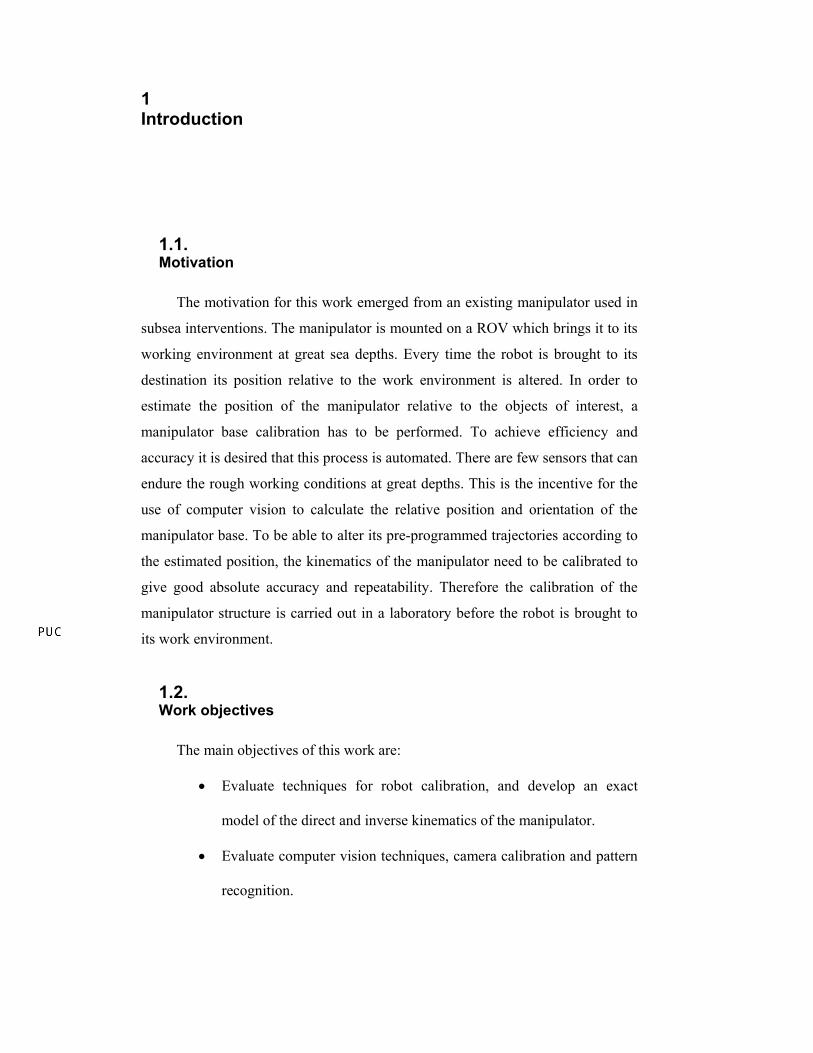
1.1. Motivation
The motivation for this work emerged from an existing manipulator used in
subsea interventions. The manipulator is mounted on a ROV which brings it to its
working environment at great sea depths. Every time the robot is brought to its
destination its position relative to the work environment is altered. In order to
estimate the position of the manipulator relative to the objects of interest, a
manipulator base calibration has to be performed. To achieve efficiency and
accuracy it is desired that this process is automated. There are few sensors that can
endure the rough working conditions at great depths. This is the incentive for the
use of computer vision to calculate the relative position and orientation of the
manipulator base. To be able to alter its pre-programmed trajectories according to
the estimated position, the kinematics of the manipulator need to be calibrated to
give good absolute accuracy and repeatability. Therefore the calibration of the
manipulator structure is carried out in a laboratory before the robot is brought to
its work environment.
1.2. Work objectives
The main objectives of this work are:
• Evaluate techniques for robot calibration, and develop an exact
model of the direct and inverse kinematics of the manipulator.
• Evaluate computer vision techniques, camera calibration and pattern
recognition.
21
• Develop methods to estimate the relative position of the manipulator
end-effector through recognition of features extracted from images.
• Simulate the techniques used on the robot to test the viability of the
procedures through experiments.
1.3. Work description
The goal of this thesis is to develop visual calibration methods to allow a
robotic manipulator to localize itself with respect to its environment. The
procedures are applied to the robot TA-40 [23] with 6 rotational joints and 6
degrees of freedom. This manipulator is used in underwater interventions and will
be attached to a ROV which will transport it to its work environment. In order to
execute pre-programmed trajectories from different locations, it is necessary to
establish an exact model of the kinematics of the manipulator. The first step of the
procedure involves calibration of the manipulator structure. It is necessary that the
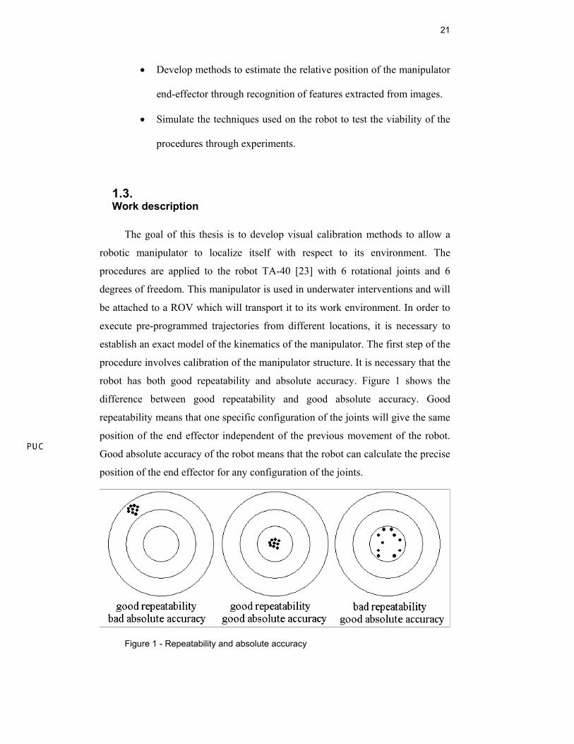
robot has both good repeatability and absolute accuracy. Figure 1 shows the
difference between good repeatability and good absolute accuracy. Good
repeatability means that one specific configuration of the joints will give the same
position of the end effector independent of the previous movement of the robot.
Good absolute accuracy of the robot means that the robot can calculate the precise
position of the end effector for any configuration of the joints.
Figure 1 - Repeatability and absolute accuracy
22
Calibration of robots is a process where the accuracy is improved by
modifying the control software of the robot to compensate the errors in the
nominal measurements of the physical structure.
The calibration process can be divided into 4 steps:
1) Elaborate a mathematical model to represent the kinematic
movement of the manipulator.
2) Measure the position of the end-effector of the manipulator.
3) Estimate the relation between the joints angles and the position of
the end-effector.
4) Compensate the deviations between the ideal estimate of the end-
effector positions and the measured positions by updating the control
software.
The steps involving selection of mathematical model, identification and
compensation of errors are studied in [1] and [2].
To improve the geometric model of a robot by calibration, the proposed
method uses a certain number of measurements of the 3D position of the robot
end-effector. Together with the measured angles of all the joints, the errors of all
the joints are estimated.
Due to the high versatility of the ROV, the robot will be working in many
different environments. Every time the robot is introduced to its work
environment, the relative position of the robot base has to be estimated in order to
be able to execute preprogrammed tasks or simply give a feedback to the operator
of the robot’s position by means of virtual reality.
This thesis follows modern tendencies of automation that has an increasing
emphasis on robots guided by sensors, automating totally or partially many of the
tasks to be executed. Cameras linked to the controller detect the actual position of
the robot automatically. The control software will automatically be updated so
that the pre-programmed trajectories can be executed automatically. The
trajectories will be programmed with a CAD system. This means that they can be
estimated in a graphic environment without using the robot, allowing a greater
velocity in the validation of trajectories.
23
To make these techniques possible, it is necessary that the robot has both
good repeatability and accuracy. This will be achieved by means of calibration of
the robot structure.
Since the base of the TA-40 is mobile, it is necessary to perform a
calibration of the base relative to the work environment every time the robot is
used. This calibration will be done by extracting and recognizing features in
images of known objects of interest. Calibration by use of cameras is automatic,
potentially fast and non invasive into the work environment.
There are two possible camera configurations. The first is to mount a
camera close to the end-effector of the robot allowing the operator to position the
camera to get a good view of the objects of interest. The second alternative is
fixing a camera or a stereo pair to the ROV or robot base, allowing a larger system
of cameras to be used. However, ensuring a good view of the work environment is
more difficult when the camera system is mounted in a fixed position.
The robot base calibration is divided into three stages:
• Image feature extraction
• Pattern recognition
• Estimation of the camera and robot pose
In the first stage the objective is to extract image features that are robust,
meaning that they have a good ability to distinguish the objects of interest in
different scenarios. To extract these features it will be used an algorithm called
SIFT (Scale Invariant Feature Transform) developed by David G Lowe [3]. This
algorithm has proven to be a robust method to recognize features in images. It is
capable of recognizing objects in images that are taken with different camera
poses. It is also robust when it comes to image noise and illumination changes.
In the second stage the feature vectors calculated by the SIFT algorithm are
compared to find the right matches in the two or more subsequent images.
24
In the last stage the pose of the camera is estimated by triangulation. To
perform triangulation it is necessary to know the relative pose between two
cameras. This can be achieved by using a camera stereo pair or by using the
kinematics of the robot to estimate the pose between two images. When using a
stereo pair the pose estimation depends highly on the distance to the object and on
the intraocular distance between the two cameras. To be able to estimate the pose
relative to a distant object it is necessary to have a high separation between the
cameras. To perform a triangulation between two poses estimated by the robot
kinematics, the robot needs to have a good absolute precision both in translation
and in rotation.
After the system is calibrated, tasks can be automated. Further, the
knowledge of the absolute position of the manipulator and the work environment
makes it possible to create a 3-D visualization of the environment that will give
real time feed-back to the operator. This allows the operator to visualize areas that
are dark or not visible from the operator’s view point. The use of virtual reality
makes it possible to magnify and view the operation from any angle without
moving the robot, facilitating the execution of various tasks.
1.4. Organization of the Thesis
This thesis is divided into six chapters, described as follows:
Chapter 2 comprises the theory necessary for the calibration process of a
robotic manipulator. A detailed description of the basic concepts of kinematic
modeling is given, including homogeneous transformations using the Denavit-
Hartenberg notation [4]. The kinematic error model is introduced, and the
techniques used to estimate the errors are elaborated.
Chapter 3 describes the concepts of computer vision used. The technique
(SIFT) used to recognize features in the work environment is described in detail.
All the geometric considerations are described including camera calibration,
triangulation and pose estimation.
25
Chapter 4 describes how the techniques elaborated in chapters 2 and 3 are
implemented to calibrate manipulators such as the TA-40. The method used to
calibrate the manipulator structure and the method used to estimate the
manipulator pose relative to the work environment are described in detail.
Chapter 5 presents the performed practical experiments and simulations.
Chapter 6 presents comments and conclusions to the performed work.
2 Kinematic Modeling for Calibration of Manipulators
2.1. Introduction
Kinematic modeling is the first step in the calibration process of the
manipulator. The kinematic model calculates the movement of the end-effector of
the manipulator from the movements of the joints. The calibration process
includes alteration of the kinematic model to compensate for the estimated errors.
The errors can be classified as either static or dynamic errors. The static errors can
be either repetitive or random. The random errors can be caused by backlash and
friction in the moving joints of the manipulator. The repetitive errors are caused
by errors in the construction process, causing a deviation from the nominal
measurements of the manipulator. In this thesis only the static errors will be
estimated since the random errors are difficult to model and are expected to be
small.
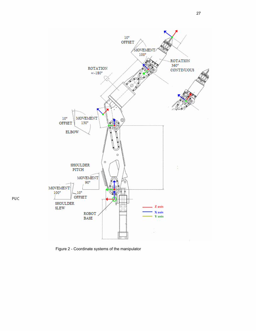
Homogeneous transformations represent a suitable way to describe
translations and rotations simultaneously. The different reference frames
(coordinate systems) in the respective joints of the manipulator TA-40 studied in
this work, are shown in Figure 2. The relative translation and orientation of every
joint can be described by a 4x4 homogeneous matrix. Eventually, the coordinates
of the end effector relative to the manipulator base can be calculated by
multiplying all the transformation matrices representing the respective joints.
This chapter is organized in the following way: Section 2.2 describes the
basic concepts of kinematics necessary to model a manipulator. Section 2.3
describes the Denavit-Hartenberg notation (DH) that is used to model the TA-40.
Section 2.4 describes the techniques used to calibrate the manipulator. Section 2.5
deduces the inverse kinematics for the manipulator.
27
Figure 2 - Coordinate systems of the manipulator
28
2.2. Basic Concepts of Kinematics
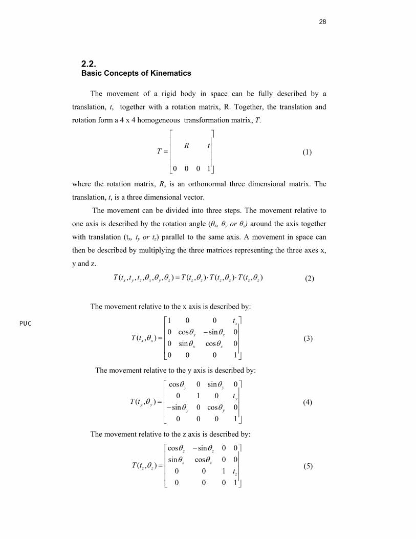
The movement of a rigid body in space can be fully described by a
translation, t, together with a rotation matrix, R. Together, the translation and
rotation form a 4 x 4 homogeneous transformation matrix, T.
0 0 0 1
R tT
⎡ ⎤⎢ ⎥⎢ ⎥=⎢ ⎥⎢ ⎥⎣ ⎦
(1)
where the rotation matrix, R, is an orthonormal three dimensional matrix. The
translation, t, is a three dimensional vector.
The movement can be divided into three steps. The movement relative to
one axis is described by the rotation angle (θx, θy or θz) around the axis together
with translation (tx, ty or tz) parallel to the same axis. A movement in space can
then be described by multiplying the three matrices representing the three axes x,
y and z.
( , , , , , ) ( , ) ( , ) ( , )x y z x y z z z z z z zT t t t T t T t T tθ θ θ θ θ θ= ⋅ ⋅ (2)
The movement relative to the x axis is described by:
1 0 00 cos sin 0
( , )0 sin cos 00 0 0 1
x
x xx x
x x
t
T tθ θ
θθ θ
⎡ ⎤⎢ ⎥−⎢ ⎥=⎢ ⎥⎢ ⎥⎣ ⎦
(3)
The movement relative to the y axis is described by:
cos 0 sin 00 1 0
( , )sin 0 cos 0
0 0 0 1
y y
yy y
y y
tT t
θ θ
θθ θ
⎡ ⎤⎢ ⎥⎢ ⎥=⎢ ⎥−⎢ ⎥⎣ ⎦
(4)
The movement relative to the z axis is described by:
cos sin 0 0sin cos 0 0
( , )0 0 10 0 0 1
z z
z zz z
z
T tt
θ θθ θ
θ
−⎡ ⎤⎢ ⎥⎢ ⎥=⎢ ⎥⎢ ⎥⎣ ⎦
(5)
29
2.3. The Denavit-Hartenberg Convention
The Denavit-Hartenberg notation uses a homogeneous transformation (4 x 4
matrix) to describe the kinematic relationship between a pair of adjacent links.
The transformation matrix between the end-effector and the robot base is found by
multiplying all the matrices representing the different links and joints. The
notation represents a slight simplification of a full 3D movement. It only
considers the movements along the x and z axes giving the two adjacent reference
frames a common normal along the x axis. The common normals are parallel
when θi = 0°.
Figure 3 shows a pair of adjacent links, link i-1 and link i, and their
associated joints, joint i+1 and joint i. The line iiOH is called the common
normal between the axis i and i+1. The two joints represent two different
coordinate systems. In the DH notation, the origin of coordinate system number i
is situated in the intersection between axis i+1 and the common normal between
the joints i and i+1, as shown in figure 3.
The origin of the i-th coordinate frame Oi is located at the intersection of
joints axis i+1 and the common normal between joint axes i and i+1, as shown in
figure 3. The frame of link i is at joint i+1 rather than at joint i. The xi axis is
directed along the extension line of the common normal. The zi axis is along the
joint axis i+1. The yi axis is chosen according to the right-hand rule.
30
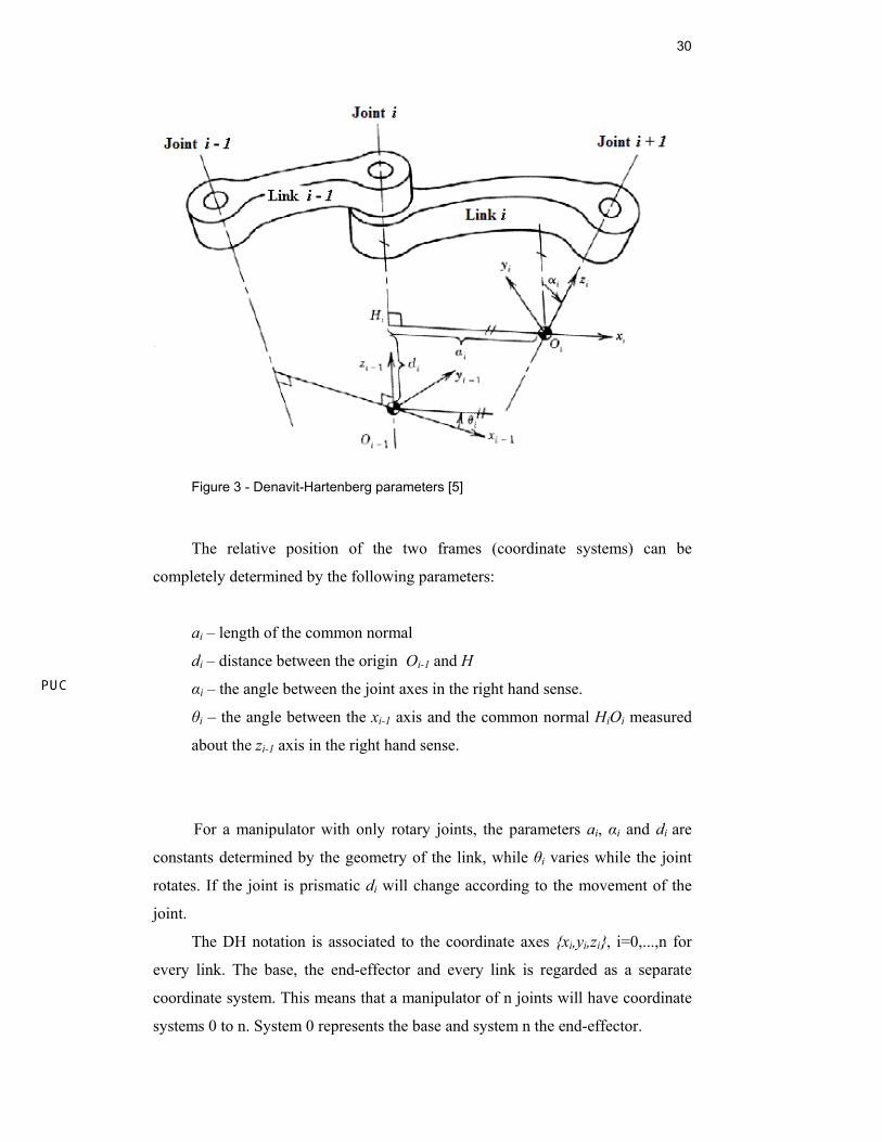
Figure 3 - Denavit-Hartenberg parameters [5]
The relative position of the two frames (coordinate systems) can be
completely determined by the following parameters:
ai – length of the common normal
di – distance between the origin Oi-1 and H
αi – the angle between the joint axes in the right hand sense.
θi – the angle between the xi-1 axis and the common normal HiOi measured
about the zi-1 axis in the right hand sense.
For a manipulator with only rotary joints, the parameters ai, αi and di are
constants determined by the geometry of the link, while θi varies while the joint
rotates. If the joint is prismatic di will change according to the movement of the
joint.
The DH notation is associated to the coordinate axes {xi,yi,zi}, i=0,...,n for
every link. The base, the end-effector and every link is regarded as a separate
coordinate system. This means that a manipulator of n joints will have coordinate
systems 0 to n. System 0 represents the base and system n the end-effector.
31
The transformation matrix from the end-effector to the base coordinates is
given by Eq. (6) 0 0 1 0 1 1
1 2 1 ... ....i nn i nT A A A A A− −= (6)
where 1iiA − is the homogeneous transformation matrix between coordinate system
i-1 relative to coordinate system i.
The transformation of coordinates 1iiA − is therefore represented by its 4
parameters (θi, ai, di, αi ). The construction of the matrices Ai for the links
i=1,2,...,n-1 is shown. If the i-th joint is revolute, the following transformations
are necessary to transform the i+1 to the system i.
The coordinate transformation is done in 4 steps which together constitute
the Denavit-Hartenberg transformation matrix:
• Rotate the (i-1)-th coordinate system around the xi axis by an angle αi
• Translate the coordinate system a distance di along the zi-1 axis so that the
origin of the moving system reaches the intersection between the common
normal and normal of the i-th joint.
• Translate the coordinate system a distance ai along the xi axis.
• Rotate the coordinate system i-1 around the axis zi-1 an angle θi, so that the
x axis of the moving coordinate system is parallel xi axis.
The transformation matrix is then found by multiplying the movements along the
x axis and the z axis:
1
cos sin 0 0 1 0 0sin cos 0 0 0 cos sin 0
0 0 1 0 sin cos 00 0 0 1 0 0 0 1
i
i i i
i i i iiz x
i i i
a
A T Td
θ θθ θ α α
α α−
−⎡ ⎤ ⎡ ⎤⎢ ⎥ ⎢ ⎥−⎢ ⎥ ⎢ ⎥= ⋅ = ⋅⎢ ⎥ ⎢ ⎥⎢ ⎥ ⎢ ⎥⎣ ⎦ ⎣ ⎦
(7)
Giving the transformation matrix between each joint:
32
1
cos sin cos sin sin cossin cos cos cos sin sin
0 sin cos0 0 0 1
i i i i i i i
i i i i i i iii
i i i
aa
Ad
θ θ α θ α θθ θ α θ α θ
α α−
−⎡ ⎤⎢ ⎥−⎢ ⎥=⎢ ⎥⎢ ⎥⎣ ⎦
(8)
2.4. Classic Manipulator Calibration
By applying the nominal measurements of the manipulator in the DH
notation, it is possible to estimate the approximate position and orientation of the
manipulator end-effector. In order to increase the precision of the manipulator an
error model has to be introduced. The errors are then found by calibration.
The method used will only find the repetitive errors in the robot frame.
These errors are caused by precision errors in the fabrication of the manipulator,
meaning that the nominal values of the links and joints deviate from the actual
ones. These errors do not include play in the joints or other random errors that
might occur.
To model the repetitive errors, a notation called generalized errors model
will be used. It consists of a homogeneous matrix with 6 parameters. The error
matrices are multiplied to the transformation matrices of the DH notation to
estimate the effect of the errors in the joints and links.
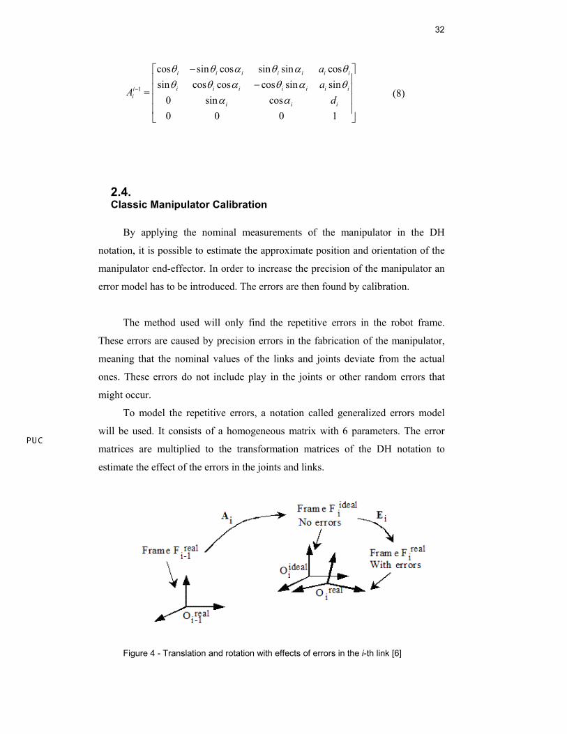
Figure 4 - Translation and rotation with effects of errors in the i-th link [6]
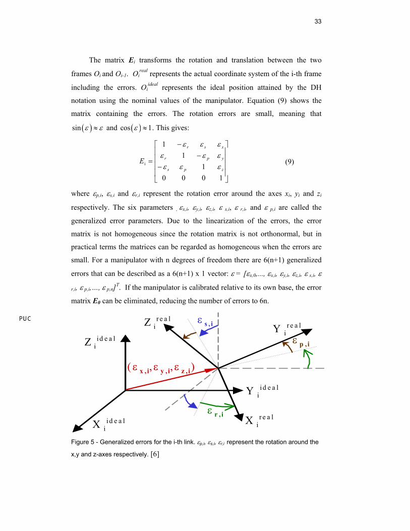
33
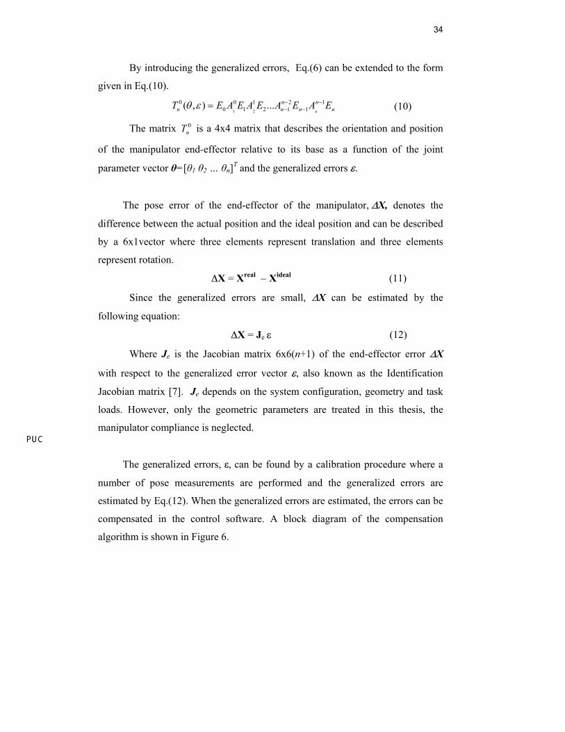
The matrix Ei transforms the rotation and translation between the two
frames Oi and Oi-1. Oireal represents the actual coordinate system of the i-th frame
including the errors. Oiideal represents the ideal position attained by the DH
notation using the nominal values of the manipulator. Equation (9) shows the
matrix containing the errors. The rotation errors are small, meaning that
( )sin ε ε≈ and ( )cos 1ε ≈ . This gives:
⎥⎥⎥⎥
⎦
⎤
⎢⎢⎢⎢
⎣
⎡
−−
−
=
10001
11
izps
ypr
xsr
Eεεεεεεεεε
(9)
where εp,i, εs,i and εr,i represent the rotation error around the axes xi, yi and zi
respectively. The six parameters , εx,i, εy,i, εz,i, ε s,i, ε r,i, and ε p,i are called the
generalized error parameters. Due to the linearization of the errors, the error
matrix is not homogeneous since the rotation matrix is not orthonormal, but in
practical terms the matrices can be regarded as homogeneous when the errors are
small. For a manipulator with n degrees of freedom there are 6(n+1) generalized
errors that can be described as a 6(n+1) x 1 vector: ε = [εx,0,..., εx,i, εy,i, εz,i, ε s,i, ε
r,i, ε p,i,…, ε p,n]T. If the manipulator is calibrated relative to its own base, the error
matrix E0 can be eliminated, reducing the number of errors to 6n.
ε s , i
ε p ,i
ε r , iX i
id e a l
Y iid e a l
Z iid e a l
X ir e a l
Y ir e a lZ i
r e a l
( ε x , i , ε y , i , ε z , i)
Figure 5 - Generalized errors for the i-th link. εp,i, εs,i, εr,i represent the rotation around the
x,y and z-axes respectively. [6]
34
By introducing the generalized errors, Eq.(6) can be extended to the form
given in Eq.(10).
1 2
0 0 1 2 10 1 2 1 1( , ) ...
n
n nn n n nT E A E A E A E A Eθ ε − −
− −= (10)
The matrix 0nT is a 4x4 matrix that describes the orientation and position
of the manipulator end-effector relative to its base as a function of the joint
parameter vector θ=[θ1 θ2 … θn]T and the generalized errors ε.
The pose error of the end-effector of the manipulator, ∆X, denotes the
difference between the actual position and the ideal position and can be described
by a 6x1vector where three elements represent translation and three elements
represent rotation.
∆X = Xreal − Xideal (11)
Since the generalized errors are small, ∆X can be estimated by the
following equation:
∆X = Je ε (12)
Where Je is the Jacobian matrix 6x6(n+1) of the end-effector error ∆X
with respect to the generalized error vector ε, also known as the Identification
Jacobian matrix [7]. Je depends on the system configuration, geometry and task
loads. However, only the geometric parameters are treated in this thesis, the
manipulator compliance is neglected.
The generalized errors, ε, can be found by a calibration procedure where a
number of pose measurements are performed and the generalized errors are
estimated by Eq.(12). When the generalized errors are estimated, the errors can be
compensated in the control software. A block diagram of the compensation
algorithm is shown in Figure 6.
35
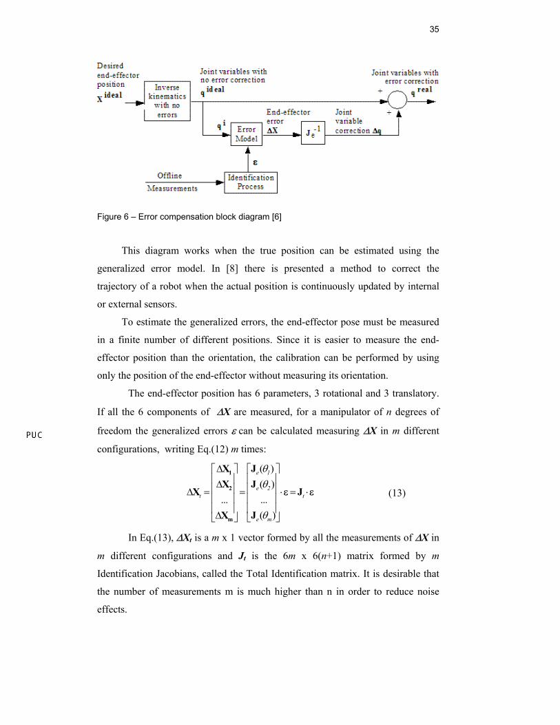
Figure 6 – Error compensation block diagram [6]
This diagram works when the true position can be estimated using the
generalized error model. In [8] there is presented a method to correct the
trajectory of a robot when the actual position is continuously updated by internal
or external sensors.
To estimate the generalized errors, the end-effector pose must be measured
in a finite number of different positions. Since it is easier to measure the end-
effector position than the orientation, the calibration can be performed by using
only the position of the end-effector without measuring its orientation.
The end-effector position has 6 parameters, 3 rotational and 3 translatory.
If all the 6 components of ∆X are measured, for a manipulator of n degrees of
freedom the generalized errors ε can be calculated measuring ∆X in m different
configurations, writing Eq.(12) m times:
( )( )......( )
1
2
m
JXJX
X J JX
e 1
e 2t t
e m
θθ
θ
∆ ⎡ ⎤⎡ ⎤⎢ ⎥⎢ ⎥∆ ⎢ ⎥⎢ ⎥∆ = = ⋅ = ⋅⎢ ⎥⎢ ⎥⎢ ⎥⎢ ⎥∆⎣ ⎦ ⎣ ⎦
ε ε (13)
In Eq.(13), ∆Xt is a m x 1 vector formed by all the measurements of ∆X in
m different configurations and Jt is the 6m x 6(n+1) matrix formed by m
Identification Jacobians, called the Total Identification matrix. It is desirable that
the number of measurements m is much higher than n in order to reduce noise
effects.
36
When the errors are constant, the least square estimate of ε can be calculated
by Eq.(14).
( ) 1ε ∆= ⋅
−J J J Xt
Tt t
Tt (14)
Unfortunately, the Identification Jacobian matrix usually contains columns
that are linearly dependent. Therefore Eq. (14) will achieve poor accuracy due to
poor matrix conditioning [7]. This occurs when some of the generalized errors are
redundant, meaning that it is not possible to distinguish each error’s influence on
the end-effector position.
2.5. Elimination of Redundant Errors
In order to solve Eq.(14), all the linearly dependent errors have to be
eliminated. Here a detailed explanation of the elimination procedure will be
given.
The columns , Jx,i, Jy,i, Jz,i, Js,i, Jr,i and Jp,i, of Je are associated to each of
the generalized errors εx,i, εy,i, εz,i, εs,i, εr,i and εp,i, respectively. Equation (12) can
be written in the form:
,0
,
,
,,0 , , , , , , ,
,
,
,
,
...
... ...
...
x
x i
y i
z ix x i y i z i s i r i p i p n
s i
r i
p i
p n
X J J J J J J J J
ε
εεεεεε
ε
⎡ ⎤⎢ ⎥⎢ ⎥⎢ ⎥⎢ ⎥⎢ ⎥⎢ ⎥
⎡ ⎤ ⎢ ⎥∆ = ⎣ ⎦ ⎢ ⎥⎢ ⎥⎢ ⎥⎢ ⎥⎢ ⎥⎢ ⎥⎢ ⎥⎣ ⎦
(15)
For each link i, i between 1 and n, the following linear combinations are
always valid for a manipulator described by the DN notation [6]:
i,zii,yi)1(i,z cossin JJJ α+α≡− (16)
i,rii,sii,ziii,yii)1,(ir cossinsinacosa JJJJJ α+α+α−α≡− (17)
37
If joint i is prismatic, then additional combinations of the columns of Je are
valid:
i,x)1(i,x JJ ≡− (18)
i,zii,yi)1(i,y sincos JJJ α−α≡− (19)
The linear combinations shown above are always valid, independently of
the values of ai and αi. If both position and orientation are measured, then
Equations (16)-(19) are the only linear combinations for link i.
To obtain the non-singular Identification Jacobian matrix, called here Ge,
columns Jz,(i-1) and Jr,(i-1) must be eliminated from the matrix Je for all values of i
between 1 and n. If joint i is prismatic, then columns Jx,(i-1) and Jy,(i-1) must also
be eliminated. For an n DOF (Degrees Of Freedom) manipulator with r rotary
joints and p (p equal to n-r) prismatic joints, a total of 2r+4p columns are
eliminated from the Identification Jacobian Je to form its submatrix Ge. This
means that 2r+4p generalized errors cannot be obtained by measuring the end-
effector position.
The dependent error parameters eliminated from ε do not affect the end-
effector error, resulting in the identity:
∆X = Je ε ≡ Ge ε· (20)
Using the above identity and the linear combinations of the columns of Je
from Eqs.(16)-(19), it is possible to obtain all relationships between the
generalized error set ε and its independent subset, ε·. If joint i is revolute (i
between 1 and n), then the generalized errors εz,(i-1) and εr,(i-1) are eliminated, and
its values are incorporated into the independent error parameters ε∗y,i, ε∗
z,i, ε∗s,i and
ε∗r,i :
⎪⎪⎩
⎪⎪⎨
⎧
αε+ε≡εαε+ε≡ε
α⋅ε−αε+ε≡εα⋅ε+αε+ε≡ε
−
−
−−
−−
i)1i(,ri,r*
i,r
i)1i(,ri,s*
i,s
ii)1i(,ri)1i(,zi,z*
i,z
ii)1i(,ri)1i(,zi,y*
i,y
cossin
sinacoscosasin
(21)
If joint i is prismatic, then the translational errors εx,(i-1) and εy,(i-1) are
eliminated, and their values are incorporated into the independent error parameters
ε∗x,i, ε∗
y,i and ε∗z,i. In this case, Eq.(21) becomes:
38
⎪⎪⎪
⎩
⎪⎪⎪
⎨
⎧
αε+ε≡εαε+ε≡ε
α⋅ε−αε+αε−ε≡εα⋅ε+αε+αε+ε≡ε
ε+ε≡ε
−
−
−−−
−−−
−
i)1i(,ri,r*
i,r
i)1i(,ri,s*
i,s
ii)1i(,ri)1i(,zi)1i(,yi,z*
i,z
ii)1i(,ri)1i(,zi)1i(,yi,y*
i,y
)1i(,xi,x*
i,x
cossin
sinacossincosasincos
(22)
If the vector ε· containing the independent errors is constant, then the matrix
Ge can be used to replace Je in Eq.(20), and Eq.(22) is applied to calculate the
estimate of the independent generalized errors ε·, completing the identification
process. However, if non-geometric factors are considered, then it is necessary to
further model the parameters of ε· as a function of the system configuration prior
to the identification process.
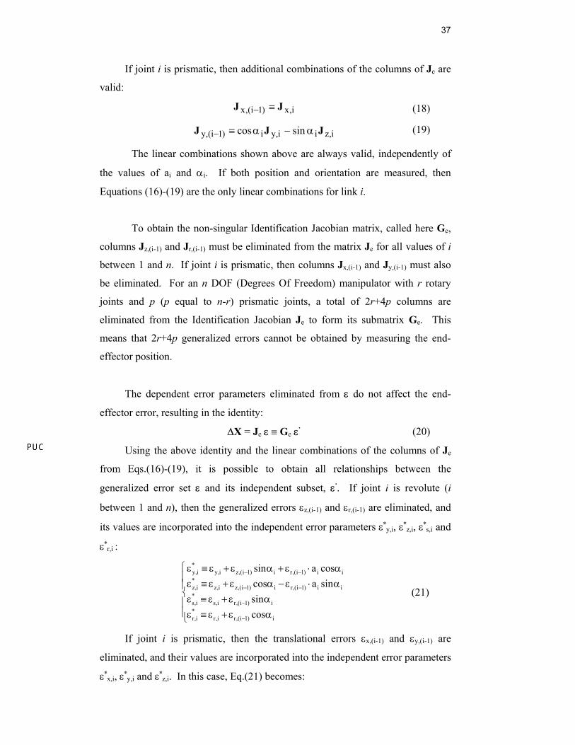
2.6. Physical Interpretation of the Redundant Errors
To fully understand the concepts of redundant errors it is a good idea to
develop a geometric interpretation.
Equation (16) shows that a translation along the z(i-1) axis provokes the
same translation error on the end effector as a combination of 2 errors in z and y
direction of the joint zi. This principle is shown in figure 7.
αi εz,iεy,iεz,(i-1)
Figure 7 – Combination of translational linear errors [6]
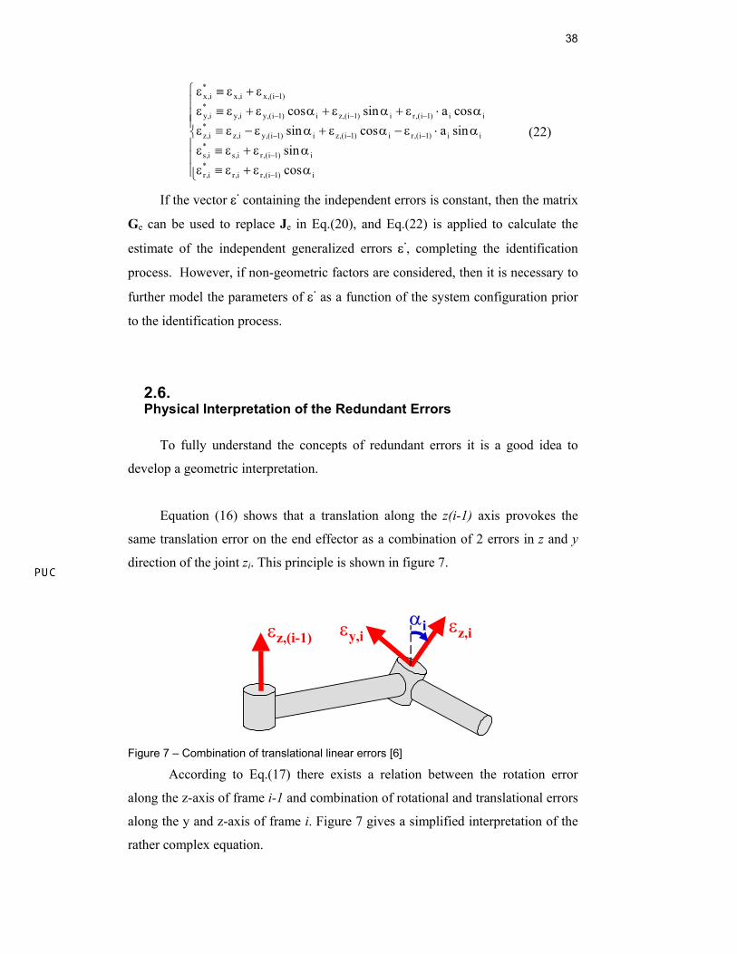
According to Eq.(17) there exists a relation between the rotation error
along the z-axis of frame i-1 and combination of rotational and translational errors
along the y and z-axis of frame i. Figure 7 gives a simplified interpretation of the
rather complex equation.
39
.
εr,(i-1)
εr,i
εy,i
∆Xr
∆Xr
∆Xt
∆Xt
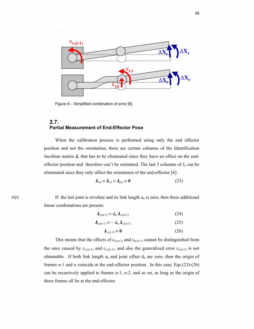
Figure 8 – Simplified combination of error [6]
2.7. Partial Measurement of End-Effector Pose
When the calibration process is performed using only the end effector
position and not the orientation, there are certain columns of the Identification
Jacobian matrix Je that has to be eliminated since they have no effect on the end-
effector position and therefore can’t be estimated. The last 3 columns of Je can be
eliminated since they only affect the orientation of the end-effector [6]:
Js,n ≡ Jr,n ≡ Jp,n ≡ 0 (23)
If the last joint is revolute and its link length an is zero, then three additional
linear combinations are present:
Js,(n-1) ≡ dn Jx,(n-1) (24)
Jp,(n-1) ≡ − dn Jy,(n-1) (25)
Jr,(n-1) ≡ 0 (26)
This means that the effects of εs,(n-1) and εp,(n-1) cannot be distinguished from
the ones caused by εx,(n-1) and εy,(n-1), and also the generalized error εr,(n-1) is not
obtainable. If both link length an and joint offset dn are zero, then the origin of
frames n-1 and n coincide at the end-effector position. In this case, Eqs.(23)-(26)
can be recursively applied to frames n-1, n-2, and so on, as long as the origin of
these frames all lie at the end-effector.
40
When only an is zero, εs,(n-1) and εy,(n-1) can be eliminated and their values
transferred to εx,(n-1) and εp,(n-1) respectively shown in Eq.(27):
⎪⎩
⎪⎨⎧
⋅ε−ε=ε
⋅ε+ε=ε
−−−
−−−
n1)(n,p1)(n,y*
1)(n,y
n1)(n,s1)(n,x*
1)(n,x
d
d
(27)
2.8. Inverse Kinematics
Through the Denavit-Hartenberg notation the direct kinematics of the
manipulator is obtained, where the orientation and position of the end-effector is
estimated using the angles of all joints as inputs.
Inverse kinematics uses the DN-notation to generate the required angles of
the joints to reach the desired position and orientation. In order to be able to
automate certain tasks, finding the inverse kinematics is a necessary step.
The inverse kinematics is generally more complex than direct kinematics,
and there exist several solutions for the same desired position. For some positions
there might not be any solution at all. Due to the non-linearity of the equations it
is difficult to elaborate a general solution. Every case has to be estimated
individually from the direct kinematic equations. If an analytical solution is not
found, it might be found by numerical methods.
In order to be able to reach any desired position and orientation, the
manipulator needs at least six degrees of freedom. Manipulators with less degrees
of freedom will not be able to reach an arbitrary position in 3D space. If a
manipulator has more than six degrees of freedom, there may be an infinite
number of possible solutions for every position.
2.8.1. Solvability
In cases where an analytical solution for the inverse kinematics does not
exist, iterative numerical solutions there can be implemented. This is generally
computationally heavy. An analytical solution is therefore desirable whenever
possible.
41
The existence of an analytical solution depends on the kinematic structure of
the manipulator. The structure is usually designed in order to achieve this, so that
complex calculations can be avoided.
Reference [10] shows that having three rotational consecutive joints whose
axes intersect in one single point for all configurations of the joints is enough to
guarantee an analytical solution for a manipulator with six degrees of freedom.
This is the case for the manipulator studied in this work. The axes of the joints 4,
5 and 6 intersect at the origin of joints 4 and 5.
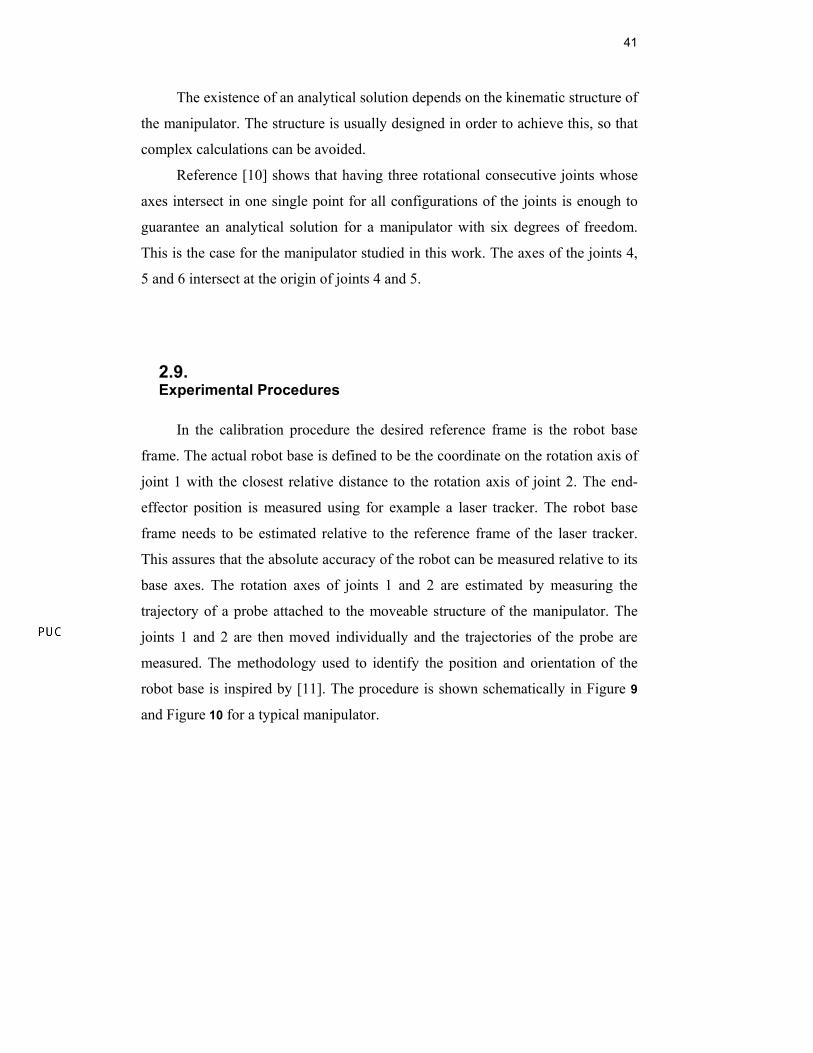
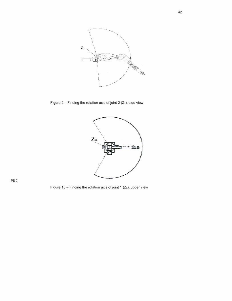
2.9. Experimental Procedures
In the calibration procedure the desired reference frame is the robot base
frame. The actual robot base is defined to be the coordinate on the rotation axis of
joint 1 with the closest relative distance to the rotation axis of joint 2. The end-
effector position is measured using for example a laser tracker. The robot base
frame needs to be estimated relative to the reference frame of the laser tracker.
This assures that the absolute accuracy of the robot can be measured relative to its
base axes. The rotation axes of joints 1 and 2 are estimated by measuring the
trajectory of a probe attached to the moveable structure of the manipulator. The
joints 1 and 2 are then moved individually and the trajectories of the probe are
measured. The methodology used to identify the position and orientation of the
robot base is inspired by [11]. The procedure is shown schematically in Figure 9
and Figure 10 for a typical manipulator.
42
Figure 9 – Finding the rotation axis of joint 2 (Z1), side view
Figure 10 – Finding the rotation axis of joint 1 (Z0), upper view
43
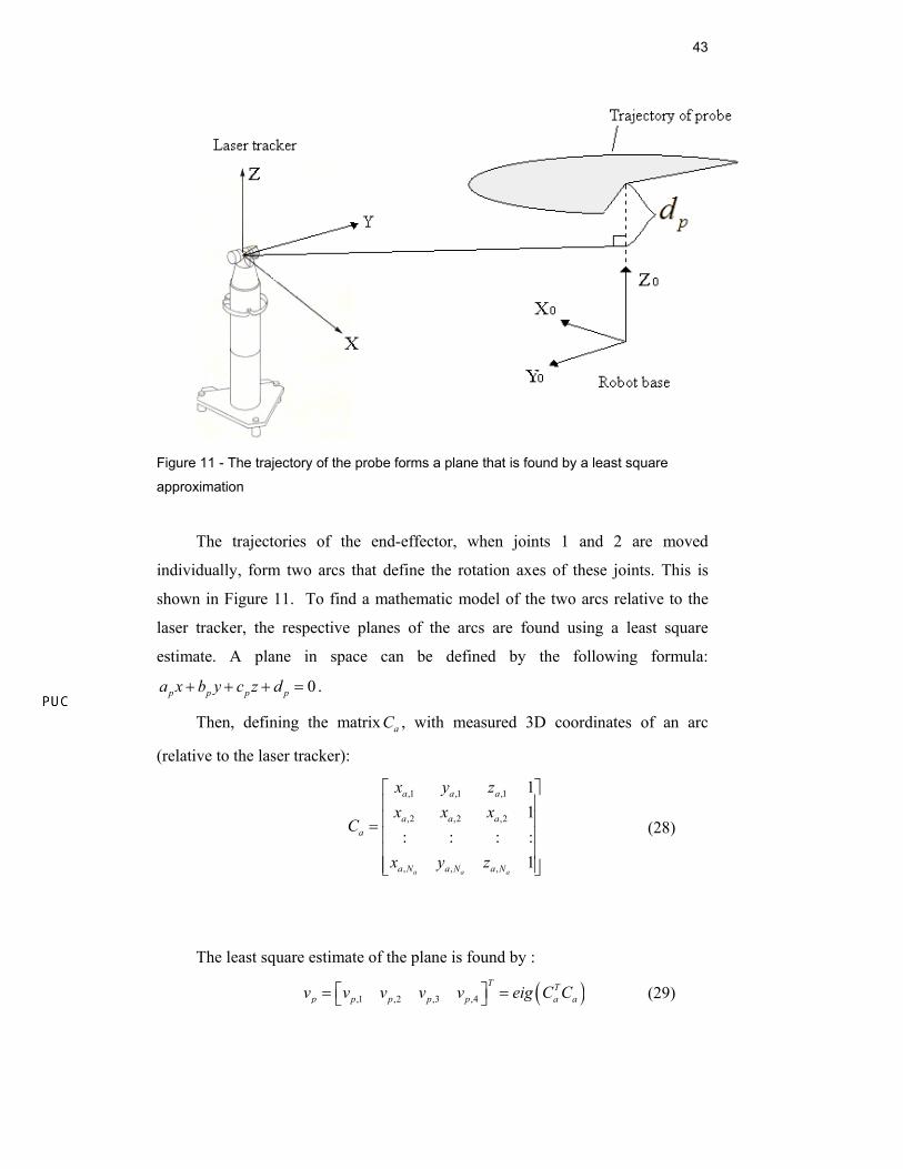
Figure 11 - The trajectory of the probe forms a plane that is found by a least square
approximation
The trajectories of the end-effector, when joints 1 and 2 are moved
individually, form two arcs that define the rotation axes of these joints. This is
shown in Figure 11. To find a mathematic model of the two arcs relative to the
laser tracker, the respective planes of the arcs are found using a least square
estimate. A plane in space can be defined by the following formula:
0p p p pa x b y c z d+ + + = .
Then, defining the matrix aC , with measured 3D coordinates of an arc
(relative to the laser tracker):
,1 ,1 ,1
,2 ,2 ,2
, , ,
11
: : : :1
a a a
a a a
a a aa
a N a N a N
x y zx x x
C
x y z
⎡ ⎤⎢ ⎥⎢ ⎥=⎢ ⎥⎢ ⎥⎢ ⎥⎣ ⎦
(28)
The least square estimate of the plane is found by :
( ),1 ,2 ,3 ,4
T Tp p p p p a av v v v v eig C C⎡ ⎤= =⎣ ⎦ (29)
44
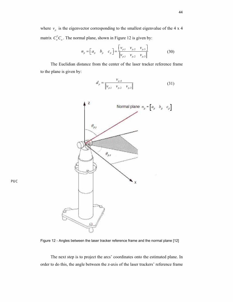
where pv is the eigenvector corresponding to the smallest eigenvalue of the 4 x 4
matrix Ta aC C . The normal plane, shown in Figure 12 is given by:
,1 ,2 ,3
,1 ,2 ,3
p p pp p p p
p p p
v v vn a b c
v v v
⎡ ⎤⎣ ⎦⎡ ⎤= =⎣ ⎦ (30)
The Euclidian distance from the center of the laser tracker reference frame
to the plane is given by:
,4
,1 ,2 ,3
pp
p p p
vd
v v v= (31)
Figure 12 - Angles between the laser tracker reference frame and the normal plane [12]
The next step is to project the arcs’ coordinates onto the estimated plane. In
order to do this, the angle between the z-axis of the laser trackers’ reference frame
45
and the normal plane is estimated. The rotation angle around the y-axis is given
by:
( )1, cosp y pcθ −= (32)
where 1cos− is the arc cosine function. The rotation around the z-axis is given by.
1, tan p
p zp
ba
θ −⎛ ⎞
= ⎜ ⎟⎜ ⎟⎝ ⎠
(33)
The rotation matrix between the normal plane and the laser trackers’ z-axis
is then given by:
( ) ( )( ) ( )
( ) ( )
( ) ( )
, , , ,
, ,
, ,
cos sin 0 cos 0 sin
sin cos 0 0 1 0
sin 0 cos0 0 1
p z p z p y p y
p p z p z
p y p y
R
θ θ θ θ
θ θ
θ θ
⎡ ⎤− ⎡ ⎤⎢ ⎥ ⎢ ⎥⎢ ⎥= ⋅ ⎢ ⎥⎢ ⎥ ⎢ ⎥
−⎢ ⎥ ⎢ ⎥⎣ ⎦⎣ ⎦
(34)
To find the rotation center of the arc, the coordinate matrix aC is projected
onto the estimated plane, creating the projected coordinate set `aC .
( )` TT Ta p aC R C= (35)
The new set of coordinates is given relative to the laser tracker, but the
reference z-axis is transformed so that it is parallel to the estimated normal plane.
This gives the same z-value for all the coordinates. The rotation center of the arc
can then be estimated using the x and y coordinates. To estimate the rotation
center in the plane, a circle is fitted using the projected coordinates. The circle is
fitted using a least square estimate proposed in [13]. This method is much simpler
to implement than the iterative Levenberg-Marquardt method used in [11].
The x and y coordinates of `aC are extracted. Defining the x coordinates as
`ax and the y coordinates as `
ay .
Having a set of 2D coordinates, `ax and `
ay represent the trajectory of the
probe projected onto the estimated plane. The mean of the coordinates,
respectively, is given by: ___ ___
` ` `, ,
1 1
1 1, p pN N
a a i a ipi ip p
x x y xN N= =
= =∑ ∑ (36)
where Np is the number of measured samples.
46
Introducing the translated variables: __
` `t a ax x x= − (37)
and __
` `t a ay y y= − (38)
The observation matrix is given by:
,1 ,1
, ,
2 2 1: : :
2 2 1p p
t t
t
t N t N
x xC
x y
⎡ ⎤−⎢ ⎥
= ⎢ ⎥⎢ ⎥−⎣ ⎦
(39)
The vector ob is given by:
2 2
1 1
2 2
:
p p
t t
t
tN tN
x yb
x y
⎡ ⎤+⎢ ⎥
= ⎢ ⎥⎢ ⎥+⎣ ⎦
(40)
Let the vector u be the least square solution to the problem A u b⋅ = giving:
( ) 1t tT T
t t tu C C C b−
= ⋅ ⋅ (41)
So tu is then a 3 x 1 vector: [ ]1 2 3T
tu u u u= .
Defining xr and yr as the coordinates of the circle center, and rr as the radius
of the circle. They are given by the following equations:
1rx u= (42)
2ry u= (43)
2 23r r rr x y u= + − (44)
The rotation center of the joint relative to the laser tracker is then given by: T
r p r r pc R x y d⎡ ⎤= ⋅ ⎣ ⎦ (45)
Estimating the rotation center and normal plane for both the joints 1 and 2,
the actual robot base can be found using the triangulation method shown in
section 3.5.
3 Computer Vision
3.1. Introduction
The TA-40 manipulator studied in this work is attached to a ROV (Remote
Operating Vehicle) that takes it to its work environment. Every time it reaches its
work position, the relative position of the manipulator base needs to be calibrated
before the end-effector position can be estimated relative to the work
environment. The primary goal of this thesis is to find a way to estimate this
position by the use of digital cameras mounted on the manipulator.
Any form of automation requires that the robot is capable of finding its
position in the environment. When the position is estimated, the operator can get a
feed-back by means of virtual reality that can give a more detailed and
comprehensive overview of the work environment. Through the use of the inverse
kinematic model certain tasks can also be automated.
In this chapter, the mathematic camera model will be described, as well as
how the parameters are obtained through calibration. Then a description will be
given about how features are extracted from the images and how they are
recognized in other images.
48
3.2. Mathematic Camera Models
3.2.1. The Pinhole Model
The pinhole model is one of the simplest and most widely used camera
models. It is very useful in computer vision, due to its simple linear geometric
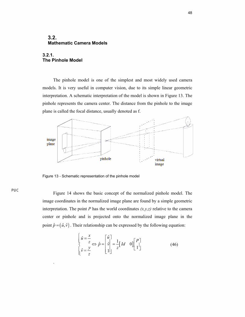
interpretation. A schematic interpretation of the model is shown in Figure 13. The
pinhole represents the camera center. The distance from the pinhole to the image
plane is called the focal distance, usually denoted as f.
Figure 13 - Schematic representation of the pinhole model
Figure 14 shows the basic concept of the normalized pinhole model. The
image coordinates in the normalized image plane are found by a simple geometric
interpretation. The point P has the world coordinates (x,y,z) relative to the camera
center or pinhole and is projected onto the normalized image plane in the
point ( )ˆ ˆ ˆ,p u v= . Their relationship can be expressed by the following equation:
[ ]ˆˆ
1ˆ ˆ 01ˆ 1
x uu Pz p v Idy zvz
⎧ ⎡ ⎤=⎪ ⎡ ⎤⎪ ⎢ ⎥⇔ = =⎨ ⎢ ⎥⎢ ⎥ ⎣ ⎦⎪ = ⎢ ⎥⎣ ⎦⎪⎩
(46)
.
49
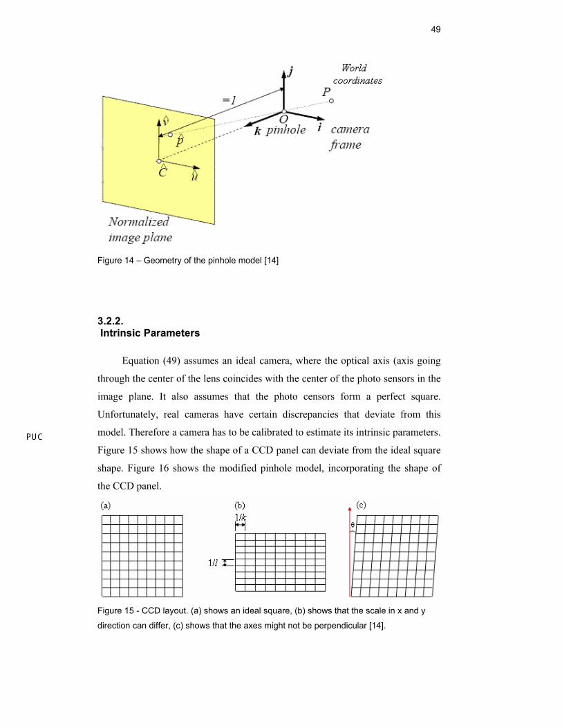
Figure 14 – Geometry of the pinhole model [14]
3.2.2. Intrinsic Parameters
Equation (49) assumes an ideal camera, where the optical axis (axis going
through the center of the lens coincides with the center of the photo sensors in the
image plane. It also assumes that the photo censors form a perfect square.
Unfortunately, real cameras have certain discrepancies that deviate from this
model. Therefore a camera has to be calibrated to estimate its intrinsic parameters.
Figure 15 shows how the shape of a CCD panel can deviate from the ideal square
shape. Figure 16 shows the modified pinhole model, incorporating the shape of
the CCD panel.
Figure 15 - CCD layout. (a) shows an ideal square, (b) shows that the scale in x and y
direction can differ, (c) shows that the axes might not be perpendicular [14].
50
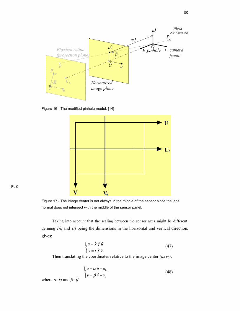
Figure 16 - The modified pinhole model. [14]
Figure 17 - The image center is not always in the middle of the sensor since the lens
normal does not intersect with the middle of the sensor panel.
Taking into account that the scaling between the sensor axes might be different,
defining 1/k and 1/l being the dimensions in the horizontal and vertical direction,
gives:
(47)
Then translating the coordinates relative to the image center (u0,v0):
where α=kf and β=lf
(48) ⎩⎨⎧
+=+=
0
0
ˆˆ
vvvuuu
βα
⎩⎨⎧
==
vflvufkuˆˆ
51
Taking into account that the sensors can be distorted by an angle θ, gives:
(49)
All these intrinsic parameters define the calibration matrix of the camera
which relates the actual image coordinates, p, with the ideal normalized
coordinates, p .
0
0
ˆcotˆˆ0 / sin
1 0 0 1 1
u u uv v v κ
α α θβ θ−⎛ ⎞ ⎛ ⎞⎛ ⎞
⎜ ⎟ ⎜ ⎟⎜ ⎟= = =⎜ ⎟ ⎜ ⎟⎜ ⎟⎜ ⎟ ⎜ ⎟⎜ ⎟⎝ ⎠ ⎝ ⎠⎝ ⎠
p p (50)
Estimating the normalized pinhole coordinates is important in computer
vision since they give the true line of sight to any object in the image. The
normalized image coordinates can then be found by: ^
1p К p−= (51)
3.2.3. Extrinsic Parameters
The previous section described how an object with known coordinates
relative to the camera center is projected onto image plane. Often the coordinates
of an object are given with respect to another reference frame than the actual
camera center. Therefore, it is necessary to estimate how the other reference frame
is expressed in terms of the camera reference frame. Figure 18 shows a schematic
interpretation of the two reference frames.
⎩⎨⎧
+=+−=
0
0
ˆˆθcotˆ
vvvuvuu
βαα
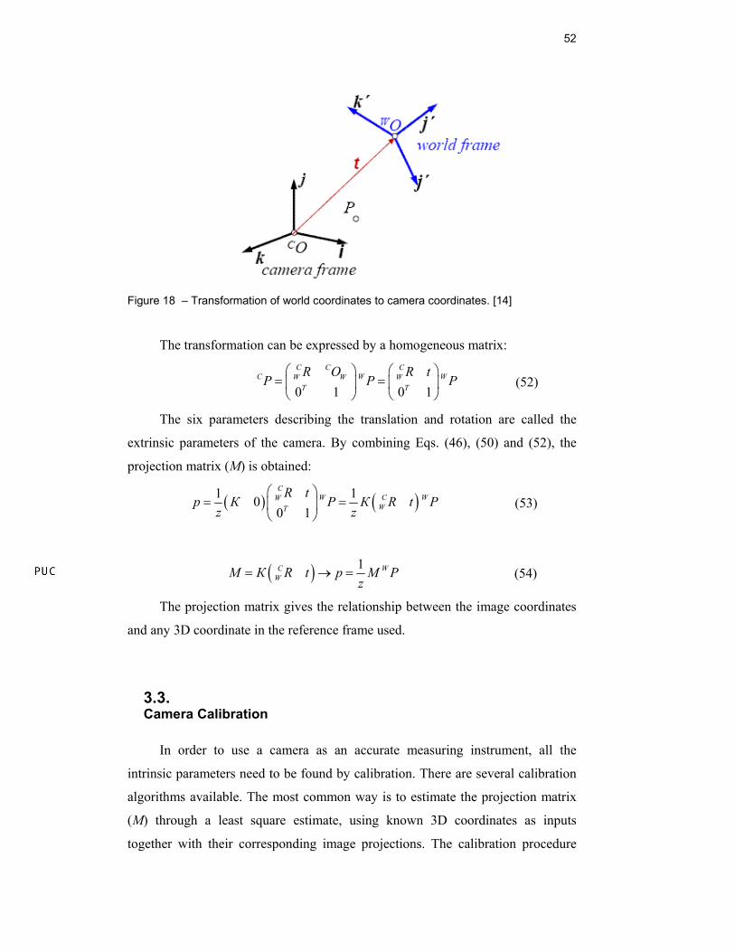
52
Figure 18 – Transformation of world coordinates to camera coordinates. [14]
The transformation can be expressed by a homogeneous matrix:
0 1 0 1
C C CC W WW W W
T T
R O R tP P P
⎛ ⎞ ⎛ ⎞= =⎜ ⎟ ⎜ ⎟⎝ ⎠ ⎝ ⎠
(52)
The six parameters describing the translation and rotation are called the
extrinsic parameters of the camera. By combining Eqs. (46), (50) and (52), the
projection matrix (M) is obtained:
( ) ( )1 100 1
CW C WW
WT
R tp К P К R t P
z z⎛ ⎞
= =⎜ ⎟⎝ ⎠
(53)
( ) 1C WWM К R t p M P
z= → = (54)
The projection matrix gives the relationship between the image coordinates
and any 3D coordinate in the reference frame used.
3.3. Camera Calibration
In order to use a camera as an accurate measuring instrument, all the
intrinsic parameters need to be found by calibration. There are several calibration
algorithms available. The most common way is to estimate the projection matrix
(M) through a least square estimate, using known 3D coordinates as inputs
together with their corresponding image projections. The calibration procedure
53
used to find the intrinsic parameters for the pin-hole model in this thesis is based
on the method described in [15]. Getting a good result is highly dependent on the
accuracy of the measured coordinates. To perform the calibration, a calibration rig
is generally used with many distinct and easily recognized coordinates, like for
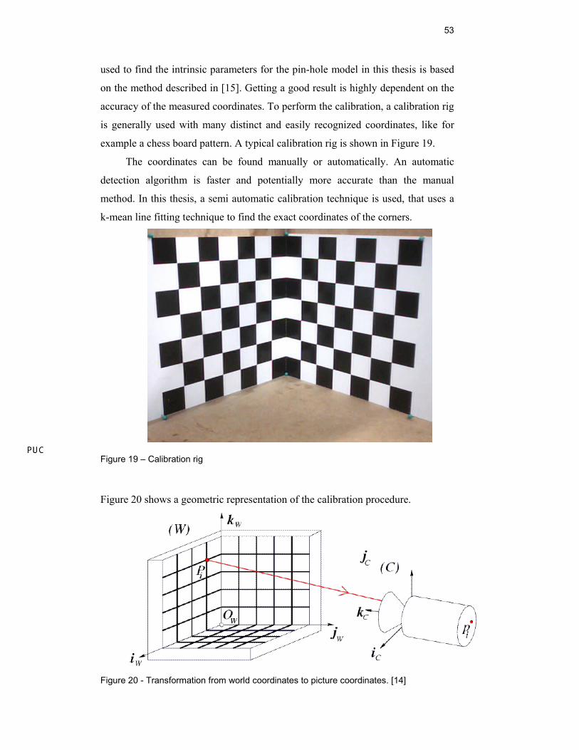
example a chess board pattern. A typical calibration rig is shown in Figure 19.
The coordinates can be found manually or automatically. An automatic
detection algorithm is faster and potentially more accurate than the manual
method. In this thesis, a semi automatic calibration technique is used, that uses a
k-mean line fitting technique to find the exact coordinates of the corners.
Figure 19 – Calibration rig
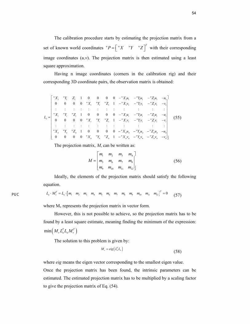
Figure 20 shows a geometric representation of the calibration procedure.
Figure 20 - Transformation from world coordinates to picture coordinates. [14]
54
The calibration procedure starts by estimating the projection matrix from a
set of known world coordinates Tw w w wP X Y Z⎡ ⎤= ⎣ ⎦ with their corresponding
image coordinates (u,v). The projection matrix is then estimated using a least
square approximation.
Having n image coordinates (corners in the calibration rig) and their
corresponding 3D coordinate pairs, the observation matrix is obtained:
1 1 1 1 1 1 1 1 1 1
1 1 1 1 1 1 1 1 1 1
1
1 0 0 0 00 0 0 0 1: : : : : : : : : : : :
1 0 0 0 00 0 0 0 1: : : : : : : : : : : :
1 0 0 0 0
w w w w w
w w w w w w
w w w w w wi i i i i i i i i i
o w w w w w wi i i i i i i i i
w w w w w wn n n n n n n n n
X Y Z X u Y u Z u uX Y Z X v Y v Z v v
X Y Z X u Y u Z u uL
X Y Z X v Y v Z v v
X Y Z X u Y u Z u u
− − − −− − − −
− − − −=
− − − −
− − − −0 0 0 0 1
nw w w w w w
n n n n n n n n n nX Y Z X v Y v Z v v
⎡ ⎤⎢ ⎥⎢ ⎥⎢ ⎥⎢ ⎥⎢ ⎥⎢ ⎥⎢ ⎥⎢ ⎥⎢ ⎥⎢ ⎥⎢ ⎥− − − −⎣ ⎦
(55)
The projection matrix, M, can be written as:
1 2 3 4
5 6 7 8
9 10 11 12
m m m mM m m m m
m m m m
⎡ ⎤⎢ ⎥= ⎢ ⎥⎢ ⎥⎣ ⎦
(56)
Ideally, the elements of the projection matrix should satisfy the following
equation.
[ ]1 2 3 4 5 6 7 8 9 10 11 12 0TTo v oL M L m m m m m m m m m m m m⋅ = ⋅ = (57)
where Mv represents the projection matrix in vector form.
However, this is not possible to achieve, so the projection matrix has to be
found by a least square estimate, meaning finding the minimum of the expression:
( )min T Tv o o vM L L M
The solution to this problem is given by:
( )Tv o oM eig L L=
(58)
where eig means the eigen vector corresponding to the smallest eigen value.
Once the projection matrix has been found, the intrinsic parameters can be
estimated. The estimated projection matrix has to be multiplied by a scaling factor
to give the projection matrix of Eq. (54).
55
( )1
2
3
x
y
z
r tM К R t К r t
r tρ
⎛ ⎞⎜ ⎟= = ⎜ ⎟⎜ ⎟⎝ ⎠
(59)
where ρ is the scaling factor, 1r , 2r and 3r are the rows of the rotation matix.
The intrinsic parameters in the calibration matrix, К, can be found with the
following procedure. The procedure is deduced in [15].
First finding the scaling factor, ρ.
[ ]9 10 11m m mερ = , 1ε = ± (60)
The first row of the rotation matrix between the camera reference frame
and the calibration rig is given by:
[ ]3 9 10 11r m m mρ= , 1ε = ± (61)
The horizontal coordinate of the image center is:
[ ]9
20 1 2 3 10
11
mu m m m m
mρ
⎡ ⎤⎢ ⎥= ⎢ ⎥⎢ ⎥⎣ ⎦
(62)
The vertical coordinate of the image center is:
[ ]9
20 5 6 7 10
11
mv m m m m
mρ
⎡ ⎤⎢ ⎥= ⎢ ⎥⎢ ⎥⎣ ⎦
(63)
The distortion angle, θ, is:
[ ] [ ]( ) [ ] [ ]( )[ ] [ ] [ ] [ ]
1 2 3 9 10 11 5 6 7 9 10 111
1 2 3 9 10 11 5 6 7 9 10 11
cosm m m m m m m m m m m m
m m m m m m m m m m m mθ −
⎛ ⎞× ⋅ ×= ⎜− ⎟
⎜ ⎟× ×⎝ ⎠
(64)
The magnification in x-direction is:
[ ] [ ]21 2 3 9 10 11 sinm m m m m mα ρ θ= × (65)
The magnification in y-direction is:
[ ] [ ]25 6 7 9 10 11 sinm m m m m mβ ρ θ= × (66)
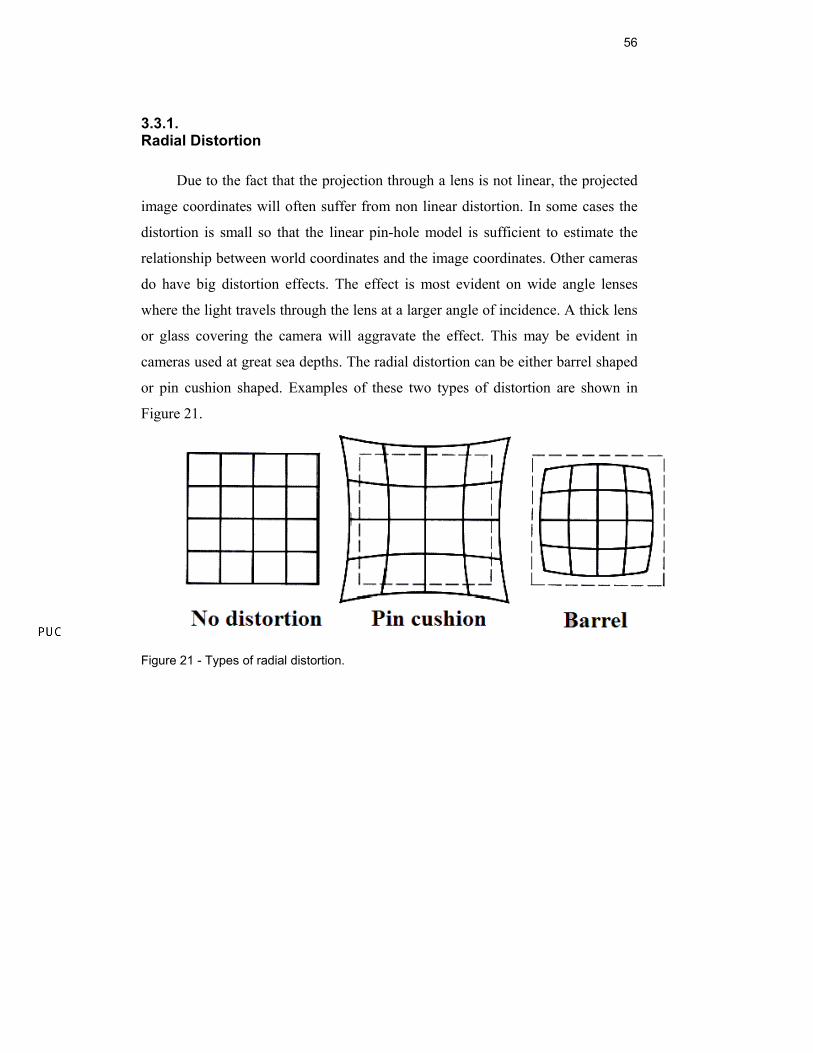
56
3.3.1. Radial Distortion
Due to the fact that the projection through a lens is not linear, the projected
image coordinates will often suffer from non linear distortion. In some cases the
distortion is small so that the linear pin-hole model is sufficient to estimate the
relationship between world coordinates and the image coordinates. Other cameras
do have big distortion effects. The effect is most evident on wide angle lenses
where the light travels through the lens at a larger angle of incidence. A thick lens
or glass covering the camera will aggravate the effect. This may be evident in
cameras used at great sea depths. The radial distortion can be either barrel shaped
or pin cushion shaped. Examples of these two types of distortion are shown in
Figure 21.
Figure 21 - Types of radial distortion.
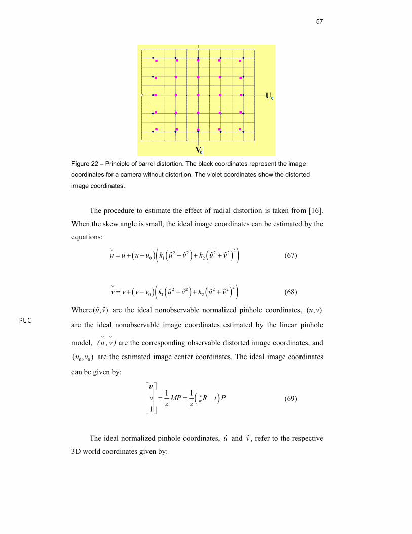
57
Figure 22 – Principle of barrel distortion. The black coordinates represent the image
coordinates for a camera without distortion. The violet coordinates show the distorted
image coordinates.
The procedure to estimate the effect of radial distortion is taken from [16].
When the skew angle is small, the ideal image coordinates can be estimated by the
equations:
( ) ( ) ( )( )22 2 2 20 1 2ˆ ˆ ˆ ˆu u u u k u v k u v
∨
= + − + + + (67)
( ) ( ) ( )( )22 2 2 20 1 2ˆ ˆ ˆ ˆv v v v k u v k u v
∨
= + − + + + (68)
Where ˆ ˆ( , )u v are the ideal nonobservable normalized pinhole coordinates, ( , )u v
are the ideal nonobservable image coordinates estimated by the linear pinhole
model, ( u∨
, v∨
) are the corresponding observable distorted image coordinates, and
0 0( , )u v are the estimated image center coordinates. The ideal image coordinates
can be given by:
( )1 1
1
cw
uv MP R t P
z z
⎡ ⎤⎢ ⎥ = =⎢ ⎥⎢ ⎥⎣ ⎦
(69)
The ideal normalized pinhole coordinates, u and v , refer to the respective
3D world coordinates given by:
58
1
ˆˆ1 1
u uv К v−
⎡ ⎤ ⎡ ⎤⎢ ⎥ ⎢ ⎥=⎢ ⎥ ⎢ ⎥⎢ ⎥ ⎢ ⎥⎣ ⎦ ⎣ ⎦
(70)
The parameters can then be estimated using alternation:
r r rD k d= (71)
Equations (66) and (67) can be given in matrix form:
( )( ) ( )( )( )( ) ( )( )
22 2 2 20 0 1
22 2 2 2 20 0
ˆ ˆ ˆ ˆ
ˆ ˆ ˆ ˆ
u u u v u u u v k u ukv v u v v v u v v v
∨
∨
⎡ ⎤ ⎡ ⎤− + − + −⎡ ⎤⎢ ⎥ ⎢ ⎥=⎢ ⎥⎢ ⎥ ⎢ ⎥⎣ ⎦− + − + −⎢ ⎥ ⎣ ⎦⎣ ⎦
(72)
Given m points and n images, the equations can be stacked together to
obtain 2mn equations. The least-square solution is given by:
( ) 11
2
T Tr r r r r
kk D D D d
k−⎡ ⎤
= =⎢ ⎥⎣ ⎦
(73)
This procedure is repeated until it converges.
3.3.2. Sophisticated calibration
This section gives a description of a more sophisticated calibration method.
Generally, if a camera is built symmetrically, the effect of radial distortion is
enough to develop an adequate mathematical model for the camera projection.
However, in some cases the radial distortion is not sufficient. This can be due to
an imprecise construction of the camera or by the fact that the camera is covered
by a casing with asymmetric characteristics. To deal with this complex distortion,
a more sophisticated calibration method needs to be applied. For this application a
calibration method presented in [17], is more appropriate. It presents a nonlinear,
iterative procedure to minimize the squared error
2 2~ ~
1i
N
i i ii
F u u v v∨ ∨
=
⎛ ⎞⎛ ⎞ ⎛ ⎞= − + −⎜ ⎟⎜ ⎟ ⎜ ⎟⎜ ⎟⎝ ⎠ ⎝ ⎠⎝ ⎠∑ (74)
59
where ( , )i iu v∨ ∨
are the estimated image coordinates using the mathematical model
and ~ ~
( , )i iu v are the observed image coordinates. The mathematical model is quite
complicated, using fifth order polynomials to estimate the distortion.
( )5 3 2 4 3 2 2 22 2 2 1 1 2 1 2 0ˆ ˆ ˆ ˆ ˆ ˆ ˆ ˆ ˆ ˆ ˆ ˆ ˆ2 3 2i u i i i i i i i i i i i i iu s f k v k u v k u v k u k u v p u p u v p v u u
∨
= + + + + + + + + + (75)
( )5 2 3 4 2 3 2 22 2 2 1 1 1 2 1 0ˆ ˆ ˆ ˆ ˆ ˆ ˆ ˆ ˆ ˆ ˆ ˆ ˆ2 2 3i i i i i i i i i i i i i iv f k v k u v k u v k u v k v p u p u v p v v v
∨
= + + + + + + + + + (76)
Having the observed image coordinates ~ ~
( , )i iu v and the estimated image
center coordinates 0 0( , )u v , the optimization is done using the Levenberg-
Marquardt algorithm. The iterative method stipulates that some camera
parameters are known. The resolution of the image sensor and its size needs to be
given. Also an initial guess of the focal length needs to be given in order to give a
good starting point for the iterations.
Using the equations (75) and (76), the image coordinates can be estimated
from a given 3D coordinate relative to the camera. However, in computer vision
the coordinates ˆ ˆ( , )i iu v are the ones of interest. It is therefore necessary to find a
way to estimate ˆ ˆ( , )i iu v from ~ ~
( , )i iu v . An implicit camera model results in:
( ) ( )( ) ( )
* * 2 4 * * 2 *21 2 3 4
* * 2 4 2 *2 * *1 2 3 4
2 2ˆ 1ˆ 2 2
i i i i i i i ii
i i i i i i i i i
u u g r g r g u v g r uuv G v v g r g r g r v g u v
⎡ ⎤+ + + + +⎡ ⎤ ⎢ ⎥=⎢ ⎥ ⎢ ⎥+ + + + +⎣ ⎦ ⎣ ⎦ (77)
where
( )2 * * 25 6 7 8 1i i i iG g r g u g v g r= + + + + (78)
~ ~
* *0 0,i ii i
u
u u v vu vs f f− −
= = (79)
~ ~
* *0 0,i ii i
u
u u v vu vs f f− −
= = (80)
60
f is the nominal focal length of the camera, su is the aspect ratio of the
image. The vector g=[ ]1 2 3 4 5 6 7 8g g g g g g g g is estimated by a least
square approximation.
Defining the observation vectors:
( )*2 2 * 4 * * 2 *2 * 4 * 2 * 2 2ˆ ˆ ˆ2 2i i ii i i i i i i i i i i i i i i iU u r u r u v r u u r u u r u v r u r⎡ ⎤= − − − − +⎣ ⎦ (81)
( )*2 2 * 4 2 *2 * * * 4 * 2 * 2 2ˆ ˆ ˆ2 2i i ii i i i i i i i i i i i i i i iV v r v r r v u v v r v u r v v r v r⎡ ⎤= − − − + −⎣ ⎦ (82)
[ ]1 1 ... ...i i N NT U V U V U V= (83)
where * * * * * *1 1 1 1 1 1 1 1ˆ ˆ ˆ ˆ ˆ ˆ... ... N N N Ne u u v v u u v v u u v v⎡ ⎤= − − − − − −⎣ ⎦ (84)
then
e Tg= (85)
( )^ 1 1Tg T T T e
− −= (86)
When the vector ^g is estimated, the ideal coordinates of the image can be
estimated using Eq.(86). However, the output of the calibration software gives the
ideal image coordinates for a nondistorted image, ( , )u v . The ideal normalized
coordinates can be estimated by Eq. (87).
^1
0^
0
00
1 0 0 1 1
iu i
i i
u fs u uv f v v
−⎡ ⎤⎢ ⎥ ⎡ ⎤ ⎡ ⎤⎢ ⎥ ⎢ ⎥ ⎢ ⎥=⎢ ⎥ ⎢ ⎥ ⎢ ⎥⎢ ⎥ ⎢ ⎥ ⎢ ⎥⎣ ⎦ ⎣ ⎦⎢ ⎥⎣ ⎦
(87)
61
3.3.3. Coordinate extraction
The coordinates of the corners of the calibration rig are most easily
extracted using an algorithm that automatically detects the edges of the image and
finds the coordinates of the corners. The image of the calibration rig offers strong
contrasts in the chess patterned surface of the rig. This means that the edges form
distinct lines that can be found using edge detection. The corners can be found
using a Harris corner detector, however this method has proven to be inaccurate
because the strength of the edges vary so that the detected corner does not fall
exactly in the crossing between two edges. This is the incentive for the proposed
extraction method using nonmaximum suppression together with k-means line
fitting to extract the coordinates. The procedure starts by manually finding the six
outer corners of the calibration rig. An initial projection matrix can be estimated
from these six coordinates. From the known geometric structure of the calibration
rig, the approximate coordinates of all the corners can be estimated using Eq. (54).
When the approximate coordinates are found, k-means line fitting is used to
estimate the actual position of the corners.
3.3.4. Nonmaximum Suppression
Nonmaximum suppression is a technique that creates a binary map
representing of the edges in an image. The image is first filtered with a Gaussian
filter to eliminate noise. The gradients of the image are then estimated in x and in
y direction using the Sobel mask. The Sobel mask used to estimate the gradient
component in x direction is given below:
1 0 12 0 21 0 1
xS−⎡ ⎤⎢ ⎥= −⎢ ⎥⎢ ⎥−⎣ ⎦
(88)
The Sobel mask used to estimate the gradient component in the y direction
is:
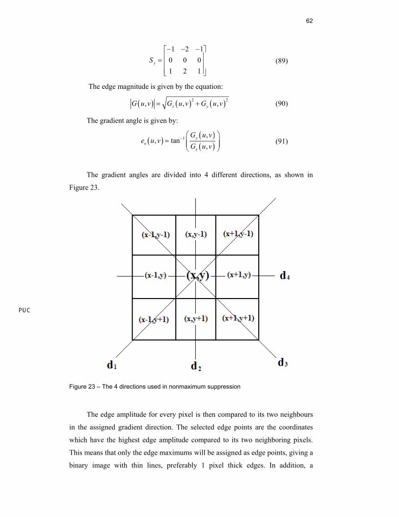
62
1 2 10 0 01 2 1
yS− − −⎡ ⎤⎢ ⎥= ⎢ ⎥⎢ ⎥⎣ ⎦
(89)
The edge magnitude is given by the equation:
( ) ( ) ( )2 2, , ,x yG u v G u v G u v= + (90)
The gradient angle is given by:
( ) ( )( )
1 ,, tan
,y
ox
G u ve u v
G u v− ⎛ ⎞
= ⎜ ⎟⎜ ⎟⎝ ⎠
(91)
The gradient angles are divided into 4 different directions, as shown in
Figure 23.
Figure 23 – The 4 directions used in nonmaximum suppression
The edge amplitude for every pixel is then compared to its two neighbours
in the assigned gradient direction. The selected edge points are the coordinates
which have the highest edge amplitude compared to its two neighboring pixels.
This means that only the edge maximums will be assigned as edge points, giving a
binary image with thin lines, preferably 1 pixel thick edges. In addition, a
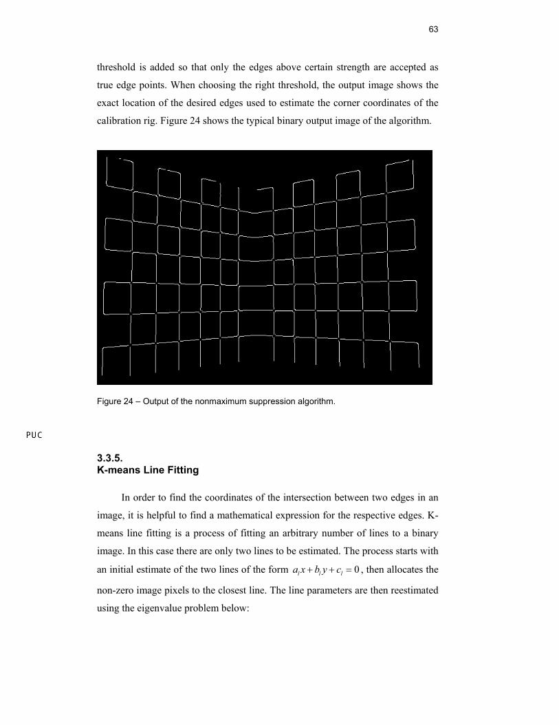
63
threshold is added so that only the edges above certain strength are accepted as
true edge points. When choosing the right threshold, the output image shows the
exact location of the desired edges used to estimate the corner coordinates of the
calibration rig. Figure 24 shows the typical binary output image of the algorithm.
Figure 24 – Output of the nonmaximum suppression algorithm.
3.3.5. K-means Line Fitting
In order to find the coordinates of the intersection between two edges in an
image, it is helpful to find a mathematical expression for the respective edges. K-
means line fitting is a process of fitting an arbitrary number of lines to a binary
image. In this case there are only two lines to be estimated. The process starts with
an initial estimate of the two lines of the form 0l l la x b y c+ + = , then allocates the
non-zero image pixels to the closest line. The line parameters are then reestimated
using the eigenvalue problem below:
64
___ __ __ ___ __ __2
______ __ __ __ __2l
l l l l l l l l ll
l ll l l l l l
x x x x y x y a ab b
x y x y y y yλ
⎡ ⎤− − ⎡ ⎤ ⎡ ⎤⎢ ⎥ ⋅ =⎢ ⎥ ⎢ ⎥⎢ ⎥ ⎣ ⎦ ⎣ ⎦⎢ ⎥− −⎣ ⎦
(92)
where ___ ___
, ,1 1
1 1, l lN N
l l i l ili il l
x x y yN N= =
= =∑ ∑
___
, ,1
1 , lN
l l l i l iil
x y x yN =
= ∑___
2 2,
1
1 pN
l l iil
x xN =
= ∑ ___
2 2,
1
1 pN
l l iil
y yN =
= ∑
This problem has two solutions. The eigen vector corresponding to the
smallest eigen value gives the best fitting line parameters. The constraint 2 2 1l la b+ = is then imposed on the solution. The line parameter lc is then found
by:
__ __
l l l l lc a x b y= − − (93)
The process is repeated until it converges, meaning that all the samples are
assigned to the same line in two consecutive iterations. The process depends on a
good initial guess in order to converge. To achieve a good result using this
method, it is required that the iterations start with initial line parameters that are
relatively close to the true values.
3.4. Feature Matching
One of the most important and challenging problems in computer vision is
finding distinct features in images that can be recognized in different scenarios. In
order to get a reliable and accurate estimate of the relative pose and translation
between two camera positions it is necessary to attain features that are both robust
and precisely positioned. In a calibration rig this is fairly easy to achieve, but on
an arbitrary object this is much more challenging. If image features are to be used
to estimate the relative position of a camera mounted at the end-effector of a
manipulator operating at great depths at sea, the feature matching has to be able to
cope with noise and be robust against changes in scale, and rotation.
65
For this task an algorithm called SIFT (“Scale Invariant Feature
Transform”) will be used. It is a fairly new algorithm developed by Lowe in 1999
[18]. In this thesis, the more recent version from 2004 [3] is used. This algorithm
satisfies all the criteria mentioned, and it is also fairly robust when it comes to
changes in luminosity. The algorithm finds a high number of interest points in the
respective images and calculates a descriptor vector from the neighboring pixels.
The Euclidian distance between the descriptor vectors is used to match the feature
points. The following section will give a more detailed description of the
algorithm.
3.4.1. Detection of Interest Points
The first stage of the SIFT algorithm is to filter the image with a Gaussian
filter to eliminate noise. The second stage is to find points that are most likely to
give robust feature vectors that can be recognized in other scenarios. The interest
points are found at the local extremes in the difference-of-Gaussian pyramid.
The Gaussian blurred image L(x,y,σ) is formed by convolving the image
I(x,y) with the Gaussian mask G(x,y,σ):
),(*),,(),,( yxIyxGyxL σσ = (94)
The function G(x,y,σ) is given by: ( )
2
22
222
1),,( σ
πσσ
yx
eyxG+−
= (95)
The algorithm becomes more efficient by subtracting the Gaussian masks
instead of subtracting the filtered images:
[ ] ),,(),,(),(*),,(),,(),,( σσσσσ yxLkyxLyxIyxGkyxGyxD −=−= (96)
1- The initial image is convolved with a Gaussian mask with a standard
deviation which increases with the scale factor k every stage. These images are
stacked in the left column.
2- For every octave the image scale is divided by an integer number, s, so
that sk1
2= , giving s+3 images in the octave so that the detection of local
maxima covers the whole octave.
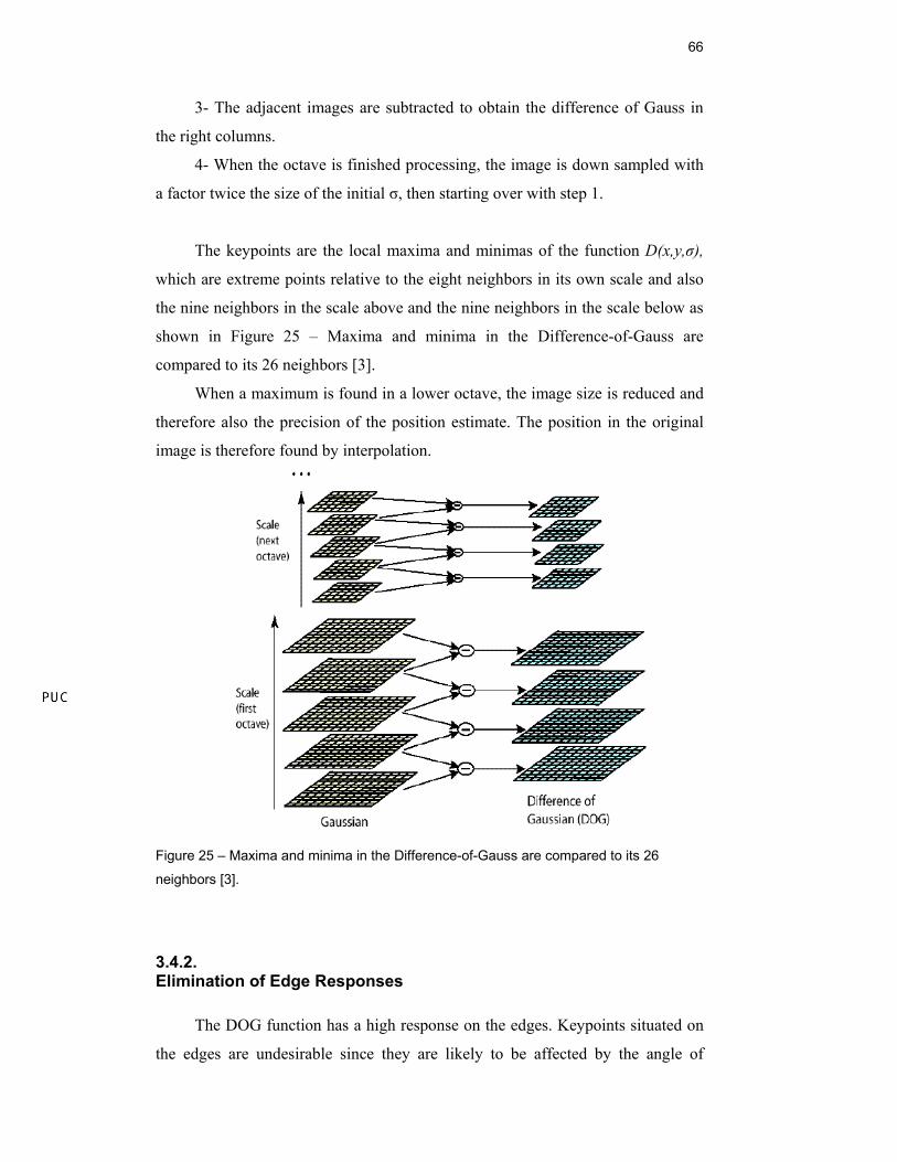
66
3- The adjacent images are subtracted to obtain the difference of Gauss in
the right columns.
4- When the octave is finished processing, the image is down sampled with
a factor twice the size of the initial σ, then starting over with step 1.
The keypoints are the local maxima and minimas of the function D(x,y,σ),
which are extreme points relative to the eight neighbors in its own scale and also
the nine neighbors in the scale above and the nine neighbors in the scale below as
shown in Figure 25 – Maxima and minima in the Difference-of-Gauss are
compared to its 26 neighbors [3].
When a maximum is found in a lower octave, the image size is reduced and
therefore also the precision of the position estimate. The position in the original
image is therefore found by interpolation.
Figure 25 – Maxima and minima in the Difference-of-Gauss are compared to its 26
neighbors [3].
3.4.2. Elimination of Edge Responses
The DOG function has a high response on the edges. Keypoints situated on
the edges are undesirable since they are likely to be affected by the angle of
67
incidence of the light. The curvature of an edge is strong in the gradient direction
but weak in the perpendicular direction. The Hessian matrix is therefore used to
eliminate the keypoints that are found on or close to an edge maximum. The
Hessian matrix of the function D is given by the equation:
⎥⎦
⎤⎢⎣
⎡=
YYXY
XYXX
DDDD
H (97)
The largest eigenvalue of H is denoted by λ1 be and the smallest eigenvalue
is denoted by λ2. The ratio between the eigenvalues can be found by the trace and
determinant of H.
1 22
1 2
( )
( )XX YY
XX YY XY
Tr H D D
Det H D D D
λ λ
λ λ
= + = +
= − = (98)
Defining rλ as the ratio between λ1 and λ2 giving λ1= rλ λ2, then:
( ) ( )2 2 221 2 2 2
21 2 2
( 1)( )( )
r rTr HDet H r r
λ λ
λ
λ λ λ λλ λ λ+ + +
= = = (99)
rλ denotes the principal curvature. The principal curvature has to be above
a certain value to ensure that the keypoint is not located on an edge. Elimination
of the edge points is done by removing the keypoints that satisfy the following
equation: 22 ( 1)( )
( )rTr H
Det H rλ
λ
+< (100)
In all the experiments in this thesis, a threshold of rλ=10 is used.
3.4.3. Accurate keypoint localization
The next step is to perform a detailed fit of the keypoint to its nearby data.
The characteristics of the DOG function are estimated using a Taylor expansion
around the keypoint location show in the equation below: 2
2
1( )2
TTD DD x D x x x
x x∂ ∂
= + +∂ ∂
(101)
68
where D and its derivatives are evaluated at he same point and x=(x,y,σ) T is the
offset from this point. The localization of the extremum, x , is determined by
setting the derivative of the Taylor expansion to zero, giving
xD
xDx
∂∂
∂∂
−=−
2
12
ˆ (102)
The exact location of the extremum is used to determine the exact position
of the keypoint, giving it a higher precision than one pixel. The peak value of,
D( x ), is used to eliminate keypoints with low contrast since they are more easily
affected by noise. The maximum value can be estimated by substituting Eq.(102)
into Eq.(101) giving:
xx
DDxDT
ˆ21)ˆ(
∂∂
+= (103)
In the experiments in this thesis all keypoints with a contrast lower than
0.03 are rejected.
3.4.4. Assigning Orientation
To obtain a feature descriptor invariant to camera rotation, each keypoint is
assigned an orientation estimated from local edge tangents in the image. For all
the pixels in the image, L(x,y), the edge magnitude m(x,y) and edge orientation
θ(x,y) are calculated by the following equations:
( ) ( )2 2( , ) ( 1, ) ( 1, ) ( , 1) ( , 1)m x y L x y L x y L x y L x y= + − − + + − − (104)
( )( )
1 ( , 1) ( , 1)( , ) tan
( 1, ) ( 1, )L x y L x y
x yL x y L x y
θ − ⎛ ⎞+ − −= ⎜ ⎟⎜ ⎟+ − −⎝ ⎠
(105)
In the surrounding, region there will be a prevailing orientation that is found
by forming a histogram of 36 regions, shown in Figure 26. The prevailing
orientation in the histogram will be the orientation of the keypoint. Finally, the
exact orientation is found by interpolating a parabola to find the center of the
group.
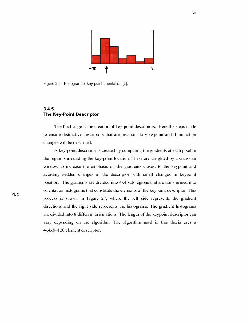
69
Figure 26 – Histogram of key-point orientation [3].
3.4.5. The Key-Point Descriptor
The final stage is the creation of key-point descriptors. Here the steps made
to ensure distinctive descriptors that are invariant to viewpoint and illumination
changes will be described.
A key-point descriptor is created by computing the gradients at each pixel in
the region surrounding the key-point location. These are weighted by a Gaussian
window to increase the emphasis on the gradients closest to the keypoint and
avoiding sudden changes in the descriptor with small changes in keypoint
position. The gradients are divided into 4x4 sub regions that are transformed into
orientation histograms that constitute the elements of the keypoint descriptor. This
process is shown in Figure 27, where the left side represents the gradient
directions and the right side represents the histograms. The gradient histograms
are divided into 8 different orientations. The length of the keypoint descriptor can
vary depending on the algorithm. The algorithm used in this thesis uses a
4x4x8=120 element descriptor.
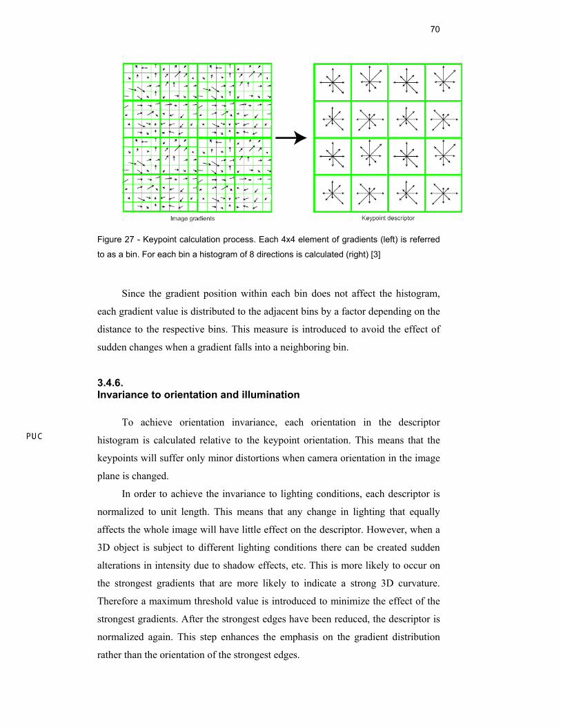
70
Figure 27 - Keypoint calculation process. Each 4x4 element of gradients (left) is referred
to as a bin. For each bin a histogram of 8 directions is calculated (right) [3]
Since the gradient position within each bin does not affect the histogram,
each gradient value is distributed to the adjacent bins by a factor depending on the
distance to the respective bins. This measure is introduced to avoid the effect of
sudden changes when a gradient falls into a neighboring bin.
3.4.6. Invariance to orientation and illumination
To achieve orientation invariance, each orientation in the descriptor
histogram is calculated relative to the keypoint orientation. This means that the
keypoints will suffer only minor distortions when camera orientation in the image
plane is changed.
In order to achieve the invariance to lighting conditions, each descriptor is
normalized to unit length. This means that any change in lighting that equally
affects the whole image will have little effect on the descriptor. However, when a
3D object is subject to different lighting conditions there can be created sudden
alterations in intensity due to shadow effects, etc. This is more likely to occur on
the strongest gradients that are more likely to indicate a strong 3D curvature.
Therefore a maximum threshold value is introduced to minimize the effect of the
strongest gradients. After the strongest edges have been reduced, the descriptor is
normalized again. This step enhances the emphasis on the gradient distribution
rather than the orientation of the strongest edges.
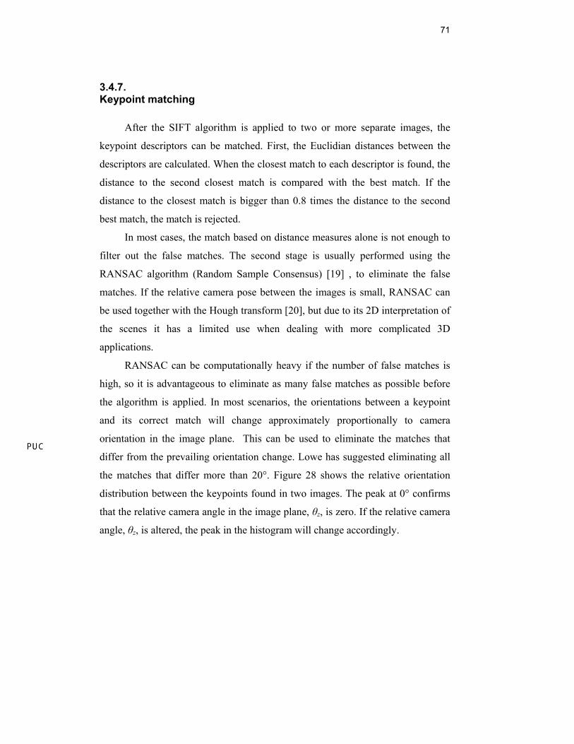
71
3.4.7. Keypoint matching
After the SIFT algorithm is applied to two or more separate images, the
keypoint descriptors can be matched. First, the Euclidian distances between the
descriptors are calculated. When the closest match to each descriptor is found, the
distance to the second closest match is compared with the best match. If the
distance to the closest match is bigger than 0.8 times the distance to the second
best match, the match is rejected.
In most cases, the match based on distance measures alone is not enough to
filter out the false matches. The second stage is usually performed using the
RANSAC algorithm (Random Sample Consensus) [19] , to eliminate the false
matches. If the relative camera pose between the images is small, RANSAC can
be used together with the Hough transform [20], but due to its 2D interpretation of
the scenes it has a limited use when dealing with more complicated 3D
applications.
RANSAC can be computationally heavy if the number of false matches is
high, so it is advantageous to eliminate as many false matches as possible before
the algorithm is applied. In most scenarios, the orientations between a keypoint
and its correct match will change approximately proportionally to camera
orientation in the image plane. This can be used to eliminate the matches that
differ from the prevailing orientation change. Lowe has suggested eliminating all
the matches that differ more than 20°. Figure 28 shows the relative orientation
distribution between the keypoints found in two images. The peak at 0° confirms
that the relative camera angle in the image plane, θz, is zero. If the relative camera
angle, θz, is altered, the peak in the histogram will change accordingly.
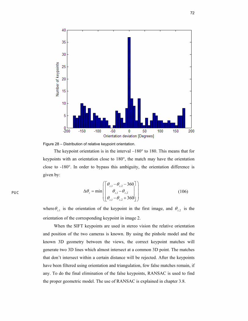
72
Figure 28 – Distribution of relative keypoint orientation.
The keypoint orientation is in the interval –180° to 180. This means that for
keypoints with an orientation close to 180°, the match may have the orientation
close to -180°. In order to bypass this ambiguity, the orientation difference is
given by:
,1 ,2
,1 ,2
,1 ,2
360min
360
z z
z z z
z z
θ θθ θ θ
θ θ
⎛ ⎞⎡ ⎤− −⎜ ⎟⎢ ⎥∆ = −⎜ ⎟⎢ ⎥⎜ ⎟⎢ ⎥− +⎣ ⎦⎝ ⎠
(106)
where ,1zθ is the orientation of the keypoint in the first image, and ,2zθ is the
orientation of the corresponding keypoint in image 2.
When the SIFT keypoints are used in stereo vision the relative orientation
and position of the two cameras is known. By using the pinhole model and the
known 3D geometry between the views, the correct keypoint matches will
generate two 3D lines which almost intersect at a common 3D point. The matches
that don’t intersect within a certain distance will be rejected. After the keypoints
have been filtered using orientation and triangulation, few false matches remain, if
any. To do the final elimination of the false keypoints, RANSAC is used to find
the proper geometric model. The use of RANSAC is explained in chapter 3.8.
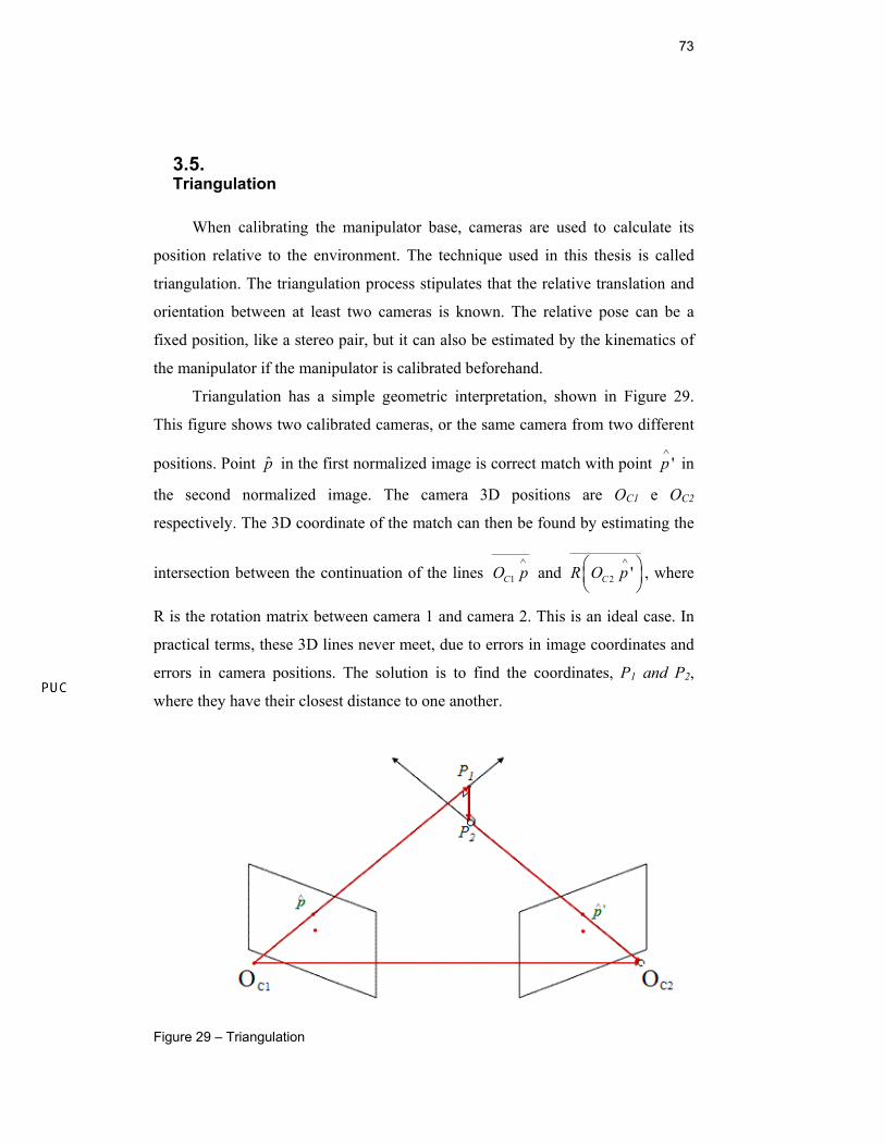
73
3.5. Triangulation
When calibrating the manipulator base, cameras are used to calculate its
position relative to the environment. The technique used in this thesis is called
triangulation. The triangulation process stipulates that the relative translation and
orientation between at least two cameras is known. The relative pose can be a
fixed position, like a stereo pair, but it can also be estimated by the kinematics of
the manipulator if the manipulator is calibrated beforehand.
Triangulation has a simple geometric interpretation, shown in Figure 29.
This figure shows two calibrated cameras, or the same camera from two different
positions. Point p in the first normalized image is correct match with point 'p∧
in
the second normalized image. The camera 3D positions are OC1 e OC2
respectively. The 3D coordinate of the match can then be found by estimating the
intersection between the continuation of the lines ________
1CO p∧
and _______________
2 'CR O p∧⎛ ⎞
⎜ ⎟⎝ ⎠
, where
R is the rotation matrix between camera 1 and camera 2. This is an ideal case. In
practical terms, these 3D lines never meet, due to errors in image coordinates and
errors in camera positions. The solution is to find the coordinates, P1 and P2,
where they have their closest distance to one another.
Figure 29 – Triangulation
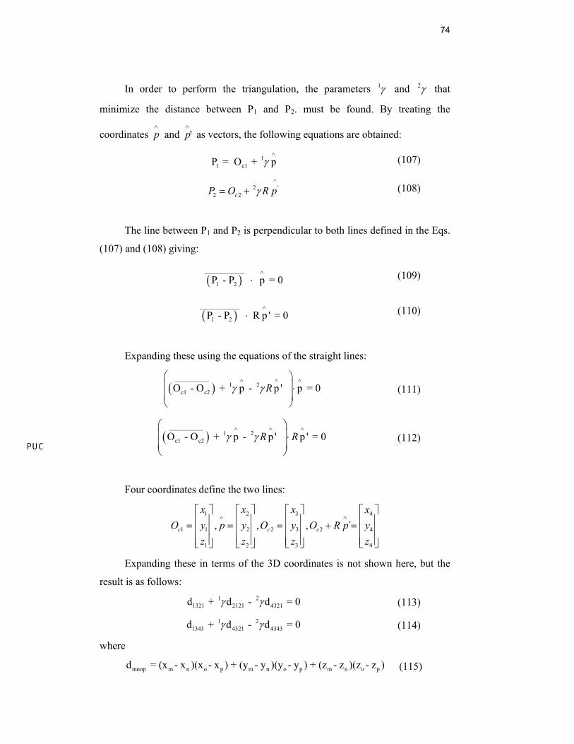
74
In order to perform the triangulation, the parameters 1γ and 2γ that
minimize the distance between P1 and P2. must be found. By treating the
coordinates p∧
and 'p∧
as vectors, the following equations are obtained:
11 c1P = O + pγ
∧
(107)
^2 '
2 2cP O R pγ= + (108)
The line between P1 and P2 is perpendicular to both lines defined in the Eqs.
(107) and (108) giving:
( )_____________
1 2P - P p = 0∧
⋅ (109)
( )_____________
1 2P - P R p ' = 0∧
⋅ (110)
Expanding these using the equations of the straight lines:
( )___________
1 2c1 c2O - O + p - p ' p = 0 Rγ γ
∧ ∧ ∧⎛ ⎞⎜ ⎟ ⋅⎜ ⎟⎝ ⎠
(111)
( )___________
1 2c1 c2O - O + p - p ' p ' = 0 R Rγ γ
∧ ∧ ∧⎛ ⎞⎜ ⎟ ⋅⎜ ⎟⎝ ⎠
(112)
Four coordinates define the two lines:
1 2 3 4
1 1 2 2 3 2 4
1 2 3 4
, , , ´c c c
x x x xO y p y O y O R p y
z z z z
∧ ∧⎡ ⎤ ⎡ ⎤ ⎡ ⎤ ⎡ ⎤⎢ ⎥ ⎢ ⎥ ⎢ ⎥ ⎢ ⎥= = = + =⎢ ⎥ ⎢ ⎥ ⎢ ⎥ ⎢ ⎥⎢ ⎥ ⎢ ⎥ ⎢ ⎥ ⎢ ⎥⎣ ⎦ ⎣ ⎦ ⎣ ⎦ ⎣ ⎦
Expanding these in terms of the 3D coordinates is not shown here, but the
result is as follows: 1 2
1321 2121 4321d + d - d = 0γ γ (113)
1 21343 4321 4343d + d - d = 0γ γ (114)
where
mnop m n o p m n o p m n o pd = (x - x )(x - x ) + (y - y )(y - y ) + (z - z )(z - z ) (115)
75
Finally, solving for 1γ gives:
1 1343 4321 1321 4343
2121 4343 4321 4321
d d - d d = d d - d ·d
γ (116)
Back substituting gives 2γ
12 1343 4321
4343
d + d = d
γγ (117)
By using Eqs. (107) and (108) the coordinates of the closest point can be
estimated for both lines. This is handy when it comes to eliminating false keypoint
matches.
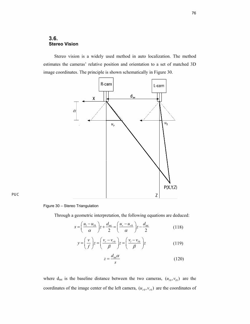
76
3.6. Stereo Vision
Stereo vision is a widely used method in auto localization. The method
estimates the cameras’ relative position and orientation to a set of matched 3D
image coordinates. The principle is shown schematically in Figure 30.
Figure 30 – Stereo Triangulation
Through a geometric interpretation, the following equations are deduced:
0 int 0 int
2 2l l r ru u d u u dx z zα α− −⎛ ⎞ ⎛ ⎞= + = −⎜ ⎟ ⎜ ⎟
⎝ ⎠ ⎝ ⎠ (118)
0 0r r l lv v v vvy z z zf β β
⎛ ⎞ ⎛ − ⎞ ⎛ − ⎞= = =⎜ ⎟ ⎜ ⎟ ⎜ ⎟
⎝ ⎠ ⎝ ⎠⎝ ⎠ (119)
intdzsα
= (120)
where dint is the baseline distance between the two cameras, 0 0( , )l lu v are the
coordinates of the image center of the left camera, 0 0( , )r ru v are the coordinates of
77
the image center of the right camera, ( , )l lu v are the image coordinates of the left
camera corresponding to the point P(x,y,z), ( , )r ru v are the image coordinates of
the right camera corresponding to the point P(x,y z), and 0 0( )r r l ls u u u u= − − −
represents the x coordinate change [pixels] between the left and the right image.
To get an idea of the accuracy of the estimated coordinates, the sensitivity
relative to a change in image coordinates is estimated. The position error of the
point P(x,y z) is given by the following equations:
202
int
u ux z sdα
⎛ ⎞−∆ = − ∆⎜ ⎟
⎝ ⎠ (121)
202
int
v vy z sdβ
⎛ ⎞−∆ = − ∆⎜ ⎟
⎝ ⎠ (122)
2
int
1z z sdα
⎛ ⎞∆ = − ∆⎜ ⎟
⎝ ⎠ (123)
where x∆ is the error in x direction, y∆ is the error in y direction, z∆ is the error
in z direction, α is the magnification factor in x direction, β is the magnification
factor in y direction and s∆ is the is the error of s. The image coordinates v, v0, u
and u0 are the image coordinates of the chosen reference camera. It can be either
the left or the right camera.
It is obvious from these equations that the accuracy of the coordinates is
highly dependent on the resolution of the camera and the intraocular distance
between the two stereo cameras. Having a stereo pair attached at the end effector
restricts the feasible size of the camera system and thus the possible intraocular
distance. This is the incentive for the idea presented in Chapter 3.9, which uses the
manipulator kinematics to place the camera in different positions, allowing an
arbitrary intraocular distance.
The calibration of the manipulator structure increases the repeatability and
absolute precision of the manipulator. This makes it possible to move the camera
to any desired position relative to the object of interest and calculate the relative
orientation and translation. The manipulator does not offer the same intraocular
distance accuracy as a stereo pair camera, but the high versatility makes it a good
alternative when the range to the object of interest is high.
78
3.7. Manipulator Base Calibration
In order to use stereo vision to estimate the relative movement of a camera,
two sets of 3D coordinates has to be created by triangulation. The first set, 1 p , is
generated from known camera positions relative to the environment. To estimate
the relative movement of the camera when found in another position, a second
corresponding 3D coordinate set, 2 p , has to be created. The sets 1 p and 2 p give
the position of the same coordinates, but with different reference frames.
Estimating the translation and rotation of the reference frames will give the
relative movement of the camera.
Estimation of the reference frame can be done in several ways. The first
method investigated here was to generate the 4 x 4 homogeneous transformation
matrix using a minimum least square technique. However, this technique was very
sensitive to noise and did not give an accurate result compared to other methods.
The second method that was implemented and tested was generation of the
relative rotation matrix, R, by using a least square technique suggested in [21].
Having two sets of 3D coordinates 1 p and 2 p each containing m samples
representing the same coordinates given two different reference frames. The
relationship between the i-th coordinate sets is given by: 2 1
i iR p t p⋅ + = (124)
Where R is the rotation matrix between the coordinates and t is the translation
vector relative to the reference frame of 1 p . The rotation matrix can be calculated
by using quaternions or by the least square estimate suggested in [21].
When the rotation matrix, R, is calculated, the translation can be found by:
( )1 21 m
i ii
t p R pm
= − ⋅∑ (125)
where m is the number of samples in each set of coordinates
79
The translation between the cameras is then estimated using Eq.(125). This
method has shown a better result than the direct estimation of the homogeneous
matrix.
In an attempt improve the position estimate even further, another method to
estimate the rotation matrix has been tested. The method estimates the rotation
matrix using quaternions. The relative position of the cameras is then estimated
using Eq.(125). This method has proven to be more accurate than the least square
method when there are outliers in the coordinate sets. The quaterninon techniques
are deduced in Chapter 3.7.2.
3.7.1. Quaternion Algebra
A quaternion is an extension of the concept of complex numbers [22]. A
quaternion can be written in the form:
0 1 2 3q a a i a j a k= + + + (126)
where i, j and k are complex quaternion units. The unit vectors are orthogonal 3D
vectors and , ,i j k j k i k i j× = × = × =
The quaternion can be written in the simplified form:
0 ,TTq a a⎡ ⎤= ⎣ ⎦ (127)
The Hamilton conjugate is defined by:
*0 ,
TTq a a⎡ ⎤= −⎣ ⎦ (128)
When working with quaternions it is necessary to know the basic rules of
different operations. Define the two quaternions a= 0,TTa a⎡ ⎤⎣ ⎦ and b= 0 ,
TTb b⎡ ⎤⎣ ⎦ .
Addition and subtraction of the two quaternions follow the following rule.
a ± b 0 0 ,TT Ta b a b⎡ ⎤= ± ±⎣ ⎦ (129)
Multiplication of two quaternions follow the following rule:
a ◦ b ( )0 0 0 0,TTa b a b a b b a a b⎡ ⎤= − ⋅ + + ×⎣ ⎦ (130)
The norm of a quaternion is defined by:
( ) 2Ta a a= aN = (131)
The inverse of a nonzero quaternion is given by:
80
( )*
-1 aaaN
= (132)
When dealing with pure rotations, the quaternions are unit quaternions
with norm=1. This means that for a quaternion [ ]0 1 2 3Tq q q q q= ,
1 *q q− = and it can be written in the following way:
cos sin k2 2
q θ θ⎛ ⎞ ⎛ ⎞= +⎜ ⎟ ⎜ ⎟⎝ ⎠ ⎝ ⎠
(133)
If the 3D coordinate y can be expressed as a pure rotation of 3D
coordinate x, the corresponding equation is:
y R x= ⋅ (134)
The same equation can be expressed in the following way using
quaternions: *y q x q= (135)
The rotation matrix (R) in Eq.(134) can be estimated from the
corresponding quaternion using the following equation:
( ) ( )( ) ( )( ) ( )
2 2 2 20 1 2 3 1 2 0 3 1 3 0 2
2 2 2 21 2 0 3 0 1 2 3 2 3 0 1
2 2 2 21 3 0 2 2 3 0 1 0 1 2 3
2 22 22 2
q q q q q q q q q q q qR q q q q q q q q q q q q
q q q q q q q q q q q q
⎡ ⎤+ − − − +⎢ ⎥= + − + − −⎢ ⎥⎢ ⎥− + − − +⎣ ⎦
(136)
3.7.2. Estimation of the Rotation Matrix Using Quaternions
Consider a 3D coordinate 1 p . Written in another reference frame the same
coordinates take the form 2 p . Transformation between the coordinates is given by
the following equation: 2 1R p p t⋅ = − (137)
When using quaternions, the following equation is used:
2 2 *R p q p q⋅ = (138)
Substituting Eq.(138) into Eq.(137) gives
( )2 1 0q p p t q− − = (139)
Expanding Eq.(139) gives:
81
( ) ( ) ( ) ( )( )2 2 2 1 1 1, ,q p q p p q q p t q p t p t⋅ ⋅ − × = ⋅ − − × − (140)
Because the scalar part , ( )2 1 0q p p t q− − = , Eq.(140) is equal to:
( )( ) ( )( )2 1 2 1p p t q q p p t+ − × = − − (141)
For the matrix R to be a rotation matrix, cos sin2 2q qq
θ θ⎛ ⎞ ⎛ ⎞= +⎜ ⎟ ⎜ ⎟
⎝ ⎠ ⎝ ⎠k , where k
is the rotation axis and θ is the rotation angle of R respectively. Substituting this
into Eq.(141) gives:
( )1 2 2 1tan2
kq p t p p p tθ⎛ ⎞
− + × = − +⎜ ⎟⎝ ⎠
(142)
Defining the scew matrix ( )0
00
z y
z x
y x
v vQ v v v
v v
⎡ ⎤−⎢ ⎥= −⎢ ⎥⎢ ⎥−⎣ ⎦
, which has the
following property for the vector x y zv v v v⎡ ⎤= ⎣ ⎦ .
( ) q qQ v x v x⋅ = × (143)
Equation (142) can then be written as:
( ) ( )2 1 2 1q qQ p p x Q t x t p p+ − − = − (144)
where:
tan2q
qxθ⎛ ⎞
= ⎜ ⎟⎝ ⎠
k (145)
which is the Rodrigues parameter and
( )q qy Q t x t= − − (146)
Equation (144) can then be written as:
( )1 2 2 1q qQ p p x y p p− + = − (147)
Assuming that there are m available coordinate pairs, to estimate the
rotation quaternion from these m measurements the variable yq can be eliminated
by substituting 2 2i i i+1= p pζ − and 1 1
i i i+1= p pρ − , giving the equation:
( )i i q i iQ xζ ρ ζ ρ+ = + (148)
82
which holds for all i=1:m measurements. This equation can be solved with a
minimum of three measured coordinate pairs, giving the exact solution by solving
the equation:
q q qA x b⋅ = (149)
where
( )( )
1 1
2 2q
QA
Qζ ρζ ρ
+⎡ ⎤= ⎢ ⎥+⎣ ⎦
(150)
and
1 1
2 2qb
ζ ρζ ρ
−⎡ ⎤= ⎢ ⎥−⎣ ⎦
(151)
Having more than three measurements the equation can be solved by means
of the pseudo inverse matrix:
( ) 1Tq q q q q x = A TA A b
− (152)
where
( )
( )( )
1 1
q
1 1
.
.
.
m m
m m
Q
A
ζ ρ
ζ ρζ ρ− −
+⎡ ⎤⎢ ⎥⎢ ⎥⎢ ⎥
= ⎢ ⎥⎢ ⎥⎢ ⎥+⎢ ⎥
+⎢ ⎥⎣ ⎦
(153)
and
1 1
1 1
.
.
.q
m m
m m
b
ζ ρ
ζ ρζ ρ− −
−⎡ ⎤⎢ ⎥⎢ ⎥⎢ ⎥
= ⎢ ⎥⎢ ⎥⎢ ⎥−⎢ ⎥
−⎢ ⎥⎣ ⎦
(154)
After solving for qx , the quaternion q can be estimated. The vector k from
Eq.(133) is found by:
q
q
xk=
x (155)
The angle θq from Eq.(133) is found by:
83
( )( )
q-1max x
2 tanmaxqθ
⎛ ⎞⎜ ⎟⎜ ⎟⎝ ⎠
=k
(156)
The rotation quaternion is then found by Eq.(133) and the rotation matrix is
given by Eq.(136).
3.8. Elimination of Keypoint Matches using RANSAC
If the correct orientation and translation between two views have been
found, the samples in the coordinate sets should ideally satisfy Eq.(124).
However, after filtering the keypoint matches by their orientation angles and their
point of coincidence, there might still remain some false matches in the sets. To
eliminate these remaining outliers, RANSAC is used together with Eq.(124) to
find which samples satisfy the 3D model. The rotation matrix, R, can be estimated
using three corresponding samples from the sets 1 p and 2 p . The syntax of the
algorithm is as follows:
a) 2 1i iR p t p⋅ + =
b) Randomly pick 3 corresponding samples from the sets 1 p and 2 p forming 1 *p and 2 *p
c) Estimate the relative rotation matrix, R, between the samples using 1 *p and 2 *p . This can either be done by using the quaternion technique deduced in
section 3.7.2 or by the least mean square technique presented in [21].
d) Estimate the mean of 1 *p and 2 *p denoted by ~
1 *p and ~
2 *p
e) Generate a new set of translated coordinates:
~
1 1 1 *t i ip p p= − (157)
~2 2 2 *t i ip p p= −
(158)
If the correct rotation matrix is estimated, the samples should satisfy the
following equation:
2 1t i t iR p p= (159)
84
However, due to uncertainties in the estimated coordinates, a certain error
has to be tolerated. The samples that satisfy the following equation are accepted
by the model.
2 1,t i t i r i rR p p d d− = < (160)
After a number of iterations the model that includes the highest number of
samples is used to generate the final rotation matrix. The position is then
estimated using Eq.(124).
After RANSAC is applied to the data sets, any outlier with a detrimental
effect to the model is eliminated. The remaining samples all fit the model, some
better than others. To further increase the accuracy of the measured position, a last
filtering can be done. The samples that are close to the center of the cluster of
samples are less important when it comes to estimating the relative rotation
matrix. They might even have a negative effect on the accuracy. Defining the
error ratio by the following equation:
~1 1
,,
R Ri
e ir i
p pr
d
−= (161)
where dr,i is the Euclidian distance error from Eq.(160). 1R ip are the coordinates of
1 p after RANSAC has eliminated the outliers, and ~
1R p is the center of the
coordinate set 1R p .
The sample with the highest value of re,i is then eliminated and the rotation
matrix is reestimated. The process is then repeated until all the samples in the sets
have an error ratio less than a chosen limit, limr .
This final step has proven to improve the estimated position accuracy. This
can be seen in the experiments in Chapter 5.
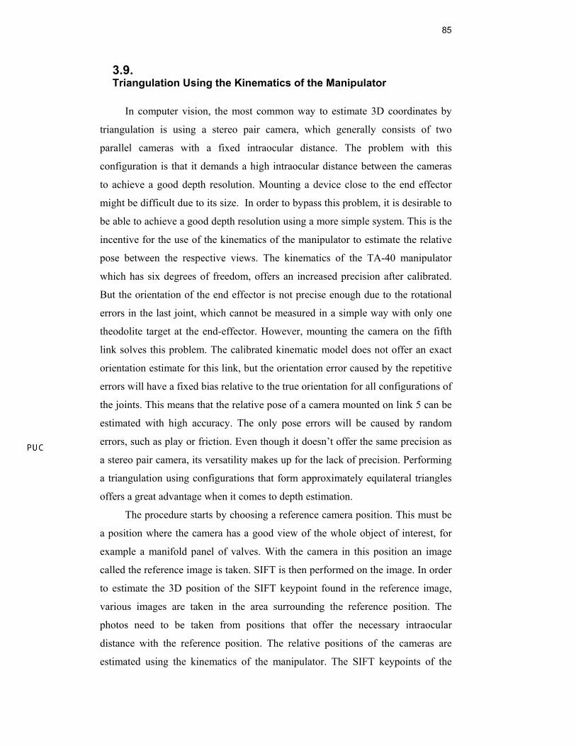
85
3.9. Triangulation Using the Kinematics of the Manipulator
In computer vision, the most common way to estimate 3D coordinates by
triangulation is using a stereo pair camera, which generally consists of two
parallel cameras with a fixed intraocular distance. The problem with this
configuration is that it demands a high intraocular distance between the cameras
to achieve a good depth resolution. Mounting a device close to the end effector
might be difficult due to its size. In order to bypass this problem, it is desirable to
be able to achieve a good depth resolution using a more simple system. This is the
incentive for the use of the kinematics of the manipulator to estimate the relative
pose between the respective views. The kinematics of the TA-40 manipulator
which has six degrees of freedom, offers an increased precision after calibrated.
But the orientation of the end effector is not precise enough due to the rotational
errors in the last joint, which cannot be measured in a simple way with only one
theodolite target at the end-effector. However, mounting the camera on the fifth
link solves this problem. The calibrated kinematic model does not offer an exact
orientation estimate for this link, but the orientation error caused by the repetitive
errors will have a fixed bias relative to the true orientation for all configurations of
the joints. This means that the relative pose of a camera mounted on link 5 can be
estimated with high accuracy. The only pose errors will be caused by random
errors, such as play or friction. Even though it doesn’t offer the same precision as
a stereo pair camera, its versatility makes up for the lack of precision. Performing
a triangulation using configurations that form approximately equilateral triangles
offers a great advantage when it comes to depth estimation.
The procedure starts by choosing a reference camera position. This must be
a position where the camera has a good view of the whole object of interest, for
example a manifold panel of valves. With the camera in this position an image
called the reference image is taken. SIFT is then performed on the image. In order
to estimate the 3D position of the SIFT keypoint found in the reference image,
various images are taken in the area surrounding the reference position. The
photos need to be taken from positions that offer the necessary intraocular
distance with the reference position. The relative positions of the cameras are
estimated using the kinematics of the manipulator. The SIFT keypoints of the
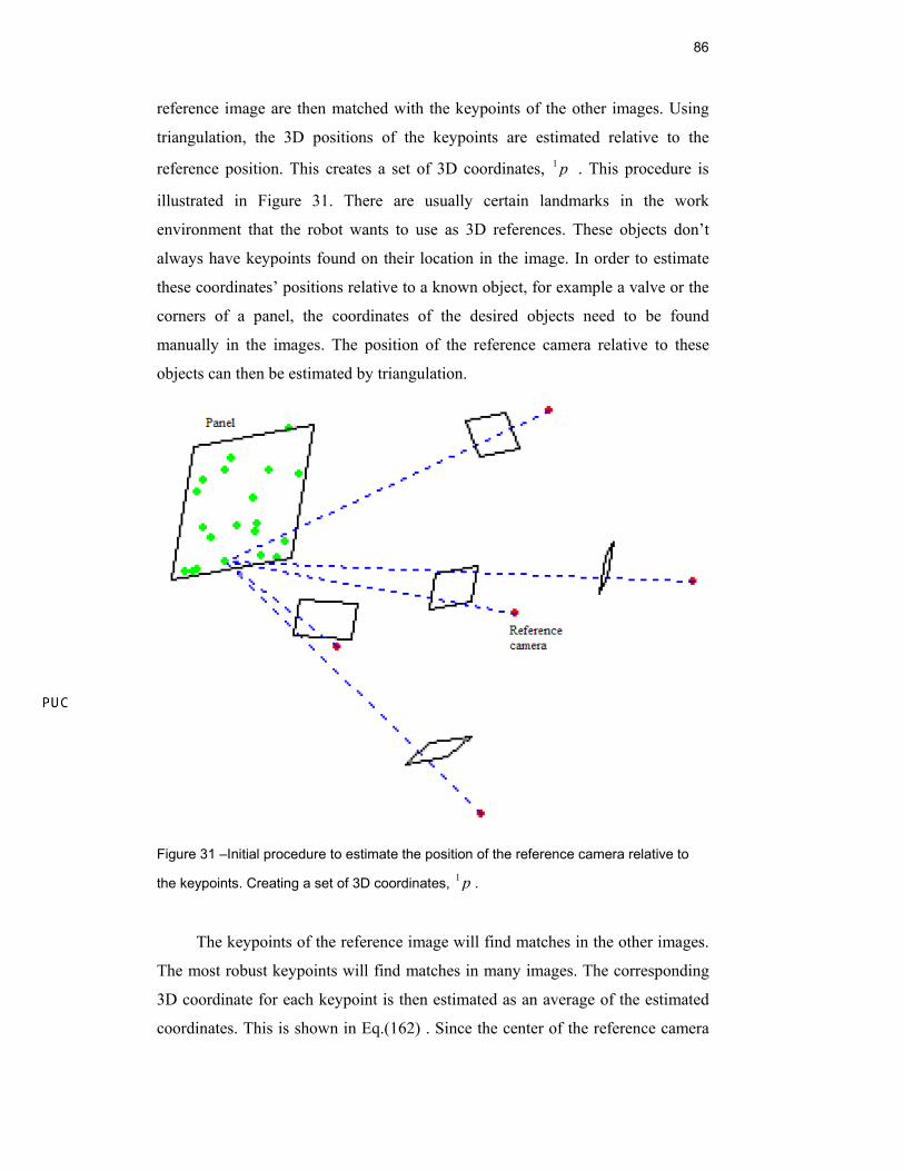
86
reference image are then matched with the keypoints of the other images. Using
triangulation, the 3D positions of the keypoints are estimated relative to the
reference position. This creates a set of 3D coordinates, 1 p . This procedure is
illustrated in Figure 31. There are usually certain landmarks in the work
environment that the robot wants to use as 3D references. These objects don’t
always have keypoints found on their location in the image. In order to estimate
these coordinates’ positions relative to a known object, for example a valve or the
corners of a panel, the coordinates of the desired objects need to be found
manually in the images. The position of the reference camera relative to these
objects can then be estimated by triangulation.
Figure 31 –Initial procedure to estimate the position of the reference camera relative to
the keypoints. Creating a set of 3D coordinates, 1 p .
The keypoints of the reference image will find matches in the other images.
The most robust keypoints will find matches in many images. The corresponding
3D coordinate for each keypoint is then estimated as an average of the estimated
coordinates. This is shown in Eq.(162) . Since the center of the reference camera
87
defines the origin of the reference frame, the equation does not need to include a
rotation matrix.
1
1 1, ,
11
1 cN
i i j i jjc
p pN
γ∧
=
⎛ ⎞= ⎜ ⎟⎝ ⎠
∑ (162)
where 1cN is the number of images where each keypoint is found, ip∧
is the
normalized image coordinate for the respective keypoint, and 1,i jγ is the
multiplication factor deduced on Chapter 3.5 that denotes where the line through
the normalized coordinate ip∧
intersects with the line through ,i jp∧
of the j-th
image. This gives:
( )1
1 1 1, ,
11
1 cN
i i j i jjc
p К pN
γ −
=
= ∑ (163)
To avoid that any false keypoint matches will ruin the estimated coordinate,
the Euclidian distance between all the corresponding coordinates are estimated.
The coordinates that don’t have a neighbour within a distance dn are not used in
the estimate. After these coordinates have been eliminate, 1cN matches remain to
estimate the final coordinate 1ip .
The coordinates can also be estimated in an alternative way, by estimating
where the line through ,i jp∧
has its closest point to ip∧
:
( )1 * 2 1, ,
11
1i j
nT
j i j i jjc
p t R К pN
γ −
=
= + ⋅ ⋅∑ (164)
where tj is the position of the j-th camera relative to the reference camera, Rj is the
rotation matrix between the chosen reference camera and the j-th camera position,
К is the intrinsic calibration matrix of the camera, and pi,j is the i-th image
coordinate of the j-th camera position.
Ideally, these methods should give the same result, but due to projection
approximations and uncertainties in the relative camera positions, the estimates
will differ. The false keypoint matches usually don’t come close to one another, so
by excluding the matches where *1ip and ip1 differ more that a certain distance,
many false matches will be eliminated.
88
The more camera positions used to estimate these coordinates, the more
accurate the estimate of the coordinate set, 1 p . It is also desirable that the angles
between the reference camera and the other used camera positions are relatively
big, to increase the accuracy of the triangulation. The angles can, however, not be
too large since it is more difficult to recognize SIFT keypoints when the relative
angle between the cameras increase.
When the manipulator is repositioned and the position of a camera is to be
estimated relative to the chosen object, two photos from different positions need
to be taken. This is shown in Figure 32.
Figure 32 – Finding a second set of corresponding coordinates, 2 p .
The relative position between the views is estimated using the kinematic
manipulator model. Using triangulation to generate a set of 3D coordinate
matches, 2 p , the relative position of the camera and hence the end-effector can
then be calculated. Estimating the second set of coordinates can be done by
triangulation using more than two camera positions, but this step will be
performed in real time. This means that the processing time will be important.
Therefore only two camera positions are used. The second set of coordinates is
given by the equation below.
2 1 1, 2,i e i e ip К pγ −= (165)
where 1,e ip is the i-th image coordinate of the first image used in the position
estimate. One of the cameras defines the reference frame for 2 p , therefore
89
Eq.(165) contains no rotation matrix. The coordinate set can again be calculated in
another way:
2 * 2 1, 2,i rel e i rel e ip t R К pγ −= + ⋅ (166)
where relR is the relative rotation between the two camera positions and trel is the
relative camera position.
Having two sets of 3D coordinates, 1 p and 2 p or 1 *p and 2 *p their relative
orientation can be estimated. After the rotation matrix is found, the relative
position of the camera can then be calculated using Eq. (125).
Before the coordinate sets are calculated, the false keypoint matches need to
be eliminated. This is first done by the initial steps of keypoint orientation
comparison and triangulation. When estimating the coordinate set 1 p , the
coordinates will be an average of several estimated coordinates. The most robust
and reliable keypoints are the ones that are recognized in several images. By only
accepting the keypoints that have matches in a certain number of images, the
estimated coordinates become more robust. Since the set 1 p is estimated from an
average of many measurements from various positions, the coordinates estimated
from the same corresponding keypoint will form a cluster in space. By eliminating
the contribution from the coordinates that fall outside a certain distance from this
cluster center, the estimated coordinates will be more accurate.
In the next chapter, the presented methodologies are applied to a specific
manipulator, the TA-40.
4 Application to the TA-40 Manipulator
4.1. Introduction
Until now only the theoretical principles used in this thesis have been
covered. This chapter covers how this theory is applied to the TA-40 manipulator.
The TA-40 is a robotic manipulator used by PETROBRAS in underwater
interventions. It is attached to a ROV (Remote Operating Vehicle) that will take it
to its working environment at great depths off-shore. The manipulator is currently
controlled by tele-operation and it does not offer the repeatability nor absolute
precision required to perform more refined automated task.
First, a brief description of the manipulator will be given, and then a more
thorough description of every link and joint that constitutes the manipulator. The
nominal measurements of the TA-40 will be implemented in the Denavit-
Hartenberg notation to estimate the kinematics of the manipulator.
4.2. Description of the Manipulator
The TA-40 is a hydraulic manipulator capable of lifting 210kg at the
maximum reach of 1950mm. It has 6 rotational joints, resulting in 6 degrees of
freedom. At the end-effector a gripper is attached.
It has been created to operate in hostile environments and it is capable of
working at sea depths of 3000 meters.
At present it is operated by a master-slave configuration, where the master is
represented by a miniature manipulator, shown in Figure 33.
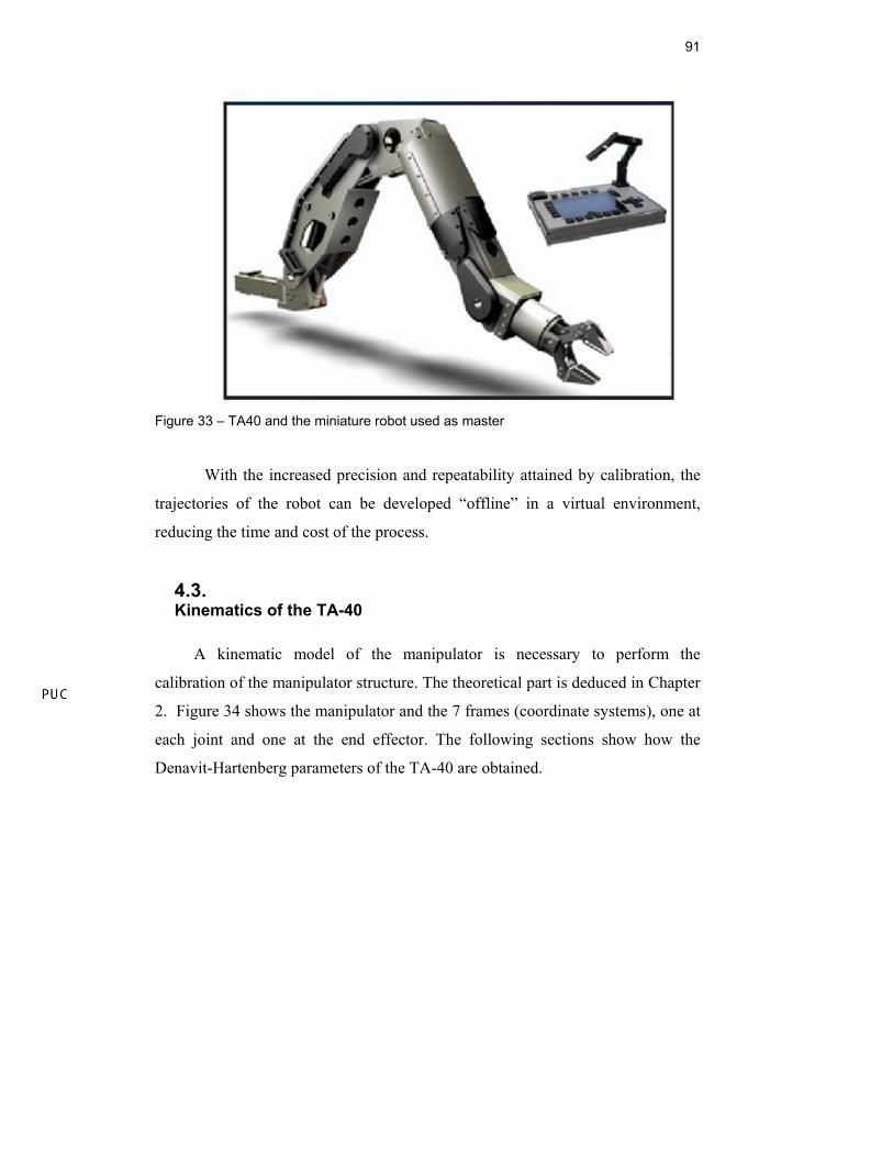
91
Figure 33 – TA40 and the miniature robot used as master
With the increased precision and repeatability attained by calibration, the
trajectories of the robot can be developed “offline” in a virtual environment,
reducing the time and cost of the process.
4.3. Kinematics of the TA-40
A kinematic model of the manipulator is necessary to perform the
calibration of the manipulator structure. The theoretical part is deduced in Chapter
2. Figure 34 shows the manipulator and the 7 frames (coordinate systems), one at
each joint and one at the end effector. The following sections show how the
Denavit-Hartenberg parameters of the TA-40 are obtained.
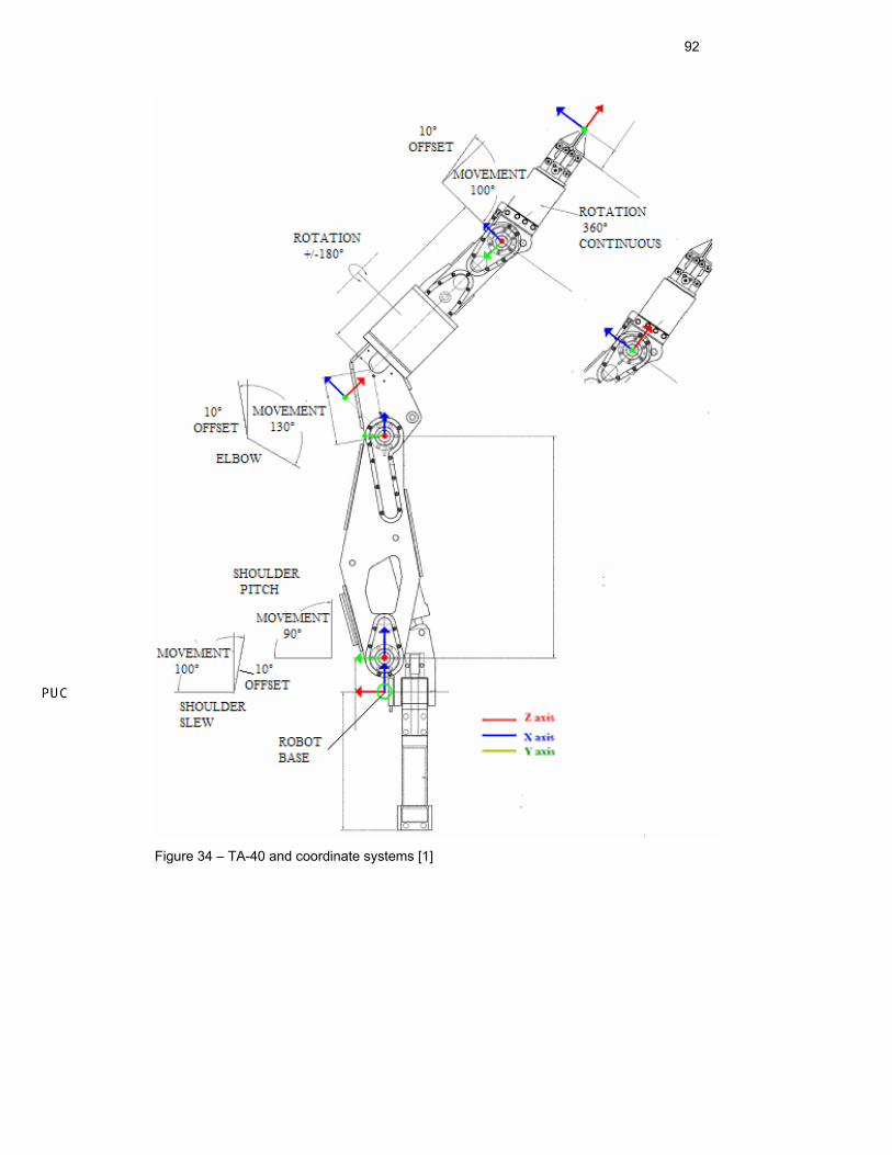
92
Figure 34 – TA-40 and coordinate systems [1]
93
4.3.1. Joints 1 and 2
The center of joint 1 (O0) is situated at the manipulator base. The axis z0
represents the rotation axis of joint 1. The axis x0 is the common normal between
the frame centers O0 of joint 1 and O1 of joint 2. The fixed distance between the
centers O0 and O1 along the common normal is 115 mm and it is represented by
a1=115 in the DH-notation. Looking in the direction of x0, the z1 axis is rotated 90º
relative to the z0 axis. This angle is represented by α1=90º. The distance between
the frame centers in direction z0 is zero, and it is represented by d1=0.
4.3.2. Joints 2 and 3
The distance between the frame centers, O1 and O2, along the common
normal is 753mm giving a2=753. The rotation axes, z1 and z2, are parallel, giving
α2=0º. The distance between O1 and O2 along z1 is zero, giving d2=0.
4.3.3. Joints 3 and 4
The distance between the frame centers is 188 mm giving a3=188. The
position of O3 is outside the structure of the manipulator. The axis z3 is rotated 90º
around the x2 axis, giving α3=90º. The distance between the respective frame
centers along z2 is zero, giving d3=0.
4.3.4. Joints 4 and 5
The frame center O4 of joint 5 is located 747mm along the z4 axis from O4,
giving d4=747. Since the frame centers position along the common normal is zero,
a4=0. The z4 axis is rotated -90º relative to z3, giving α4=-90º.
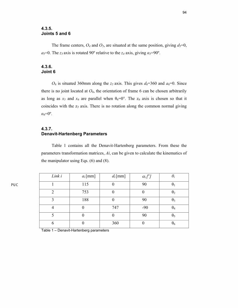
94
4.3.5. Joints 5 and 6
The frame centers, O4 and O5, are situated at the same position, giving d5=0,
a5=0. The z5 axis is rotated 90º relative to the z4 axis, giving α5=90º.
4.3.6. Joint 6
O6 is situated 360mm along the z5 axis. This gives d6=360 and a6=0. Since
there is no joint located at O6, the orientation of frame 6 can be chosen arbitrarily
as long as x5 and x6 are parallel when θ6=0°. The z6 axis is chosen so that it
coincides with the z5 axis. There is no rotation along the common normal giving
α6=0º.
4.3.7. Denavit-Hartenberg Parameters
Table 1 contains all the Denavit-Hartenberg parameters. From these the
parameters transformation matrices, Ai, can be given to calculate the kinematics of
the manipulator using Eqs. (6) and (8).
Link i ai [mm] di [mm] αi [o] θi
1 115 0 90 θ1
2 753 0 0 θ2
3 188 0 90 θ3
4 0 747 -90 θ4
5 0 0 90 θ5
6 0 360 0 θ6 Table 1 – Denavit-Hartenberg parameters
95
4.4. Calibration of the TA-40
This chapter explains how the theory in chapter 2.4 is applied to the TA-40
manipulator.
In order to estimate the generalized errors, all the redundant errors have to
be eliminated. This is done by transferring the values of the redundant errors using
Eq. (21) for i=1:6. The redundant errors εz,(i) and εr,(i) could then be eliminated for
i=0:5. The error εz,(6) cannot be eliminated since its contribution to the end-effector
position is not passed on to another joint. The errors εp,6 εs,6, and εr,6 can be
eliminated since they are rotational errors and do not effect the end-effector
position. This eliminates 15 errors in total. Further, there exists another relation
between the redundant errors given in Eq.(27). Rearranging this equation gives: *,(5) ,(5) ,(5) 6
,(5)*,(5) ,(5)
6
d
d
x x s
yp p
ε ε ε
εε ε
⎧ = + ⋅⎪⎨
= −⎪⎩
(167)
This means that εs,5, and εy,5 can be eliminated from the model, leaving only
25 errors to estimate. The reduced identification jacobian (Ge) has only 25
elements. The matrix eT
eG G is then invertible. Substituting Jt with Ge in Eq.(14)
gives a solution to the equation.
Eliminating εs,5 and associating it with the translational error means that the
orientation error of the end-effector cannot be estimated independently. Neither
can the orientation of link 5. However, the estimated orientation of link 5 will
have a fixed bias to the true orientation for all configurations of the joints. This
means that a camera on link 5 will be able to detect the pose differences between
two views.
96
4.5. Inverse Kinematics
The inverse kinematics in this chapter was deducted in [24]. It is presented
in this thesis due to the importance for automation purposes.
It is impossible to develop a general method to estimate the inverse
kinematics for a manipulator. Therefore the steps developed in this chapter cannot
be applied directly to another manipulator. Using the specific properties of the
TA-40 makes it possible to find a solution. The 5 joints 2, 3, 4, 5 and 6 are all
situated within a plane in 3D space. Their respective frames (coordinate systems)
are O1, O2, O3, O4 and O5. A graphic interpretation of this plane is given in Figure
35.
Equation (168) gives the position and orientation of the end-effector in base
coordinates.
( )0 0 1 2 3 4 56 1 2 3 4 5 6T A A A A A Aθ = (168)
Equation (168) can be elaborated to give the coordinates of frame 5, 15P ,
relative to frame 1:
( ) ( )1 11 1 0 0 5 1 2 3 45 4 1 6 6 2 3 4 5P P A T A A A A A
− −= = = (169)
Equation (162) gives the relative position and orientation of frame 5 relative
to frame 1. The frames 4 and 5 have the same position, meaning that the angle of
joint 4 does not affect the position of frame 5. By interpretation of Figure 35 the
following equations are obtained:
⎥⎥⎥⎥
⎦
⎤
⎢⎢⎢⎢
⎣
⎡++++
==
100
2342322
23423322
15
45
34
23
12
cdsasaRsdcaca
PAAAA s (170)
( ) ( )( ) ( )
( ) ( )
1 6 1 2 6 1 1
1 10 1 5 3 61 5 6
1 6 1 2 6 1
0 1
x b a c y b a s aR z b a
A P Ax b a s y b a c
− −
⎡ − + − − ⎤⎢ ⎥−⎢ ⎥=⎢ ⎥− − −⎢ ⎥⎣ ⎦
(171)
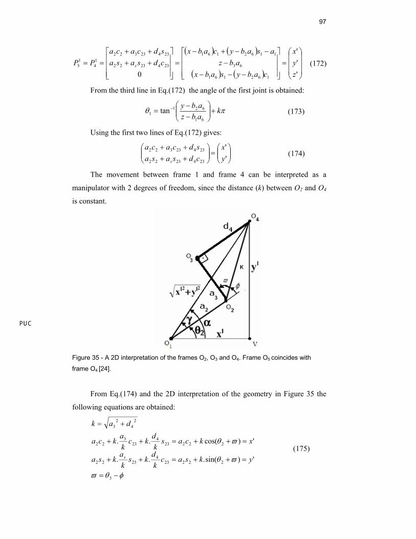
97
( ) ( )
( ) ( ) ⎟⎟⎟
⎠
⎞
⎜⎜⎜
⎝
⎛=
⎥⎥⎥
⎦
⎤
⎢⎢⎢
⎣
⎡
−−−−
−−+−=
⎥⎥⎥
⎦
⎤
⎢⎢⎢
⎣
⎡++++
=='''
0 162161
63
1162161
2342322
234233221
41
5
zyx
cabysabxabz
asabycabxcdsasasdcaca
PP s (172)
From the third line in Eq.(172) the angle of the first joint is obtained:
πθ kabzaby
+⎟⎟⎠
⎞⎜⎜⎝
⎛−−
= −
61
6211 tan (173)
Using the first two lines of Eq.(172) gives:
⎟⎟⎠
⎞⎜⎜⎝
⎛=⎟⎟
⎠
⎞⎜⎜⎝
⎛++++
''
2342322
23423322
yx
cdsasasdcaca
s
(174)
The movement between frame 1 and frame 4 can be interpreted as a
manipulator with 2 degrees of freedom, since the distance (k) between O2 and O4
is constant.
Figure 35 - A 2D interpretation of the frames O2, O3 and O4. Frame O5 coincides with
frame O4 [24].
From Eq.(174) and the 2D interpretation of the geometry in Figure 35 the
following equations are obtained:
φθϖ
ϖθ
ϖθ
−=
=++=++
=++=++
+=
3
222234
2322
222234
233
22
24
23
')sin(...
')cos(..
yksackdks
ka
ksa
xkcaskdkc
ka
kca
dak
s (175)
98
Solving the equations for θ2 and θ3 gives:
φθ +⎟⎟
⎠
⎞
⎜⎜
⎝
⎛
′+′
−+′+′+⎟⎟
⎠
⎞⎜⎜⎝
⎛= −−
222
222
221
'
'1
22
costanyxa
kayxxy (176)
⎟⎟⎠
⎞⎜⎜⎝
⎛+⎟
⎟⎠
⎞⎜⎜⎝
⎛ −−′+′−= −−
'3
41
2
222
221
3 tan2
cosad
kakayx
θ (177)
Having the angles of the first three joints and the desired position of the
end-effector, it is possible to estimate the required angles of joints 4 and 5. The
movement of joint 6 does not change the position of the end-effector, only the
orientation. The movement between frame 3 and the end-effector is given by
Eq.(178).
6 4 5
6 5 43 4 5 34 5 6 6
4 6 5
0 1
d c sR d s s
A A A Pd d c
⎡ ⎤⎢ ⎥⎢ ⎥= =⎢ ⎥+⎢ ⎥⎣ ⎦
(178)
( ) ( )1 13 0 0 1 26 3 1 2 3
''''''
1 1
x xy y
P A T A A Az z
− −
⎡ ⎤ ⎛ ⎞⎜ ⎟⎢ ⎥⎜ ⎟⎢ ⎥= = ⋅ =⎜ ⎟⎢ ⎥⎜ ⎟⎢ ⎥
⎣ ⎦ ⎝ ⎠
(179)
( )⎥⎥⎥⎥
⎦
⎤
⎢⎢⎢⎢
⎣
⎡
−+−+−−
−+++−−
=−
102312313223123
11
23123123123323
103 sasxcsasyszc
ycxsRcacxccyszscaa
TA (180)
1 23 23 1 23 23 1 23 23 3 2 3 2 3 2 33
6 1 1
1 2 3 2 3 23 23 3 12 13 2 13 2 3 12 3 2
6 4 5
6 5 4
4 6 5
(c + )+x ( - )+y (c -s )+z(s c +c )-c a -
- ( c +c s )+z( - )+x(s +c )+y(s c +c )-s a
'' ''
''
a s c c s s s aP xs yc
a s s c c s s
x d c sy d s sz d d c
⎡ ⎤⎢ ⎥= −⎢ ⎥⎢ ⎥⎣ ⎦⎛ ⎞ ⎡ ⎤⎜ ⎟ ⎢ ⎥= =⎜ ⎟ ⎢ ⎥⎜ ⎟ ⎢ ⎥+⎝ ⎠ ⎣ ⎦
(181)
All the values in Eq.(181) are constants since the angles of joints 1 to 3 have
already been found. From Eq. (181) the angles of the joints 4 and 5 are obtained:
99
πθ kxy
+⎟⎠⎞
⎜⎝⎛= −
''''tan 1
4 (182)
( )1
54 4
''tan''y
s z dθ − ⎛ ⎞
= ⎜ ⎟⎜ ⎟−⎝ ⎠ (183)
When the angles of the first five joints are obtained, the position of the end
effector is already determined. Joint six only changes the position of the end-
effector.
Therefore the angle of the sixth joint is obtained from the desired orientation of
the end effector:
⎥⎥⎥⎥
⎦
⎤
⎢⎢⎢⎢
⎣
⎡
=
1000
06 zbpn
ybpnxbpn
Azzz
yyy
xzx
(184)
( )[ ] ( )( )[ ] ( )
( ) ⎥⎥⎥
⎦
⎤
⎢⎢⎢
⎣
⎡
−++−+−++−+−+
=⎥⎥⎥
⎦
⎤
⎢⎢⎢
⎣
⎡=
642365235423
6414231652315414231
6414231652315414231
6
ssscscccssccscscssscscccsscsscccssccssccc
nnn
n
z
y
z
(185)
To simplify the equations, the following variables are introduced:
( )[ ]( )( )[ ]( )( )
4236
52354235
4142314
523154142313
4142312
523154142311
ssscccsccscs
ssscscccscsscc
ssccssccc
−=+=+−=
−+=+−=
−+=
µµµµµµ
From the angles of the joints 1 to 5 :
3241
246
1432
136
µµµµµµµµµµµµ
−−
=
−
−=
yx
yx
nnc
nns
(186)
Solving Eq.(186) gives:
1 66
6
tan 2s kc
θ π− ⎛ ⎞= +⎜ ⎟
⎝ ⎠ (187)
The inverse kinematic equations contain many trigonometric terms which
entail many possible solutions for any desired position of the end-effector.
100
Equation (173) has two solutions. Due to physical limitations, the angle of joint 1
needs to be between -10º a 90º.
Equations (176) and (177) that refer to angles θ2 and θ3 respectively have
two possible solutions each. Knowing that joint 2 only can attain positive angles
eliminates this ambiguity, allowing only solutions that give positive angles for
these joints.
Equation (182), which gives the angle of joint 4, entails a singularity when
the angle of joint 5 is zero. In this case the joints 4 and 6 are redundant. Joint 4
then has to be fixed in an arbitrary position. Joint 6 is then adjusted to give the
desired orientation of the end-effector.
101
4.6. Orientation Error of the Manipulator
According to the model of generalized errors, the exact translation and
orientation of the manipulator end-effector including errors is given by Eq.(10).
When the manipulator structure has been calibrated, the end effector position can
be estimated. However, the orientation of the end-effector cannot be estimated
accurately since the rotary error ,5sε has been eliminated and transferred to the
translational error ,5xε . Also, the translational error ,5yε has been eliminated and
transferred to the rotary error ,5pε . This gives the right position, but the translation
error of the end effector is not possible to estimate using the reduced set of errors.
If the camera is placed on link 5 of the manipulator, it is the rotation error of link
5 that needs to be considered. The homogeneous matrix 4x4 that describes the
orientation and position of the link 5 relative to its base as a function of the angles
of the joints θ=[θ1 θ2 θ3 θ4 θ5 θ6] and the generalized errors ε is given by:
0 0 1 2 3 4
5 0 1 1 2 2 3 3 4 4 5( , )T E A E A E A E A E Aθ ε = (188)
This equation gives the actual position and orientation of link 5 given a full
set of generalized errors. After the calibration of the robot, only the independent
subset, ε· is available. This means that the eliminated errors of ε have to be
substituted by zeros in the generalized error matrices. The deviation between the
true and estimated orientation and position can then be given by:
050
0 0 , 1 0 55 5 5 0
5
( , ) ( , )
0 0 0 1
XR Y
T T TZ
θ ε θ ε−
⎡ ⎤∆⎢ ⎥∆ ∆⎢ ⎥∆ = =⎢ ⎥∆⎢ ⎥⎣ ⎦
(189)
The nature of the deviation can be visualized in a simulation. By first
defining a full 1 x 42 error vector and then estimating the reduced set of errors, the
effects can be simulated.
102
5 0 5 5
5 5 5 5
5 0 5 5
11 12 13
21 22 23
31 32 33
cos 0 sin cos sin 0 1 0 00 1 0 sin cos 0 0 cos sin
sin 0 cos 0 0 1 0 sin cos
y y x x
x x z z
y y z z
R
R R RR R RR R R
θ θ θ θ
θ θ θ θθ θ θ θ
⎡ ⎤∆ ∆ ∆ − ∆⎡ ⎤ ⎡ ⎤⎢ ⎥⎢ ⎥ ⎢ ⎥
∆ = ⋅ ∆ ∆ ⋅ ∆ − ∆⎢ ⎥⎢ ⎥ ⎢ ⎥⎢ ⎥⎢ ⎥ ⎢ ⎥− ∆ ∆ ∆ ∆⎢ ⎥⎣ ⎦ ⎣ ⎦ ⎣ ⎦
∆ ∆ ∆⎡ ⎤⎢ ⎥= ∆ ∆ ∆⎢ ⎥⎢ ⎥∆ ∆ ∆⎣ ⎦
(190)
The final expression for the relative rotation matrix will be:
5 5 5 5 5
5 5
5 5 5 5 5
5 5 5 5 5
5 5
11
21
31
12
22
32
cos cos sin sin sin
sin cos
sin cos sin cos sin
cos sin sin sin cos
cos cos
sin
y z x y z
z x
y z x y z
y z x y z
x z
RRR
RRR
θ θ θ θ θ
θ θ
θ θ θ θ θ
θ θ θ θ θ
θ θ
θ
⎡ ⎤∆ ∆ − ∆ ∆ ∆∆⎡ ⎤⎢ ⎥⎢ ⎥∆ = − ∆ ∆⎢ ⎥⎢ ⎥⎢ ⎥⎢ ⎥∆ ∆ ∆ + ∆ ∆ ∆⎣ ⎦ ⎢ ⎥⎣ ⎦
∆ ∆ + ∆ ∆ ∆∆⎡ ⎤⎢ ⎥∆ = ∆ ∆⎢ ⎥⎢ ⎥∆ ∆⎣ ⎦
5 5 5 5 5
5 5
5
5 5
13
23
33
cos sin cos cos
sin cos
sin
cos cos
x z x y z
y x
x
y x
RRR
θ θ θ θ
θ θ
θ
θ θ
⎡ ⎤⎢ ⎥⎢ ⎥⎢ ⎥∆ − ∆ ∆ ∆⎢ ⎥⎣ ⎦⎡ ⎤− ∆ ∆∆⎡ ⎤⎢ ⎥⎢ ⎥∆ = ∆⎢ ⎥⎢ ⎥⎢ ⎥⎢ ⎥∆ ∆ ∆⎣ ⎦ ⎢ ⎥⎣ ⎦
(191)
From Eq.(191) the relative rotation angles can be determined.
5
1 13
33
tanyRR
θ − ⎛ ⎞∆∆ = −⎜ ⎟∆⎝ ⎠
(192)
( )5
12,3sinx Rθ −∆ = ∆ (193)
5
1 21
22
tanzRR
θ − ⎛ ⎞∆∆ = −⎜ ⎟∆⎝ ⎠
(194)
To get an idea of the magnitude of the orientation errors of link 5 there a
simulation was performed. The actual generalized position errors were chosen
randomly in the interval +/- 2 mm and the rotational errors in the interval +/- 1° =
+/- π/180 radians. 100 measurements of the end-effector were simulated and the
reduced error vector, ε·, was estimated.
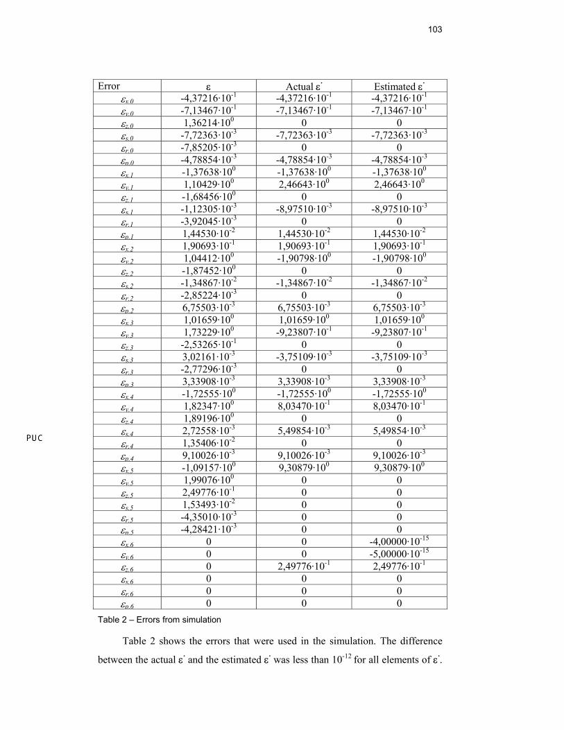
103
Error ε Actual ε· Estimated ε· εx,0 -4,37216·10-1 -4,37216·10-1 -4,37216·10-1 εy.0 -7,13467·10-1 -7,13467·10-1 -7,13467·10-1 εz.0 1,36214·100 0 0 εs.0 -7,72363·10-3 -7,72363·10-3 -7,72363·10-3 εr.0 -7,85205·10-3 0 0 εp.0 -4,78854·10-3 -4,78854·10-3 -4,78854·10-3 εx.1 -1,37638·100 -1,37638·100 -1,37638·100 εy.1 1,10429·100 2,46643·100 2,46643·100 εz.1 -1,68456·100 0 0 εs.1 -1,12305·10-3 -8,97510·10-3 -8,97510·10-3 εr.1 -3,92045·10-3 0 0 εp.1 1,44530·10-2 1,44530·10-2 1,44530·10-2 εx.2 1,90693·10-1 1,90693·10-1 1,90693·10-1 εy.2 1,04412·100 -1,90798·100 -1,90798·100 εz.2 -1,87452·100 0 0 εs.2 -1,34867·10-2 -1,34867·10-2 -1,34867·10-2 εr.2 -2,85224·10-3 0 0 εp.2 6,75503·10-3 6,75503·10-3 6,75503·10-3 εx.3 1,01659·100 1,01659·100 1,01659·100 εy.3 1,73229·100 -9,23807·10-1 -9,23807·10-1 εz.3 -2,53265·10-1 0 0 εs.3 3,02161·10-3 -3,75109·10-3 -3,75109·10-3 εr.3 -2,77296·10-3 0 0 εp.3 3,33908·10-3 3,33908·10-3 3,33908·10-3 εx.4 -1,72555·100 -1,72555·100 -1,72555·100 εy.4 1,82347·100 8,03470·10-1 8,03470·10-1 εz.4 1,89196·100 0 0 εs.4 2,72558·10-3 5,49854·10-3 5,49854·10-3 εr.4 1,35406·10-2 0 0 εp.4 9,10026·10-3 9,10026·10-3 9,10026·10-3 εx.5 -1,09157·100 9,30879·100 9,30879·100 εy.5 1,99076·100 0 0 εz.5 2,49776·10-1 0 0 εs.5 1,53493·10-2 0 0 εr.5 -4,35010·10-3 0 0 εp.5 -4,28421·10-3 0 0 εx.6 0 0 -4,00000·10-15 εy.6 0 0 -5,00000·10-15 εz.6 0 2,49776·10-1 2,49776·10-1 εs.6 0 0 0 εr.6 0 0 0 εp.6 0 0 0
Table 2 – Errors from simulation
Table 2 shows the errors that were used in the simulation. The difference
between the actual ε· and the estimated ε· was less than 10-12 for all elements of ε·.
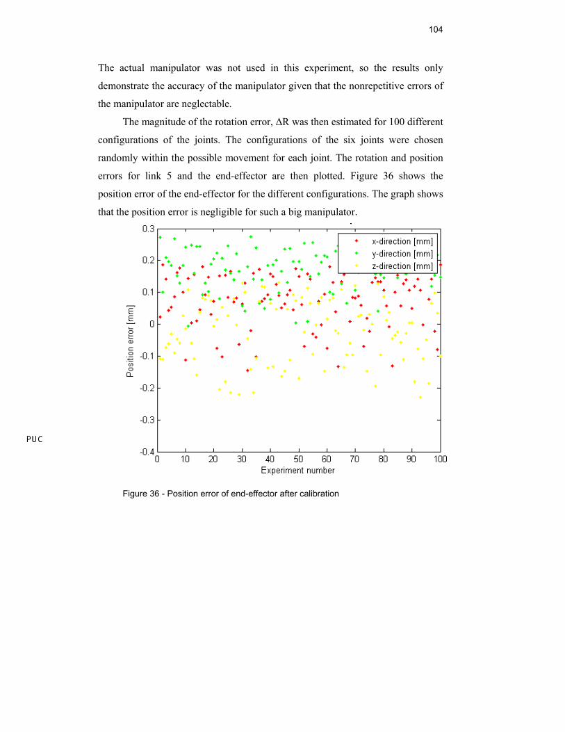
104
The actual manipulator was not used in this experiment, so the results only
demonstrate the accuracy of the manipulator given that the nonrepetitive errors of
the manipulator are neglectable.
The magnitude of the rotation error, ∆R was then estimated for 100 different
configurations of the joints. The configurations of the six joints were chosen
randomly within the possible movement for each joint. The rotation and position
errors for link 5 and the end-effector are then plotted. Figure 36 shows the
position error of the end-effector for the different configurations. The graph shows
that the position error is negligible for such a big manipulator.
Figure 36 - Position error of end-effector after calibration
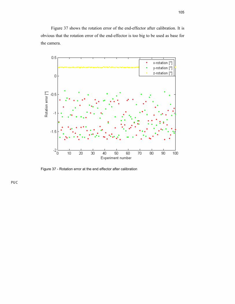
105
Figure 37 shows the rotation error of the end-effector after calibration. It is
obvious that the rotation error of the end-effector is too big to be used as base for
the camera.
Figure 37 - Rotation error at the end effector after calibration
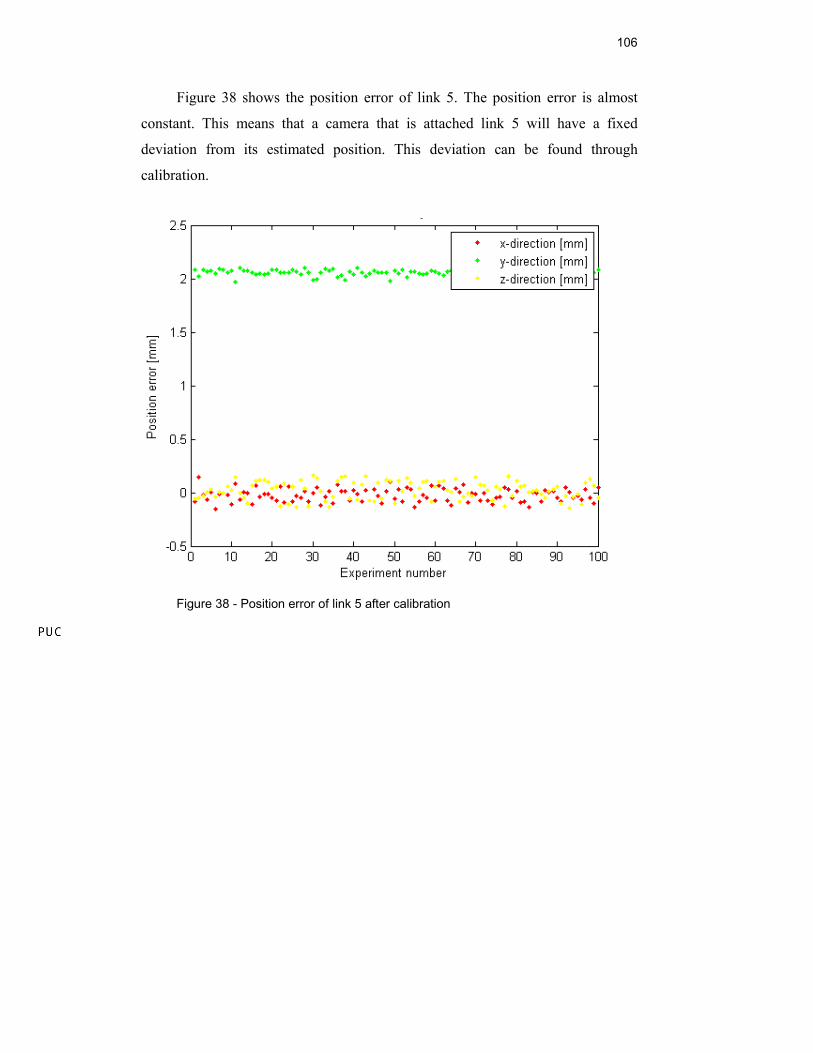
106
Figure 38 shows the position error of link 5. The position error is almost
constant. This means that a camera that is attached link 5 will have a fixed
deviation from its estimated position. This deviation can be found through
calibration.
Figure 38 - Position error of link 5 after calibration
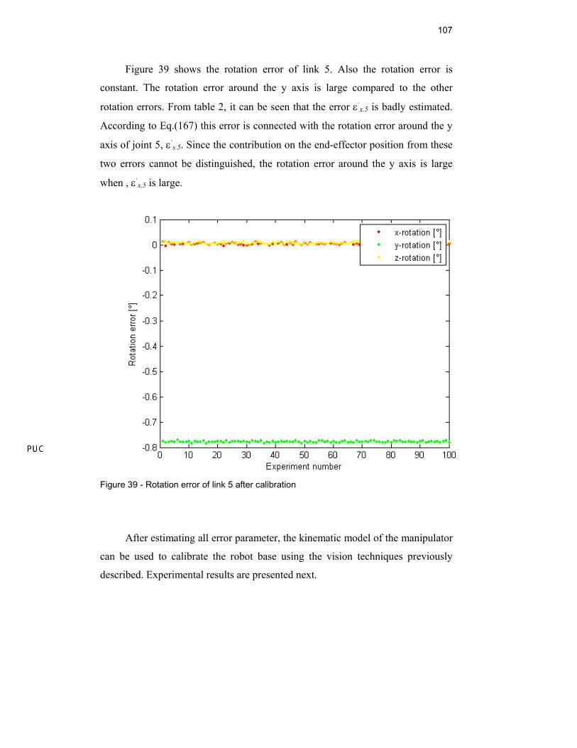
107
Figure 39 shows the rotation error of link 5. Also the rotation error is
constant. The rotation error around the y axis is large compared to the other
rotation errors. From table 2, it can be seen that the error ε·x.5 is badly estimated.
According to Eq.(167) this error is connected with the rotation error around the y
axis of joint 5, ε·s.5. Since the contribution on the end-effector position from these
two errors cannot be distinguished, the rotation error around the y axis is large
when , ε·x,5 is large.
Figure 39 - Rotation error of link 5 after calibration
After estimating all error parameter, the kinematic model of the manipulator
can be used to calibrate the robot base using the vision techniques previously
described. Experimental results are presented next.
5 Results
5.1. Introduction
The objective of this chapter is to implement the presented theory in
practical experiments. The theory was first simulated in Matlab in order to
eliminate errors in the mathematic models and to make it easier to identify
potential anomalies in the experiments. These experiments were performed in the
robotic laboratory at PUC-Rio.
5.2. Laboratory Experiments
These experiments were carried out using an x-y table with a movement
range of 200mm in x and y directions and a resolution of 0.1mm. A rotary stage is
mounted on top of the x-y table. The rotation axis is perpendicular to the x-y table
and the angular resolution is 0.1°. A camera was mounted on the rotary stage. The
table with the mounted web camera is shown in Figure 40.
The camera calibration was performed using a 2D calibration rig with two
perpendicular planes with 7 x 7 squares in chess pattern. The chess boards had
dimensions 197mm x 197mm. The calibration rig is shown in Figure 41.
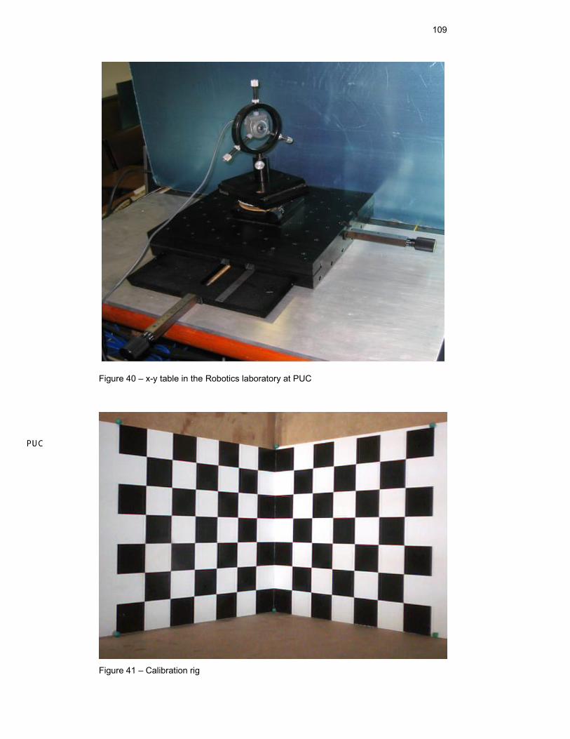
109
Figure 40 – x-y table in the Robotics laboratory at PUC
Figure 41 – Calibration rig
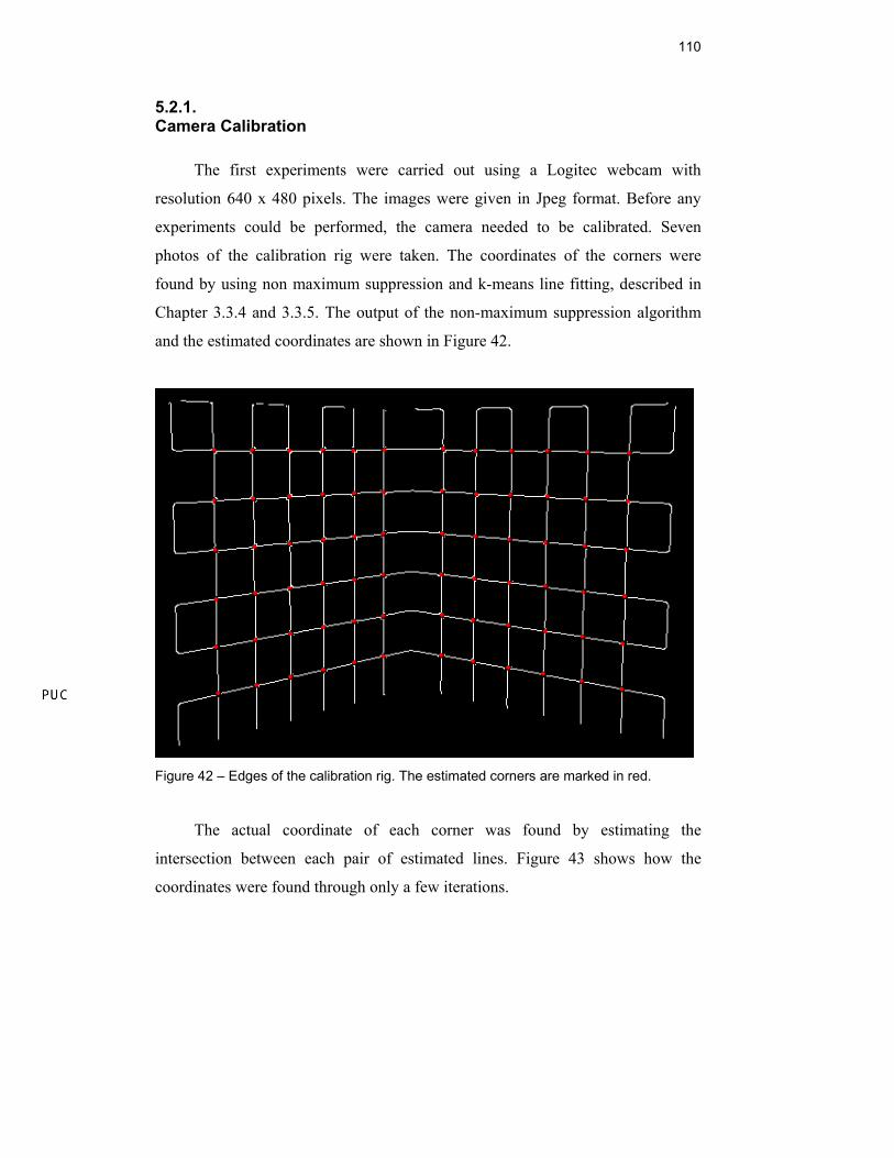
110
5.2.1. Camera Calibration
The first experiments were carried out using a Logitec webcam with
resolution 640 x 480 pixels. The images were given in Jpeg format. Before any
experiments could be performed, the camera needed to be calibrated. Seven
photos of the calibration rig were taken. The coordinates of the corners were
found by using non maximum suppression and k-means line fitting, described in
Chapter 3.3.4 and 3.3.5. The output of the non-maximum suppression algorithm
and the estimated coordinates are shown in Figure 42.
Figure 42 – Edges of the calibration rig. The estimated corners are marked in red.
The actual coordinate of each corner was found by estimating the
intersection between each pair of estimated lines. Figure 43 shows how the
coordinates were found through only a few iterations.
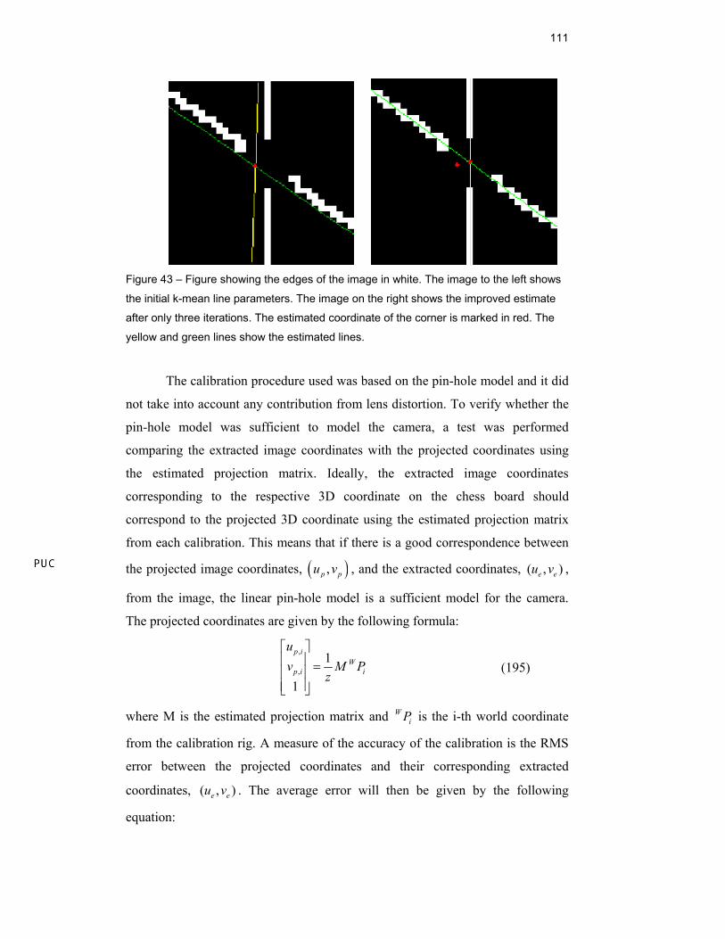
111
Figure 43 – Figure showing the edges of the image in white. The image to the left shows
the initial k-mean line parameters. The image on the right shows the improved estimate
after only three iterations. The estimated coordinate of the corner is marked in red. The
yellow and green lines show the estimated lines.
The calibration procedure used was based on the pin-hole model and it did
not take into account any contribution from lens distortion. To verify whether the
pin-hole model was sufficient to model the camera, a test was performed
comparing the extracted image coordinates with the projected coordinates using
the estimated projection matrix. Ideally, the extracted image coordinates
corresponding to the respective 3D coordinate on the chess board should
correspond to the projected 3D coordinate using the estimated projection matrix
from each calibration. This means that if there is a good correspondence between
the projected image coordinates, ( ),p pu v , and the extracted coordinates, ( , )e eu v ,
from the image, the linear pin-hole model is a sufficient model for the camera.
The projected coordinates are given by the following formula:
,
,1
1
p iW
p i i
uv M P
z
⎡ ⎤⎢ ⎥ =⎢ ⎥⎢ ⎥⎣ ⎦
(195)
where M is the estimated projection matrix and WiP is the i-th world coordinate
from the calibration rig. A measure of the accuracy of the calibration is the RMS
error between the projected coordinates and their corresponding extracted
coordinates, ( , )e eu v . The average error will then be given by the following
equation:
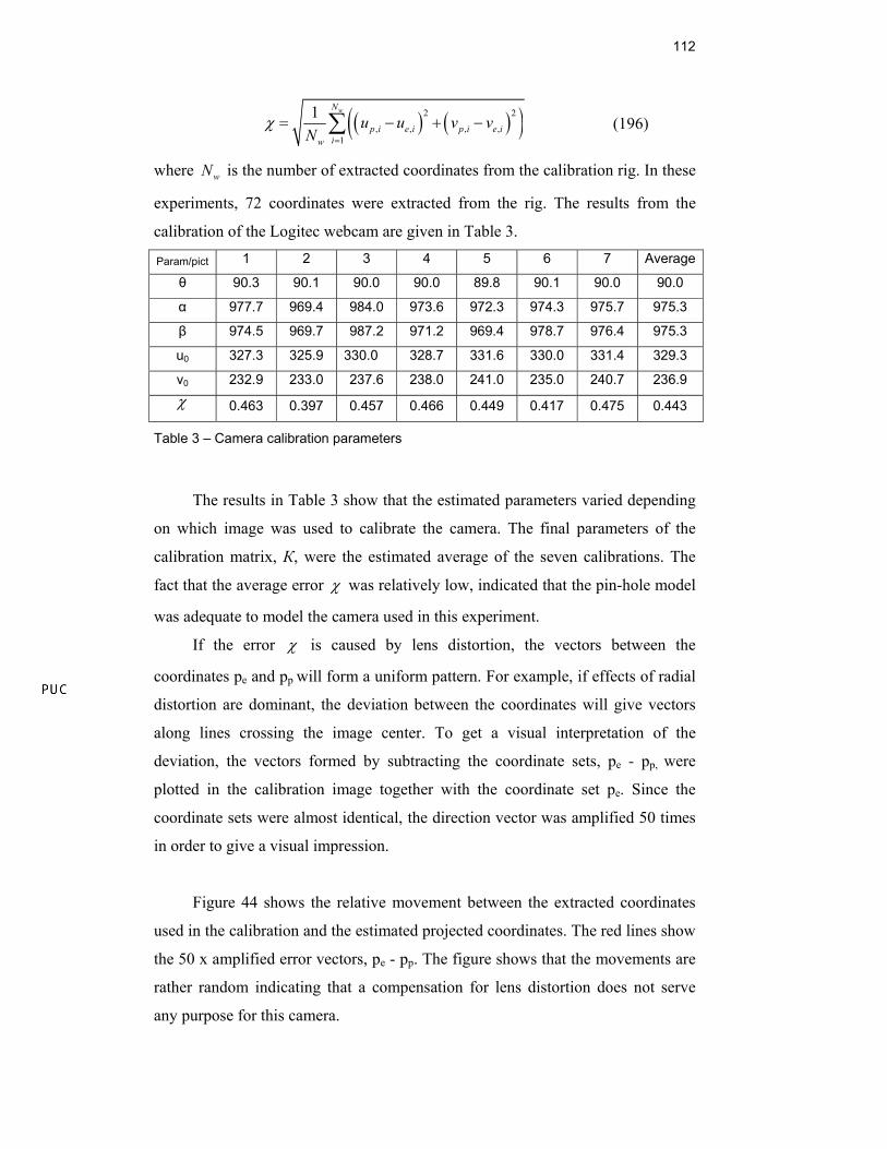
112
( ) ( )( )2 2
, , , ,1
1 wN
p i e i p i e iiw
u u v vN
χ=
= − + −∑ (196)
where wN is the number of extracted coordinates from the calibration rig. In these
experiments, 72 coordinates were extracted from the rig. The results from the
calibration of the Logitec webcam are given in Table 3.
Param/pict 1 2 3 4 5 6 7 Average
θ 90.3 90.1 90.0 90.0 89.8 90.1 90.0 90.0
α 977.7 969.4 984.0 973.6 972.3 974.3 975.7 975.3
β 974.5 969.7 987.2 971.2 969.4 978.7 976.4 975.3
u0 327.3 325.9 330.0 328.7 331.6 330.0 331.4 329.3
v0 232.9 233.0 237.6 238.0 241.0 235.0 240.7 236.9 χ 0.463 0.397 0.457 0.466 0.449 0.417 0.475 0.443
Table 3 – Camera calibration parameters
The results in Table 3 show that the estimated parameters varied depending
on which image was used to calibrate the camera. The final parameters of the
calibration matrix, К, were the estimated average of the seven calibrations. The
fact that the average error χ was relatively low, indicated that the pin-hole model
was adequate to model the camera used in this experiment.
If the error χ is caused by lens distortion, the vectors between the
coordinates pe and pp will form a uniform pattern. For example, if effects of radial
distortion are dominant, the deviation between the coordinates will give vectors
along lines crossing the image center. To get a visual interpretation of the
deviation, the vectors formed by subtracting the coordinate sets, pe - pp, were
plotted in the calibration image together with the coordinate set pe. Since the
coordinate sets were almost identical, the direction vector was amplified 50 times
in order to give a visual impression.
Figure 44 shows the relative movement between the extracted coordinates
used in the calibration and the estimated projected coordinates. The red lines show
the 50 x amplified error vectors, pe - pp. The figure shows that the movements are
rather random indicating that a compensation for lens distortion does not serve
any purpose for this camera.
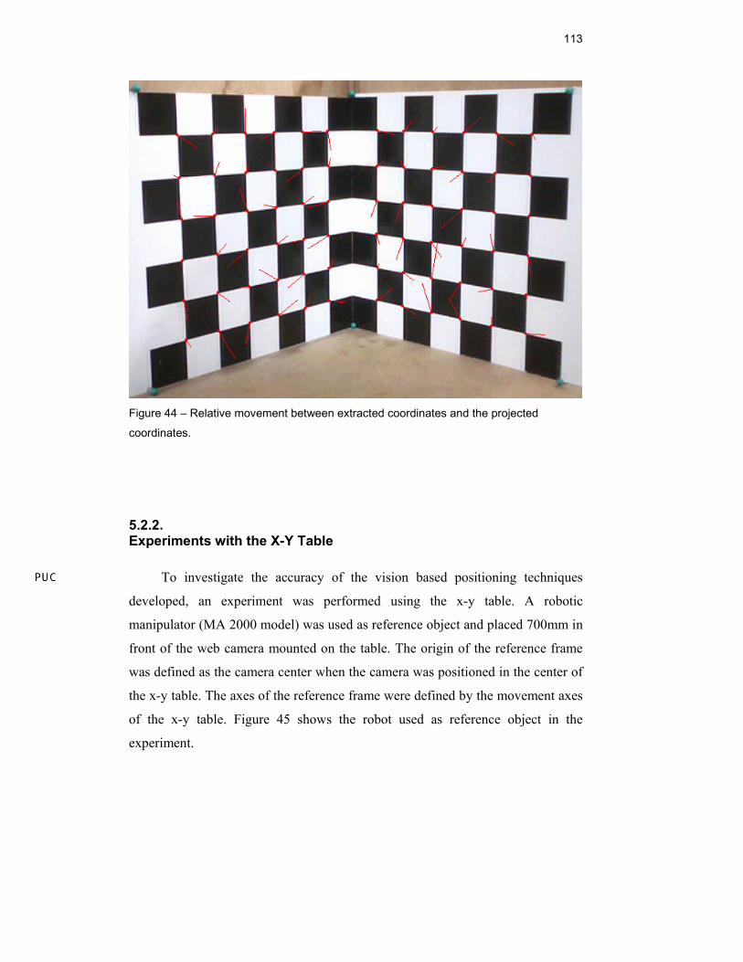
113
Figure 44 – Relative movement between extracted coordinates and the projected
coordinates.
5.2.2. Experiments with the X-Y Table
To investigate the accuracy of the vision based positioning techniques
developed, an experiment was performed using the x-y table. A robotic
manipulator (MA 2000 model) was used as reference object and placed 700mm in
front of the web camera mounted on the table. The origin of the reference frame
was defined as the camera center when the camera was positioned in the center of
the x-y table. The axes of the reference frame were defined by the movement axes
of the x-y table. Figure 45 shows the robot used as reference object in the
experiment.
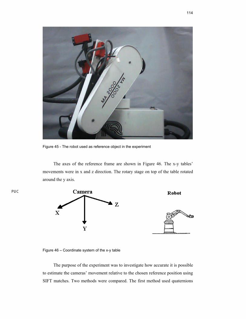
114
Figure 45 - The robot used as reference object in the experiment
The axes of the reference frame are shown in Figure 46. The x-y tables’
movements were in x and z direction. The rotary stage on top of the table rotated
around the y axis.
Figure 46 – Coordinate system of the x-y table
The purpose of the experiment was to investigate how accurate it is possible
to estimate the cameras’ movement relative to the chosen reference position using
SIFT matches. Two methods were compared. The first method used quaternions
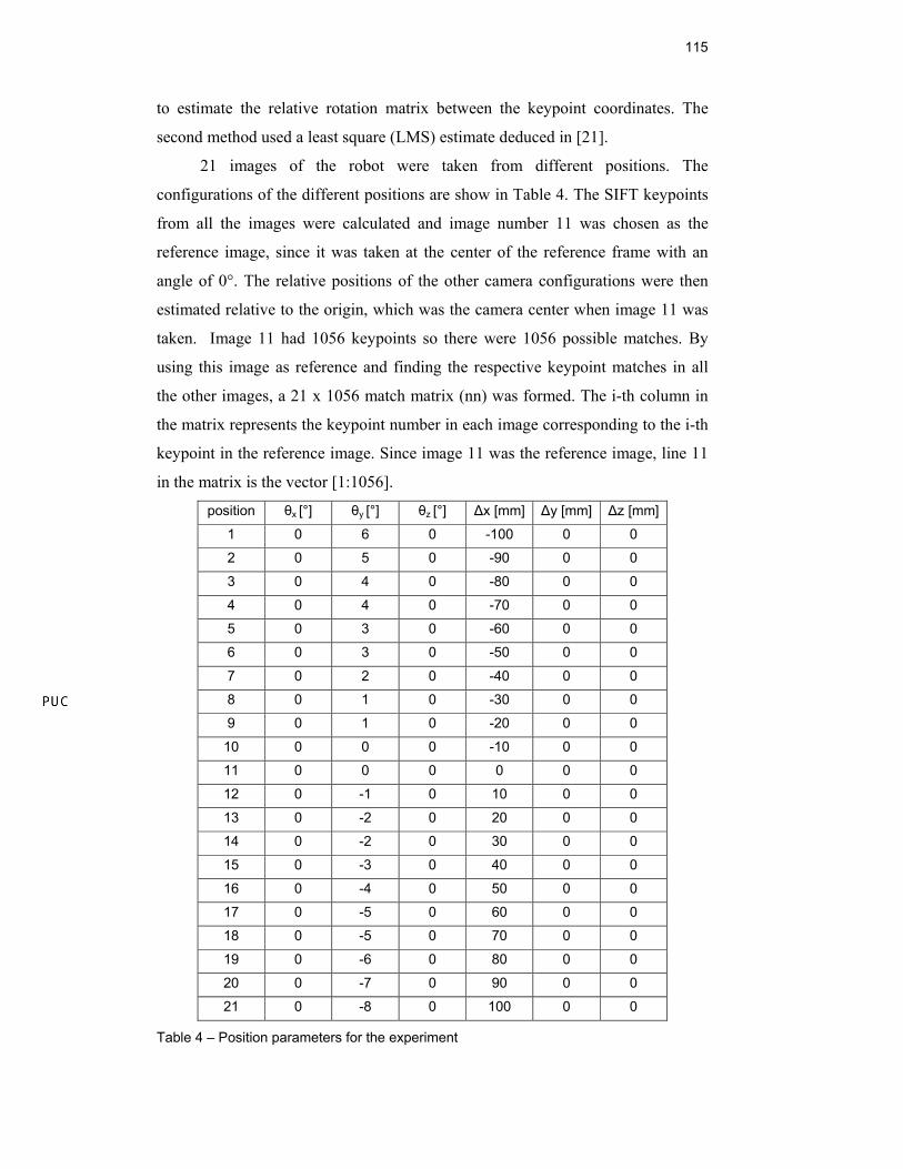
115
to estimate the relative rotation matrix between the keypoint coordinates. The
second method used a least square (LMS) estimate deduced in [21].
21 images of the robot were taken from different positions. The
configurations of the different positions are show in Table 4. The SIFT keypoints
from all the images were calculated and image number 11 was chosen as the
reference image, since it was taken at the center of the reference frame with an
angle of 0°. The relative positions of the other camera configurations were then
estimated relative to the origin, which was the camera center when image 11 was
taken. Image 11 had 1056 keypoints so there were 1056 possible matches. By
using this image as reference and finding the respective keypoint matches in all
the other images, a 21 x 1056 match matrix (nn) was formed. The i-th column in
the matrix represents the keypoint number in each image corresponding to the i-th
keypoint in the reference image. Since image 11 was the reference image, line 11
in the matrix is the vector [1:1056].
position θx [°] θy [°] θz [°] ∆x [mm] ∆y [mm] ∆z [mm]
1 0 6 0 -100 0 0
2 0 5 0 -90 0 0
3 0 4 0 -80 0 0
4 0 4 0 -70 0 0
5 0 3 0 -60 0 0
6 0 3 0 -50 0 0
7 0 2 0 -40 0 0
8 0 1 0 -30 0 0
9 0 1 0 -20 0 0
10 0 0 0 -10 0 0
11 0 0 0 0 0 0
12 0 -1 0 10 0 0
13 0 -2 0 20 0 0
14 0 -2 0 30 0 0
15 0 -3 0 40 0 0
16 0 -4 0 50 0 0
17 0 -5 0 60 0 0
18 0 -5 0 70 0 0
19 0 -6 0 80 0 0
20 0 -7 0 90 0 0
21 0 -8 0 100 0 0
Table 4 – Position parameters for the experiment
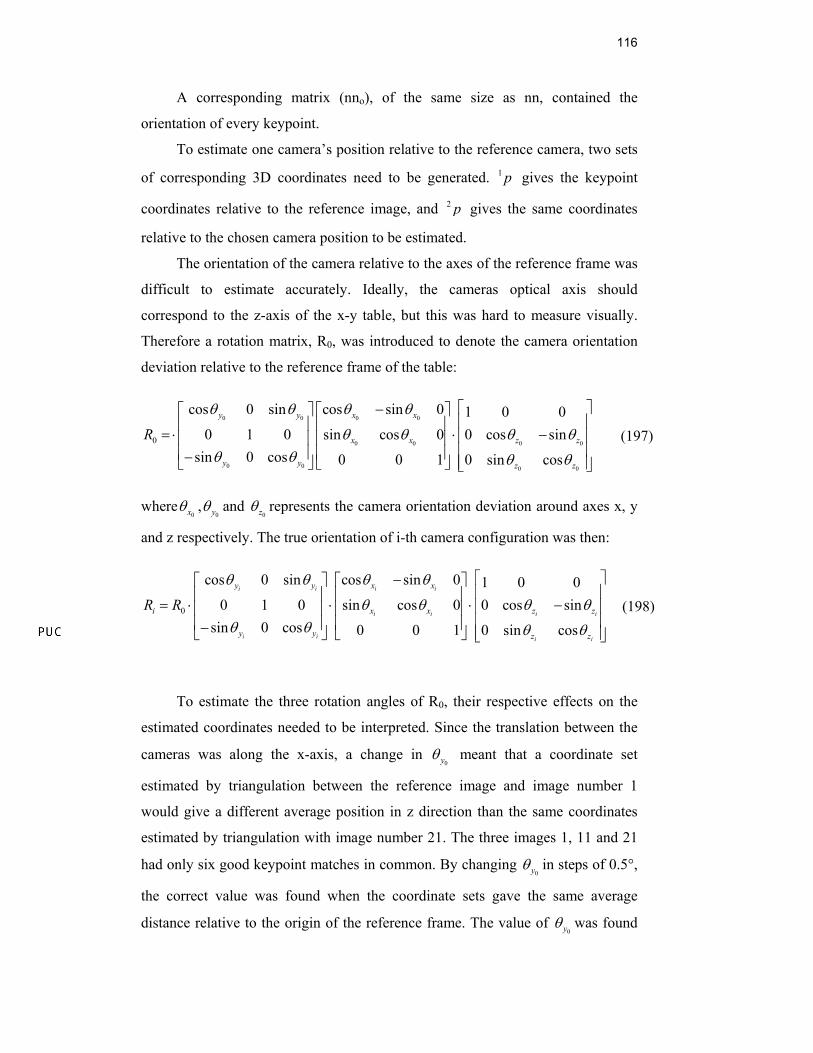
116
A corresponding matrix (nno), of the same size as nn, contained the
orientation of every keypoint.
To estimate one camera’s position relative to the reference camera, two sets
of corresponding 3D coordinates need to be generated. 1 p gives the keypoint
coordinates relative to the reference image, and 2 p gives the same coordinates
relative to the chosen camera position to be estimated.
The orientation of the camera relative to the axes of the reference frame was
difficult to estimate accurately. Ideally, the cameras optical axis should
correspond to the z-axis of the x-y table, but this was hard to measure visually.
Therefore a rotation matrix, R0, was introduced to denote the camera orientation
deviation relative to the reference frame of the table:
0 0 0 0
0 0 0 0
0 0 0 0
0
cos 0 sin cos sin 0 1 0 00 1 0 sin cos 0 0 cos sin
sin 0 cos 0 0 1 0 sin cos
y y x x
x x z z
y y z z
R
θ θ θ θ
θ θ θ θθ θ θ θ
⎡ ⎤−⎡ ⎤ ⎡ ⎤⎢ ⎥⎢ ⎥ ⎢ ⎥
= ⋅ ⋅ −⎢ ⎥⎢ ⎥ ⎢ ⎥⎢ ⎥⎢ ⎥ ⎢ ⎥− ⎢ ⎥⎣ ⎦ ⎣ ⎦ ⎣ ⎦
(197)
where0xθ ,
0yθ and 0zθ represents the camera orientation deviation around axes x, y
and z respectively. The true orientation of i-th camera configuration was then:
0
cos 0 sin cos sin 0 1 0 00 1 0 sin cos 0 0 cos sin
sin 0 cos 0 0 1 0 sin cos
i i i i
i i i i
i i i i
y y x x
i x x z z
y y z z
R R
θ θ θ θ
θ θ θ θθ θ θ θ
⎡ ⎤−⎡ ⎤ ⎡ ⎤⎢ ⎥⎢ ⎥ ⎢ ⎥
= ⋅ ⋅ ⋅ −⎢ ⎥⎢ ⎥ ⎢ ⎥⎢ ⎥⎢ ⎥ ⎢ ⎥− ⎢ ⎥⎣ ⎦ ⎣ ⎦ ⎣ ⎦
(198)
To estimate the three rotation angles of R0, their respective effects on the
estimated coordinates needed to be interpreted. Since the translation between the
cameras was along the x-axis, a change in 0yθ meant that a coordinate set
estimated by triangulation between the reference image and image number 1
would give a different average position in z direction than the same coordinates
estimated by triangulation with image number 21. The three images 1, 11 and 21
had only six good keypoint matches in common. By changing 0yθ in steps of 0.5°,
the correct value was found when the coordinate sets gave the same average
distance relative to the origin of the reference frame. The value of 0yθ was found
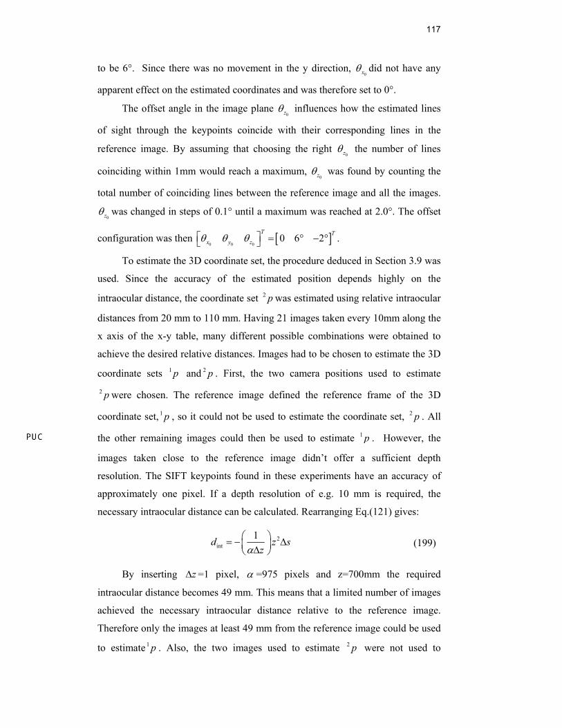
117
to be 6°. Since there was no movement in the y direction, 0xθ did not have any
apparent effect on the estimated coordinates and was therefore set to 0°.
The offset angle in the image plane 0zθ influences how the estimated lines
of sight through the keypoints coincide with their corresponding lines in the
reference image. By assuming that choosing the right 0zθ the number of lines
coinciding within 1mm would reach a maximum, 0zθ was found by counting the
total number of coinciding lines between the reference image and all the images.
0zθ was changed in steps of 0.1° until a maximum was reached at 2.0°. The offset
configuration was then [ ]0 0 0
0 6° 2°T T
x y zθ θ θ⎡ ⎤ = −⎣ ⎦ .
To estimate the 3D coordinate set, the procedure deduced in Section 3.9 was
used. Since the accuracy of the estimated position depends highly on the
intraocular distance, the coordinate set 2 p was estimated using relative intraocular
distances from 20 mm to 110 mm. Having 21 images taken every 10mm along the
x axis of the x-y table, many different possible combinations were obtained to
achieve the desired relative distances. Images had to be chosen to estimate the 3D
coordinate sets 1 p and 2 p . First, the two camera positions used to estimate 2 p were chosen. The reference image defined the reference frame of the 3D
coordinate set, 1 p , so it could not be used to estimate the coordinate set, 2 p . All
the other remaining images could then be used to estimate 1 p . However, the
images taken close to the reference image didn’t offer a sufficient depth
resolution. The SIFT keypoints found in these experiments have an accuracy of
approximately one pixel. If a depth resolution of e.g. 10 mm is required, the
necessary intraocular distance can be calculated. Rearranging Eq.(121) gives:
2int
1d z szα
⎛ ⎞= − ∆⎜ ⎟∆⎝ ⎠ (199)
By inserting z∆ =1 pixel, α =975 pixels and z=700mm the required
intraocular distance becomes 49 mm. This means that a limited number of images
achieved the necessary intraocular distance relative to the reference image.
Therefore only the images at least 49 mm from the reference image could be used
to estimate1 p . Also, the two images used to estimate 2 p were not used to
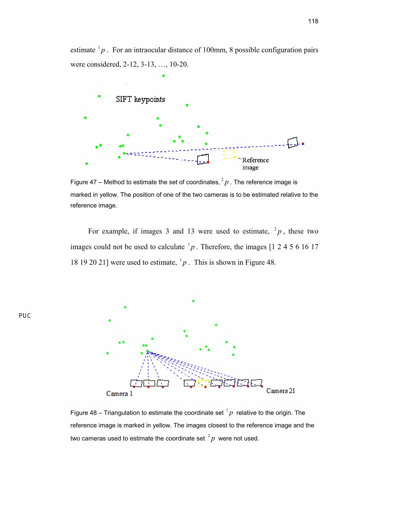
118
estimate 1 p . For an intraocular distance of 100mm, 8 possible configuration pairs
were considered, 2-12, 3-13, …, 10-20.
Figure 47 – Method to estimate the set of coordinates, 2 p . The reference image is
marked in yellow. The position of one of the two cameras is to be estimated relative to the
reference image.
For example, if images 3 and 13 were used to estimate, 2 p , these two
images could not be used to calculate 1 p . Therefore, the images [1 2 4 5 6 16 17
18 19 20 21] were used to estimate, 1 p . This is shown in Figure 48.
Figure 48 – Triangulation to estimate the coordinate set 1 p relative to the origin. The
reference image is marked in yellow. The images closest to the reference image and the
two cameras used to estimate the coordinate set 2 p were not used.
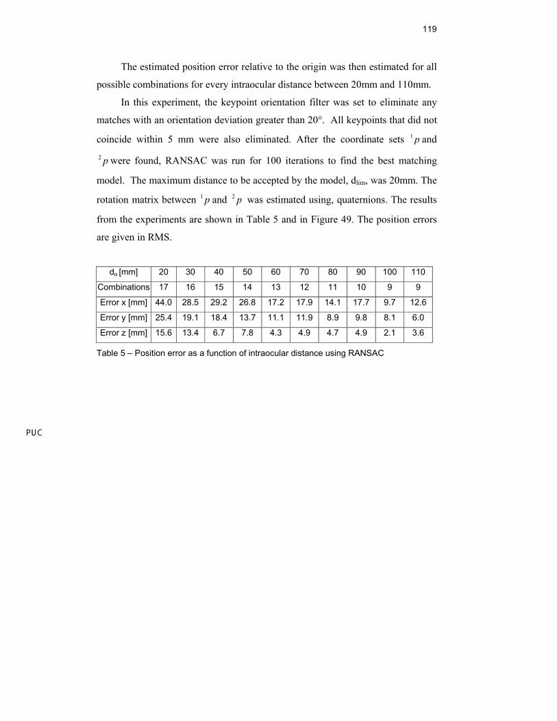
119
The estimated position error relative to the origin was then estimated for all
possible combinations for every intraocular distance between 20mm and 110mm.
In this experiment, the keypoint orientation filter was set to eliminate any
matches with an orientation deviation greater than 20°. All keypoints that did not
coincide within 5 mm were also eliminated. After the coordinate sets 1 p and 2 p were found, RANSAC was run for 100 iterations to find the best matching
model. The maximum distance to be accepted by the model, dlim, was 20mm. The
rotation matrix between 1 p and 2 p was estimated using, quaternions. The results
from the experiments are shown in Table 5 and in Figure 49. The position errors
are given in RMS.
Table 5 – Position error as a function of intraocular distance using RANSAC
do [mm] 20 30 40 50 60 70 80 90 100 110
Combinations 17 16 15 14 13 12 11 10 9 9
Error x [mm] 44.0 28.5 29.2 26.8 17.2 17.9 14.1 17.7 9.7 12.6
Error y [mm] 25.4 19.1 18.4 13.7 11.1 11.9 8.9 9.8 8.1 6.0
Error z [mm] 15.6 13.4 6.7 7.8 4.3 4.9 4.7 4.9 2.1 3.6
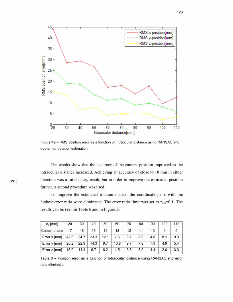
120
Figure 49 – RMS position error as a function of intraocular distance using RANSAC and
quaternion rotation estimation.
The results show that the accuracy of the camera position improved as the
intraocular distance increased. Achieving an accuracy of close to 10 mm in either
direction was a satisfactory result, but in order to improve the estimated position
further, a second procedure was used.
To improve the estimated rotation matrix, the coordinate pairs with the
highest error ratio were eliminated. The error ratio limit was set to rlim=0.1. The
results can be seen in Table 6 and in Figure 50.
Table 6 – Position error as a function of intraocular distance using RANSAC and error
ratio elimination.
do [mm] 20 30 40 50 60 70 80 90 100 110
Combinations 17 16 15 14 13 12 11 10 9 9
Error x [mm] 42.6 24.7 23.3 12.1 7.6 9.7 8.9 4.8 8.1 9.3
Error y [mm] 26.2 22.9 14.3 9.7 10.8 9.7 7.8 7.9 4.9 5.4
Error z [mm] 15.0 11.4 6.7 6.2 4.5 3.5 5.0 4.4 2.0 3.3
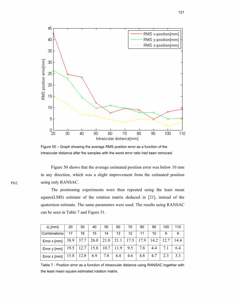
121
Figure 50 – Graph showing the average RMS position error as a function of the
intraocular distance after the samples with the worst error ratio had been removed.
Figure 50 shows that the average estimated position error was below 10 mm
in any direction, which was a slight improvement from the estimated position
using only RANSAC.
The positioning experiments were then repeated using the least mean
square(LMS) estimate of the rotation matrix deduced in [21], instead of the
quaternion estimate. The same parameters were used. The results using RANSAC
can be seen in Table 7 and Figure 51.
Table 7 - Position error as a function of intraocular distance using RANSAC together with
the least mean square estimated rotation matrix.
do [mm] 20 30 40 50 60 70 80 90 100 110
Combinations 17 16 15 14 13 12 11 10 9 9
Error x [mm] 38.9 37.7 26.0 21.0 21.1 17.5 17.9 14.2 12.7 14.4
Error y [mm] 19.5 12.7 15.8 10.7 11.9 9.5 7.8 4.4 7.1 6.4
Error z [mm] 15.8 12.8 6.9 7.8 4.4 4.6 4.8 4.7 2.3 3.3
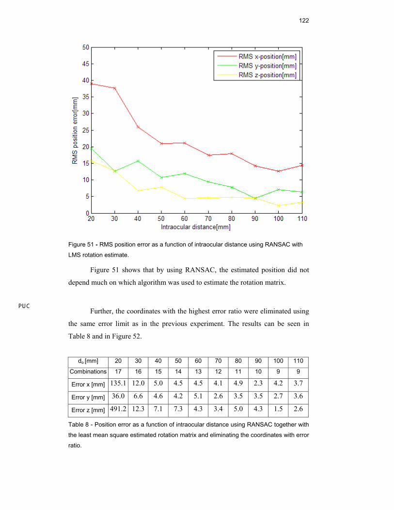
122
Figure 51 - RMS position error as a function of intraocular distance using RANSAC with
LMS rotation estimate.
Figure 51 shows that by using RANSAC, the estimated position did not
depend much on which algorithm was used to estimate the rotation matrix.
Further, the coordinates with the highest error ratio were eliminated using
the same error limit as in the previous experiment. The results can be seen in
Table 8 and in Figure 52.
Table 8 - Position error as a function of intraocular distance using RANSAC together with
the least mean square estimated rotation matrix and eliminating the coordinates with error
ratio.
do [mm] 20 30 40 50 60 70 80 90 100 110
Combinations 17 16 15 14 13 12 11 10 9 9
Error x [mm] 135.1 12.0 5.0 4.5 4.5 4.1 4.9 2.3 4.2 3.7
Error y [mm] 36.0 6.6 4.6 4.2 5.1 2.6 3.5 3.5 2.7 3.6
Error z [mm] 491.2 12.3 7.1 7.3 4.3 3.4 5.0 4.3 1.5 2.6
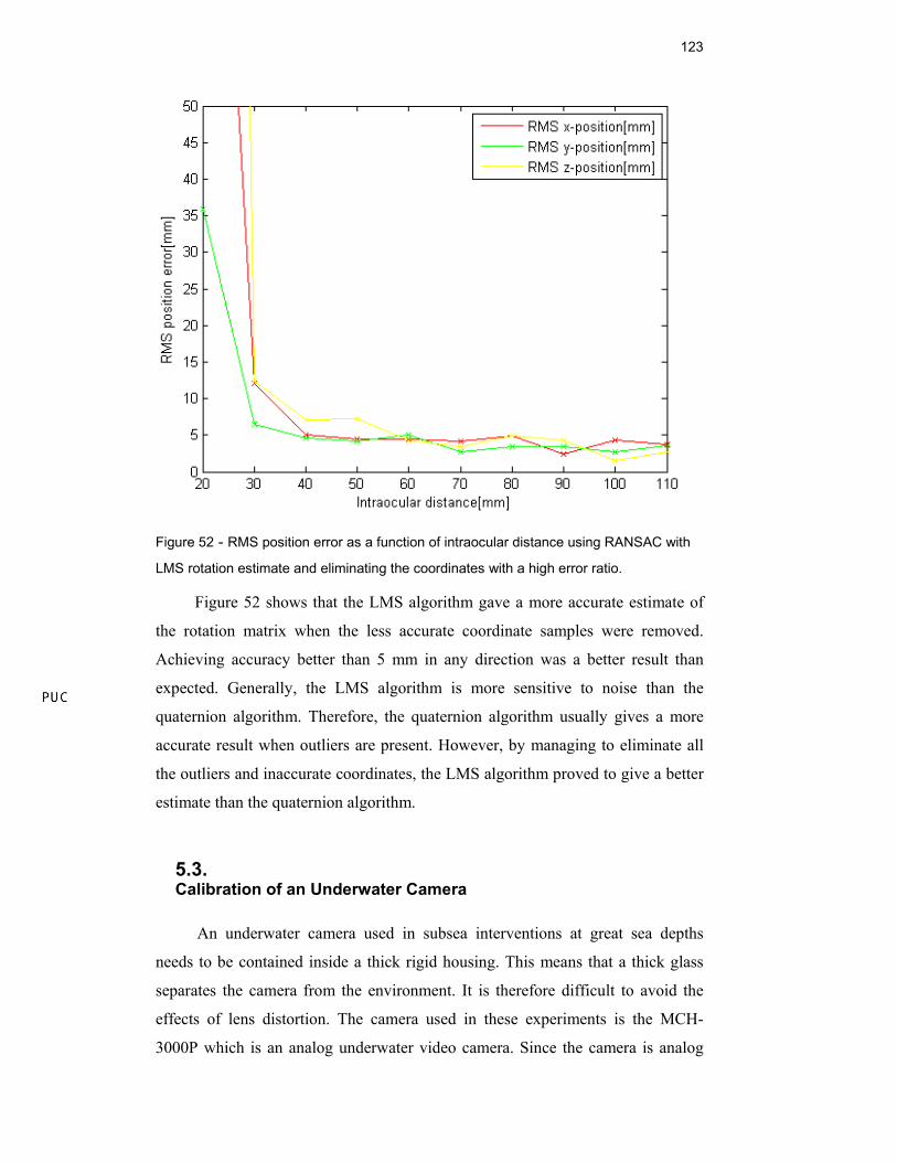
123
Figure 52 - RMS position error as a function of intraocular distance using RANSAC with
LMS rotation estimate and eliminating the coordinates with a high error ratio.
Figure 52 shows that the LMS algorithm gave a more accurate estimate of
the rotation matrix when the less accurate coordinate samples were removed.
Achieving accuracy better than 5 mm in any direction was a better result than
expected. Generally, the LMS algorithm is more sensitive to noise than the
quaternion algorithm. Therefore, the quaternion algorithm usually gives a more
accurate result when outliers are present. However, by managing to eliminate all
the outliers and inaccurate coordinates, the LMS algorithm proved to give a better
estimate than the quaternion algorithm.
5.3. Calibration of an Underwater Camera
An underwater camera used in subsea interventions at great sea depths
needs to be contained inside a thick rigid housing. This means that a thick glass
separates the camera from the environment. It is therefore difficult to avoid the
effects of lens distortion. The camera used in these experiments is the MCH-
3000P which is an analog underwater video camera. Since the camera is analog
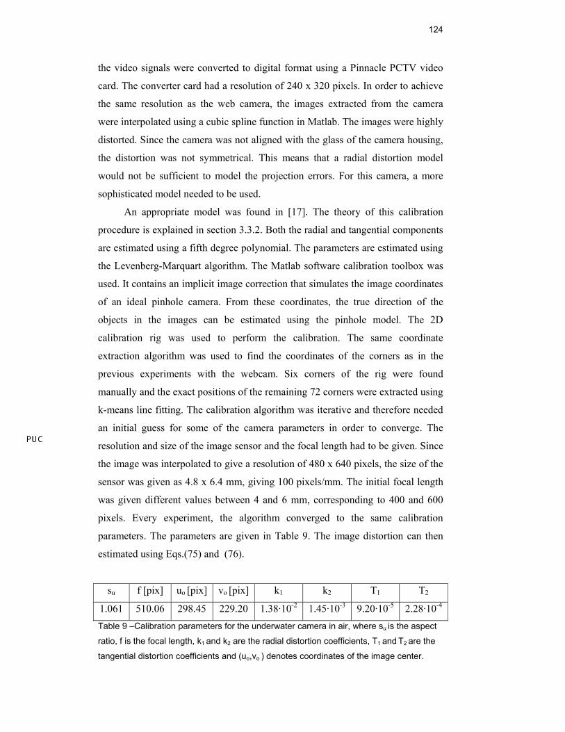
124
the video signals were converted to digital format using a Pinnacle PCTV video
card. The converter card had a resolution of 240 x 320 pixels. In order to achieve
the same resolution as the web camera, the images extracted from the camera
were interpolated using a cubic spline function in Matlab. The images were highly
distorted. Since the camera was not aligned with the glass of the camera housing,
the distortion was not symmetrical. This means that a radial distortion model
would not be sufficient to model the projection errors. For this camera, a more
sophisticated model needed to be used.
An appropriate model was found in [17]. The theory of this calibration
procedure is explained in section 3.3.2. Both the radial and tangential components
are estimated using a fifth degree polynomial. The parameters are estimated using
the Levenberg-Marquart algorithm. The Matlab software calibration toolbox was
used. It contains an implicit image correction that simulates the image coordinates
of an ideal pinhole camera. From these coordinates, the true direction of the
objects in the images can be estimated using the pinhole model. The 2D
calibration rig was used to perform the calibration. The same coordinate
extraction algorithm was used to find the coordinates of the corners as in the
previous experiments with the webcam. Six corners of the rig were found
manually and the exact positions of the remaining 72 corners were extracted using
k-means line fitting. The calibration algorithm was iterative and therefore needed
an initial guess for some of the camera parameters in order to converge. The
resolution and size of the image sensor and the focal length had to be given. Since
the image was interpolated to give a resolution of 480 x 640 pixels, the size of the
sensor was given as 4.8 x 6.4 mm, giving 100 pixels/mm. The initial focal length
was given different values between 4 and 6 mm, corresponding to 400 and 600
pixels. Every experiment, the algorithm converged to the same calibration
parameters. The parameters are given in Table 9. The image distortion can then
estimated using Eqs.(75) and (76).
su f [pix] uo [pix] vo [pix] k1 k2 T1 T2
1.061 510.06 298.45 229.20 1.38·10-2 1.45·10-3 9.20·10-5 2.28·10-4 Table 9 –Calibration parameters for the underwater camera in air, where su is the aspect
ratio, f is the focal length, k1 and k2 are the radial distortion coefficients, T1 and T2 are the
tangential distortion coefficients and (uo,vo ) denotes coordinates of the image center.
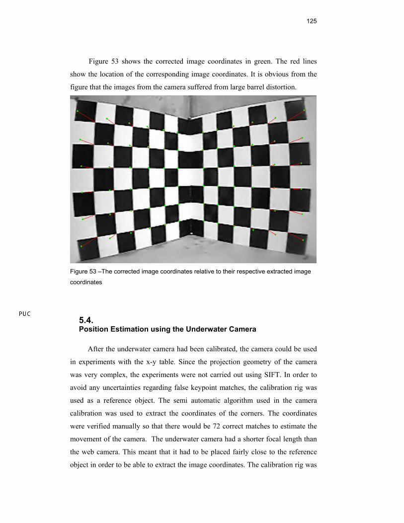
125
Figure 53 shows the corrected image coordinates in green. The red lines
show the location of the corresponding image coordinates. It is obvious from the
figure that the images from the camera suffered from large barrel distortion.
Figure 53 –The corrected image coordinates relative to their respective extracted image
coordinates
5.4. Position Estimation using the Underwater Camera
After the underwater camera had been calibrated, the camera could be used
in experiments with the x-y table. Since the projection geometry of the camera
was very complex, the experiments were not carried out using SIFT. In order to
avoid any uncertainties regarding false keypoint matches, the calibration rig was
used as a reference object. The semi automatic algorithm used in the camera
calibration was used to extract the coordinates of the corners. The coordinates
were verified manually so that there would be 72 correct matches to estimate the
movement of the camera. The underwater camera had a shorter focal length than
the web camera. This meant that it had to be placed fairly close to the reference
object in order to be able to extract the image coordinates. The calibration rig was
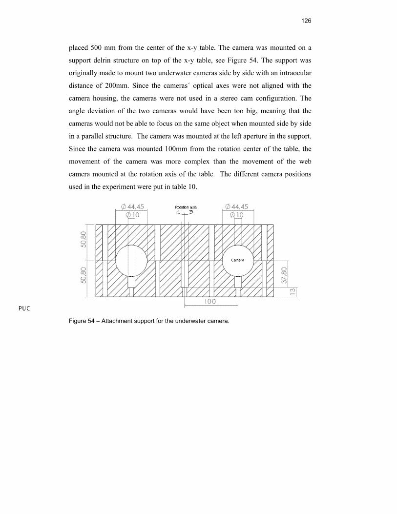
126
placed 500 mm from the center of the x-y table. The camera was mounted on a
support delrin structure on top of the x-y table, see Figure 54. The support was
originally made to mount two underwater cameras side by side with an intraocular
distance of 200mm. Since the cameras´ optical axes were not aligned with the
camera housing, the cameras were not used in a stereo cam configuration. The
angle deviation of the two cameras would have been too big, meaning that the
cameras would not be able to focus on the same object when mounted side by side
in a parallel structure. The camera was mounted at the left aperture in the support.
Since the camera was mounted 100mm from the rotation center of the table, the
movement of the camera was more complex than the movement of the web
camera mounted at the rotation axis of the table. The different camera positions
used in the experiment were put in table 10.
Figure 54 – Attachment support for the underwater camera.
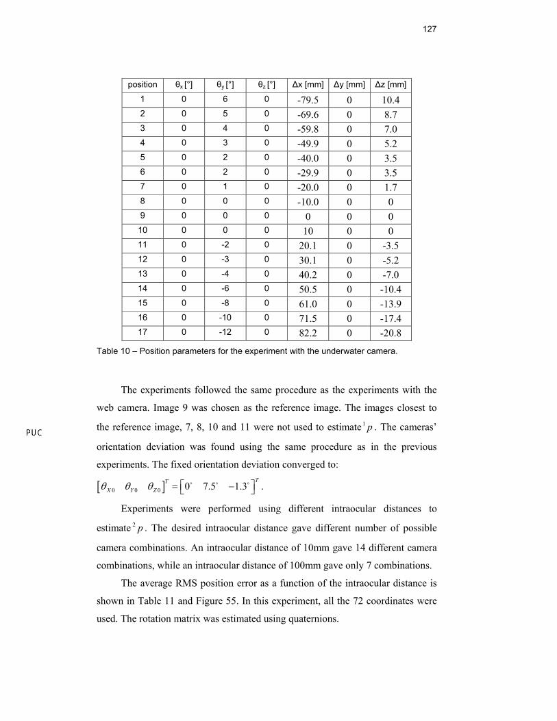
127
position θx [°] θy [°] θz [°] ∆x [mm] ∆y [mm] ∆z [mm]
1 0 6 0 -79.5 0 10.4 2 0 5 0 -69.6 0 8.7 3 0 4 0 -59.8 0 7.0 4 0 3 0 -49.9 0 5.2 5 0 2 0 -40.0 0 3.5 6 0 2 0 -29.9 0 3.5 7 0 1 0 -20.0 0 1.7 8 0 0 0 -10.0 0 0 9 0 0 0 0 0 0 10 0 0 0 10 0 0 11 0 -2 0 20.1 0 -3.5 12 0 -3 0 30.1 0 -5.2 13 0 -4 0 40.2 0 -7.0 14 0 -6 0 50.5 0 -10.4 15 0 -8 0 61.0 0 -13.9 16 0 -10 0 71.5 0 -17.4 17 0 -12 0 82.2 0 -20.8
Table 10 – Position parameters for the experiment with the underwater camera.
The experiments followed the same procedure as the experiments with the
web camera. Image 9 was chosen as the reference image. The images closest to
the reference image, 7, 8, 10 and 11 were not used to estimate p1 . The cameras’
orientation deviation was found using the same procedure as in the previous
experiments. The fixed orientation deviation converged to:
[ ]0 0 0 0 7.5 1.3TT
X Y Zθ θ θ ⎡ ⎤= −⎣ ⎦ .
Experiments were performed using different intraocular distances to
estimate p2 . The desired intraocular distance gave different number of possible
camera combinations. An intraocular distance of 10mm gave 14 different camera
combinations, while an intraocular distance of 100mm gave only 7 combinations.
The average RMS position error as a function of the intraocular distance is
shown in Table 11 and Figure 55. In this experiment, all the 72 coordinates were
used. The rotation matrix was estimated using quaternions.
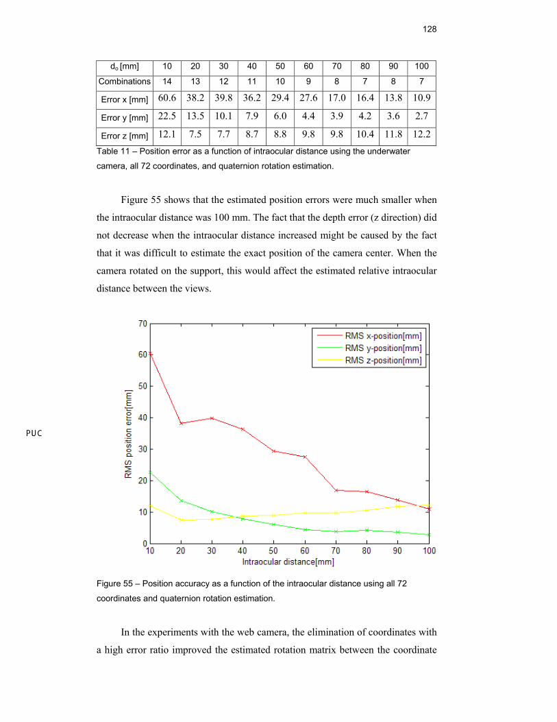
128
Table 11 – Position error as a function of intraocular distance using the underwater
camera, all 72 coordinates, and quaternion rotation estimation.
Figure 55 shows that the estimated position errors were much smaller when
the intraocular distance was 100 mm. The fact that the depth error (z direction) did
not decrease when the intraocular distance increased might be caused by the fact
that it was difficult to estimate the exact position of the camera center. When the
camera rotated on the support, this would affect the estimated relative intraocular
distance between the views.
Figure 55 – Position accuracy as a function of the intraocular distance using all 72
coordinates and quaternion rotation estimation.
In the experiments with the web camera, the elimination of coordinates with
a high error ratio improved the estimated rotation matrix between the coordinate
do [mm] 10 20 30 40 50 60 70 80 90 100
Combinations 14 13 12 11 10 9 8 7 8 7
Error x [mm] 60.6 38.2 39.8 36.2 29.4 27.6 17.0 16.4 13.8 10.9
Error y [mm] 22.5 13.5 10.1 7.9 6.0 4.4 3.9 4.2 3.6 2.7
Error z [mm] 12.1 7.5 7.7 8.7 8.8 9.8 9.8 10.4 11.8 12.2
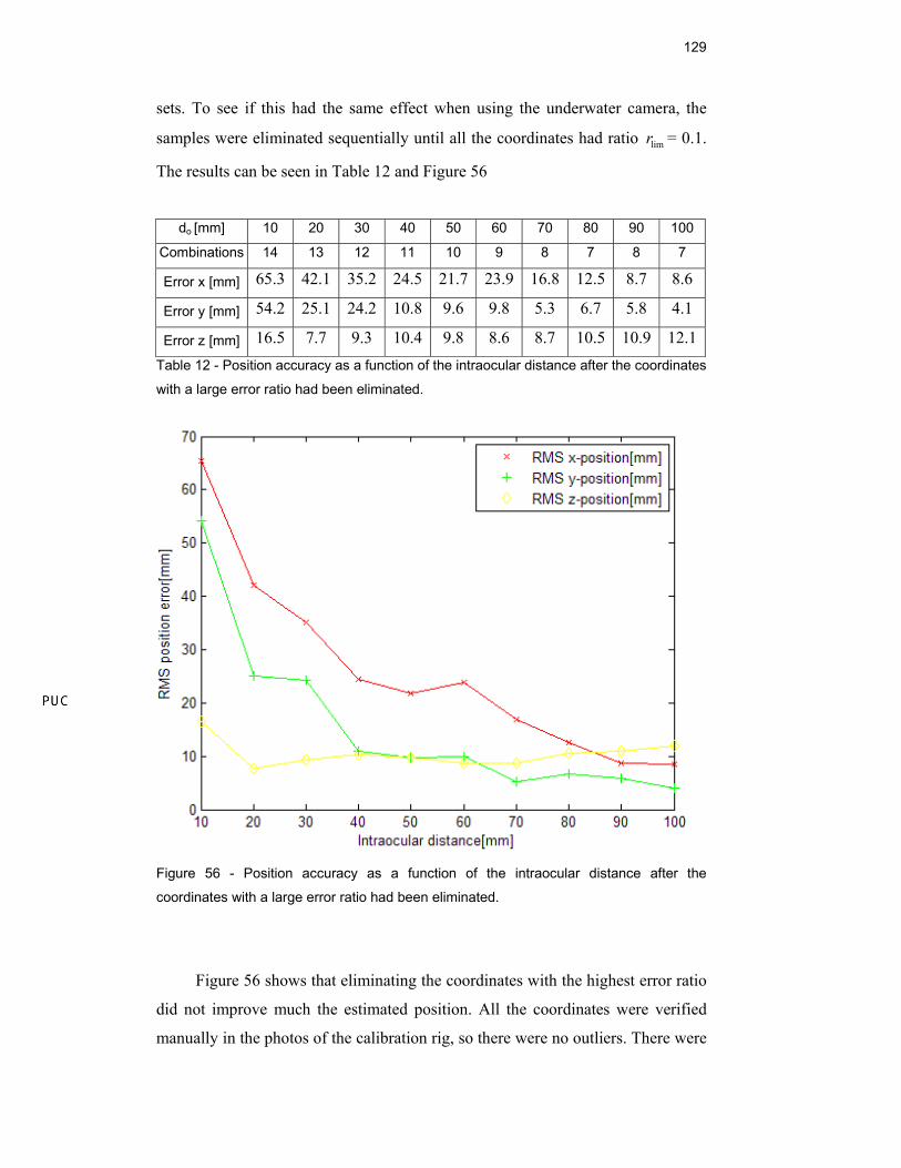
129
sets. To see if this had the same effect when using the underwater camera, the
samples were eliminated sequentially until all the coordinates had ratio limr = 0.1.
The results can be seen in Table 12 and Figure 56
Table 12 - Position accuracy as a function of the intraocular distance after the coordinates
with a large error ratio had been eliminated.
Figure 56 - Position accuracy as a function of the intraocular distance after the
coordinates with a large error ratio had been eliminated.
Figure 56 shows that eliminating the coordinates with the highest error ratio
did not improve much the estimated position. All the coordinates were verified
manually in the photos of the calibration rig, so there were no outliers. There were
do [mm] 10 20 30 40 50 60 70 80 90 100
Combinations 14 13 12 11 10 9 8 7 8 7
Error x [mm] 65.3 42.1 35.2 24.5 21.7 23.9 16.8 12.5 8.7 8.6
Error y [mm] 54.2 25.1 24.2 10.8 9.6 9.8 5.3 6.7 5.8 4.1
Error z [mm] 16.5 7.7 9.3 10.4 9.8 8.6 8.7 10.5 10.9 12.1
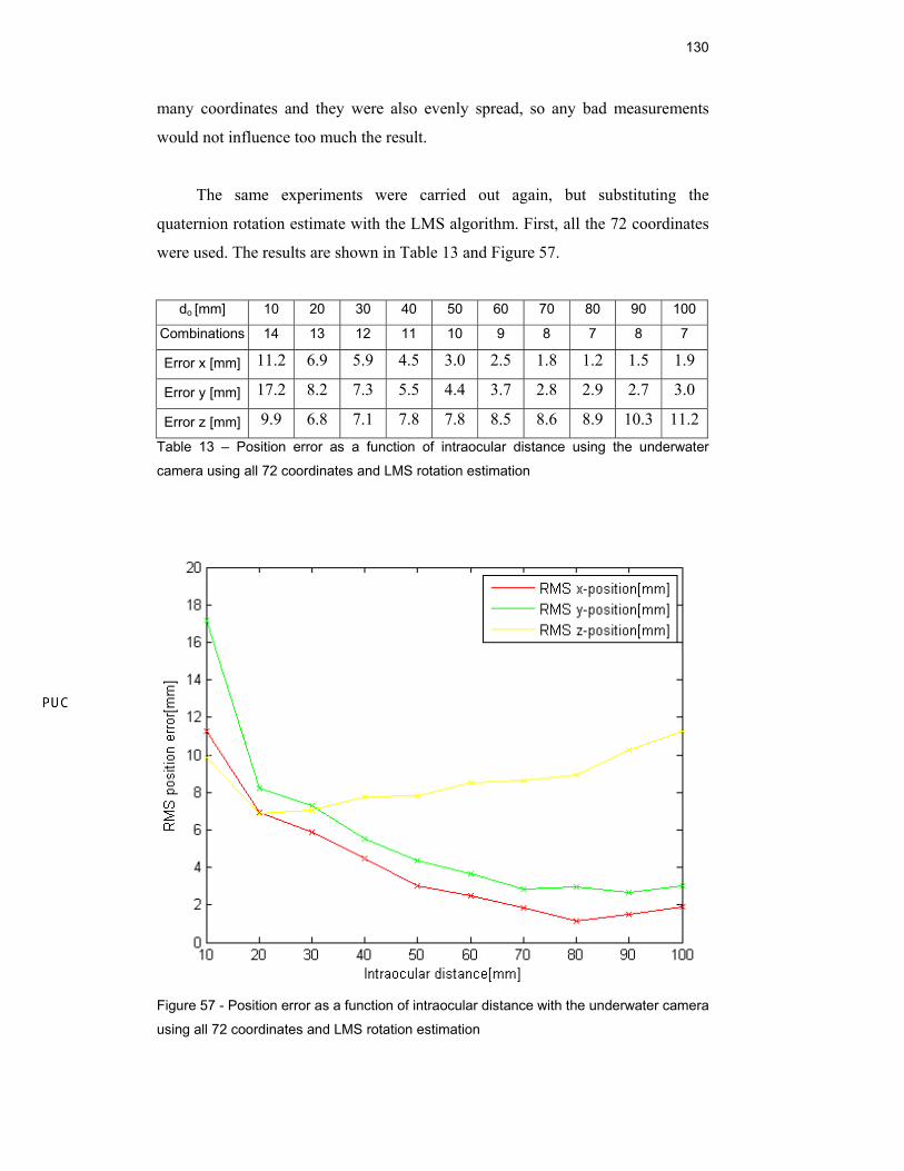
130
many coordinates and they were also evenly spread, so any bad measurements
would not influence too much the result.
The same experiments were carried out again, but substituting the
quaternion rotation estimate with the LMS algorithm. First, all the 72 coordinates
were used. The results are shown in Table 13 and Figure 57.
Table 13 – Position error as a function of intraocular distance using the underwater
camera using all 72 coordinates and LMS rotation estimation
Figure 57 - Position error as a function of intraocular distance with the underwater camera
using all 72 coordinates and LMS rotation estimation
do [mm] 10 20 30 40 50 60 70 80 90 100
Combinations 14 13 12 11 10 9 8 7 8 7
Error x [mm] 11.2 6.9 5.9 4.5 3.0 2.5 1.8 1.2 1.5 1.9
Error y [mm] 17.2 8.2 7.3 5.5 4.4 3.7 2.8 2.9 2.7 3.0
Error z [mm] 9.9 6.8 7.1 7.8 7.8 8.5 8.6 8.9 10.3 11.2
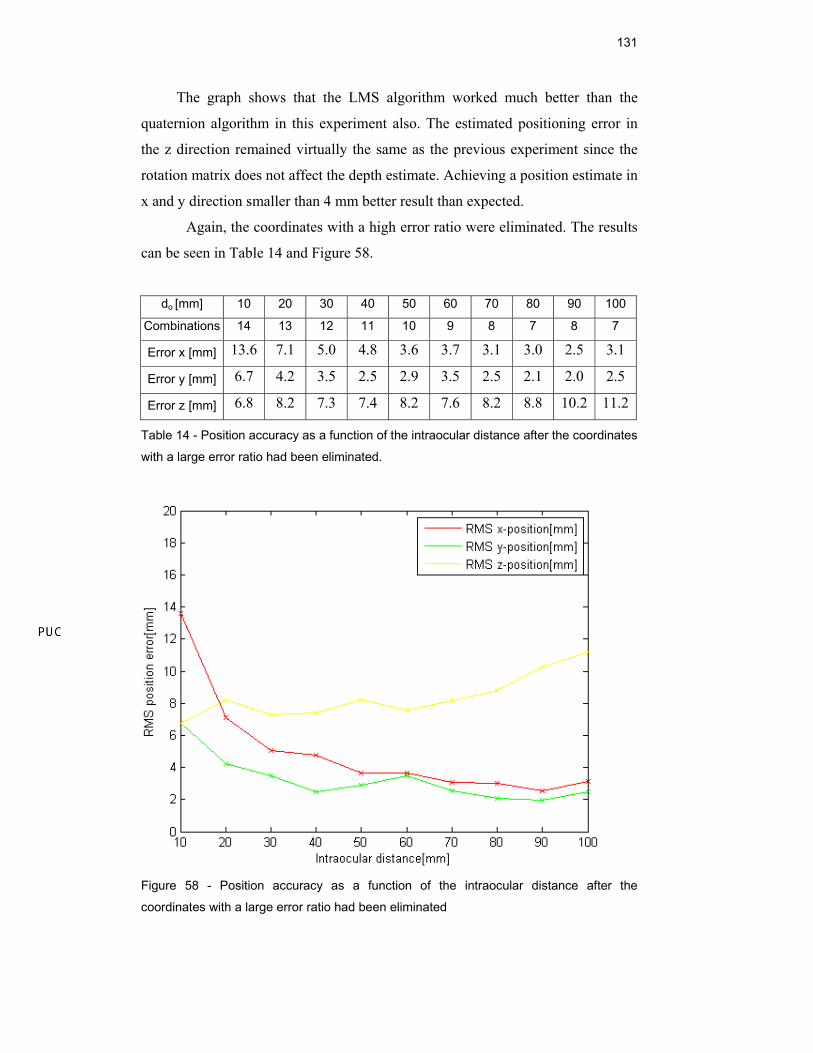
131
The graph shows that the LMS algorithm worked much better than the
quaternion algorithm in this experiment also. The estimated positioning error in
the z direction remained virtually the same as the previous experiment since the
rotation matrix does not affect the depth estimate. Achieving a position estimate in
x and y direction smaller than 4 mm better result than expected.
Again, the coordinates with a high error ratio were eliminated. The results
can be seen in Table 14 and Figure 58.
Table 14 - Position accuracy as a function of the intraocular distance after the coordinates
with a large error ratio had been eliminated.
Figure 58 - Position accuracy as a function of the intraocular distance after the
coordinates with a large error ratio had been eliminated
do [mm] 10 20 30 40 50 60 70 80 90 100
Combinations 14 13 12 11 10 9 8 7 8 7
Error x [mm] 13.6 7.1 5.0 4.8 3.6 3.7 3.1 3.0 2.5 3.1
Error y [mm] 6.7 4.2 3.5 2.5 2.9 3.5 2.5 2.1 2.0 2.5
Error z [mm] 6.8 8.2 7.3 7.4 8.2 7.6 8.2 8.8 10.2 11.2
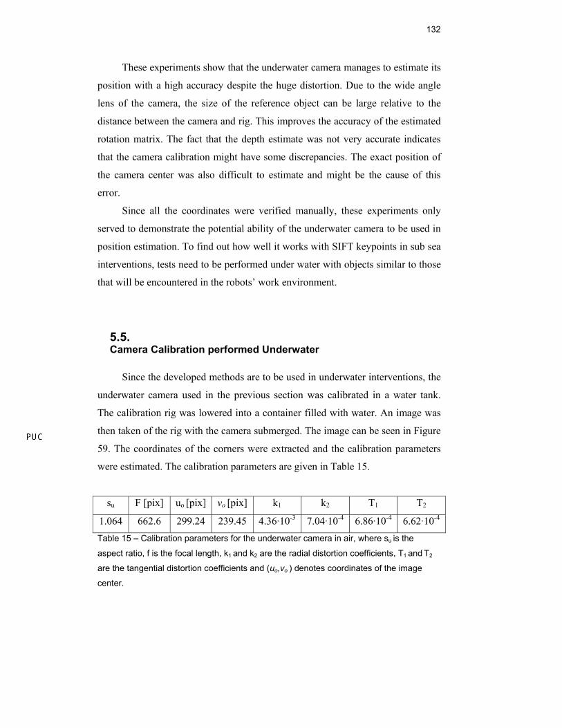
132
These experiments show that the underwater camera manages to estimate its
position with a high accuracy despite the huge distortion. Due to the wide angle
lens of the camera, the size of the reference object can be large relative to the
distance between the camera and rig. This improves the accuracy of the estimated
rotation matrix. The fact that the depth estimate was not very accurate indicates
that the camera calibration might have some discrepancies. The exact position of
the camera center was also difficult to estimate and might be the cause of this
error.
Since all the coordinates were verified manually, these experiments only
served to demonstrate the potential ability of the underwater camera to be used in
position estimation. To find out how well it works with SIFT keypoints in sub sea
interventions, tests need to be performed under water with objects similar to those
that will be encountered in the robots’ work environment.
5.5. Camera Calibration performed Underwater
Since the developed methods are to be used in underwater interventions, the
underwater camera used in the previous section was calibrated in a water tank.
The calibration rig was lowered into a container filled with water. An image was
then taken of the rig with the camera submerged. The image can be seen in Figure
59. The coordinates of the corners were extracted and the calibration parameters
were estimated. The calibration parameters are given in Table 15.
su F [pix] uo [pix] vo [pix] k1 k2 T1 T2
1.064 662.6 299.24 239.45 4.36·10-3 7.04·10-4 6.86·10-4 6.62·10-4 Table 15 – Calibration parameters for the underwater camera in air, where su is the
aspect ratio, f is the focal length, k1 and k2 are the radial distortion coefficients, T1 and T2
are the tangential distortion coefficients and (uo,vo ) denotes coordinates of the image
center.
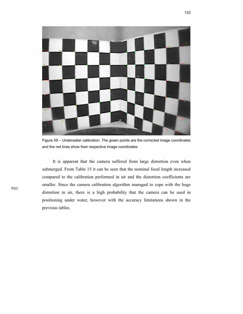
133
Figure 59 – Underwater calibration. The green points are the corrected image coordinates
and the red lines show their respective image coordinates
It is apparent that the camera suffered from large distortion even when
submerged. From Table 15 it can be seen that the nominal focal length increased
compared to the calibration performed in air and the distortion coefficients are
smaller. Since the camera calibration algorithm managed to cope with the huge
distortion in air, there is a high probability that the camera can be used in
positioning under water, however with the accuracy limitations shown in the
previous tables.
6 Conclusions and Suggestions
6.1. Conclusions
This work has contributed to elaborate a general technique that enables a
robot to calculate its position relative to the environment through the use of a
camera. The method has proven to achieve a fair accuracy in the experiments
performed. The techniques used in this work are not specific for the TA-40
manipulator and can be applied to any manipulator.
Incorporating both calibration of the manipulator structure as well as the
calibration of the manipulator base, this work includes the initial steps required to
achieve a good absolute precision in the work environment. This can be used to
give feedback to the operator in a virtual environment. In this virtual environment,
work procedures and trajectories could be planned and programmed without the
use of the manipulator.
When the manipulator has attained a good absolute precision and the
absolute position of the base has been estimated, the inverse kinematic model
could be used to perform preprogrammed trajectories. In this way, many of the
operators’ tasks could be automated.
All the kinematic models for the TA-40 manipulator have been developed.
Experiments were performed using an x-y table and two cameras; a webcam and
an underwater camera. The webcam achieved to estimate its position with an error
less than 5mm RMS in all directions. The underwater camera achieved an
accuracy of approximately 10mm RMS. The LMS algorithm gave the most
accurate estimate of the relative orientation between two views and hence gave a
more accurate position for both cameras.
135
6.2. Suggestions for future work
During this project methods have been developed that allow a manipulator
to estimate its relative position in a 3D environment. The method uses the SIFT
algorithm which is a fairly new algorithm in computer vision. This work has used
a Matlab implementation of the algorithm in the experiments. The algorithm is
computationally heavy. In Matlab, estimating the SIFT keypoints for one image
may take several minutes. When working in the laboratory this is not such big
problem, but when the manipulator is to perform a real time base calibration, the
process needs to be sped up. SIFT is subject for a lot of research, so some
improvements to the algorithm can be expected.
In [25] several different region detectors were used to detect interest areas
for the SIFT algorithm. The different region detectors proved to find the most
likely areas to find robust keypoints, meaning that SIFT did not have to be
computed on the whole image, making the computation faster.
When it comes to the use of underwater cameras in position estimation,
there are a few problem areas that need to be solved. Due to the thick glass in
front of the camera, the images will suffer from distortion. When the distortion is
large, it might influence the recognition of SIFT keypoints. To investigate the
potential use of the underwater camera in positioning, underwater tests need to be
performed using objects of interest that are similar to the ones found in the
manipulator’s actual work environment. The resolution of the digital converter
board should also be able to make use of the full resolution of the analog camera.
It would also be advantageous if the images could be stored in a format without
compression to avoid any distortion that a compressed image might have.
7 References
[1] Meggiolaro, M., Jaffe, P.C.L., Dubowsky, S., “Achieving Fine Absolute
Positioning Accuracy in Large Powerful Manipulators”, Anais do
International Conference on Robotics and Automation (ICRA '99), IEEE,
Detroit, Michigan, USA, pp.2819-2824, 1999a.
[2] Meggiolaro, M., Dubowsky, S., “An Analytical Method to Eliminate the
Redundant Parameters in Robot Calibration”, Anais do International
Conference on Robotics and Automation (ICRA '2000), IEEE, San
Francisco, CA, USA, pp. 3609-3615, 2000a.
[3] David G. Lowe, "Distinctive Image Features from Scale-Invariant
Keypoints", The International Journal of Computer Vision, 2004.
[4] Denavit. J.; R. S. Hartenberg., “A Kinematic Notation for Lower-Pair
Mechanisms Based on Matrices”, ASME J. Applied Mechanics. pp.215-221.
1955.
[5] Asada. H. and Slotine, "Robot Analysis and Control", Wiley. New York.
1986.
[6] Meggiolaro. M.,”Achieving Fine Absolute Positioning Accuracy
in Large Powerful Manipulators”, PhD thesis. Department of Mechanical
Engineering. Massachusets Institute of Technology. Massachusetts. 2000a
[7] Zhuang. H.. Motaghedi. S.H.. Roth. Z.S.. “Robot Calibration with Planar
Constraints”. Proc. IEEE International Conference of Robotics and
Automation. Detroit. Michigan. pp.805-810. 1999.
137
[8] Marques G.C., “Calibração Remota de Sistemas Robóticos Utilizando
Sensores Internos e Externos”, UFRJ 2005.
[9] Hollerbach. J.M.. Wampler. C.W., “The Calibration Index and Taxonomy for
Robot Kinematic Calibration Methods”, International Journal of Robotics
Research. Vol. 15. No. 6. pp. 573-591. 1996.
[10] Pieper. D.L.. “The kinematics of manipulators under computer control”,
Stanford Artificial Intelligence Laboratory. Stanford University. AIM 72.
1968.
[11] Bernard R. , “Robot Calibration” , Kluwer 1993.
[12] Leica laser tracker manual, 2006.
[13] A.B. Forbes., “Least-square best-fit geometric elements NPL Report DITC
140/89”
[14] Feitosa R.Q., “Lecture slides”, Puc-Rio, 2006
[15] Forsyth. D. A.; Ponce J., “Computer Vision. a Modern Approach”, ed.
Prentice Hall. 2003
[16] “A Flexible New Technique for Camera Calibration”, Zhengyou Zhang,
March 1999,
[17] Heikkilä J., Silvén O., “A Four-step Camera Calibration Procedure with
Implicit Image Correction”, In Proceedings of Computer Vision and
Pattern Recognition (CVPR), page 1106, Washington, DC, USA, 1997.
IEEE Computer Society.
[18] David G. Lowe, "Object Recognition from Local Scale-Invariant Features",
1999.
138
[19] Fischler M. A.; Bolles R. C., “Random Sample Consensus; A paradigm for
Model Fitting with Applications to Image Analysis and Automated
Cartography”. Comm. Of the ACM. Vol 24. pp. 381-395. 1981
[20] Ballard, D. R, "Generalizing the Hough Transform to Detect. Arbitrary
Shapes”, Pattern Recognition, Vol. 13, No. 2, 1981,. pp. 111-122.
[21] Chaudhuri, S. Chatterjee, S, “On analyzing the performance of least squares
methods in motion estimation” , University of California. 1989
[22] Zhuang. Hanqi; Roth. S. Zvi, “Camera-Aided Robot Calibration”. ed. CRC
Press. Inc. 1996
[23] TA-40 manual, Petrobras.
[24] Pinto M.A.G.,” Pocisionamento e Calibração de um Manipulador Robotico
Submarino com Uso de Visão Computacional”, Puc-Rio, 2006
[25] K. Mikolajczyk, T. Tuytelaars, C. Schmid, A. Zisserman, J. Matas, F.
Schaffalitzky, T. Kadir and L. Van Gool, A comparison of affine region
detectors. In International Journal of Computer Vision 65(1/2):43-72, 2005
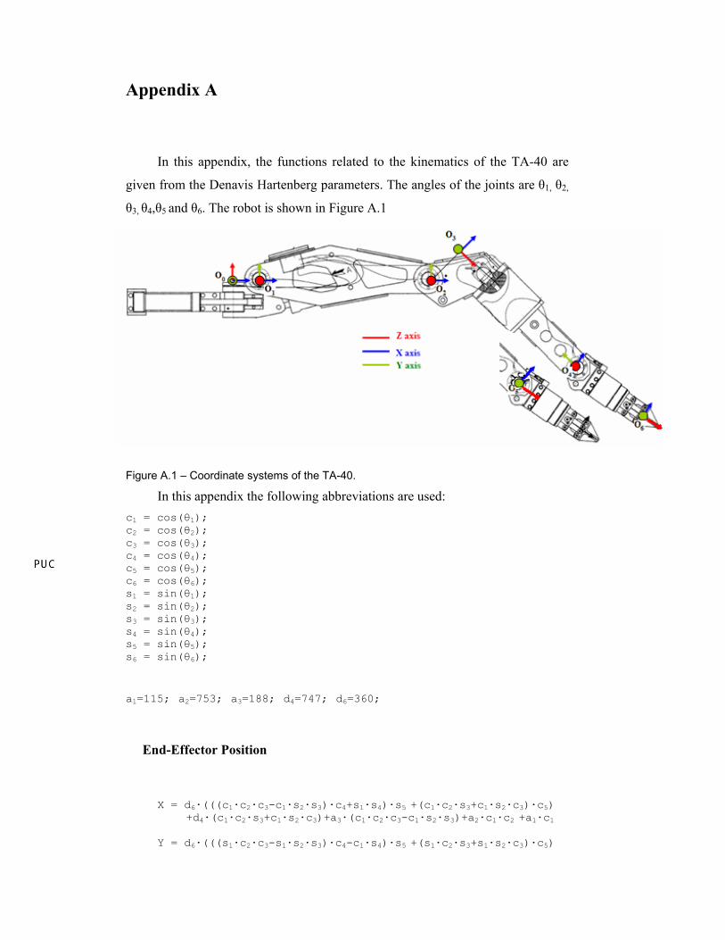
Appendix A
In this appendix, the functions related to the kinematics of the TA-40 are
given from the Denavis Hartenberg parameters. The angles of the joints are θ1, θ2,
θ3, θ4,θ5 and θ6. The robot is shown in Figure A.1
Figure A.1 – Coordinate systems of the TA-40.
In this appendix the following abbreviations are used: c1 = cos(θ1); c2 = cos(θ2); c3 = cos(θ3); c4 = cos(θ4); c5 = cos(θ5); c6 = cos(θ6); s1 = sin(θ1); s2 = sin(θ2); s3 = sin(θ3); s4 = sin(θ4); s5 = sin(θ5); s6 = sin(θ6);
a1=115; a2=753; a3=188; d4=747; d6=360;
End-Effector Position
X = d6·(((c1·c2·c3-c1·s2·s3)·c4+s1·s4)·s5 +(c1·c2·s3+c1·s2·c3)·c5) +d4·(c1·c2·s3+c1·s2·c3)+a3·(c1·c2·c3-c1·s2·s3)+a2·c1·c2 +a1·c1
Y = d6·(((s1·c2·c3-s1·s2·s3)·c4-c1·s4)·s5 +(s1·c2·s3+s1·s2·c3)·c5)
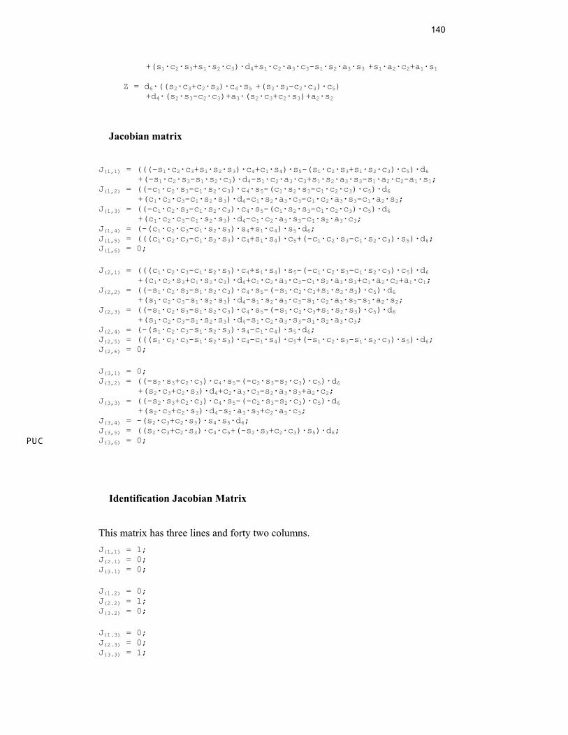
140
+(s1·c2·s3+s1·s2·c3)·d4+s1·c2·a3·c3-s1·s2·a3·s3 +s1·a2·c2+a1·s1 Z = d6·((s2·c3+c2·s3)·c4·s5 +(s2·s3-c2·c3)·c5) +d4·(s2·s3-c2·c3)+a3·(s2·c3+c2·s3)+a2·s2
Jacobian matrix
J(1,1) = (((-s1·c2·c3+s1·s2·s3)·c4+c1·s4)·s5-(s1·c2·s3+s1·s2·c3)·c5)·d6 +(-s1·c2·s3-s1·s2·c3)·d4-s1·c2·a3·c3+s1·s2·a3·s3-s1·a2·c2-a1·s1;
J(1,2) = ((-c1·c2·s3-c1·s2·c3)·c4·s5-(c1·s2·s3-c1·c2·c3)·c5)·d6 +(c1·c2·c3-c1·s2·s3)·d4-c1·s2·a3·c3-c1·c2·a3·s3-c1·a2·s2;
J(1,3) = ((-c1·c2·s3-c1·s2·c3)·c4·s5-(c1·s2·s3-c1·c2·c3)·c5)·d6 +(c1·c2·c3-c1·s2·s3)·d4-c1·c2·a3·s3-c1·s2·a3·c3;
J(1,4) = (-(c1·c2·c3-c1·s2·s3)·s4+s1·c4)·s5·d6; J(1,5) = (((c1·c2·c3-c1·s2·s3)·c4+s1·s4)·c5+(-c1·c2·s3-c1·s2·c3)·s5)·d6; J(1,6) = 0; J(2,1) = (((c1·c2·c3-c1·s2·s3)·c4+s1·s4)·s5-(-c1·c2·s3-c1·s2·c3)·c5)·d6
+(c1·c2·s3+c1·s2·c3)·d4+c1·c2·a3·c3-c1·s2·a3·s3+c1·a2·c2+a1·c1; J(2,2) = ((-s1·c2·s3-s1·s2·c3)·c4·s5-(-s1·c2·c3+s1·s2·s3)·c5)·d6
+(s1·c2·c3-s1·s2·s3)·d4-s1·s2·a3·c3-s1·c2·a3·s3-s1·a2·s2; J(2,3) = ((-s1·c2·s3-s1·s2·c3)·c4·s5-(-s1·c2·c3+s1·s2·s3)·c5)·d6
+(s1·c2·c3-s1·s2·s3)·d4-s1·c2·a3·s3-s1·s2·a3·c3; J(2,4) = (-(s1·c2·c3-s1·s2·s3)·s4-c1·c4)·s5·d6; J(2,5) = (((s1·c2·c3-s1·s2·s3)·c4-c1·s4)·c5+(-s1·c2·s3-s1·s2·c3)·s5)·d6; J(2,6) = 0; J(3,1) = 0; J(3,2) = ((-s2·s3+c2·c3)·c4·s5-(-c2·s3-s2·c3)·c5)·d6
+(s2·c3+c2·s3)·d4+c2·a3·c3-s2·a3·s3+a2·c2; J(3,3) = ((-s2·s3+c2·c3)·c4·s5-(-c2·s3-s2·c3)·c5)·d6
+(s2·c3+c2·s3)·d4-s2·a3·s3+c2·a3·c3; J(3,4) = -(s2·c3+c2·s3)·s4·s5·d6; J(3,5) = ((s2·c3+c2·s3)·c4·c5+(-s2·s3+c2·c3)·s5)·d6; J(3,6) = 0;
Identification Jacobian Matrix
This matrix has three lines and forty two columns. J(1,1) = 1; J(2.1) = 0; J(3.1) = 0; J(1.2) = 0; J(2.2) = 1; J(3.2) = 0; J(1.3) = 0; J(2.3) = 0; J(3.3) = 1;
141
J(1.4) = s2·a3·c3+a2·s2+c2·a3·s3+(s2·s3-c2·c3)·d4 +((s2·c3+c2·s3)·c4·s5-(-s2·s3+c2·c3)·c5)·d6;
J(2.4) = 0; J(3.4) = c1·s2·a3·s3-a1·c1-c1·a2·c2-c1·c2·a3·c3+(-c1·c2·s3-c1·s2·c3)·d4
+(((-c1·c2·c3+c1·s2·s3)·c4-s1·s4)·s5-(c1·c2·s3+c1·s2·c3)·c5)·d6; J(1.5) = -s1·c2·a3·c3+s1·s2·a3·s3-a1·s1-s1·a2·c2+(-s1·c2·s3-s1·s2·c3)·d4
+(((-s1·c2·c3+s1·s2·s3)·c4+c1·s4)·s5-(s1·c2·s3+s1·s2·c3)·c5)·d6; J(2.5) = c1·c2·a3·c3-c1·s2·a3·s3+a1·c1+c1·a2·c2 +(c1·c2·s3+c1·s2·c3)·d4
+(((c1·c2·c3-c1·s2·s3)·c4+s1·s4)·s5+(c1·c2·s3+c1·s2·c3)·c5)·d6; J(3.5) = 0; J(1.6) = 0; J(2.6) = -a2·s2-s2·a3·c3-c2·a3·s3+(-s2·s3+c2·c3)·d4
+((-s2·c3-c2·s3)·c4·s5-(s2·s3-c2·c3)·c5)·d6; J(3.6) = a1·s1-s1·s2·a3·s3+s1·a2·c2+s1·c2·a3·c3 +(s1·c2·s3+s1·s2·c3)·d4
+(((s1·c2·c3-s1·s2·s3)·c4-c1·s4)·s5+(s1·c2·s3+s1·s2·c3)·c5)·d6; J(1.7) = c1; J(2.7) = s1; J(3.7) = 0; J(1.8) = 0; J(2.8) = 0; J(3.8) = 1; J(1.9) = s1; J(2.9) = -c1; J(3.9) = 0; J(1.10) = -s1·c2·a3·c3+s1·s2·a3·s3-s1·a2·c2-(s1·c2·s3+s1·s2·c3)·d4
+(((-s1·c2·c3+s1·s2·s3)·c4+c1·s4)·s5-(s1·c2·s3+s1·s2·c3)·c5)·d6; J(2.10) = c1·c2·a3·c3-c1·s2·a3·s3+c1·a2·c2+(c1·c2·s3+c1·s2·c3)·d4
+(((c1·c2·c3-c1·s2·s3)·c4+s1·s4)·s5+(c1·c2·s3+c1·s2·c3)·c5)·d6; J(3.10) = 0; J(1.11) = -c1·s2·a3·c3-c1·a2·s2-c1·c2·a3·s3+(-c1·s2·s3+c1·c2·c3)·d4
+((-c1·s2·c3-c1·c2·s3)·c4·s5-(c1·s2·s3-c1·c2·c3)·c5)·d6; J(2.11) = -s1·a2·s2-s1·s2·a3·c3-s1·c2·a3·s3+(-s1·s2·s3+s1·c2·c3)·d4
+((-s1·s2·c3-s1·c2·s3)·c4·s5-(s1·s2·s3-s1·c2·c3)·c5)·d6; J(3.11) = -s2·a3·s3+a2·c2+c2·a3·c3+(c2·s3+s2·c3)·d4+((c2·c3-s2·s3)·c4·s5
+(c2·s3+s2·c3)·c5)·d6; J(1.12) = s1·s2·a3·c3+s1·a2·s2+s1·c2·a3·s3+(s1·s2·s3-s1·c2·c3)·d4
+((s1·s2·c3+s1·c2·s3)·c4·s5-(-s1·s2·s3+s1·c2·c3)·c5)·d6; J(2.12) = -c1·a2·s2-c1·s2·a3·c3-c1·c2·a3·s3+(-c1·s2·s3+c1·c2·c3)·d4
+((-c1·s2·c3-c1·c2·s3)·c4·s5-(c1·s2·s3-c1·c2·c3)·c5)·d6; J(3.12) = -s4·s5·d6; J(1.13) = c1·c2; J(2.13) = s1·c2; J(3.13) = s2; J(1.14) = -c1·s2; J(2.14) = -s1·s2; J(3.14) = c2; J(1.15) = s1; J(2.15) = -c1;
142
J(3.15) = 0; J(1.16) = -s1·a3·c3-s1·s3·d4+((-s1·c3·c4+c1·c2·s4)·s5-s1·s3·c5)·d6; J(2.16) = c1·a3·c3+c1·s3·d4+((c1·c3·c4+s1·c2·s4)·s5+c1·s3·c5)·d6; J(3.16) = s2·s4·s5·d6; J(1.17) = -c1·s2·a3·c3-c1·c2·a3·s3+(-c1·s2·s3+c1·c2·c3)·d4
+((-c1·s2·c3-c1·c2·s3)·c4·s5-(c1·s2·s3-c1·c2·c3)·c5)·d6;
J(2.17) = -s1·s2·a3·c3-s1·c2·a3·s3+(-s1·s2·s3+s1·c2·c3)·d4 +((-s1·s2·c3-s1·c2·s3)·c4·s5-(s1·s2·s3-s1·c2·c3)·c5)·d6;
J(3.17) = -s2·a3·s3+c2·a3·c3+(c2·s3+s2·c3)·d4+((c2·c3-s2·s3)·c4·s5
+(c2·s3+s2·c3)·c5)·d6; J(1.18) = s1·a3·s3-s1·c3·d4+((s1·s3·c4+c1·s2·s4)·s5-s1·c3·c5)·d6; J(2.18) = -c1·a3·s3+c1·c3·d4+((-c1·s3·c4+s1·s2·s4)·s5+c1·c3·c5)·d6; J(3.18) = -c2·s4·s5·d6; J(1.19) = c1·c2·c3-c1·s2·s3; J(2.19) = s1·c2·c3-s1·s2·s3; J(3.19) = s2·c3+c2·s3; J(1.20) = s1; J(2.20) = -c1; J(3.20) = 0; J(1.21) = c1·c2·s3+c1·s2·c3; J(2.21) = s1·c2·s3+s1·s2·c3; J(3.21) = s2·s3-c2·c3; J(1.22) = (c1·c2·c3-c1·s2·s3)·d4+((-c1·c2·s3-c1·s2·c3)·c4·s5
+(c1·c2·c3-c1·s2·s3)·c5)·d6; J(2.22) = (s1·c2·c3-s1·s2·s3)·d4+((-s1·c2·s3-s1·s2·c3)·c4·s5
+(s1·c2·c3-s1·s2·s3)·c5)·d6; J(3.22) = (s2·c3+c2·s3)·d4+((-s2·s3+c2·c3)·c4·s5+(s2·c3+c2·s3)·c5)·d6; J(1.23) = (s1·c4+(-c1·c2·c3+c1·s2·s3)·s4)·s5·d6; J(2.23) = (-c1·c4+(-s1·c2·c3+s1·s2·s3)·s4)·s5·d6; J(3.23) = (-s2·c3-c2·s3)·s4·s5·d6; J(1.24) = -s1·d4+((c1·c2·s3+c1·s2·c3)·s4·s5-s1·c5)·d6; J(2.24) = c1·d4+((s1·c2·s3+s1·s2·c3)·s4·s5+c1·c5)·d6; J(3.24) = (s2·s3-c2·c3)·s4·s5·d6; J(1.25) = (c1·c2·c3-c1·s2·s3)·c4+s1·s4; J(2.25) = (s1·c2·c3-s1·s2·s3)·c4-c1·s4; J(3.25) = (s2·c3+c2·s3)·c4; J(1.26) = -c1·c2·s3-c1·s2·c3; J(2.26) = -s1·c2·s3-s1·s2·c3; J(3.26) = -s2·s3+c2·c3; J(1.27) = (-c1·c2·c3+c1·s2·s3)·s4+s1·c4; J(2.27) = (-s1·c2·c3+s1·s2·s3)·s4-c1·c4; J(3.27) = (-s2·c3-c2·s3)·s4; J(1.28) = ((c1·c2·c3-c1·s2·s3)·s4-s1·c4)·s5·d6; J(2.28) = ((s1·c2·c3-s1·s2·s3)·s4+c1·c4)·s5·d6;
143
J(3.28) = (s2·c3+c2·s3)·s4·s5·d6; J(1.29) = ((-c1·c2·s3-c1·s2·c3)·s5+((c1·c2·c3-c1·s2·s3)·c4-s1·s4)·c5)·d6; J(2.29) = ((-s1·c2·s3-s1·s2·c3)·s5+((s1·c2·c3-s1·s2·s3)·c4+c1·s4)·c5)·d6; J(3.29) = ((-s2·s3+c2·c3)·s5+(s2·c3+c2·s3)·c4·c5)·d6; J(1.30) = -((-c1·c2·c3+c1·s2·s3)·s4+s1·c4)·c5·d6; J(2.30) = -((-s1·c2·c3+s1·s2·s3)·s4-c1·c4)·c5·d6; J(3.30) = -(-s2·c3-c2·s3)·s4·c5·d6; J(1.31) = ((c1·c2·c3-c1·s2·s3)·c4+s1·s4)·c5-(c1·c2·s3+c1·s2·c3)·s5; J(2.31) = ((s1·c2·c3-s1·s2·s3)·c4-c1·s4)·c5-(s1·c2·s3+s1·s2·c3)·s5; J(3.31) = (s2·c3+c2·s3)·c4·c5+(-s2·s3+c2·c3)·s5; J(1.32) = -(c1·c2·c3-c1·s2·s3)·s4+s1·c4; J(2.32) = -(s1·c2·c3-s1·s2·s3)·s4-c1·c4; J(3.32) = -(s2·c3+c2·s3)·s4; J(1.33) = ((c1·c2·c3-c1·s2·s3)·c4+s1·s4)·s5+(c1·c2·s3+c1·s2·c3)·c5; J(2.33) = ((s1·c2·c3-s1·s2·s3)·c4-c1·s4)·s5+(s1·c2·s3+s1·s2·c3)·c5; J(3.33) = (s2·c3+c2·s3)·c4·s5+(s2·s3-c2·c3)·c5; J(1.34) = (((c1·c2·c3-c1·s2·s3)·c4+s1·s4)·c5-(c1·c2·s3+c1·s2·c3)·s5)·d6; J(2.34) = (((s1·c2·c3-s1·s2·s3)·c4-c1·s4)·c5-(s1·c2·s3+s1·s2·c3)·s5)·d6; J(3.34) = ((s2·c3+c2·s3)·c4·c5+(c2·c3-s2·s3)·s5)·d6; J(1.35) = 0; J(2.35) = 0; J(3.35) = 0; J(1.36) = ((c1·c2·c3-c1·s2·s3)·s4-s1·c4)·d6; J(2.36) = ((s1·c2·c3-s1·s2·s3)·s4+c1·c4)·d6; J(3.36) = (s2·c3+c2·s3)·s4·d6; J(1.37) = (((c1·c2·c3-c1·s2·s3)·c4+s1·s4)·c5-(c1·c2·s3+c1·s2·c3)·s5)·c6
+(-(c1·c2·c3-c1·s2·s3)·s4+s1·c4)·s6; J(2.37) = (((s1·c2·c3-s1·s2·s3)·c4-c1·s4)·c5-(s1·c2·s3+s1·s2·c3)·s5)·c6
+(-(s1·c2·c3-s1·s2·s3)·s4-c1·c4)·s6; J(3.37) = ((s2·c3+c2·s3)·c4·c5+(-s2·s3+c2·c3)·s5)·c6-(s2·c3+c2·s3)·s4·s6; J(1.38) = (-((c1·c2·c3-c1·s2·s3)·c4+s1·s4)·c5
+(c1·c2·s3+c1·s2·c3)·s5)·s6+(-(c1·c2·c3- c1·s2·s3)·s4+s1·c4)·c6; J(2.38) = (-((s1·c2·c3-s1·s2·s3)·c4-c1·s4)·c5+(s1·c2·s3+s1·s2·c3)·s5)·s6
+(-(s1·c2·c3-s1·s2·s3)·s4-c1·c4)·c6; J(3.38) = (-(s2·c3+c2·s3)·c4·c5-(-s2·s3+c2·c3)·s5)·s6-(s2·c3+c2·s3)·s4·c6; J(1.39) = ((c1·c2·c3-c1·s2·s3)·c4+s1·s4)·s5+(c1·c2·s3+c1·s2·c3)·c5; J(2.39) = ((s1·c2·c3-s1·s2·s3)·c4-c1·s4)·s5+(s1·c2·s3+s1·s2·c3)·c5; J(3.39) = (s2·c3+c2·s3)·c4·s5+(s2·s3-c2·c3)·c5; J(1.40) = 0; J(2.40) = 0; J(3.40) = 0; J(1.41) = 0; J(2.41) = 0; J(3.41) = 0; J(1.42) = 0; J(2.42) = 0; J(3.42) = 0;