Trophic structure and avian communities across a salinity gradient

in evaporation ponds of the San Francisco Bay estuary

J.Y. Takekawa1,*, A.K. Miles2, D.H. Schoellhamer3, N.D. Athearn1, M.K. Saiki4, W.D. Duffy5,S. Kleinschmidt5,6, G.G. Shellenbarger3 & C.A. Jannusch21U. S. Geological Survey, Western Ecological Research Center, San Francisco Bay Estuary Field Station, 505 AzuarDrive, Vallejo, CA 94592, USA2U. S. Geological Survey, Western Ecological Research Center, Davis Field Station, 1 Shields Ave., Davis, CA 95616,

USA3U. S. Geological Survey, Water Resources, 6000 J St., Placer Hall, Sacramento, CA USA4U. S. Geological Survey, Western Ecological Research Center, Dixon Field Station, 6924 Tremont Road, Dixon,

CA 95620, USA5U. S. Geological Survey, California Cooperative Research Unit, Humboldt State University, Arcata, CA 95521, USA6Present Address: P.O. Box 31, Blue Lake, CA 95525, USA

(*Author for correspondence: E-mail: john_takekawa@usgs.gov)

Key words: salt evaporation ponds, waterbirds, San Francisco Bay, salt ponds

Abstract

Commercial salt evaporation ponds comprise a large proportion of baylands adjacent to the San FranciscoBay, a highly urbanized estuary. In the past two centuries, more than 79% of the historic tidal wetlands inthis estuary have been lost. Resource management agencies have acquired more than 10 000 ha of com-mercial salt ponds with plans to undertake one of the largest wetland restoration projects in North America.However, these plans have created debate about the ecological importance of salt ponds for migratory birdcommunities in western North America. Salt ponds are unique mesohaline (5–18 g l)1) to hyperhaline(>40 g l)1) wetlands, but little is known of their ecological structure or value. Thus, we studied decom-missioned salt ponds in the North Bay of the San Francisco Bay estuary from January 1999 throughNovember 2001. We measured water quality parameters (salinity, DO, pH, temperature), nutrient con-centrations, primary productivity, zooplankton, macroinvertebrates, fish, and birds across a range ofsalinities from 24 to 264 g l)1. Our studies documented how unique limnological characteristics of salt pondswere related to nutrient levels, primary productivity rates, invertebrate biomass and taxa richness, prey fish,and avian predator numbers. Salt ponds were shown to have unique trophic and physical attributes thatsupported large numbers of migratory birds. Therefore, managers should carefully weigh the benefits ofincreasing habitat for native tidal marsh species with the costs of losing these unique hypersaline systems.

Introduction

Several tidal marsh species are now endangeredbecause more than 79% of historic tidal wet-lands have been lost to urbanization, agriculture,and salt production (Goals Project, 1999). TheSan Francisco baylands comprise a fragmented

landscape of non-tidal salt, brackish and fresh-water wetlands; agricultural lands; seasonal ponds;vernal pools; riparian scrub; and commercial saltponds (Goals Project, 1999). Although salt pondswere not a natural feature of the landscape, theyhave existed in the San Francisco Bay estuary formore than 150 years (Ver Planck, 1958). These

Hydrobiologia (2006) 567:307–327 � Springer 2006A.R. Hanson & J.J. Kerekes (eds), Limnology and Aquatic BirdsDOI 10.1007/s10750-006-0061-z

non-tidal hyperhaline ponds vary seasonally in saltcontent from brackish to saturated, range from afew centimeters to a few meters in depth, and arecomposed of relatively simple but productiveassemblages of algae and invertebrates (Carpelan,1957; Lonzarich & Smith, 1997).

The San Francisco Bay ecosystem is animportant staging and wintering area for migra-tory waterfowl and shorebirds in the Pacific Fly-way (Harvey et al., 1992). It is recognized as a siteof hemispheric importance for shorebirds becauseit supports at least 30% of some populations in theflyway (Page et al., 1999), and also up to 50% ofmany diving duck populations (Accurso, 1992).Many migratory waterbirds use the baylands,which consists of the area between the historichigh and low tide lines and comprises about85 830 ha in the estuary (Goals Project, 1999). Theponds have become an integral part of the land-scape, as well as essential habitats for large num-bers of waterbirds during migration and winter(Anderson, 1970; Accurso, 1992; Takekawa et al.,2001; Warnock et al., 2002).

A large proportion of the salt ponds was pur-chased and taken out of salt production in 1994(North Bay: 4045 of 4610 ha) and 2002 (SouthBay: 6110 of 10 520 ha, North Bay: the remaining565 ha). Resource management agencies haveproposed converting the salt ponds into tidalmarshes to restore populations of tidal marshspecies of concern and to minimize managementcosts. A planning report for the future of wetlandsin the estuary (Goals Project, 1999) suggested thatonly a few hundred ha of more than 10 000 haof salt ponds in the estuary would likelyremain through the next century. However, it isnot well understood how these ponds supportsuch large numbers of wintering and migratorybirds, and it is unknown whether sufficient alter-native habitats remain in this highly urbanizedestuary. Thus, we initiated a study to documentthe limnological character of salt ponds inthe estuary. We examined water quality, nutrientconcentrations, primary productivity, zooplankton,macroinvertebrates, fish, and birds across a salinitygradient to examine the ecological character andtrophic structure of salt ponds in the estuaryand to determine the relationship between salinityand community structure.

Study area

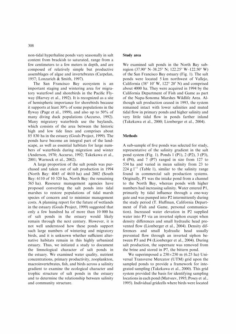
We examined salt ponds in the North Bay sub-region (37.90� N–38.25� N; 122.25� W–122.50� W)of the San Francisco Bay estuary (Fig. 1). The saltponds were located 5 km northwest of Vallejo,California (38� 10¢ W, 122� 20¢ N) and comprisedabout 4000 ha. They were acquired in 1994 by theCalifornia Department of Fish and Game as partof the Napa-Sonoma Marshes Wildlife Area. Al-though salt production ceased in 1993, the systemremained intact with lower salinities and mutedtidal flow in primary ponds and higher salinity andvery little tidal flow in ponds farther inland(Takekawa et al., 2000; Lionberger et al., 2004).

Methods

A sub-sample of five ponds was selected for study,representative of the salinity gradient in the saltpond system (Fig. 1). Ponds 1 (P1), 2 (P2), 3 (P3),4 (P4), and 7 (P7) ranged in size from 127 to534 ha and varied in mean salinity from 23 to224 g l)1 (Table 1), similar to the salinity rangefound in commercial salt production systems.Originally, P1 was the intake pond from a channelto the North Bay, whereas ponds with highernumbers had increasing salinity. Water entered P1,primarily by tidal influence through a one-waygate and was pumped into P2 intermittently duringthe study period (T. Huffman, California Depart-ment of Fish and Game, personal communica-tion). Increased water elevation in P2 suppliedwater into P3 via an inverted siphon except whendensity differences and small hydraulic head pre-vented flow (Lionberger et al., 2004). Density dif-ferences and small hydraulic head usuallyprevented flow through an inverted siphon be-tween P3 and P4 (Lionberger et al., 2004). Duringsalt production, the supernate was removed fromthe brine and stored in P7, the bittern pond.

We superimposed a 250�250 m (6.25 ha) Uni-versal Transverse Mercator (UTM) grid upon thesampled ponds to provide a framework for inte-grated sampling (Takekawa et al., 2000). This gridsystem provided the basis for identifying samplinglocations in each pond (Matveev, 1995; Posey et al.,1995). Individual gridcells where birds were located

308

in monthly surveys were identified and selected assampling locations in each pond to facilitate thestudy of trophic level relationships. Beginning inMarch 1999, 10 gridcells in which birds were ob-served during monthly surveys were randomly se-lected from each pond for nutrient, primaryproductivity, invertebrate and fish sampling. If

<10 gridcells were used by birds within a pond,additional gridcells were selected randomly.

Water quality

From February 1999 until November 2001, waterquality parameters were measured monthly in P1,

Figure 1. Former salt evaporation ponds in the Napa-Sonoma Wildlife Area located 5 km northwest of Vallejo, California, USA on

the northern edge of San Pablo Bay in the San Francisco Bay estuary.

Table 1. Average water quality values ± SD in milligrams per liter for Napa-Sonoma Ponds 1, 2, 3, 4 and 7 during 1999, 2000 and

2001

Pond Salinity (PPT) D.O. mg l)1 pH Turbidity (NTU) Temp. (�C)

1 23.1±9.4 8.7±1.5 8.1±0.3 253.9±227.0 18.2±4.8

2 23.1±8.2 8.5±1.5 8.6±0.3 82.0±44.1 16.8±4.3

3 47.6±16.1 8.3±2.2 8.4±0.2 198.4±94.8 18.0±4.7

4 169.7±70.6 6.0±4.6 7.7±0.5 96.8±97.1 19.6±5.8

7 224.3±66.4 3.6±1.8 5.9±0.8 163.4±74.4 20.5±5.4

309

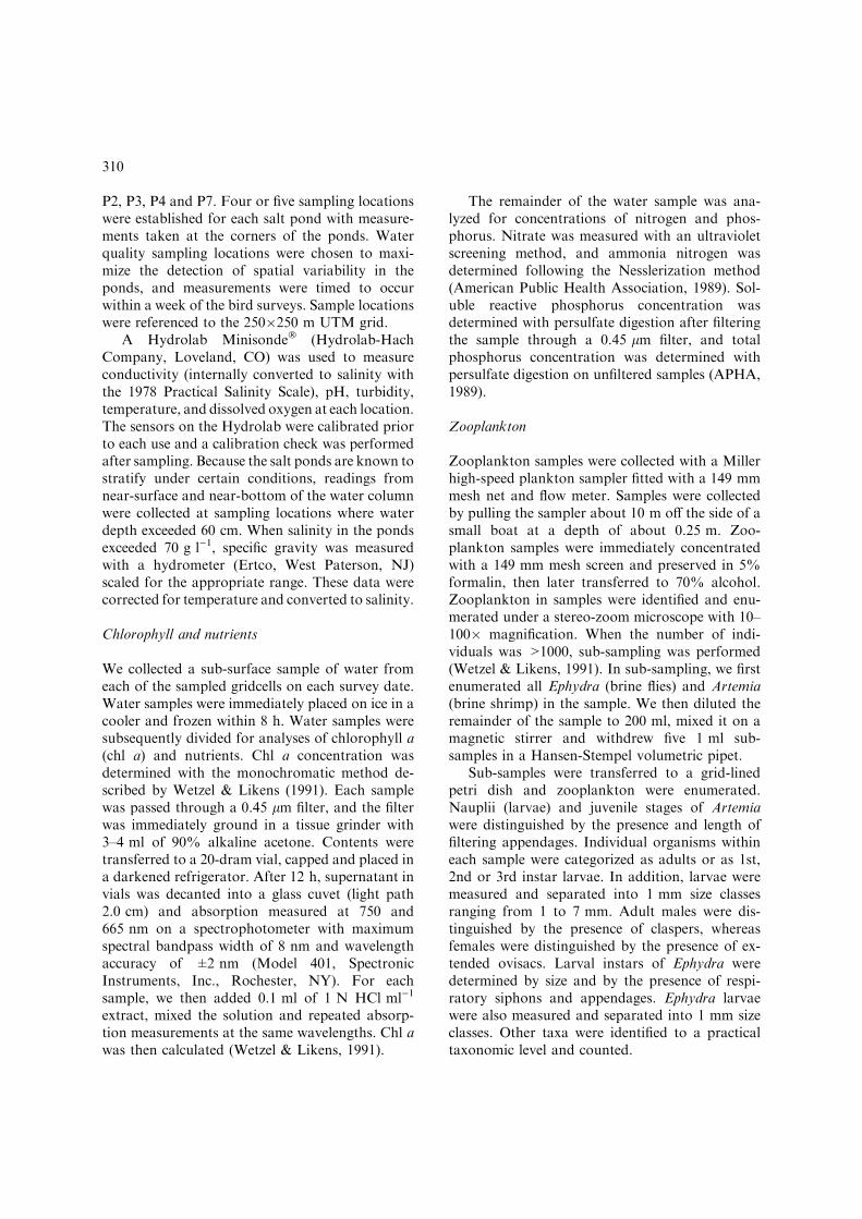
P2, P3, P4 and P7. Four or five sampling locationswere established for each salt pond with measure-ments taken at the corners of the ponds. Waterquality sampling locations were chosen to maxi-mize the detection of spatial variability in theponds, and measurements were timed to occurwithin a week of the bird surveys. Sample locationswere referenced to the 250�250 m UTM grid.

A Hydrolab Minisonde� (Hydrolab-HachCompany, Loveland, CO) was used to measureconductivity (internally converted to salinity withthe 1978 Practical Salinity Scale), pH, turbidity,temperature, and dissolved oxygen at each location.The sensors on the Hydrolab were calibrated priorto each use and a calibration check was performedafter sampling. Because the salt ponds are known tostratify under certain conditions, readings fromnear-surface and near-bottom of the water columnwere collected at sampling locations where waterdepth exceeded 60 cm. When salinity in the pondsexceeded 70 g l)1, specific gravity was measuredwith a hydrometer (Ertco, West Paterson, NJ)scaled for the appropriate range. These data werecorrected for temperature and converted to salinity.

Chlorophyll and nutrients

We collected a sub-surface sample of water fromeach of the sampled gridcells on each survey date.Water samples were immediately placed on ice in acooler and frozen within 8 h. Water samples weresubsequently divided for analyses of chlorophyll a(chl a) and nutrients. Chl a concentration wasdetermined with the monochromatic method de-scribed by Wetzel & Likens (1991). Each samplewas passed through a 0.45 lm filter, and the filterwas immediately ground in a tissue grinder with3–4 ml of 90% alkaline acetone. Contents weretransferred to a 20-dram vial, capped and placed ina darkened refrigerator. After 12 h, supernatant invials was decanted into a glass cuvet (light path2.0 cm) and absorption measured at 750 and665 nm on a spectrophotometer with maximumspectral bandpass width of 8 nm and wavelengthaccuracy of ±2 nm (Model 401, SpectronicInstruments, Inc., Rochester, NY). For eachsample, we then added 0.1 ml of 1 N HCl ml)1

extract, mixed the solution and repeated absorp-tion measurements at the same wavelengths. Chl awas then calculated (Wetzel & Likens, 1991).

The remainder of the water sample was ana-lyzed for concentrations of nitrogen and phos-phorus. Nitrate was measured with an ultravioletscreening method, and ammonia nitrogen wasdetermined following the Nesslerization method(American Public Health Association, 1989). Sol-uble reactive phosphorus concentration wasdetermined with persulfate digestion after filteringthe sample through a 0.45 lm filter, and totalphosphorus concentration was determined withpersulfate digestion on unfiltered samples (APHA,1989).

Zooplankton

Zooplankton samples were collected with a Millerhigh-speed plankton sampler fitted with a 149 mmmesh net and flow meter. Samples were collectedby pulling the sampler about 10 m off the side of asmall boat at a depth of about 0.25 m. Zoo-plankton samples were immediately concentratedwith a 149 mm mesh screen and preserved in 5%formalin, then later transferred to 70% alcohol.Zooplankton in samples were identified and enu-merated under a stereo-zoom microscope with 10–100� magnification. When the number of indi-viduals was >1000, sub-sampling was performed(Wetzel & Likens, 1991). In sub-sampling, we firstenumerated all Ephydra (brine flies) and Artemia(brine shrimp) in the sample. We then diluted theremainder of the sample to 200 ml, mixed it on amagnetic stirrer and withdrew five 1 ml sub-samples in a Hansen-Stempel volumetric pipet.

Sub-samples were transferred to a grid-linedpetri dish and zooplankton were enumerated.Nauplii (larvae) and juvenile stages of Artemiawere distinguished by the presence and length offiltering appendages. Individual organisms withineach sample were categorized as adults or as 1st,2nd or 3rd instar larvae. In addition, larvae weremeasured and separated into 1 mm size classesranging from 1 to 7 mm. Adult males were dis-tinguished by the presence of claspers, whereasfemales were distinguished by the presence of ex-tended ovisacs. Larval instars of Ephydra weredetermined by size and by the presence of respi-ratory siphons and appendages. Ephydra larvaewere also measured and separated into 1 mm sizeclasses. Other taxa were identified to a practicaltaxonomic level and counted.

310

Biomass of Artemia and Ephydra was calcu-lated from length to weight relationships andabundance. Length–weight regressions weredetermined from 60 Artemia and 32 Ephydra. Werecorded lengths (nearest 0.01 mm) under the ste-reomicroscope fitted with an ocular micrometerand preserved weight of individuals (nearest1.0 lg) on a Mettler model M1 microbalance(Mettler-Toledo, Inc., Columbus, OH). We deter-mined fresh weight from preserved weight with aconversion of 0.8, and dry weight from freshweight with a conversion of 1.1 (Wetzel, 1983).

Macroinvertebrate surveys

Benthic macroinvertebrates were sampled in P1,P2, P3 and P4. P7 was sampled on three occasions,but sampling was discontinued because inverte-brates were rare or not found at such high salini-ties. Monthly waterbird surveys were used torandomly select 10 gridcells identified by GPSlocation to sample for benthic macroinvertebrateswithin each pond. P1–P4 were sampled every othermonth beginning April 1999 to November 2000,and then in February, June and November 2001(sample frequency changed with very low waterlevels in some ponds in summer or duringinclement weather conditions in winter).

Within each gridcell, we located the center witha GPS unit, allowed the boat to drift, and thencollected three cores (about 3 m apart) with astandard Ekman grab sampler (15.2 cm3). Astandard (USA ASTME-11 Number 18) 1.0 mmmesh sieve was used to reduce cores to inverte-brates and debris that were preserved in 70%ethanol and Rose Bengal dye. The qualitativeprocedure for estimating the texture of the sub-strate was developed by a single observer, whotrained others in this characterization. Substratewas characterized as soft, medium, or hard inpenetrability, and as primarily clay, sandy, or siltyin appearance. We noted outstanding features,such as abundant shell fragments, large organicdebris, or encrusted crystalline salt.

Field samples were processed using binocularmicroscopes (3–10� power) by sorting individualinvertebrates from debris and residual sediment.Invertebrates were identified and enumerated togenus or species (when common) or family (whenuncommon) with appropriate keys (e.g., Smith &

Carlton, 1975; Morris et al., 1980). As a qualitycontrol measure, a second observer verified theidentification of 5–10% of these samples. Blottedwet weight biomass of organisms was determinedwith an Ohaus, Model 3130 scale (Pine Brook,NJ). Samples were dried in a Precision convectionoven (Winchester, VA) at 15.5 �C for 24 h todetermine dry weight.

Fish surveys

Fish species assemblages were surveyed bimonthlyfrom July 1999 until December 2000 in P1–P3(sampling in P4, which ranged to salinity 100, wasdiscontinued after no fish were detected in initialsamples; P7, with salinity >250, was presumed notto support fish life). We used bag seines to sampleshallow areas near shore and gill nets to sampledeeper areas offshore to assess the distribution andrelative abundance of both juvenile and adultfishes. Fishing effort for each gear type was stan-dardized and replicated to allow for statisticalcomparisons of fish catch among dates and sites. A5.5 m bag seine with 6.4 mm mesh in the bag and12.7 mm mesh in the wings was used alongshorelines in water <1.5 m deep. Six sites weresampled with five hauls of a bag seine at each siteby manually dragging the seine about 8 m per-pendicular or parallel to shore.

In addition, six 38.1 m long (1.8 m deep)variable-mesh monofilament gill nets with 12.7,15.4, 38.1, 50.8 and 63.5 mm square mesh panelswere fished for a maximum of 6 h, checking themevery 1–2 h to release protected fish species such asSacramento splittail (Hypomesus transpacificus)and delta smelt (Pogonichthys macrolepidothus).Individuals were identified to species in the fieldwith taxonomic keys (Miller & Lea, 1972; Moyle,1976; Eschmeyer et al., 1983; McGinnis, 1984).Fish that were not reliably identified in the fieldwere preserved and later identified by taxonomicspecialists. The first 25 individuals of each specieswere measured for standard length (to the nearestmm) and weighed (blotted wet weight biomass tothe nearest 0.1 g).

Bird surveys

We conducted monthly complete counts of the fiveponds from January 1999 to June 2001, and then

311

bimonthly counts thereafter through November2001. Observers conducted counts of species withbinoculars and spotting scopes from vantagepoints at the edge of ponds during the first week ofeach month, and locations of waterbirds wereplaced within the gridcells of each pond. Surveyswere conducted during the day within 3 h of thehighest high tide when the largest number ofwaterbirds was roosting in the salt ponds.

Identified waterbirds were separated into guildsto examine differences among foraging groups ra-ther than differences among species. These foragingguilds included: (1) sweepers – obtained prey fromthe surface, e.g., Recurvirostra americana (Ameri-can avocet); (2) shallow probers – foraged in thetop layer (<3 cm) of sediments, e.g.,Calidris mauri(western sandpiper); (3) deep probers – reacheddeeper into the substratum than shallow probers,e.g., Limosa fedoa (marbled godwit); (4) dabblers –fed in the upper water column, e.g., Anas acuta(northern pintail); (5) diving benthivores – fed indeeper water on benthic invertebrates, e.g., Aythyaaffinis (lesser scaup); (6) piscivores – fish consum-ers, e.g., Pelecanus erythrorhynchos (Americanwhite pelican); and (7) other – omnivores andincidental species including gulls.

Statistical analyses

We examined differences in salt ponds during thewinter (Dec–Feb), spring (Mar–May), summer(June–Aug), and fall (Sep–Nov) seasons, 1999–2001. Months were assigned to seasons to encom-pass the major bird migration chronology in springand fall. We computed means from repeatedmonthly water quality measurements but did notmake statistical comparisons, because samplinglocations were fixed and non-random. We com-puted means from repeated monthly or bimonthlynutrient measurements for each pond and exam-ined between-pond differences with univariateanalysis of variance (ANOVA) or multivariate(MANOVA) tests (SAS Institute, 1990). We testedfor equal variances using Levene’s test and thenused the multiple variance mixed procedure (SASInstitute, 1990) if data violated the equal varianceassumption. Because sample sizes often differedamong ponds, significant ANOVA results wereinvestigated with the Tukey–Kramer procedure

(SAS Institute, 1990) to make multiple compari-sons among pairs of means (Sokal & Rohlf, 1995).

Sampling effort for chl a, zooplankton, inver-tebrates, and fish was standardized and replicatedto allow for statistical comparisons among ponds.The results of fish sampling methods were not di-rectly comparable because species composition,numbers, and biomass differed strongly betweengear types. However, samples were standardizedfor sample size and then combined for biomassand species diversity comparisons. To ensure equalrepresentation of sampling methods in compari-sons of fish species composition between ponds,catch data were converted to proportions of thetotal catch for each gear type and then combined.Complete counts of birds were standardized byconversion to density (birds ha)1) because saltponds varied in size. We used the Shannon–Weinerindex (Krebs, 1999) to assess species diversity forbirds, fish, and invertebrates for each independentsampling event. For invertebrates, we used aMANOVA model to compare diversity indicesover time by pond (model effect) with least squaresand mean response design. ANOVA was then usedto compare individual differences among ponds ortime.

We elaborated on the between-pond compari-sons by directly examining the relationship be-tween salinity and other parameters. Weindependently examined chl a concentrations andzooplankton biomass in addition to invertebrate,fish, and bird concentrations and diversity byapplying a best-fit quadratic function to the rela-tionship with salinity. Non-metric Multidimen-sional Scaling (NMDS), a distance-basedordination method that displays multi-dimen-sional data by maximizing rank–order correlation,was used to present similarity matrix distances anddistance in ordination space on two-dimensionalplots (Clarke & Warwick, 2001). We used thePRIMER program (Plymouth Routines in Multi-variate Ecological Research, Plymouth, England)to perform NMDS on transformed data based ona Bray–Curtis similarity matrix (Bray & Curtis,1957), and visually compare species compositionamong samples in two dimensions. We averagedsample values by season to simplify the displayand associated larger diameter circles withincreased salinity to accentuate the relationship

312

between salinity and species composition (Clarke& Warwick, 2001). We used analysis of similarities(ANOSIM, PRIMER) to further investigatecommunity differences among ponds with 5000permutations to compare overall and pair-wiseeffects of pond differences on species composition.PRIMER provides Global R and pairwise R sta-tistics that provide a measure of the differencebetween rank dissimilarities within and amonggroups (Sommerfield et al., 2002). Stress valuesrepresent how well the multi-dimensional rela-tionship between variables is represented in thetwo-dimensional plot; although stress parameterschange according to quantity of data as well as thenumber of dimensions, Clarke & Warwick (2001)suggest that stress <0.05 is excellent but stress<0.10 is a good ordination, whereas stress >0.3suggests that the ordination plot is not interpret-able. For all analyses, results were deemed signif-icant when p £ 0.05.

Results

Water quality

Salinity varied widely throughout the study,ranging from 23.1 to 224.3 g l)1 (Table 1, Fig. 2).The intake pond (P1) and an interior pond (P4)showed the greatest temporal variation in salinity.Ponds varied more seasonally than they didannually, especially in the higher salinity ponds(Fig. 2). Salinity was lowest following late winterrainfall and increased to peak concentrations inthe late summer. The pH of the system was alka-line, but the water in P7, a bittern pond that wasoften very shallow with few areas to sample, wasacidic throughout the year (Table 1). Turbiditywas generally high in P3, coincident with seasonalwinds. Water temperature ranged from 9 to 30 �C,with greatest extremes in P1 and P4, ponds thatalso had the greatest changes in water levels. De-creased water levels combined with elevated tem-peratures resulted in low dissolved oxygenreadings in P4 during the summer months.

Nutrients

Nutrient concentrations varied among ponds andseasons (Table 2). Nitrate (NO3–N) concentration

ranged from 0.306 to 8.05 mg l)1 (Fig. 3). Nitratewas greater in P4 than in P1 and P2 (F3,25=3.89,p<0.021). Ammonia (NH3–N) concentrationsranged from 0.409 to 18.2 mg l)1 (Fig. 3).Ammonia was greater in P4 than in P1–P3 (F3,24=25.23, p<0.0001). Average soluble reactive phos-phorus (SRP) concentration ranged from 0.151 to3.21 mg l)1 (Fig. 3). Overall, SRP concentrationwas lower in P4 than in P2 or P3 (F3,25=3.33,p=0.036). Average total phosphorus (TP) con-centration ranged from 0.29 to 4.88 mg l)1

(Fig. 3). TP concentration was greater in P2 and P3than in P4 (F3,25=4.72, p=0.0096). Nitrogen tophosphorus (N:P) ratios ranged from 0.3 to 3.2 inP1, from 0.7 to 3.4 in P2, from 0.9 to 7.5 in P3 andfrom 2.3 to 30.3 in P4. N:P ratios in P4 were >10.0on 4 of 7 dates, but <10.0 in the other ponds on alldates.

Primary productivity

Mean annual chl a concentration was higher in P3and P4 than in P1 (Table 3). Seasonal change inchl a concentration was most pronounced in P4,and least pronounced in P1 and P2 (Fig. 4a). Chl aconcentration was greater in P3 and P4 than in P1.However, the mean annual concentration in P4reflected exceptionally high chl a concentrations(130.0 mg m)3) measured in the winter (Fig. 4a).Overall, chl a generally increased with salinity, butonly P1 was significantly lower than the otherponds (Table 3; F3,164=4.46, p=0.0048). Patternsin phaeophyton concentrations by pond weresimilar to chl a (F3,164=4.46, p=0.0049) and werehigher in P2, P3, and P4 than in P1 (Table 3).

Among all ponds, chl a concentration wasnegatively correlated with total zooplankton bio-mass (intercept=1.2266, slope=)0.4547, adjustedr2=0.17, p<0.0001). Similarly, chl a concentrationin P4 was negatively correlated with Artemia bio-mass (intercept=12.333, slope=)0.7689, adjustedr2=0.331, p<0.0001).

Zooplankton

Twenty zooplankton taxa were identified in thesalt ponds. Eight taxa were recorded in lowersalinity ponds (P1 and P2), seven were recordedin P3 and only five taxa were recorded in P4 andP7. Seasonally, more taxa were recorded during

313

0

100

200

300

400

500

600

700

800

900

Jan-99 Jul-99 Feb-00 Aug-00 Mar-01 Sep-01

Tu

rbid

ity

(NT

U)

Dis

solv

ed O

xyge

n(m

g•l-1

)

Sep-01Mar-01Aug-00Feb-00Jul-99Jan-99

18

16

14

12

10

8

6

4

2

0

3

4

5

6

7

8

9

10

Jan-99 Jul-99 Feb-00 Aug-00 Mar-01 Sep-01

pH (S

. U.)

Salin

ity (

g•l-1

)

Sep-01Mar-01Aug-00Feb-00Jul-99Jan-99

300

250

200

150

100

50

0

0

5

10

15

20

25

30

35

Jan-99 Jul-99 Feb-00 Aug-00 Mar-01 Sep-01

Tem

per

atu

re (

ºC)

Pond 7

Pond 4

Pond 3

Pond 2

Pond 1

(a)

(c)

(e)

(d)

(b)

Figure 2. Salinity (g l)1), dissolved oxygen (mg l)1), pH (SU), turbidity (NTU), temperature (�C) for Ponds 1, 2, 3, 4 and 7 in the

Napa-Sonoma Marshes from 4 to 5 sampling locations per pond, Feb 1999–Nov 2001.

Table 2. Average dissolved nutrient concentrations ± SD (lg l)1) for Napa-Sonoma Ponds 1–4 during 1999 and 2000. Means that are

not significantly different (Tukey–Kramer) are indicated by similar superscripts

Pond NO3 mg l)1 NH3–N mg l)1 SRP mg l)1 TP mg l)1

1 1.57a±1.1 5.56a±2.8 2.18ab±0.8 2.17ab±0.8

2 1.47a±1.7 6.24a±1.1 3.21b±1.3 3.34b±1.4

3 3.30ab±2.6 7.21a±3.0 2.57b±0.9 2.71b±1.2

4 4.02b±1.3 15.42b±2.2 1.25a±1.7 1.16a±1.2

314

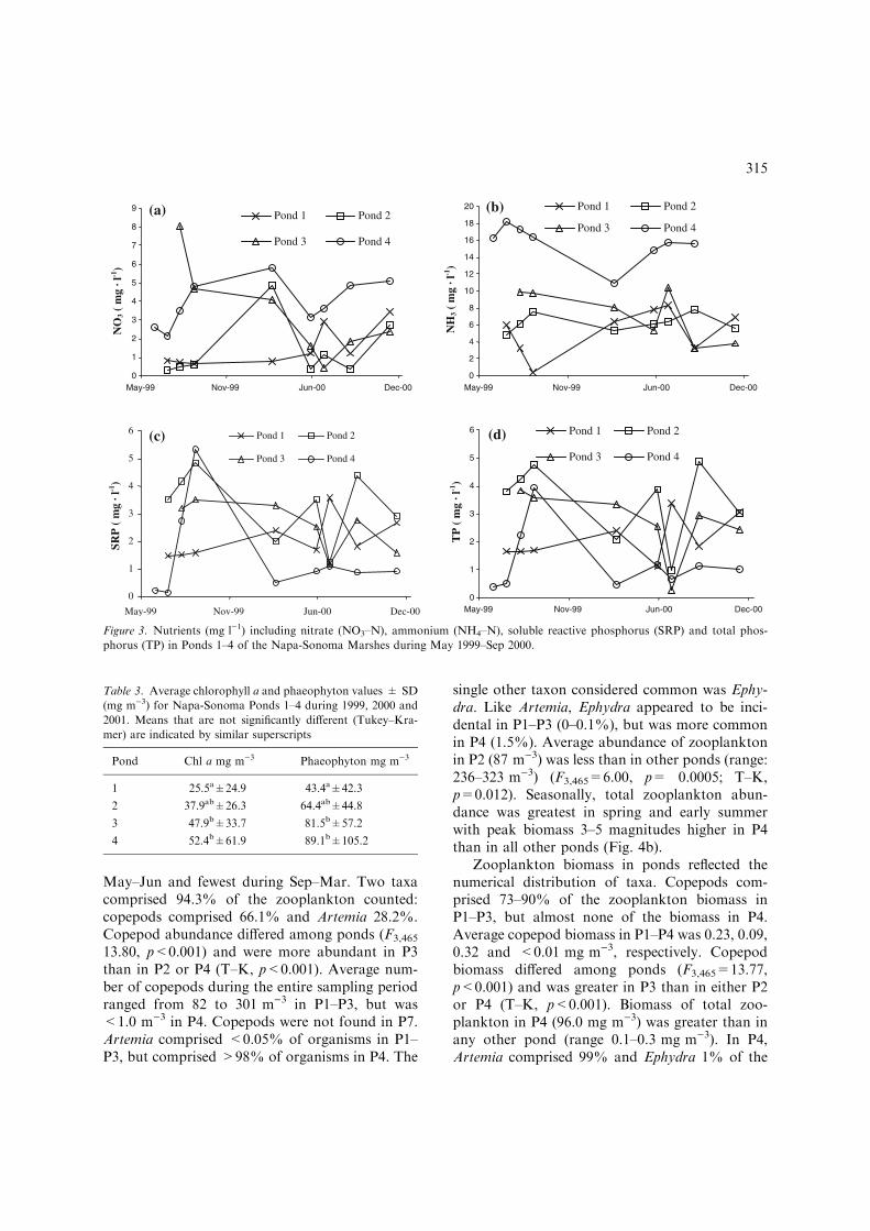
May–Jun and fewest during Sep–Mar. Two taxacomprised 94.3% of the zooplankton counted:copepods comprised 66.1% and Artemia 28.2%.Copepod abundance differed among ponds (F3,465

13.80, p<0.001) and were more abundant in P3than in P2 or P4 (T–K, p<0.001). Average num-ber of copepods during the entire sampling periodranged from 82 to 301 m)3 in P1–P3, but was<1.0 m)3 in P4. Copepods were not found in P7.Artemia comprised <0.05% of organisms in P1–P3, but comprised >98% of organisms in P4. The

single other taxon considered common was Ephy-dra. Like Artemia, Ephydra appeared to be inci-dental in P1–P3 (0–0.1%), but was more commonin P4 (1.5%). Average abundance of zooplanktonin P2 (87 m)3) was less than in other ponds (range:236–323 m)3) (F3,465=6.00, p= 0.0005; T–K,p=0.012). Seasonally, total zooplankton abun-dance was greatest in spring and early summerwith peak biomass 3–5 magnitudes higher in P4than in all other ponds (Fig. 4b).

Zooplankton biomass in ponds reflected thenumerical distribution of taxa. Copepods com-prised 73–90% of the zooplankton biomass inP1–P3, but almost none of the biomass in P4.Average copepod biomass in P1–P4 was 0.23, 0.09,0.32 and <0.01 mg m)3, respectively. Copepodbiomass differed among ponds (F3,465=13.77,p<0.001) and was greater in P3 than in either P2or P4 (T–K, p<0.001). Biomass of total zoo-plankton in P4 (96.0 mg m)3) was greater than inany other pond (range 0.1–0.3 mg m)3). In P4,Artemia comprised 99% and Ephydra 1% of the

Pond 4Pond 3

Pond 2Pond 1

NO

3 ( m

g · l

-1)

Dec-00Jun-00Nov-99

7

8

9

3

4

5

6

0May-99

1

2

NH

3 ( m

g · l

-1)

Pond 4Pond 3

Pond 2Pond 1

Dec-00Jun-00Nov-99May-99

20

18

16

14

12

10

8

6

4

2

0

SRP

( m

g · l

-1)

Pond 4Pond 3

Pond 2Pond 1

Dec-00Jun-00Nov-99

6

5

4

3

2

1

0

May-99

TP

( m

g· l

-1)

Pond 4Pond 3

Pond 2Pond 1

Dec-00Jun-00Nov-99May-99

6

5

4

3

2

1

0

(a)

(c) (d)

(b)

Figure 3. Nutrients (mg l)1) including nitrate (NO3–N), ammonium (NH4–N), soluble reactive phosphorus (SRP) and total phos-

phorus (TP) in Ponds 1–4 of the Napa-Sonoma Marshes during May 1999–Sep 2000.

Table 3. Average chlorophyll a and phaeophyton values ± SD

(mg m)3) for Napa-Sonoma Ponds 1–4 during 1999, 2000 and

2001. Means that are not significantly different (Tukey–Kra-

mer) are indicated by similar superscripts

Pond Chl a mg m)3 Phaeophyton mg m)3

1 25.5a±24.9 43.4a±42.3

2 37.9ab±26.3 64.4ab±44.8

3 47.9b±33.7 81.5b±57.2

4 52.4b±61.9 89.1b±105.2

315

biomass. Seasonally, total zooplankton biomasswas greatest in spring and summer, except in P2where it was low on most dates.

Macroinvertebrates

Species diversity (Shannon–Wiener) of benthicmacroinvertebrates among ponds and time periodssampled (approximately bimonthly) differed sig-nificantly (MANOVA, F36,299=23.90, Wilk’sk=0.02, p<0.0001). Mean overall diversity dif-fered significantly among ponds (F3,48=17.80,p<0.001). P1 and P2 were different from P3 andP4 (T–K p=0.0002; Table 4). Diversity was gen-erally higher and similar in P1 and P2 relative toP3 and P4. One-way ANOVA and Tukey–Kramertests indicated that diversity in P1 and P2 did not

differ significantly in 1999 and early 2000 (F3,116=10.99–205.51, p<0.0001) but were significantlyhigher in P1 than P2 in May 2000 (F3,116=34.30,p<0.0001) and higher in P2 after May 2000

0

20

40

60

80

100

120

140

Feb-00 Mar-00 May-00 Jun-00 Aug-00 Oct-00 Nov-00 Jan-01

Chl

a m

g ·

m -3

Pond 1

Pond 2

Pond 3

Pond 4

0

0.2

0.4

0.6

0.8

1

1.2

1.4

1.6

1.8

2

Feb-99 May-99 Aug-99 Nov-99 Mar-00 Jun-00 Sep-00 Jan-01

Bio

mas

s m

g ·

m -3

Pon

ds 1

-3

0

50

100

150

200

250

300

350

400

450

500

Biom

ass mg · m

-3 Pond 4

Pond 1

Pond 2

Pond 3

Pond 4

(a)

(b)

Figure 4. (a) Chlorophyll a (mg m)3) and (b) zooplankton (mg m)3) in Ponds 1–4 of the Napa-Sonoma Marshes, May 1999–Sep 2000.

Table 4. Mean Shannon–Wiener diversity indices ± SD from

1999 to 2001. Fish were not detected in Napa-Sonoma Ponds 4

and 7. Invertebrates were collected too infrequently in Pond 7

for comparison. Means that are not significantly different

(Tukey–Kramer) are indicated by similar superscripts

Pond Mean bird H¢ Mean fish H¢ Mean invert H¢

1 1.75c±0.5 1.31b±0.5 0.96b±0.3

2 1.40b±0.7 0.53a±0.3 1.12b±0.3

3 1.58bc±0.4 0.84a±0.2 0.54a±0.3

4 1.83c±0.8 – 0.51a±0.2

7 0.60a±0.9 – –

316

(F3,116=57.11–139.05, p<0.0001). Mean separa-tion tests indicated that diversity in P3 and P4 wassimilar on 6 of 10 intervals sampled in 1999 and2000, but like P1 and P2, differed significantly in2001. Diversity in P1 and P4 were similar (Jul1999, Jan and Mar 2000) until 2001 when all pondswere dissimilar during all sampling intervals.

Diversity in P1 and P2 was represented by50–55 taxa, many of which were uncommon, andhigh densities of individuals from just 3–4 taxa. P3(25 taxa) and P4 (12 taxa) usually had lowernumbers of taxa and similarly high densities in 2–4taxa. Heteromastus sp. (polychaete), Gemma sp.(bivalve), Corophium sp. and Ericthonius sp.(amphipods) dominated taxa in P1 and P2, Poly-dora sp., Capitella sp. (polychaetes), Corophiumsp., and occasionally Streblospio sp. (polychaete)and Corixidae (waterboatman insect) dominatedP3, and Artemia and Ephydra dominated P4.

Fish

From July 1999 to December 2000, a total of 4334fish representing 16 species was captured from P1to P3. Gill netting yielded 730 fish (16.8%),whereas bag seining yielded 3604 fish (83.2%).Fish abundance from gill nets was high in both P1(343 fish) and P2 (368 fish), with far fewer fishcaptured in P3 (19 fish). No fish were captured inP4. By comparison, bag seines indicated that fishabundance was highest in P1 (2694 fish), followedby P3 (779 fish), and P2 (131 fish). Combinedbiomass was greatest in P1 and P2, and muchlower in P3.

Gill netting and bag seining sampled differentsegments of the fish species assemblage in eachpond. In P1, American shad (Alosa sapidissima,37.3%), striped bass (Morone saxatilis, 42.9%),and striped mullet (Mugil cephalus, 8.5%) werecaptured in gill nets, whereas Pacific staghornsculpin (Leptocottus armatus, 51.4%) and yellow-fin goby (Acanthogobius flavimanus, 41.6%) werecaptured in bag seines. In P2, gill net catchesconsisted almost exclusively of striped bass(94.3%), while bag seine catches consisted mostlyof inland silverside (Menidia beryllina, 42.0%) andstriped bass (32.8%). In P3, striped bass (47.4%),longjaw mudsucker (Gillichthys mirabilis, 36.8%),and yellowfin goby (15.8%) were caught in gillnets, and longjaw mudsucker (45.3%), Shimofuri

goby (Tridentiger bifasciatus, 28.6%), and inlandsilverside (20.9%) were captured in bag seines.Shannon–Wiener diversity differed significantlyamong ponds (F2, 22=10.40, p=0.0007). P1 hadthe highest overall diversity, significantly higherthan P2 and P3 (p=0.0005), which did not differ(p=0.318; Table 4).

Birds

Mean diversity differed significantly among ponds(F4,146=4.84, P=0.0011). P7 had the lowestdiversity and differed significantly from all otherponds. Sixty-five species were recorded in allponds, comprising several foraging guilds (seeTakekawa et al., 2001). Diving benthivores com-prised the majority of birds in all ponds followedby shallow probers. Surface feeders, dabblers,piscivores, and deep probers made up theremainder. P4 contained the greatest density ofbirds, whereas P1–P3 and P7 contained substan-tially less.

P1–P4 supported the majority of diving ben-thivores, primarily diving duck species. P2 sup-ported almost exclusively diving ducks,representing over 95% of the birds counted in thepond. In P3, diving ducks comprised 70% of thebirds counted in the pond. P7 had very few birdspresent year-round. Density of non-piscivorousbirds was highest in Pond 1, and lowest in Pond 3.Piscivorous birds were much higher in Pond 1compared with other ponds.

Waterbirds were most diverse and abundant onP1 (48 species and 23% of the total birds) and P4(46 species and 46% of the total birds), butdiversity on these ponds did not differ significantlyfrom P3 (T–KP3,P4, p=0.1293; Table 4). In sum-mer, P4 contained few diving benthivores relativeto shorebirds, particularly shallow probers.

Trophic variation and the salinity gradient

The relationship between salinity and chl a(Fig. 5a) fit a quadratic equation with lowestconcentrations at mid salinity (r2=0.4201,p=0.0499). Conversely, the relationship betweensalinity and zooplankton (Fig. 5b) was inverse,with highest concentrations of zooplankton atmid-salinities (r2=0.3661, p=0.0002). A test of therelationship between invertebrate biomass and

317

salinity (Fig. 5c) showed that salinity explained16.8% of the variation in biomass (p=0.0176) and27.8% of the variation in invertebrate diversity(p=0.0008). Macroinvertebrate biomass anddiversity fit a quadratic curve similar to chl a(Fig. 5c), but with much higher levels at lowsalinities. Biomass of fishes decreased with salinity(r2=0.5667, p=0.0002; Fig. 5d), but the relation-ship between salinity and diversity was not sig-nificant (r2=0.0895, p=0.3913). Finally, birddensity and diversity fit quadratic equations withhighest levels at mid-salinities (Fig. 5e); densitywas not well explained by salinity (r2=0.0501,p=0.0312), whereas and bird diversity (Fig. 5e) fita quadratic equation with highest levels at mid-salinities (r2=0.2308, p<0.0001).

Trophic similarity by season and salinity

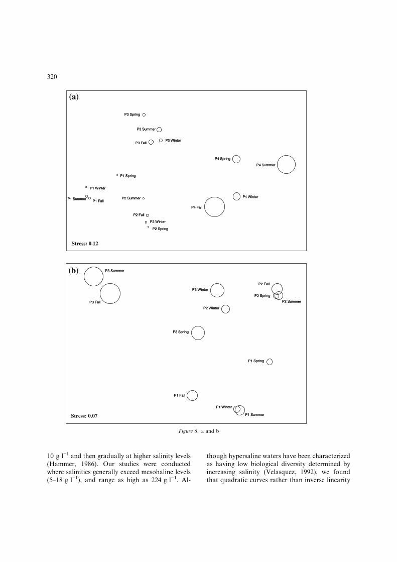
The NMDS ordination showed that macroinver-tebrate community composition was consistentwithin ponds across seasons and varied withsalinity (Fig. 6a). Each pond had a cluster inFigure 6a, indicating that macroinvertebratecommunity composition was consistent withinponds for all seasons. Composition also variedwith salinity, as indicated by left to right increasein salinity (bubble size) in Figure 6a. The macro-invertebrate ordination had a fairly good rela-tionship with a low stress value of 0.12. P1 and P2had comparable composition of taxa, but abun-dances of these common taxa differed over time.P3 had a distinct invertebrate community thatdiffered from P1, P2 and P4, and the community ofP4 vastly differed from P1, P2 and P3, reflectingthe much higher salinity in P4 (Table 1).

Seasonal differences in invertebrate communi-ties were not consistent, but spring was most oftenrepresented on the perimeter of pond groupings inordination space (Fig. 6a). ANOSIM determinedthat the composition of invertebrate communitiesdiffered significantly among ponds (GlobalR=0.779, p<0.0001; Clarke & Warwick, 2001). Inpairwise tests of the ponds, P1 and P2 communitycomposition differed significantly but at a lowerlevel of significance (p=0.001) than all other pondpairs (p<0.0001).

Fish community composition differed signifi-cantly among ponds overall (Global R=0.313,p<0.0001) and across pairwise comparisons

(p<0.0001). The excellent fit for the NMDSrelating fish communities across ponds(stress=0.07) suggests that seasonal variation inspecies composition may be closely related tosalinity. Samples with similar salinity values haddissimilar species composition, whereas sampleswith dissimilar salinities had similar species com-position, but within-pond samples were mostsimilar across seasons (Fig. 6b). During summerand fall, the fish ordination plot suggested that P3had the most dissimilar fish species compositionfrom other ponds, and its community compositionwas closer to P3 in winter and spring than to anyother pond (Fig. 6b).

Although species composition within pondswas less clearly delineated for birds than other taxa(except P7), community composition differed sig-nificantly among ponds overall (Global R=0.398,p<0.0001) and across pair-wise comparisons(p<0.0001). The NMDS analysis (stress=0.13)suggested a strong influence of salinity on avianspecies composition in P7 and in P4 (Fig. 6c), butP4 values were more similar to P1–P3. P7 in thespring was most dissimilar to all other pond andseason combinations.

Discussion

The wetland classification system for the UnitedStates (Cowardin et al., 1979) recognizes estuarinewetlands modified by salinity, but poorly distin-guishes the hyperhaline (haline is used to indicatean ocean salt source, but salinity is used inter-changeably here unless referring to a specificwetland type) communities that we studied inthe San Francisco Bay salt ponds. For example,P1 and P2 had very similar salinity, dissolvedoxygen, and pH patterns, but they would beseparated into mixohaline (0.5–30 g l)1) and euh-aline (30–40 g l)1) classes. P3, P4 and P7 would beclassified under the single modifier of hyperhaline(>40 g l)1), despite great differences in their eco-logical communities. Inland saline classificationsystems also were inappropriate for classifying theecological communities we studied. Javor (1989)used microorganisms to describe four hyperhalineclasses characterized by macroalgae and fish(60–100 g l)1), halophilic species (100–140 g l)1),Dunaliella and Artemia (140–300 g l)1), and low

318

productivity Dunaliella and bacteria (300–360 g l)1), but higher trophic levels were notconsidered in his definitions. Thus, we used mix-ohaline (0.5–30 g l)1), and low (31–80 g l)1), mid(81–150 g l)1), and high (>150 g l)1) hyperhaline

classes to better represent the distinctive trophiccommunities we observed.

Most studies of hypersaline systems have beenconducted in interior salt lakes where speciesrichness decreases steeply from freshwater to

Zoo

plan

kton

(m

g · m

-3)

300200100

Salinity (g · l-1)

0

500

400

300

200

100

0

R2 = 0.3661

Chl

a (

mg

· m-3

)

Salinity (g · l-1)

3002001000

70

60

50

40

30

20

10

0

R2 = 0.4201

R2 = 0.1678

R2 = 0.2781

0

1

2

3

4

5

6

7

8

9

0 100 200 300Salinity (g · l -1)

0

0.2

0.4

0.6

0.8

1

1.2

1.4

1.6

1.8

Diversity H

'

Mac

roin

vert

ebra

te b

iom

ass

(m

ean

g · s

ampl

e-1

)

R2 = 0.5667

R2 = 0.0895

0

2000

4000

6000

8000

10000

12000

14000

16000

18000

0 20 40 60

Salinity (g · l -1)

0

0.5

1

1.5

2

2.5

Diversity H

'

Fis

h bi

omas

s (m

ean

· sam

ple-1

)

R2 = 0.0501

R2 = 0.2308

0

10

20

30

40

50

60

70

80

90

0 50 100 150 200 250 300

Salinity (g · l -1)

0

0.5

1

1.5

2

2.5

3

3.5

Diversity H

'

Bir

d de

nsit

y (c

ount

· ha

-1)

(a)

(c)

(e)

(b)

(d)

Figure 5. (a) Chlorophyll a (mg m)3); (b) zooplankton (mg m)3); (c) macroinvertebrate biomass (mg m)3) and diversity (H¢); (d) fishbiomass (mg m)3) and diversity (H¢); and (e) avian counts (birds ha)1) and diversity (H¢) across salinities in Ponds 1–4 of the Napa-

Sonoma Marshes. Biomass (circles; solid line) and Shannon–Weiner species diversity (H¢: squares; broken line) are shown for (c)

macroinvertebrates, (d) fish and (e) birds along with the best-fitting curves and regression coefficients for each. All relationships were

significant (p<0.05) except for fish species diversity (p=0.3913).

319

10 g l)1 and then gradually at higher salinity levels(Hammer, 1986). Our studies were conductedwhere salinities generally exceed mesohaline levels(5–18 g l)1), and range as high as 224 g l)1. Al-

though hypersaline waters have been characterizedas having low biological diversity determined byincreasing salinity (Velasquez, 1992), we foundthat quadratic curves rather than inverse linearity

P3 Summer

P3 Fall

P1 Fall

P3 Spring

P3 Winter

P2 Winter

P1 Spring

P1 Summer

P1 Winter

P2 Spring

Stress: 0.07

P2 Summer

P2 Fall

P3 Summer

P3 Fall

P1 Fall

P3 Spring

P3 Winter

P2 Winter

P1 Spring

P1 Summer

P1 Winter

P2 Spring

P2 Summer

P2 Fall

P4 Summer

P4 Spring

P4 Winter

P4 Fall

P1 Spring

P1 FallP1 Summer

P1 Winter

P2 Fall

P2 Spring

P2 Winter

P2 Summer

P3 FallP3 Winter

P3 Spring

P3 Summer

Stress: 0.12

P4 Summer

P4 Spring

P4 Winter

P4 Fall

P1 Spring

P1 FallP1 Summer

P1 Winter

P2 Fall

P2 Spring

P2 Winter

P2 Summer

P3 FallP3 Winter

P3 Spring

P3 Summer

(a)

(b)

Figure 6. a and b

320

best described the relationship of biomass tosalinity in salt ponds of the San Francisco Bayestuary (Fig. 5). A large proportion of the vari-ation in biomass was explained by salinity forprimary producers and primary consumers, andthis relationship changed at higher salinities.Primary productivity biomass was highest undermid and high salinity conditions, whereas zoo-plankton biomass was highest under mid-salinityconditions. Changing biomass at higher salinitieswas likely often preceded by a shift in speciescomposition. Copepods predominated in mid-salinity ponds P1–P2, but were replaced by Art-emia and Ephydra in P4. Average zooplanktonbiomass in P4 was several orders of magnitudegreater than in less saline ponds, due primarily tolarge concentrations of Artemia in this hyperh-aline system.

Our analyses showed that salinity explained lessof the variation in biomass for higher trophiclevels than for lower ones. Macroinvertebratebiomass was highest in mixohaline P1, but thebiomass of hypersaline ponds (P4, and also P3

toward the end of the study) was only slightlylower because they included large numbers ofArtemia and Ephydra. Invertebrates underwent achange in community composition that resulted inan increase in biomass of Artemia following a de-cline in biomass of copepods, but fish as a groupexhibit less variability in salinity tolerance andcannot survive >80 g l)1; thus, they cannot shiftspecies composition. Although the relationshipbetween fish biomass and salinity was strong(r2=0.5667), this was an exception to the qua-dratic relationships because no fish were foundabove the low hyperhaline ponds. The relationshipbetween bird density (as an index of biomass) andsalinity was weak (r2=0.0360), but the highestdensity of birds was found in the low to midhyperhaline ponds (Fig 5e). Bird density andsalinity followed a similar quadratic model atSouth Bay salt ponds (Warnock et al., 2002).Warnock et al. (2002) found a poorer fit forpiscivorous than for non-piscivorous birds, possi-bly reflecting the greater numbers of fish in mix-ohaline ponds.

P7 Winter

P7 Spring

P7 Fall

P7 Summer

P2 Summer

P3 Summer

P3 Fall

P1 Summer

P2 Fall

P3 Spring

P2 Winter

P2 Spring

P3 Winter

P1 Winter

P4 Winter

P4 SpringP1 Spring

P1 Fall

P4 FallP4 Summer

Stress: 0.13

P2 Summer

P3 Summer

P3 Fall

P1 Summer

P2 Fall

P3 Winter

P1 Winter

P4 Winter

P4 SpringP1 Spring

P1 Fall

P4 FallP4 Summer

(c)

Figure 6. Non-metric Dimensional Scaling (NMDS) bubble plots across salinities (increasing diameter bubble with higher salinity) and

seasons in Ponds 1–4 of the Napa-Sonoma Marshes, 1999–2001 for (a) macroinvertebrates (stress=0.12), (b) fishes (stress=0.07), and

(c) birds (stress=0.13). Low stress (excellent <0.05; good <0.010; uninterpretable >0.3; Clark & Warwick, 2001) indicates a close

representation of species composition differences in ordination space.

321

Descriptions of hypersaline systems suggestthat as a general rule, species diversity decreaseswith salinity (Hammer, 1986; Williams et al., 1990;Williams, 1998). However, we found that similarto biomass, the relationship of salinity and speciesdiversity in upper trophic levels followed quadraticcurves (Fig. 5c–e). This was probably due to shiftsin species composition, following salinity regimes,within these larger taxonomic groups. However,macroinvertebrates and fish did not respond tosalinity changes as quickly as birds because com-munity composition inside the ponds was depen-dent upon the source populations within the pondsand the opportunistic immigration of organismsinto the ponds.

Diversity in the mid hyperhaline was lowest formacroinvertebrates and highest for fishes andbirds. Similar to our findings, Britton & Johnson(1987) found highest biodiversity at mid hyperha-linity salt ponds in the Camargue estuary insouthern France, but decreasing species richnesswith increasing salinity.

Seasonal variation

Britton & Johnson (1987) found that the regularseasonal cycle of salinity in salt ponds resulted ina predictable food supply and abundant avi-fauna. We found cyclical patterns of physicaland biological variables with salinity, but theregularity of these patterns was obscured bychanges in water management during our stud-ies. Water quality (Fig. 2) generally followedannual weather patterns. The lowest salinitylevels were recorded in winter (February) andhighest in late summer (August), but salinitiesgradually increased overall during the study(Fig. 2a). Dissolved oxygen was inversely relatedto salinity and temperature and reached anoxiclevels (<2 mg ml)1) in P4 and P7.

The limited inflow to the pond system createdgreater dependence on nutrient recycling throughremineralization and N-fixation in higher salinityponds. Intake water accounted for the primary in-put of nutrients intoP1 available for transformationby microbial organisms. Allochthonous nutrientsources also increased in importance as water wasmoved through the ponds and nutrients weretransformed and depleted. Bacterial N-fixation andtransformation of phytoplankton may have influ-

enced the gradual increase in nitrate in highersalinity ponds.

Effects of salinity and evaporation were great-est on P4 with the lowest influx of water, con-tributing to the higher concentrations of bothmeasured forms of nitrogen. Ammonia graduallyincreased from P1 to P3, but doubled from P3(7.21 mg l)1) to P4 (15.42 mg l)1). This may beattributed to animal waste (i.e., zooplankton,birds) or decomposition of Artemia that exceededbacterial oxidation and phytoplankton uptake. Asimple feedback loop in the form of primary pro-ducers, grazers, higher consumers, and decom-posers may be occurring in P4. Also, phosphoruswas slightly higher in P2 than in other ponds; thispond was managed to attract waterfowl for hunt-ing and stocked with fish, which may explain theelevated phosphorus.

Seasonal maximum macroinvertebrate biomasswas recorded in mid hyperhaline P4 during springand coincided with the largest number of foragingbirds at the ponds. Salinity changes in the pondsfollowed a seasonal pattern, but changes inmacroinvertebrate diversity did not. The waterregime on P1 was muted tidal flow influencedlargely by changes in adjacent estuarine waters,and the diversity of taxa in this pond was generallysimilar to that found in the North Bay sub-region(Miles, unpublished data). Water quality anddiversity in P2 was similar to that in P1, except inSeptember 2000; water management on P2 mayhave been altered around that sampling interval.The temporal pattern of species diversity wassimilar in P3 and P4, but changes in P3 were fol-lowed by changes in P4 at subsequent samplingintervals, e.g., peaks in diversity in P3 during Jul1999, Mar 2000, and Feb 2001 were followed bypeaks in P4 during Sep 1999, May 2000 and afterJun 2001.

The largest densities of waterbirds were seen inspring, with the next largest number of birds ob-served in winter (Takekawa et al., 2001). Mostmigratory bird species were not present in theestuary during summer, and we counted fewerbirds in fall compared with spring when the largestnumber of waterbirds was counted. Althoughspecies composition did exhibit some seasonalvariability, there was a greater degree of similaritywithin ponds than within seasons, even whensalinity levels were similar (Fig. 6). Thus, factors

322

other than salinity seemingly influenced speciescomposition in ponds.

Factors other than salinity

We measured seasonal variation in biomass anddiversity among trophic levels across a salinitygradient, but we did not control for differencesamong or within ponds because we lackedreplication in this single system. Factors otherthan salinity may have greatly influenced thesystem, such as hydrologic patterns, ioniccomposition, oxygen content, biological inter-actions, and water depth that might affect com-munity structure (Carpelan, 1957; Anderson,1970; Williams et al., 1990; Velasquez, 1992;Williams, 1998).

Hydrologic patternsIn northern San Francisco Bay, salinities maybecome diluted to oligohaline levels (0.5–5 g l)1)in late winter, but average salinities in the saltponds typically remained above mesohaline levelsand were influenced by rainfall and evaporativeloss. Fauna in even the mixohaline salt pondsdiffered from euryhaline estuarine species in saltponds of southern France (Britton & Johnson,1987) and impoverished fauna at hypersalinity wasattributed to lagoon-type confinement. Similarly,Carpelan (1957) described South Bay salt ponds asmore similar to littoral lagoons than estuarinewetlands.

Ionic composition and nutrientsSpecies diversity quickly decreases in low hyperh-aline ponds when carbonates precipitate (70 g l)1),remains constant in mid hyperhaline ponds whenCaSO4 precipitates (150 g l)1), and declines inhigh hyperhaline ponds where few species ofinvertebrates survive (300 g l)1; Britton & John-son, 1987). Fish are absent above the lowhyperhaline, but Artemia and Ephydra reachmaximum density at high hyperhaline, althoughthey may survive across a much wider range ofsalinities (Maffei, 2000). Molluscan species withcarbonate shells tend to disappear above lowhypersalinity, and our collections indicated fewclams in P3 and P4. Salt ponds typically have lowN and P, restricting plant growth (Britton &Johnson, 1987) and increasing nitrate with salinity,

although our results showed nitrates were highlyvariable (Fig. 3). P1–P2 had beds of Ruppiamaritima, but hyperhaline ponds lacked any sub-mergent macrophytes.

Dissolved oxygenSherwood et al. (1992) reported an inverse rela-tionship between oxygen content and salinityranging from 8.85 mg l)1 at 5 g l)1 to 1.7 mg l)1

at 260 g l)1. Williams (1998) suggested that respi-ratory breakdown occurs at �2 mg l)1. In the midand high hyperhaline ponds, oxygen dropped be-low the respiratory threshold in summer months.The lack of oxygen in those ponds may haveinfluenced the biomass of invertebrates.

Biological interactionsOur chl a and zooplankton data illustrate foodweb interactions at several trophic levels. First, wefound a weak negative correlation of zooplanktonbiomass with chl a. The negative relationship be-tween biomass of Artemia and chl a was strongerin P4. Grazing by Artemia probably reduced algaldensities, resulting in low chl a concentrationsduring summer. In turn, increased chl a concen-trations in winter were probably influenced bydecomposition of Artemia and subsequent in-creased ammonia that benefited phytoplankton.Artemia was the key taxon in the simple food webof P4. In this fishless pond, high densities andbiomass of Artemia likely contributed to the highuse by foraging birds.

Replacement of copepods in the hyperhalineponds by Artemia is likely the result of bothsalinity and food web effects. Although Artemiamay tolerate salinities near sea-water (35 g l)1)(Persoone & Sorgeloos, 1980), Artemia predatorsoccupy lower salinity environments (Wurtsbaugh,1992). When salinity in the Great Salt Lake,Utah, declined from >100 to �50 g l)1,Wurtsbaugh (1992) reported that the predaceousinsect Trichorixa verticalis became abundant inthe open waters of the lake and Artemia declineddramatically. Wurtsbaugh (1992) subsequentlyreported corixids attacking adult Artemia, butmore importantly preying on nauplii or otherjuvenile stages of Artemia, therefore limiting thedevelopment of the population. In a similarstudy, Herbst (2001) observed Artemia and Ep-hydra were restricted to moderate to high salinity

323

salt ponds located in the Mojave Desert, Cali-fornia, while Trichorixa adults occupied lowersalinity ponds.

Soluble and total P concentrations seemed tobe higher in mixohaline P2 than elsewhere, chl aconcentration was intermediate, and copepodabundance and biomass was low. P2 has been thesubject of manipulations for sport fishery purposesand had higher densities of potentially zooplank-tivorous fishes than any other pond. Thus, it ap-pears that fish predation on zooplankton may havecontributed to a trophic imbalance in P2 (Car-penter, 1988), where reduced zooplankton biomassresulted in greater algal growth than in P1, andalgal growth in P2 reduced nitrogen, the limitingnutrient in these ponds.

Water depthVelasquez (1992) noted that while bird abundancewas related to salinity, availability of habitat tobirds depended on depth. Ponds that containedislands and were more spatially variable in depthoverall contained a wider variety of foragingguilds, particularly shorebirds. P2 and P3 weremore homogenous and invariant in depth than theother ponds and supported diving birds almostexclusively in 1999–2001. P2, which contained fewislands, supported almost exclusively diving duckswhereas P3, which had more islands and exhibitedmore variability in depth overall, contained fewerrelative to other guilds. Dabblers and divingbenthivores were present in P1–P3, but the twoguilds were mostly spatially separated within theponds. Water depths varied spatially in P1, whichwas very shallow at the southern end and deeperon the northern end. Diving benthivores weremore common on the deep northern end of P1while dabbling ducks used the shallower southernend. Water depth varied temporally in P4, whichwas deep (0.5–2.0 m) in the winter and muchshallower or dry in the summer. P4 had moreoverlap of dabblers and diving benthivores, in partexplained by the water fluctuation in this pondthroughout the year. The water depth was morevariable and there may have been times when thewater level was acceptable for both guilds. Waterwas not flowing through the siphon pipe to P4 inthe summer, and as a result, P4 was more than50% dry during summer months. This caused adecline in diving benthivores numbers and an in-

crease in the number of shorebirds, particularlyshallow probers.

Anderson (1970) noted that birds such as div-ing ducks, grebes, phalaropes, and Bonaparte’sgulls (Larus philadelphia) in the South Bay saltponds used high hyperhaline ponds, and shore-birds seemed to use ponds of suitable water depthregardless of the salinity. Other researchers havesuggested that shorebirds require water depths of<8 cm (Collazo et al., 1995; Davis & Smith,1998). However, shallow water depths may alsoindicate warmer temperatures and less DO,reducing populations of macroinvertebrate andfish prey species.

Optimizing salt ponds for waterbirds

Salt ponds are synonymous with large populationsof migratory waterbirds (Takekawa et al., 2001;Paracuellos et al., 2002; Warnock et al., 2002), yetthe unique ecology of these hyperhaline systemshas not been well described, especially withinestuaries. Artificial salt ponds have existed in theestuary since the mid-1800s (Ver Planck, 1958).Our study indicated that salinity was a majordriver in the system for lower trophic levels, but itwas more variable at higher trophic levels. Seasonsand salinity were more similar than pond formacroinvertebrates (Fig. 6a), but for fish(Fig. 6b), salinity was a major driver. In contrast,mixohaline and high hyperhaline avian communi-ties were distinct, while mid hyperhaline pondswere similar (Fig. 6c). Most birds were found inthe mid hyperhaline (Fig. 5e). We found thatthe density of benthivores was four times greater inthe salt ponds compared with the baylands in thewinter and spring (Takekawa et al., 2001).

Salt ponds were heavily used during migration,and populations of waterbirds were higher inspring than in fall, possibly because invertebratepopulations tended to increase during winter andinto spring. Studies of western sandpipers (Calidrismauri; Warnock & Takekawa, 1996) confirmedthat this species used salt ponds more duringspring. Shallow probers were found to be denser inspring, primarily because of the migration of largenumbers of western and least sandpipers. Saltponds provided these species with multipleadvantages. The large expanses of water facilitated

324

taking flight, and predator avoidance without hu-man disturbance and the shallow, shelteredimpoundments likely created a favorable micro-climate for roosting and foraging.

The salt ponds generally decreased in depthand increased in salinity from summer throughfall, which may have reduced invertebrate biomassand foraging value for many waterbirds. In saltponds, the largest densities of waterbirds were seenin spring, with the next largest number of birdsobserved in winter. Most migratory bird specieswere not present in the estuary during summer,and we counted fewer birds in fall than in spring.

Historic wetland habitats that were convertedto agriculture or urban development now havelimited value for waterbird species, with theexception of areas inundated seasonally duringwinter and spring. Restoring or rehabilitatingthese agricultural and urban areas is likely bene-ficial for waterbirds. However, converting fromone wetland habitat type to another, such asconverting salt ponds to tidal marsh, will likelybenefit some species at the expense of others. Mostshorebirds prefer more open habitats rather thantidal marsh plain habitats (Warnock & Takekawa,1995). Development of coastal zones and interiorvalley wetlands have resulted in fewer areasavailable for migratory waterbirds in the flyway,and alternative wetlands may not exist outside ofthe San Francisco Bay estuary to compensate forloss of waterbird habitats in the ecosystem.

Our results suggest that the Napa salt pondsprovide a unique habitat for waterbirds. Artemiarepresents an important food resource in midhypersaline ponds, with biomass exceeding thecombined biomass of other ponds by several ordersof magnitude. Because Artemia was so abundantin the diversity-poor mid hypersaline ponds, itsdemise probably would substantially affect uppertrophic level organisms. Although zooplanktonspecies richness decreased with increased salinity,the ability of the larger bodied Artemia to success-fully occupy hypersaline waters allows it to escapepredators and competitors found in lower salinityponds (Herbst, 2001; Wurtsbaugh, 2002). Changesthat reduce salinity will eradicateArtemia, as well asEphydra, and result in a dramatically different foodweb. Proper management of hyperhaline salt pondsmust include water depth and hypersalinity as ele-ments important for waterbirds. Eliminating artifi-

cial salt ponds without providing alternativehabitats may reduce or extirpate avian species fromthe ecosystem.

Acknowledgements

The U. S. Geological Survey, Priority EcosystemScience Program, Western Ecological ResearchCenter, Western Fisheries Research Center, andCooperative ResearchUnits sponsored this project.J. Schlosser (HSU), S. Fregien, S. Wainwright-DeLa Cruz, M. Eagan, D. Jaouen, D. Tsao, C. Lu, M.Law,M.Disney, S. Spring,A.Meckstroth,H.Tran,V. Trabold, T.Mumm,G. Downard, G.Martinelli,D. Battaglia, M. Ricca, P. Buchanan, J. Warner,E. Brocales, T. Rockwell, and A.Wilde (USGS), L.Wyckoff, T. Huffman, J. Schwennesen, T. Maato-uck, K. Haggard, and A. Crout (CaliforniaDepartment of Fish and Game), and R. Lairdand J. Lament (Ducks Unlimited), L. Allen andW. Bonnet (Can Duck Club), and C. Hickeyand N. Warnock (PRBO Conservation Science)assisted with field surveys or analyses. We thankK. Phillips and S. Wainwright-De La Cruz forcomments on the manuscript.

References

Accurso, L. M., 1992. Distribution and abundance of wintering

waterfowl on San Francisco Bay 1988–1990. Master’s The-

sis. Humboldt State Univ., Arcata, CA, 252 pp.

American Public Health Association, 1989. Standard Methods

for the Examination of Water and Wastewater, 17th edn.

APHA, Washington, D.C.

Anderson, W., 1970. A preliminary study of the relationship of

saltponds and wildlife – South San Francisco Bay. California

Fish and Game 56: 240–252.

Bray, J. R. & J. T. Curtis, 1957. An ordination of the upland

forest communities of southern Wisconsin. Ecological

Monographs 27: 325–349.

Britton, R. H. & A. R. Johnson, 1987. An ecological account of

a Mediterranean salina: the Salin de Geraud, Camargue

(S. France). Biological Conservation 42: 185–230.

Carpelan, L. H., 1957. Hydrobiology of the Alviso salt ponds.

Ecology 38: 382–385.

Carpenter, S. R. (eds), 1988. Complex Interactions in Lake

Communities. Springer-Verlag New York, 283 pp.

Clarke, K. R. & R. M. Warwick, 2001. Change in Marine

Communities: An Approach to Statistical Analysis and

Interpretation (2nd edn.). PRIMER-E, Plymouth, England.

325

Collazo, J. A., B. A. Harrington, J. S. Grear & J. A. Colon,

1995. Abundance and distribution of shorebirds at the Cabo

Rojo salt flats, Puerto Rico. Journal of Field Ornithology 66:

424–438.

Cowardin, L. M., V. Carter, F. C. Golet & E. T. LaRoe, 1979.

Classification of Wetlands and Deepwater Habitats of the

United States. U. S. Department of the Interior, Fish and

Wildlife Service, FWS/OBS-79/31, Washington, D. C.

Davis, C. A. & L. M. Smith, 1998. Ecology and management of

migrant shorebirds in the Playa Lakes region. Wildlife

Monograph 140: 1–45.

Eschmeyer, W. N., E. S. Herald & H. Hammann, 1983. A Field

Guide to Pacific Coast Fishes of North America from the

Gulf of Alaska to Baja California. Houghton Mifflin Com-

pany, Boston, 336 pp.

Goals Project, 1999. Baylands ecosystem habitat goals. A re-

port of habitat recommendations prepared by the San

Francisco Bay Area Wetlands Ecosystem Goals Project.

U. S. Environmental Protection Agency, San Francisco, CA

and S.F. Bay Regional Water Quality Control Board,

Oakland, CA, 209 pp.

Hammer, U. T., 1986. Saline Lake Ecosystems of the World. Dr

W. Junk Publishers, Dordrecht.

Harvey, T. E., K. J. Miller, R. L. Hothem, M. J. Rauzon, G. W.

Page & R. A. Keck, 1992. Status and trends report on the

wildlife of the San Francisco Bay estuary. EPA Coop.

Agreement CE-009519-01-0 Final Report, U. S. Fish and

Wildlife Service, Sacramento, CA, pp. 283.

Herbst, D. B., 2001. Gradients of salinity stress, environmental

stability and water chemistry as a templet for defining hab-

itat types and physiological strategies in inland salt waters.

Hydrobiologia 466: 209–219.

Javor, B., 1989. Hypersaline Environments: Microbiology and

Biogeography. Springer-Verlag Berlin, Germany, 328 pp.

Krebs, C. J., 1999. Ecological Methodology (2nd edn.). Ben-

jamin-Cummings, Menlo Park, 620 pp.

Lionberger, M., D. H. Schoellhamer, P. A. Buchanan &

S. Meyer, 2004. Box model of a salt pond as applied to the

Napa-Sonoma salt ponds, U. S. Geological Survey Water-

Resources Investigations Report, 03-4199. San Francisco

Bay, California.

Lonzarich, D. G. & J. J. Smith, 1997. Water chemistry and

community structure of saline and hypersaline salt evapo-

ration ponds in San Francisco Bay, California. California

Fish and Game 83: 89–104.

Maffei, W., 2000. Brine flies In Olufson, P. (ed.), Baylands

ecosystem species and community profiles: life histories and

environmental requirements of key plants, fish and wildlife.

Prepared by the San Francisco Bay Area Wetlands Ecosys-

tem Goals Project. San Francisco Bay Regional Water

Quality Control Board, Oakland, California, pp. 179–182.

Matveev, V., 1995. The dynamics and relative strength of bot-

tom-up vs top-down impacts in a community of subtropical

lake plankton. Oikos 73: 104–108.

McGinnis, S. M., 1984. Freshwater Fishes of California

University of California Press, Berkeley, 316 pp.

Miller, D. J. & R. N. Lea, 1972. Guide to the coastal marine

fishes of California. California Department of Fish and

Game, Fish Bulletin 157, 249 pp.

Morris, R. H., D. P. Abbott & E. C. Haderlie, 1980. Intertidal

Invertebrates of California. Stanford University Press,

Stanford, California, 690 pp.

Moyle, P. B., 1976. Inland Fishes of California. University of

California Press, Berkeley, 405 pp.

Page, G. W., L. E. Stenzel & C. M. Wolfe, 1999. Aspects of the

occurrence of shorebirds on a central California estuary.

Studies in Avian Biology 2: 15–32.

Paracuellos, M., H. Castro, J. C. Nevado, J. A. Ona, J. J.

Matamala, L. Garcıa & G. Salas, 2002. Repercussions of the

abandonment of Mediterranean saltpans on waterbird

communities. Waterbirds 25: 492–498.

Persoone, G. & P. Sorgeloos, 1980. General aspects of the

ecology and biogeography of Artemia. In Persoone, G. P.

Sorgeloos, O. Roels & E. Jaspers (eds), The brine shrimp

Artemia, 3. Ecology, culturing, use in aquaculture. Uni-

versal Press, Wetteren, 3–23.

Posey, M., C. Powell, L. Cahoon & D. Lindquist, 1995. Top

down vs. bottom up control of benthic community compo-

sition on an intertidal tideflat. Journal of Experimental

Marine Biology and Ecology 185: 19–31.

SAS Institute., 1990. SAS Procedure Guide, Release 6.04 edn.

SAS Institute, Cary, NC.

Sherwood, J. E., F. Stagnitti, M. J. Kokkinin & W. D. Wil-

liams, 1992. A standard table for predicting equilibrium

dissolved oxygen concentrations in salt lakes dominated by

sodium chloride. International Journal of Salt Lake Re-

search 1: 1–6.

Smith, R. I. & J. T. Carlton, 1975. Light’s Manual: Intertidal

Invertebrates of the Central California Coast. University of

California Press, Berkeley, California, 716 pp.

Sokal, R. R. & F. J. Rohlf, 1995. Biometry (3rd edn.). W.H.

Freeman and Co, New York, 887 pp.

Sommerfield, P. J., K. R. Clarke & F. Olsgard, 2002. A com-

parison of the power of categorical and correlational tests

applied to community ecology data from gradient studies.

Journal of Animal Ecology 71: 581–593.

Takekawa, J. Y., A. K. Miles, D. H. Schoellhamer, G. M. Mar-

tinelli, M. K. Saiki & W. G. Duffy, 2000. Science support for

wetland restoration in the Napa-Sonoma salt ponds, San

Francisco Bay estuary, 2000 Progress Report. Unpubl. Prog.

Rep., U. S. Geological Survey, Davis and Vallejo, CA, 66 pp.

Takekawa, J. Y., C. T. Lu & R. T. Pratt, 2001. Bird commu-

nities in salt evaporation ponds and baylands of the northern

San Francisco Bay estuary. Hydrobiologia 466: 317–328.

Velasquez, C., 1992. Managing artificial saltpans as a waterbird

habitat: species’ response to water level manipulation.

Colonial Waterbirds 15: 43–55.

Ver Planck, W. E., 1958. Salt in California. Calif. Div. of Mines

Bull. No. 175.

Warnock, S. E. & J. Y. Takekawa, 1995. Habitat preferences of

wintering shorebirds in a temporally changing environment:

western sandpipers in the San Francisco Bay estuary. Auk

112: 920–930.

Warnock, S. E. & J. Y. Takekawa, 1996. Wintering site fidelity

and movement patterns of western sandpipers Calidris mauri

in the San Francisco Bay estuary. Ibis 138: 160–167.

Warnock, N., G. W. Page, T. D. Ruhlen, N. Nur, J. Y.

Takekawa & J. T. Hanson, 2002. Management and conser-

326

vation of San Francisco Bay salt ponds: effects of pond

salinity, area, tide and season on Pacific Flyway waterbirds.

Waterbirds 25: 79–92.

Wetzel, R. G., 1983. Limnology, (2nd edn.). Saunders College

Publishing, Philadelphia, PA, 753 pp.

Wetzel, R. G. & G. E. Likens, 1991. Limnological Analyses,

(2nd edn.). Springer-Verlag, New York, NY, 391 pp.

Williams, W. D., 1998. Salinity as a determinant of the struc-

ture of biological communities in salt lakes. Hydrobiologia

381: 191–201.

Williams, W. D., A. J. Boulton & R. G. Taaffe, 1990. Salinity as

a determinant of salt lake fauna: a question of scale.

Hydrobiologia 197: 257–266.

Wurtsbaugh, W. A., 1992. Food-web modification by an

invertebrate predator in the Great Salt Lake (USA). Oeco-

logia 89: 168–175.

Wurtsbaugh, W. A., 2002. Food-web modification by an

invertebrate predator in the Great Salt Lake (USA). Oeco-

logia 89: 168–175.

327