James Madison UniversityJMU Scholarly Commons

Senior Honors Projects, 2010-current Honors College

Spring 2017

Tropical algebra, graph theory, & foreign exchangearbitrageBradley A. MasonJames Madison University

Follow this and additional works at: https://commons.lib.jmu.edu/honors201019Part of the Discrete Mathematics and Combinatorics Commons, and the Other Applied

Mathematics Commons

This Thesis is brought to you for free and open access by the Honors College at JMU Scholarly Commons. It has been accepted for inclusion in SeniorHonors Projects, 2010-current by an authorized administrator of JMU Scholarly Commons. For more information, please contactdc_admin@jmu.edu.

Recommended CitationMason, Bradley A., "Tropical algebra, graph theory, & foreign exchange arbitrage" (2017). Senior Honors Projects, 2010-current. 349.https://commons.lib.jmu.edu/honors201019/349

TROPICAL ALGEBRA, GRAPH THEORY,& FOREIGN EXCHANGE ARBITRAGE

Bradley Albert Mason

Seniors Honors Thesis

in

Mathematics

Presented to the Faculties of James Madison University in the College of Science and Mathematicsin Partial Fulfillment of the Requirements for the Degree of Bachelor of Science

May 2017

Supervisor of Thesis:

Edwin O’Shea, Ph.D.,Associate Professor of Mathematics

Readers:

Brant Jones, Ph.D.,Associate Professor of Mathematics

Jason Fink, Ph.D.,Professor of Finance; Wachovia Securities Faculty Fellow

Honors College:

Bradley Newcomer, Pd.D.,Honors College Dean; Professor of Physics

Contents

List of Figures 3

Acknowledgments 4

Abstract 5

Introduction 6

Introduction to the Foreign Exchange Market 7

Introduction to Graph Theory 14

Introduction to Tropical Algebra 21

Vector Autoregressions & Impulse Functions 35

Bibliography 46

2

List of Figures

1 Simple Cross Currency Matrix . . . . . . . . . . . . . . . . . . . . . . . . . . . . 10

2 Cross Currency Matrix . . . . . . . . . . . . . . . . . . . . . . . . . . . . . . . . 11

3 Simple Graph . . . . . . . . . . . . . . . . . . . . . . . . . . . . . . . . . . . . . 14

4 Multigraph . . . . . . . . . . . . . . . . . . . . . . . . . . . . . . . . . . . . . . 15

5 Weighted Graph . . . . . . . . . . . . . . . . . . . . . . . . . . . . . . . . . . . 16

6 Weighted Digraph . . . . . . . . . . . . . . . . . . . . . . . . . . . . . . . . . . 18

7 Ex 3.3 Graph and Corresponding Matrix . . . . . . . . . . . . . . . . . . . . . . 19

8 Foreign Exchange Graphical and Matrix Representation . . . . . . . . . . . . . 19

9 Weighted Digraph and Tropical Matrix Representation . . . . . . . . . . . . . . 26

10 Cross currency matrix with two way arbitrage . . . . . . . . . . . . . . . . . . . 32

3

Acknowledgments

I would like to thank my advisor, Dr. Edwin O’Shea, for his continued support and men-

torship while completing this thesis; his help and feedback, apart from being invaluable in

completing the thesis, gave me a sense of what mathematical research is like. I would also

like to thank my readers, Dr. Jason Fink and Dr. Brant Jones; the time spent reading my

paper along with your feedback is appreciated. Further, to Dr. Jason Fink, thank you for

lending me your book on time series, pointing me to the necessary tools for modeling, and

being responsible for the majority of my financial education; the techniques and program-

ming I learned proved critical to completing this project. To Dr. Vipul Bhatt, thank you

for your insight into time series analysis and taking the time to discuss my project. Thank

you to Carrie Bao for helping me with coding in R.

Thank you to the James Madison University College of Science and Mathematics, the

College of Business, and the Honors College, headed by Deans Bauerle, Gowan, and New-

comer, respectively. I would also like to acknowledge the support I have received through

my Madison Achievement Scholarship, the Edythe S. Rowley Honors Scholarship, and the

Shelly Wheeler Financial Engineering Endowment.

4

Abstract

We answer the question, given n currencies and k trades, how can a maximal arbitrage

opportunity be found and what is its value? To answer this question, we use techniques from

graph theory and employ a max-plus algebra (commonly known as tropical algebra). Further,

we show how the tropical eigenvalue of a foreign exchange rate matrix relates to arbitrage

among the currencies and can be found algorithmically. We finish by employing time series

techniques to study the stability of maximal, high-currency arbitrage opportunities.

5

Introduction

In this paper, we show how techniques from graph theory and tropical algebra can be used

to find maximal arbitrage opportunities in the context of foreign exchange markets. Deeper

connections to tropical mathematics, in particular the tropical eigenvalue problem, are also

discussed. Further, we employ time series techniques to simulate 40,000 possible ways in

which a set of foreign exchange matrices could change. We then analyze the results and

isolate some of the more interesting examples.

We do so because riskless profit is a key concept in finance, not only for academics, but

also for practitioners who seek out these exploitable opportunities. Financial institutions

such as hedge funds and banks design entire strategies around finding riskless profit. Fur-

thermore, trades are made with such high frequency that it is important to have the most

efficient technique possible for finding these opportunities.

Ultimately, this thesis works to demonstrate how tools and concepts can be taken from

a variety of robust and independent fields to gain insight into another seemingly unrelated

field.

6

Introduction to the Foreign Exchange Market

Suppose you have a trip to Europe scheduled; when in Europe, you will need to use the

euro currency to take taxis, buy local goods, etc. To obtain euros, you’ll find a currency

exchange stand in the airport and exchange your US dollars for euros. There is a global

financial market where financial institutions and investors do this same thing, just on a

larger scale. This market is called the foreign exchange market, or forex market. The foreign

exchange market is the global financial market where currencies are traded (exchanged) for

one another. The forex market is the largest financial market in the world with a daily

average trading volume of roughly $3.2 trillion [3]. This large size is due to the fact that the

forex market is a global market and is open for trading 24/7. Going back to our example,

when exchanging your US dollars for Euros, 1 US dollar would not get you 1 euro - perhaps

1 US dollar could buy 0.9 euros. The value used to determine the conversion is known as

the exchange rate. The exchange rate in the example would be denoted USD/EUR and

would have a value equal to 0.9 (the number of euros that can be bought with one dollar).

Therefore, you could trade/exchange 200 US dollars for 180 euros. The exchange rate can be

thought of as the price of the foreign currency in terms of the domestic currency. Suppose on

your way back into the States you have 30 euros leftover and the exchange rate, EUR/USD,

is 1.11. We can therefore buy 33.33 US dollars. Notice that EUR/USD is the reciprocal of

USD/EUR.

Suppose instead that EUR/USD = 1.5 and USD/EUR still equals 0.9. Starting with 100

US dollars we could exchange this for 90 euros; we can then exchange this for 135 US dollars.

Notice that we end up with 35 more dollars than we started with and took on 0 risk because

the exchange rates were not subject to change after we made our first trade. This riskless

7

profit is known as an arbitrage. Notice too that there was no fee for making the trades -

in finance we say there is an absence of transaction costs. One of the most common types

of transaction costs when trading is known as the bid-ask spread. The bid-ask spread is the

difference in the price at which a bank or broker is willing to sell to you, the ask, and the

price at which you can sell to them, the bid. For our purposes we will assume there is an

absence of all transaction costs, including bid-ask spread.

While this last arbitrage opportunity is obvious, in the real world these opportunities are

fleeting, small, and can include any number of currencies. Many financial institutions such

as hedge funds dedicate money, time, and human capital towards seeking out these arbitrage

opportunities. The buying and selling of those currencies involved in the arbitrage by those

institutions will exert either a downward or upward force on the different exchange rates

and in turn eliminate the arbitrage. For instance, if exchange rate XY is priced too high

(i.e. X buys a disproportionately large amount of Y), the number of people buying currency

Y with currency X will increase; these actions will in turn drive down the exchange rate.

The buying of Y causes the currency to appreciate relative to X and thus more of X will be

required to buy Y. Notice however that we always assume that we can buy from someone in

the market and sell to someone in the market at the current prices - why is that?

The answer has to do with the willingness of large banks and brokers to act as market

makers by buying and selling. The willingness of large banks to buy and sell is motivated

by making a profit on the spread and leads the forex market to be quite liquid. Roughly

speaking, liquidity describes the ease with which something can be bought or sold in the

market at a given price. Low bid-ask spreads also contribute to liquidity - a currency pair

that is widely traded, i.e. the euro and the US dollar, will have a low bid-ask spread because

8

it is easy for a bank to turn around and then sell or buy the currency you just bought from

or sold to them. To illustrate this point, consider that the euro to dollar rate has over 100

different movements, or ticks, in one minute during periods of the day with high liquidity

[3]. Lesser traded currency pairs will have a higher bid-ask spread for the same reason a car

dealer will buy your car for much less than they will sell it for: buyers and sellers are limited

and thus at a given price it may be hard to sell. Dealers need that extra wiggle room in price

to not only turn a profit but also to be able to lower price if it turns out the market price was

lower than initially thought. In liquid markets, there is much less uncertainty as to the true

price of something because many people are willing to buy and sell at that price; thus the

market agrees on what the price of something should be. The uncertainty in price due to new

information that the markets have yet to price in is what leads to arbitrage opportunities.

If new information comes in that lowers the yen to euro exchange rate, different people in

the market may disagree as to what the new rate should be and what its affects on other

rates should be. This uncertainty and increased fluctuation, or volatility, is what leads to

the presence of arbitrage opportunities.

Volatility is a cornerstone of higher level finance. Volatility is most commonly taken to

be the standard deviation of returns for the thing whose volatility we are trying to measure.

Volatility can be defined for a stock, a commodity, or currency pair among many other se-

curities. The reason people care so much about volatility is because knowing how prone a

security is to large swings can be used to determine risk as well as model the price going for-

ward. Further, financial derivatives, securities whose value is derived from some underlying

security, are a function of, among other things, the underlying security’s volatility.

Any market is liable to have arbitrage opportunities because uncertainty and fluctuation

9

will exist regardless. The foreign exchange market is a good candidate for arbitrage opportu-

nities. The frequency, duration, and magnitude of these opportunities on two, three currency

trios, (USD, EUR, JPY and USD, EUR, and CHF), was studied by Fenn and Howison where

they found approximately 21,000 arbitrage opportunities over a 25 day stretch using tick by

tick data. Over 94% of arbitrage opportunities would result in a profit of less than $100

on a $1,000,000 trade. Although some opportunities persisted for over 1.5 minutes, 95% of

the opportunities were wiped out in under five seconds [3]. Checking for arbitrage on three

currencies, triangular arbitrage, is easy to check, but arbitrage is not limited to just three

currencies; arbitrage can exist on any number of currencies. Further, it is obvious that we

should care only about the maximal opportunity. Therefore the question is, if one is given

n currencies, and therefore n2 − n different exchange rates, and allowed to make k trades,

what is the largest possible arbitrage opportunity? What are the currencies involved in this

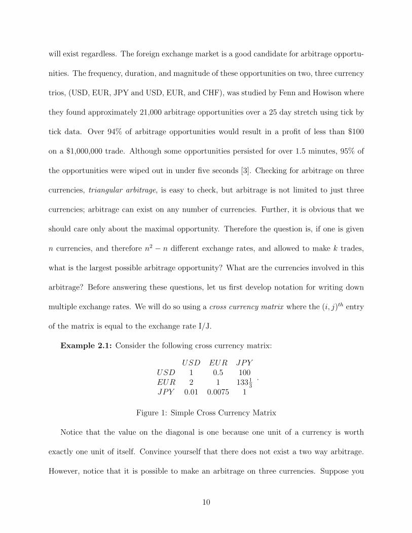
arbitrage? Before answering these questions, let us first develop notation for writing down

multiple exchange rates. We will do so using a cross currency matrix where the (i, j)th entry

of the matrix is equal to the exchange rate I/J.

Example 2.1: Consider the following cross currency matrix:

USD EUR JPYUSD 1 0.5 100EUR 2 1 1331

3

JPY 0.01 0.0075 1

.

Figure 1: Simple Cross Currency Matrix

Notice that the value on the diagonal is one because one unit of a currency is worth

exactly one unit of itself. Convince yourself that there does not exist a two way arbitrage.

However, notice that it is possible to make an arbitrage on three currencies. Suppose you

10

start by exchanging 1 USD for 100 JPY. We then exchange the 100 JPY for 0.75 EUR.

Finally, exchange the 0.75 EUR for 1.5 USD for an arbitrage profit of 0.5 USD. We are

effectively finding a series of trades such that when we multiply the exchange rates, we end

up with a value greater than one. Convince yourself that the arbitrage value is the same

regardless of where you start in the series of trades because multiplication is commutative.

We can represent this visually as:

USD → JPY → EUR→ USD

= JPY → EUR→ USD → JPY

= EUR→ USD → JPY → EUR.

The value of 1.5 can be best thought of as a multiplier, meaning that starting with X units

of the original currency will result in 1.5X units. The profit is therefore given by 1.5X-X =

0.5X.

Now let us consider this actual cross currency matrix composed of the ask prices for 5

different currencies pulled on October 25, 2016. The upper half of the matrix was taken to

be the negative of the lower half to eliminate any two way arbitrages. Notice that these are

the ask prices so we are assuming no bid-ask spread. These exchange rates were pulled at

two minute intervals, and we are assuming the listed price is the price at which we could

execute the trade, which is not always true.

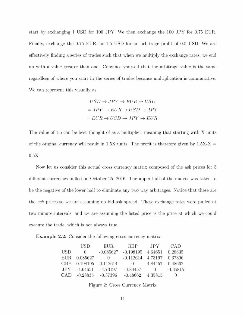
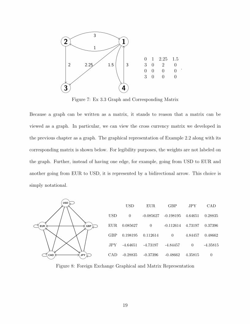
Example 2.2: Consider the following cross currency matrix:

USD EUR GBP JPY CADUSD 0 -0.085627 -0.198195 4.64651 0.28835EUR 0.085627 0 -0.112614 4.73197 0.37396GBP 0.198195 0.112614 0 4.84457 0.48662JPY -4.64651 -4.73197 -4.84457 0 -4.35815CAD -0.28835 -0.37396 -0.48662 4.35815 0

Figure 2: Cross Currency Matrix

11

This matrix is not built from the actual exchange rates themselves but rather the natural

log of the exchange rates, and therefore are slightly rounded in the matrix. We stated that

our condition for the existence of arbitrage was that there existed a series of trades such that

when the exchange rates are multiplied together we get a value greater than one and end

on the same currency we started with. If we take the natural log of the exchange rates we

can rephrase this as, “there exists an arbitrage if there exists a series of trades such that the

exchange rates, when added, sum to greater than zero and we end on the same currency we

started with.” The resulting arbitrage multiplier will be the natural log of the true arbitrage

multiplier. However, because arbitrage opportunities in the real world are on the order of

10−4, we get 1 + ln(arb.mult) ≈ arb.mult because ex ≈ 1 + x for small x.

Although this reformulation of the problem may seem trite, it will become useful when

we look to apply techniques from tropical algebra so solve the maximal-arbitrage problem.

Notice with five currencies, US dollar, euro, British pound, Japanese yen, and Canadian

dollar, we can look for arbitrage on 3, 4 and 5 currencies. Not only do we look for arbitrage,

but again, we are concerned with the maximal arbitrage. The largest triangular arbitrage is

given by the sequence

GBP → CAD → JPY → GBP.

Following this sequence will result in an arbitrage profit of 1.0002 times the amount of

pounds that you started with. Again, starting anywhere in this sequence will result in

the same multiplier. Notice that we assumed that we held a basket of all currencies and

could thus start wherever in the matrix we pleased. Our assumptions of being able to trade

instantaneously at the listed price with no transaction costs and holding all currencies is

12

closest to the position of financial institutions.

Returning to Example 2.2, the largest 4 way arbitrage is given by the sequence

GBP → CAD → USD → JPY → GBP.

Following this sequence leads to an arbitrage profit of 1.000215 times the amount of currency

that we started with. Notice that going backwards through this sequence will result in the

same arbitrage. This fact is because XY = -YX. However, swapping the positions of two

currencies in the cycle may or may not result in an arbitrage. Now let us consider if an

arbitrage on five currencies would be maximal if we are allowed to make five trades (it could

be the case that the four way arbitrage is the best we could do and our optimal 5th trade

would be no trade). Fortunately for us we do have that, given five trades, the optimal

arbitrage involves five currencies. The maximal arbitrage is given by the sequence

USD → GBP → CAD → JPY → EUR→ USD.

With this sequence we have an arbitrage multiplier of 1.00024. Notice that the magnitude

of these opportunities is quite small even without bid-ask spread considerations and thus a

large amount of capital would be required to profit. In this case, $1,000,000 USD would be

needed to make a profit of $240 USD.

If asked to find these opportunities, one might try testing every possible sequence of length

three, four, and five. This brute force method, apart from being inelegant, is inefficient. The

solution to this problem is the main focus of the paper.

13

Introduction to Graph Theory

When mathematicians wish to visually represent connections between objects, often times a

graph is used. Graph theory is a widely applicable topic studied both for its own sake and

its applicability to networks, logistics, and any subject where the system can be represented

as a collection of dots connected by lines.

[6] Definition 3.1 : A graph, G, is given by a vertex set V (G) = {v1, · · · , vn} and an

edge set E(G) = {ei,j, · · · , es,t} where em,l ∈ E(G) if and only if vm and vl are connected

with an edge.

Suppose we wish to represent four airports and the possible flights connecting them as

a graph. The vertices are our airports and an edge will connect two vertices if there is a

flight connecting them. Note that edges can be traversed in either direction, so if Dulles and

JFK are connected with an edge we can take a flight in either direction. Suppose the graph,

G, is given by V (G) = {v1, v2, v3, v4} and E(G) = {e1,2, e1,4, e1,3, e2,3}. We therefore visually

represent G by the following graph:

12

3 4

Figure 3: Simple Graph

Suppose we are concerned about the number of possible flights which connect any two air-

ports. If we allow multiple edges to connect two vertices we get a multigraph. The number

of edges connected to vertex v is known as the degree of v, written deg(v). For example, in

our example below, deg(v1) = 5.

14

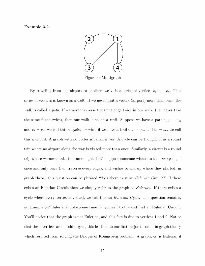
Example 3.2:

12

3 4

Figure 4: Multigraph

By traveling from one airport to another, we visit a series of vertices v1, · · · , vn. This

series of vertices is known as a walk. If we never visit a vertex (airport) more than once, the

walk is called a path. If we never traverse the same edge twice in our walk, (i.e. never take

the same flight twice), then our walk is called a trail. Suppose we have a path v1, · · · , vn

and v1 = vn, we call this a cycle; likewise, if we have a trail v1, · · · , vn and v1 = vn, we call

this a circuit. A graph with no cycles is called a tree. A cycle can be thought of as a round

trip where no airport along the way is visited more than once. Similarly, a circuit is a round

trip where we never take the same flight. Let’s suppose someone wishes to take every flight

once and only once (i.e. traverse every edge), and wishes to end up where they started, in

graph theory this question can be phrased “does there exist an Eulerian Circuit?” If there

exists an Eulerian Circuit then we simply refer to the graph as Eulerian. If there exists a

cycle where every vertex is visited, we call this an Eulerian Cycle. The question remains,

is Example 3.2 Eulerian? Take some time for yourself to try and find an Eulerian Circuit.

You’ll notice that the graph is not Eulerian, and this fact is due to vertices 1 and 2. Notice

that these vertices are of odd degree, this leads us to our first major theorem in graph theory

which resulted from solving the Bridges of Konigsberg problem. A graph, G, is Eulerian if

15

and only if every vertex is of even degree [6].

To see why this must be true, consider traversing an Eulerian Circuit. Apart from

the starting vertex, every time a vertex is entered through an edge, there must exist a

corresponding edge to exit on, therefore every vertex is of even degree. When we consider

the starting vertex, we first exit, and every other time we exit, we must have an edge to

traverse to get back to the vertex, therefore the starting vertex is also of even degree.

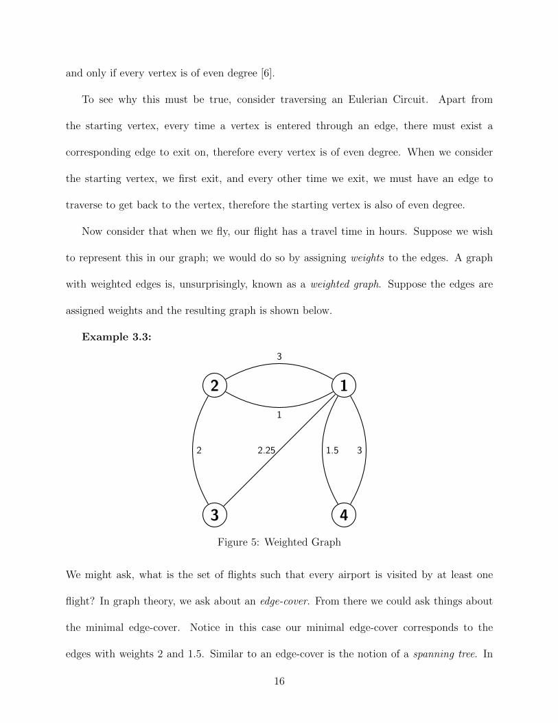
Now consider that when we fly, our flight has a travel time in hours. Suppose we wish

to represent this in our graph; we would do so by assigning weights to the edges. A graph

with weighted edges is, unsurprisingly, known as a weighted graph. Suppose the edges are

assigned weights and the resulting graph is shown below.

Example 3.3:

12

3 4

1

1.52.252

3

3

Figure 5: Weighted Graph

We might ask, what is the set of flights such that every airport is visited by at least one

flight? In graph theory, we ask about an edge-cover. From there we could ask things about

the minimal edge-cover. Notice in this case our minimal edge-cover corresponds to the

edges with weights 2 and 1.5. Similar to an edge-cover is the notion of a spanning tree. In

16

constructing a spanning tree, we look for a collection of edges such that the collection of

edges forms a tree and every vertex is included in the tree. Notice the collection of edges

with weights 1, 2.25 and 1.5 forms a spanning tree. In a tree, there must exist a path from

any vertex on the tree to any other vertex on the tree (this is not the case for an edge-

cover). One might also be concerned with the minimal spanning tree. In our example, the

minimal spanning tree would be given by the edges with weights 2, 1, and 1.5. Obviously

most examples are not this simple, and when this is the case we implement either Kruskal’s

algorithm or Prim’s algorithm to find the minimal spanning tree [2].

Suppose we want to assign every airport a call-sign and for whatever reason we want to

use as few call-signs as possible. Our only rule is that no two airports with a flight between

them are allowed to have the same call-sign. In graph theoretical terms, “call sign” is called

a color and we ask what is the minimal number of colors needed to color the graph. We

call this number the chromatic number of G. In our example, the chromatic number is three

(assign 1, 2, and 3 different colors and then assign 4 the color of either 1 or 2). In fact, for

any graph where we can write it down without edges crossing (i.e. the graph is planar), the

chromatic number is at most 4 [6]. This fact is known as the Four Color Theorem, the proof

of which took almost 200 years and remains a slightly polarizing topic in the mathematical

community. This theorem means that any map is 4-colorable and so one only needs four

different colors to assure that no two states or countries with the same color share a border.

Try and see how a map could be represented as a graph.

Now suppose each flight can only be taken in one direction. If the edges in a graph are

assigned a direction, we call the graph a digraph. Edges in these graphs can only be traversed

in their corresponding direction. If there exists a path from any vertex to any other vertex,

17

then we call the digraph strongly connected.

Example 3.4:

12

3 4

1

1.52.252

3

3

Figure 6: Weighted Digraph

We can continue to ask questions about the properties of digraphs similar to the ones we

have been asking. The topics presented were a small sampling of topics in graph theory and

the field remains an active area of research for both applied and pure mathematicians.

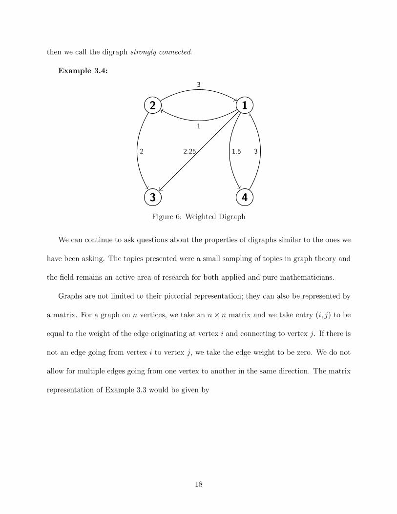
Graphs are not limited to their pictorial representation; they can also be represented by

a matrix. For a graph on n vertices, we take an n× n matrix and we take entry (i, j) to be

equal to the weight of the edge originating at vertex i and connecting to vertex j. If there is

not an edge going from vertex i to vertex j, we take the edge weight to be zero. We do not

allow for multiple edges going from one vertex to another in the same direction. The matrix

representation of Example 3.3 would be given by

18

12

3 4

1

1.52.252

3

3

0 1 2.25 1.53 0 2 00 0 0 03 0 0 0

.

Figure 7: Ex 3.3 Graph and Corresponding Matrix

Because a graph can be written as a matrix, it stands to reason that a matrix can be

viewed as a graph. In particular, we can view the cross currency matrix we developed in

the previous chapter as a graph. The graphical representation of Example 2.2 along with its

corresponding matrix is shown below. For legibility purposes, the weights are not labeled on

the graph. Further, instead of having one edge, for example, going from USD to EUR and

another going from EUR to USD, it is represented by a bidirectional arrow. This choice is

simply notational.

USD

EUR GBP

JPYCAD

USD EUR GBP JPY CAD

USD 0 -0.085627 -0.198195 4.64651 0.28835

EUR 0.085627 0 -0.112614 4.73197 0.37396

GBP 0.198195 0.112614 0 4.84457 0.48662

JPY -4.64651 -4.73197 -4.84457 0 -4.35815

CAD -0.28835 -0.37396 -0.48662 4.35815 0

Figure 8: Foreign Exchange Graphical and Matrix Representation

19

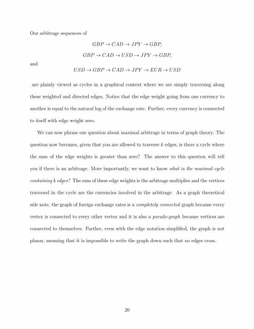
Our arbitrage sequences of

GBP → CAD → JPY → GBP,

GBP → CAD → USD → JPY → GBP,

andUSD → GBP → CAD → JPY → EUR→ USD

are plainly viewed as cycles in a graphical context where we are simply traversing along

these weighted and directed edges. Notice that the edge weight going from one currency to

another is equal to the natural log of the exchange rate. Further, every currency is connected

to itself with edge weight zero.

We can now phrase our question about maximal arbitrage in terms of graph theory. The

question now becomes, given that you are allowed to traverse k edges, is there a cycle where

the sum of the edge weights is greater than zero? The answer to this question will tell

you if there is an arbitrage. More importantly, we want to know what is the maximal cycle

containing k edges? The sum of these edge weights is the arbitrage multiplier and the vertices

traversed in the cycle are the currencies involved in the arbitrage. As a graph theoretical

side note, the graph of foreign exchange rates is a completely connected graph because every

vertex is connected to every other vertex and it is also a pseudo-graph because vertices are

connected to themselves. Further, even with the edge notation simplified, the graph is not

planar, meaning that it is impossible to write the graph down such that no edges cross.

20

Introduction to Tropical Algebra

In everyday mathematics, the ‘+’ symbol means to add two number together and the ‘×’

symbol means to multiply them. The everyday math studied by grade school students is a

special instance of what is known as a ring. They study the ring given by (R,+,×). We call

this structure a ring because addition is commutative and associative, there is an additive

identity and an additive inverse, and multiplication is associative and distributive.

However, we need not pigeonhole ourselves to the traditional definitions of addition and

multiplication to get many of these same properties. Only in the past couple decades have

mathematicians and other scientists employed what is now called the tropical approach to

mathematics. In tropical algebra, the plus symbol is taken to mean the maximum/minimum

of two numbers and the multiplication symbol is taken to mean standard addition. Typically

the symbols ⊕ and ⊗ are used to denote tropical plus and tropical times. That is, we define

a⊕ b = max{a, b} and a⊗ b = a+ b [4].

If we were to use the definitions presented, we would call this a max-plus algebra because

of our choice that a ⊕ b = max{a, b}; defining the result as a ⊕ b = min{a, b} would be

referred to as a min-plus algebra. Let us now examine the algebra to see if it can indeed be

called a ring.

Let us first mention the fact that in the max-plus world, we equip ourselves with an

additive identity, −∞, where a + −∞ = a for all a ∈ R. The additive identity further has

the property that −∞ ⊗ a = −∞. In the min-plus universe, our additive identity would

be ∞. These operators share many key properties with their standard cousins. Notice that

tropical addition is commutative over R because for every a, b in R we have that max{a, b} =

max{b, a}. It is also associative because max{max{a, b}, c} = max{max{a, c}, b}. Tropical

21

multiplication is commutative and associative over R because tropical multiplication is just

standard addition in disguise. These last properties were fairly obvious, but is it the case

that tropical multiplication distributes over tropical addition? Keep in mind that order of

operations still applies. Let us consider (a⊕ b)⊗ c. Without loss of generality, let us suppose

that a < b. Then we have

a < b ⇒ a+ c < b+ c ⇒ max{a, b}+ c = max{a+ c, b+ c}.

We therefore get that tropical multiplication is distributive (notice that the same properties

would hold in a min-plus algebra).

While so far tropical algebra has preserved several necessary ring properties, let us now

consider if there exists a additive inverse; that is, is it the case that for every element, there

is a corresponding element such that when added together we end up with the additive

identity? The answer is no; notice that minus infinity is by definition smaller than every

element and therefore can never be returned by the max function (except in the case where

all arguments are minus infinity). A similar argument holds in the min-plus case. The lack

of an additive inverse for every element precludes the algebra from being a ring and as a

consolation prize of sorts, mathematicians call such structures semi-rings. Therefore, tropical

algebra is a semi-ring given by (Rmax,⊕,⊗) where Rmax = R ∪ {−∞} [4].

Interesting to note is that in a max-plus algebra, subtraction does not exist and instead

we speak of multiplying by a negative number to accomplish the same result. Further,

polynomials become piece-wise defined. But why though do mathematicians go through the

trouble of redefining convention, and is tropical mathematics only studied and employed in

a pure math setting? As it turns out, tropical mathematics has become both a useful and

22

indeed crucial tool for areas including economics, computer science, and physics. In fact,

when the Bank of England approached renowned economist Paul Klemperer to help develop

a technique for efficiently and most beneficially auctioning off capital, the solution he came

to is entirely tropical [7][8]. Part the tropical framework’s allure is that it can allow for a

reduction in a problem’s computational complexity.

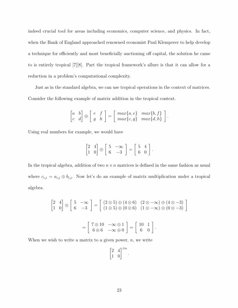
Just as in the standard algebra, we can use tropical operations in the context of matrices.

Consider the following example of matrix addition in the tropical context.

[a bc d

]⊕[e fg h

]=

[max{a, e} max{b, f}max{c, g} max{d, h}

].

Using real numbers for example, we would have

[2 41 0

]⊕[

5 −∞6 −3

]=

[5 46 0

].

In the tropical algebra, addition of two n×n matrices is defined in the same fashion as usual

where ci,j = ai,j ⊕ bi,j. Now let’s do an example of matrix multiplication under a tropical

algebra.

[2 41 0

]⊗[

5 −∞6 −3

]=

[(2⊗ 5)⊕ (4⊗ 6) (2⊗−∞)⊕ (4⊗−3)(1⊗ 5)⊕ (0⊗ 6) (1⊗−∞)⊕ (0⊗−3)

]

=

[7⊕ 10 −∞⊕ 16⊕ 6 −∞⊕ 0

]=

[10 16 0

].

When we wish to write a matrix to a given power, n, we write[2 41 0

]⊗n

.

23

Let us compute tropical powers of this matrix.[2 41 0

]⊗2

=

[2 41 0

]⊗[2 41 0

]=

[max{2 + 2, 4 + 1} max{2 + 4, 4 + 0}max{1 + 2, 0 + 1} max{1 + 4, 0 + 0}

]=

[5 63 5

].

We leave it to the reader to check that the following is correct.[2 41 0

]⊗3

=

[7 96 7

].

Tropical multiplication of a matrix by a scalar works exactly as one would think it should.

For a given real number r, we get

r ⊗[a bc d

]=

[r ⊗ a r ⊗ br ⊗ c r ⊗ d

].

In a standard algebra over Rn×n we are often concerned with finding the eigenvalues of

a matrix along with the corresponding eigenvectors.

Definition 4.1: An eigenvalue-eigenvector pair λ and x for a given matrix A satisfy the

equation Ax = λx where λ ∈ R, A ∈ Rn×n, and x ∈ Rn.

It is a reasonable question to ask if we have tropical eigenvalues and eigenvectors, and

indeed we do. First, let us think about what it would mean for a matrix to have a tropical

eigenvalue and eigenvector.

Consider the following matrix with a tropical eigenvalue and eigenvector as follows:

[a bc d

]⊗ x = λ⊗ x

where

x =

[rs

].

24

It follows then that [a bc d

]⊗[rs

]= λ⊗

[rs

].

Therefore, if we were to write this in a standard algebra, we would find

[max{a+ r, b+ s}max{c+ r, d+ s}

]=

[r + λs+ λ

].

It is now clear that r, s and λ must satisfy the conditions that max{a + r, b + s} = r + λ

and max{c+ r, d+ s} = s+λ. Eigenvector-eigenvalue pairs are widely applicable and useful

for repeatedly multiplying by a matrix. We now know what it would mean for tropical

eigenvalues and eigenvectors to exist, but the question remains, how does one find them?

The problem of trying to find a tropical eigenvalue for some matrix A is equivalent to

trying to find the maximal normalized weight across all cycles in the graphical representation

(G(A)), assuming that the graph is strongly connected. We define the normalized weight of

a cycle to be the sum of the edge weights involved in a cycle divided by the number of edges.

[5] Theorem 4.1: If A ∈ Rn×n with G(A) strongly connected, then A has a unique

tropical eigenvalue equal to the maximal normalized weight across all directed cycles in G(A).

We do not, however, need to check very possible cycle in the graph. In 1978, Richard

Karp published an algorithm for finding the maximal normalized weight across all cycles.

Before showing Karp’s algorithm, we note that the identity matrix in the max-plus tropical

algebra, B, where bij = 0 if i = j and −∞ otherwise. Now we are ready for Karp’s algorithm

[1][9]:

• For A ∈ Rn×n arbitrarily choose some column, bj, of the n × n identity matrix; set

bj = v(0).

25

• Compute v(k) = A⊗ v(k − 1) for k = 1, 2, · · · , n

• Compute λ = maxi=1,··· ,n

[mink=0,··· ,n−1

[vi(n)−vi(k)

n−k

]]Before progressing through our foreign exchange example, let us revisit our favorite net-

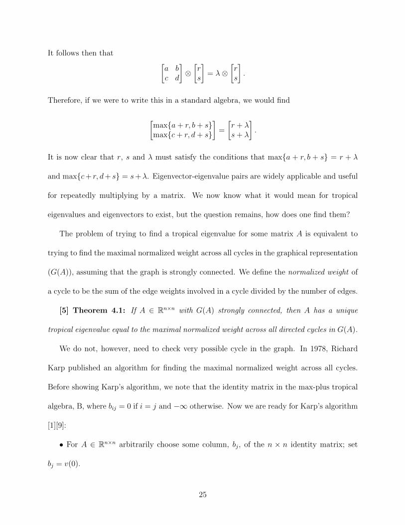
work of airports and see how Karp’s algorithm would be implemented. Because we require

our graph be strongly connected, we have to add a route going from 3. Let’s choose it to

have weight -4 and to travel to airport 4.

12

3 4

1

1.52.252

3

-4

3−∞ 1 2.25 1.5

3 −∞ 2 −∞−∞ −∞ −∞ -4

3 −∞ −∞ −∞

Figure 9: Weighted Digraph and Tropical Matrix Representation

Take note that in a tropical algebra, instead of taking an edge weight to be zero between

to vertices if there does not exist an edge, we take the edge weight to be −∞, the additive

identity under a tropical algebra. Let’s implement Karp’s algorithm and let’s arbitrarily take

our v(0) to be the 3rd column in the identity matrix. Our first step is therefore:

v(1) = A⊗ v(0) =

−∞ 1 2.25 1.5

3 −∞ 2 −∞−∞ −∞ −∞ −4

3 −∞ −∞ −∞

⊗−∞−∞

0

−∞

=

26

(−∞⊗−∞)⊕ (1⊗−∞)⊕ (2.25⊗ 0)⊕ (1.5⊗−∞)

(3⊗−∞)⊕ (−∞⊗−∞)⊕ (2⊗ 0)⊕ (−∞⊗−∞)

(−∞⊗−∞)⊕ (−∞⊗−∞)⊕ (−∞⊗ 0)⊕ (−4⊗−∞)

(3⊗−∞)⊕ (−∞⊗−∞)⊕ (−∞⊗ 0)⊕ (−∞⊗−∞)

=

2.25

2

−∞−∞

It should not be surprising that by multiplying by the 3rd column of the identity matrix, we

find ourselves left with the 3rd column of A. Notice, this column of A represents all possible

paths of length 1 that lead to vertex 3.

v(2) = A⊗ v(1) =

−∞ 1 2.25 1.5

3 −∞ 2 −∞−∞ −∞ −∞ −4

3 −∞ −∞ −∞

⊗

2.25

2

−∞−∞

=

(−∞⊗ 2.25)⊕ (1⊗ 2)⊕ (2.25⊗−∞)⊕ (1.5⊗−∞)

(3⊗ 2.25)⊕ (−∞⊗ 2)⊕ (2⊗−∞)⊕ (−∞⊗−∞)

(−∞⊗ 2.25)⊕ (−∞⊗ 2)⊕ (−∞⊗−∞)⊕ (−4⊗−∞)

(3⊗ 2.25)⊕ (−∞⊗ 2)⊕ (−∞⊗−∞)⊕ (−∞⊗−∞)

=

3

5.25

−∞5.25

Notice the nth row of this vector is the maximal weight path of length two starting at vertex

n and finishing at vertex 3. For the penultimate iteration, we find

v(3) = A⊗ v(2) =

−∞ 1 2.25 1.5

3 −∞ 2 −∞−∞ −∞ −∞ −4

3 −∞ −∞ −∞

⊗

3

5.25

−∞5.25

=

(−∞⊗ 3)⊕ (1⊗ 5.25)⊕ (2.25⊗−∞)⊕ (1.5⊗ 5.25)

(3⊗ 3)⊕ (−∞⊗ 5.25)⊕ (2⊗−∞)⊕ (−∞⊗ 5.25)

(−∞⊗ 3)⊕ (−∞⊗ 5.25)⊕ (−∞⊗−∞)⊕ (−4⊗ 5.25)

(3⊗ 3)⊕ (−∞⊗ 5.25)⊕ (−∞⊗−∞)⊕ (−∞⊗ 5.25)

=

max{6.25, 6.75}

6

1.25

6

.

At this stage, let’s more closely examine what exactly the algorithm is doing. Notice that we

are choosing the maximum between 6.25 and 6.75. These weights correspond to the options

of traveling 1→ 2→ 1→ 3 or going 1→ 4→ 1→ 3. Our second entry has gone from 5.25

27

to 6 because now instead of going 4 → 1 → 3 we can travel 4 → 1 → 2 → 3. Because we

now have paths of length three, we are able to start and end at 3 by going 3→ 4→ 1→ 3.

For the last iteration, we find

v(4) = A⊗ v(3) =

−∞ 1 2.25 1.5

3 −∞ 2 −∞−∞ −∞ −∞ −4

3 −∞ −∞ −∞

⊗

6.75

6

1.25

6

=

(−∞⊗ 6.75)⊕ (1⊗ 6)⊕ (2.25⊗ 1.25)⊕ (1.5⊗ 6)

(3⊗ 6.75)⊕ (−∞⊗ 6)⊕ (2⊗ 1.25)⊕ (−∞⊗ 6)

(−∞⊗ 6.75)⊕ (−∞⊗ 6)⊕ (−∞⊗ 1.25)⊕ (−4⊗ 6)

(3⊗ 6.75)⊕ (−∞⊗ 6)⊕ (−∞⊗ 1.25)⊕ (−∞⊗ 6)

=

7.5

9.75

2

9.75

.Let us now write down again all of the v(k)’s.

v(0) =

−∞−∞

0−∞

; v(1) =

2.25

2−∞−∞

; v(2) =

3

5.25−∞5.25

; v(3) =

6.75

61.25

6

; v(4) =

7.59.75

29.75

.The final part of the algorithm is to choose the maximum of the following minimums.

min

[7.5 +∞

4− 0,7.5− 2.25

4− 1,7.5− 3

4− 2,7.5− 6.75

4− 3

]= .75

min

[9.75 +∞

4− 0,9.75− 2

4− 1,9.75− 5.25

4− 2,9.75− 6

4− 3

]= 2.25

min

[2− 0

4− 0,2 +∞4− 1

,2 +∞4− 2

,2− 1.25

4− 3

]= .5

min

[9.75 +∞

4− 0,9.75 +∞

4− 1,9.75− 5.25

4− 2,9.75− 6

4− 3

]= 2.25.

The maximum of these values is of course 2.25. The claim, then, is that 2.25 is the maximal

normalized weight across all cycles in G and is also the eigenvalue for its matrix. Looking at

28

G again, we can see it is obvious that traversing the cycle between vertices 1 and 4 will give

us the largest “weight-bang” for our “edge-traversing-buck” and that the normalized weight

is 2.25.

12

3 4

1

1.52.252

3

-4

3

Now consider if we were to implement Karp’s algorithm on a matrix of foreign exchange

rates. We would be given the maximal normalized cycle weight. Meaning, Karp’s algorithm

can tell us the maximal (average) arbitrage multiplier per trade. However, it does not tell

us the vertices involved in this cycle. Further, the number is the maximal average arbitrage

per trade and thus we are unsure of our maximal arbitrage value; it may be a multiple of

the number produced by Karp’s algorithm, or it could be an entirely different number. One

can easily imagine a scenario where the maximal arbitrage per trade is on a cycle of length

three but the maximal arbitrage possible is on a cycle of length four. With which should we

concern ourselves? That question aside, it remains to be answered, how do we detect the

largest arbitrage possible? Again, we look to tropical algebra.

Theorem 4.2: Given a matrix, A ∈ Rn×nmax , the maximal path weight of length k in G(A)

going from vertex i to vertex j is given by a⊗ki,j where A⊗k is the kth tropical power of A.

Proof: We proceed by induction on k. The first power is trivial so let us take k = 2 as

our base case. By definition, a⊗2i,j = maxm=1,··· ,n{ai,m+am,j}. Notice that the set of all possible

29

paths of length two is given by {ai → am → aj} for m = 1, · · · , n. The set of all length two

path weights would therefore be given by {ai,m+am,j} for m = 1, · · · , n. Therefore a⊗2i,j is the

maximal length two path weight. Now assume that up to k = N , a⊗ki,j is the maximal path

weight of length k going from vertex i to j. By definition, a⊗Ni,j = maxm=1,··· ,n{a⊗N−1

i,m +am,j}.

By the induction hypothesis, a⊗N−1i,m is the maximal path weight of length N − 1 going from

vertex i to vertex m. Let us just consider the N − 1 steps in the maximal path before

we travel to vertex j; we finish this path on some m∗ and from there, we travel to j. If

the path on which we traveled to m∗ was not maximal and was of weight ω, then we could

instead travel the path of weight a⊗N−1i,m∗ and our new path would be of greater weight because

a⊗N−1i,m∗ + am∗,j > ω + am∗,j. Therefore we only need to consider the maximal paths of length

N − 1 leading up to our final edge traversing. The possible path weights are therefore given

by the set {a⊗N−1i,m + am,j} for m = 1, · · · , n. Therefore, by definition, a⊗N

i,j is the maximal

path weight of length N going from vertex i to vertex j. �

Before presenting the corollary to this theorem, which is our main result, let us return

to our arbitrage example given by the following graph and corresponding matrix.

USD

EUR GBP

JPYCAD

USD EUR GBP JPY CAD

USD 0 -0.08556 -0.1981 4.6470 0.2886

EUR 0.08563 0 -0.1124 4.7322 0.3741

GBP 0.1982 0.1126 0 4.8450 0.4867

JPY -4.6465 -4.7320 -4.8446 0 -4.3581

CAD -0.2884 -0.3740 -0.4866 4.3582 0

.

30

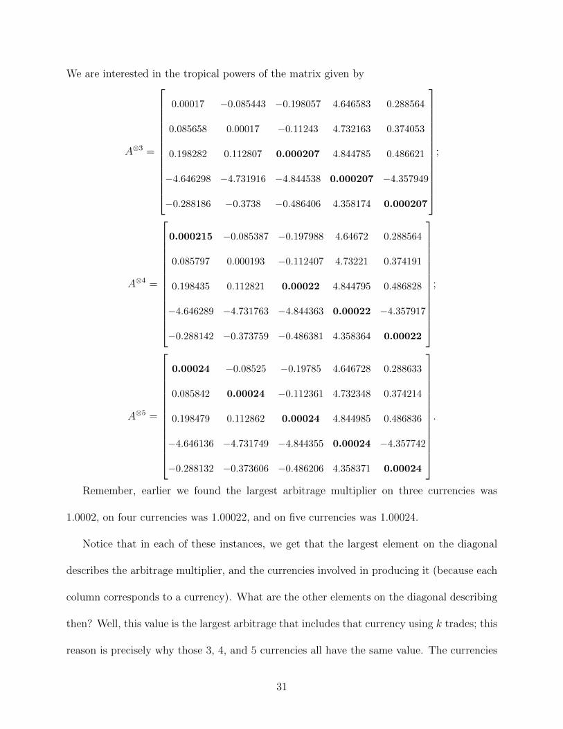
We are interested in the tropical powers of the matrix given by

A⊗3 =

0.00017 −0.085443 −0.198057 4.646583 0.288564

0.085658 0.00017 −0.11243 4.732163 0.374053

0.198282 0.112807 0.000207 4.844785 0.486621

−4.646298 −4.731916 −4.844538 0.000207 −4.357949

−0.288186 −0.3738 −0.486406 4.358174 0.000207

;

A⊗4 =

0.000215 −0.085387 −0.197988 4.64672 0.288564

0.085797 0.000193 −0.112407 4.73221 0.374191

0.198435 0.112821 0.00022 4.844795 0.486828

−4.646289 −4.731763 −4.844363 0.00022 −4.357917

−0.288142 −0.373759 −0.486381 4.358364 0.00022

;

A⊗5 =

0.00024 −0.08525 −0.19785 4.646728 0.288633

0.085842 0.00024 −0.112361 4.732348 0.374214

0.198479 0.112862 0.00024 4.844985 0.486836

−4.646136 −4.731749 −4.844355 0.00024 −4.357742

−0.288132 −0.373606 −0.486206 4.358371 0.00024

.

Remember, earlier we found the largest arbitrage multiplier on three currencies was

1.0002, on four currencies was 1.00022, and on five currencies was 1.00024.

Notice that in each of these instances, we get that the largest element on the diagonal

describes the arbitrage multiplier, and the currencies involved in producing it (because each

column corresponds to a currency). What are the other elements on the diagonal describing

then? Well, this value is the largest arbitrage that includes that currency using k trades; this

reason is precisely why those 3, 4, and 5 currencies all have the same value. The currencies

31

are all involved in the maximal cycle and thus it must be that case that the maximal cycle

they are involved in has the same weight for each of them.

How do these values relate the Karp’s algorithm? If these are all maximal arbitrages,

and Karp’s algorithm produces only one number, then how can both be correct? Remember,

Karp’s algorithm is concerned with the maximal normalized cycle weight, not the maximal

possible cycle weight. If we implement Karp’s algorithm, we find it returns a value of

0.000069. We now note, that

0.000207

3= 0.000069,

0.000215

4= 0.000054,

0.00024

5= 0.000048.

Karp’s algorithm has served us well and has indeed found the cycle with the largest nor-

malized weight, across all possible cycle lengths (we exclude cycles of length two because, as

mentioned before, there does not exist a two way arbitrage).

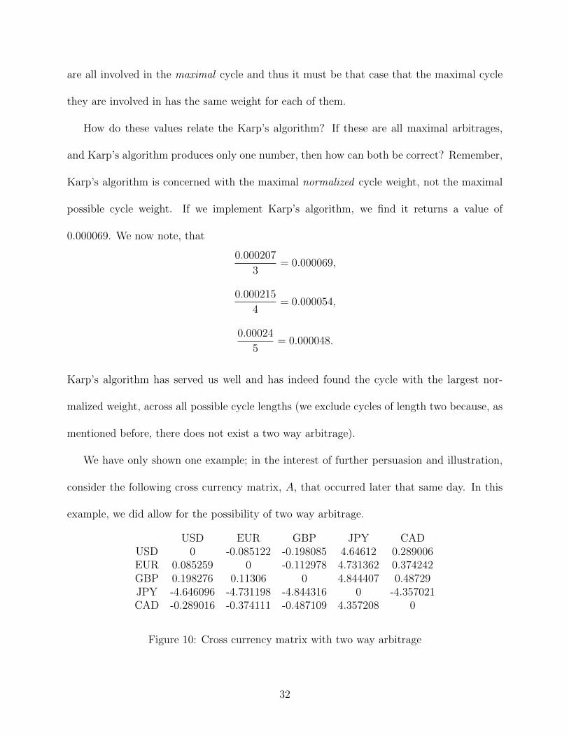
We have only shown one example; in the interest of further persuasion and illustration,

consider the following cross currency matrix, A, that occurred later that same day. In this

example, we did allow for the possibility of two way arbitrage.

USD EUR GBP JPY CADUSD 0 -0.085122 -0.198085 4.64612 0.289006EUR 0.085259 0 -0.112978 4.731362 0.374242GBP 0.198276 0.11306 0 4.844407 0.48729JPY -4.646096 -4.731198 -4.844316 0 -4.357021CAD -0.289016 -0.374111 -0.487109 4.357208 0

Figure 10: Cross currency matrix with two way arbitrage

32

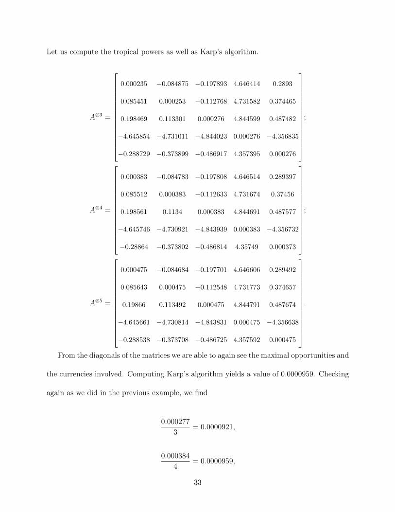
Let us compute the tropical powers as well as Karp’s algorithm.

A⊗3 =

0.000235 −0.084875 −0.197893 4.646414 0.2893

0.085451 0.000253 −0.112768 4.731582 0.374465

0.198469 0.113301 0.000276 4.844599 0.487482

−4.645854 −4.731011 −4.844023 0.000276 −4.356835

−0.288729 −0.373899 −0.486917 4.357395 0.000276

;

A⊗4 =

0.000383 −0.084783 −0.197808 4.646514 0.289397

0.085512 0.000383 −0.112633 4.731674 0.37456

0.198561 0.1134 0.000383 4.844691 0.487577

−4.645746 −4.730921 −4.843939 0.000383 −4.356732

−0.28864 −0.373802 −0.486814 4.35749 0.000373

;

A⊗5 =

0.000475 −0.084684 −0.197701 4.646606 0.289492

0.085643 0.000475 −0.112548 4.731773 0.374657

0.19866 0.113492 0.000475 4.844791 0.487674

−4.645661 −4.730814 −4.843831 0.000475 −4.356638

−0.288538 −0.373708 −0.486725 4.357592 0.000475

.

From the diagonals of the matrices we are able to again see the maximal opportunities and

the currencies involved. Computing Karp’s algorithm yields a value of 0.0000959. Checking

again as we did in the previous example, we find

0.000277

3= 0.0000921,

0.000384

4= 0.0000959,

33

0.000475

5= 0.0000951.

Again, Karp’s algorithm agrees with our results from taking the matrix to different tropical

powers. Now, let us examine the following corollaries to Theorem 4.2.

Corollary 4.3: Given a cross-currency matrix with n currencies, the maximal arbitrage

using k trades and involving currency i is given by a⊗ki,i .

Corollary 4.4: Given a cross-currency matrix with n currencies, the maximal arbitrage

using k trades is given by maxl=1,··· ,n{a⊗kl,l }. If k distinct currencies c1, c2, · · · , ck are involved

in the maximal cycle then a⊗kc1,c1

= a⊗kc2,c2

= · · · = a⊗kck,ck

.

To see why Corollary 4.3 falls out from Theorem 4.2, consider that when we examine a⊗ki,i

we are getting the maximal value of a path starting and ending at currency i; paths that

start and end on the same nodes are, by definition, cycles. Further, because the cycle weights

are foreign exchange rates, we interpret a positive cycle weight as an arbitrage. Corollary

4.4 is immediate from Corollary 4.3.

In our example with no two way arbitrage, we saw that the maximal normalized cycle

weight decreased as the cycles got longer. For our example with two way arbitrage, this fact

was not true. This observation begs the question, is it ever the case that we could have tiny

arbitrage values for short cycles and considerably larger arbitrage values for longer cycles,

all in an environment with no two way arbitrage?

In the next chapter, we show the results of simulating 40,000 possible changes to the

currency matrix and produce instances in which there was no two way arbitrage, and the

longer cycle arbitrages were considerably larger than the triangular arbitrage.

34

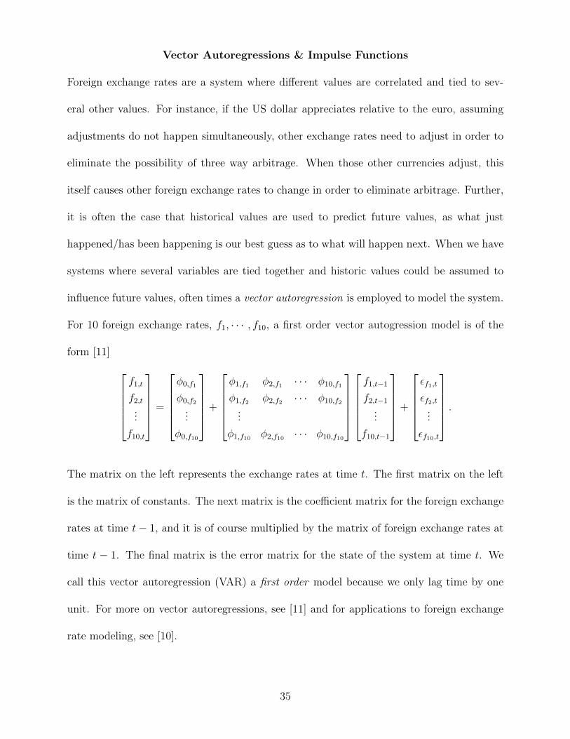
Vector Autoregressions & Impulse Functions

Foreign exchange rates are a system where different values are correlated and tied to sev-

eral other values. For instance, if the US dollar appreciates relative to the euro, assuming

adjustments do not happen simultaneously, other exchange rates need to adjust in order to

eliminate the possibility of three way arbitrage. When those other currencies adjust, this

itself causes other foreign exchange rates to change in order to eliminate arbitrage. Further,

it is often the case that historical values are used to predict future values, as what just

happened/has been happening is our best guess as to what will happen next. When we have

systems where several variables are tied together and historic values could be assumed to

influence future values, often times a vector autoregression is employed to model the system.

For 10 foreign exchange rates, f1, · · · , f10, a first order vector autogression model is of the

form [11] f1,t

f2,t...

f10,t

=

φ0,f1

φ0,f2...

φ0,f10

+

φ1,f1 φ2,f1 · · · φ10,f1

φ1,f2 φ2,f2 · · · φ10,f2...

φ1,f10 φ2,f10 · · · φ10,f10

f1,t−1

f2,t−1

...

f10,t−1

+

εf1,t

εf2,t...

εf10,t

.

The matrix on the left represents the exchange rates at time t. The first matrix on the left

is the matrix of constants. The next matrix is the coefficient matrix for the foreign exchange

rates at time t− 1, and it is of course multiplied by the matrix of foreign exchange rates at

time t − 1. The final matrix is the error matrix for the state of the system at time t. We

call this vector autoregression (VAR) a first order model because we only lag time by one

unit. For more on vector autoregressions, see [11] and for applications to foreign exchange

rate modeling, see [10].

35

Once a VAR model is generated, an impulse response function can be used to see how

the system is predicted to change through time given a one standard deviation “shock” to

the error term of one of the variables [11]. VAR models and impulse functions are powerful

tools in time series, however, because we simply need to them to see many different ways in

which the system could plausibly change, we will not delve into the more technical aspects.

We estimated a VAR model where we assumed the USDEUR exchange rate was the main

driver; a shock to this major currency pair would likely have a strong effect on the others.

In our model, we included nine other exchange rates. We only needed nine because if we

assume no two way arbitrage, then the change to XY will be exactly -YX (because we have

taken the natural log of exchange rates). Therefore, because XY and YX vary linearly with

each other, one was excluded due to multicollinearity concerns. From there, a fifth order

VAR model was estimated and a shock to the USDEUR exchange rate was simulated by an

impulse response function. The impulse response function returned the estimated change in

the other foreign exchange rates.

Because a VAR model is linear, the responses to a shock will scale as the shock itself is

scaled. After we estimated the impulse function, we scaled the shock (and the responses to it)

40,000 different times by multiplying the shock and responses by the same random variable

with mean one and standard deviation four. The scaling factor was randomly multiplied by

either one or negative one. Then, the responses in the different currency pairs were allowed

to “wiggle.” By wiggle, we mean to say that the change in, for instance, JPYCAD, was taken

to be the predicted change (including the scaling factor) times z where z was distributed

normally with mean 1 and standard deviation 1. Note that a different z value was generated

for each simulation and each currency pair was multiplied by its own z.

36

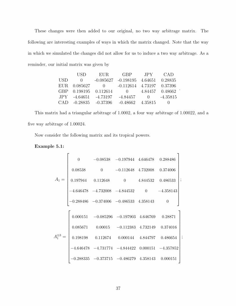
These changes were then added to our original, no two way arbitrage matrix. The

following are interesting examples of ways in which the matrix changed. Note that the way

in which we simulated the changes did not allow for us to induce a two way arbitrage. As a

reminder, our initial matrix was given by

USD EUR GBP JPY CADUSD 0 -0.085627 -0.198195 4.64651 0.28835EUR 0.085627 0 -0.112614 4.73197 0.37396GBP 0.198195 0.112614 0 4.84457 0.48662JPY -4.64651 -4.73197 -4.84457 0 -4.35815CAD -0.28835 -0.37396 -0.48662 4.35815 0

.

This matrix had a triangular arbitrage of 1.0002, a four way arbitrage of 1.00022, and a

five way arbitrage of 1.00024.

Now consider the following matrix and its tropical powers.

Example 5.1:

A1 =

0 −0.08538 −0.197944 4.646478 0.288486

0.08538 0 −0.112648 4.732008 0.374006

0.197944 0.112648 0 4.844532 0.486533

−4.646478 −4.732008 −4.844532 0 −4.358143

−0.288486 −0.374006 −0.486533 4.358143 0

;

A⊗31 =

0.000151 −0.085296 −0.197903 4.646769 0.28871

0.085671 0.00015 −0.112383 4.732149 0.374016

0.198198 0.112674 0.000144 4.844797 0.486654

−4.646478 −4.731774 −4.844422 0.000151 −4.357852

−0.288335 −0.373715 −0.486279 4.358143 0.000151

;

37

A⊗41 =

0.000291 −0.085229 −0.197763 4.646853 0.28871

0.085671 0.000291 −0.112273 4.732159 0.374157

0.198319 0.112818 0.000265 4.844797 0.486684

−4.646327 −4.731774 −4.844381 0.000291 −4.357768

−0.288335 −0.373631 −0.486279 4.358294 0.000291

;

A⊗51 =

0.000375 −0.085089 −0.197653 4.646853 0.288777

0.085681 0.000375 −0.112273 4.7323 0.374297

0.198319 0.112939 0.000375 4.844827 0.486824

−4.646187 −4.731707 −4.844241 0.000375 −4.357768

−0.288184 −0.373631 −0.486238 4.358434 0.000375

.

As can be seen from the tropical powers, the arbitrage on three currencies is much smaller

than the arbitrage on five currencies. The following example is another case in which the

longer cycle arbitrages were significantly higher than the three cycle.

Example 5.2:

A2 =

0 −0.085911 −0.19868 4.646175 0.288121

0.085911 0 −0.112544 4.731885 0.37393

0.19868 0.112544 0 4.844643 0.486683

−4.646175 −4.731885 −4.844643 0 −4.358161

−0.288121 −0.37393 −0.486683 4.358161 0

;

38

A⊗32 =

0.000225 −0.085603 −0.198254 4.646282 0.288228

0.086136 0.000225 −0.112544 4.732311 0.374257

0.19868 0.11297 0.000225 4.844962 0.486801

−4.645749 −4.731874 −4.844429 0.000214 −4.357746

−0.287794 −0.373724 −0.486268 4.358172 0.000209

;

A⊗42 =

0.000426 −0.085603 −0.198147 4.6464 0.288429

0.086136 0.000426 −0.112319 4.732418 0.374257

0.198905 0.113077 0.000426 4.844962 0.486908

−4.645749 −4.73166 −4.844418 0.000426 −4.357628

−0.287588 −0.373705 −0.486268 4.358381 0.000415

;

A⊗52 =

0.000533 −0.085485 −0.198147 4.646601 0.288547

0.086361 0.000533 −0.112118 4.732418 0.374364

0.199106 0.113077 0.000533 4.84508 0.487109

−4.645738 −4.731459 −4.844204 0.000533 −4.357628

−0.287588 −0.373499 −0.486249 4.358587 0.000533

.

The following is an example where all arbitrage values were quite low.

Example 5.3:

A3 =

0 −0.085259 −0.19786 4.646736 0.288695

0.085259 0 −0.112488 4.732034 0.373987

0.19786 0.112488 0 4.844524 0.486518

−4.646736 −4.732034 −4.844524 0 −4.358129

−0.288695 −0.373987 −0.486518 4.358129 0

;

39

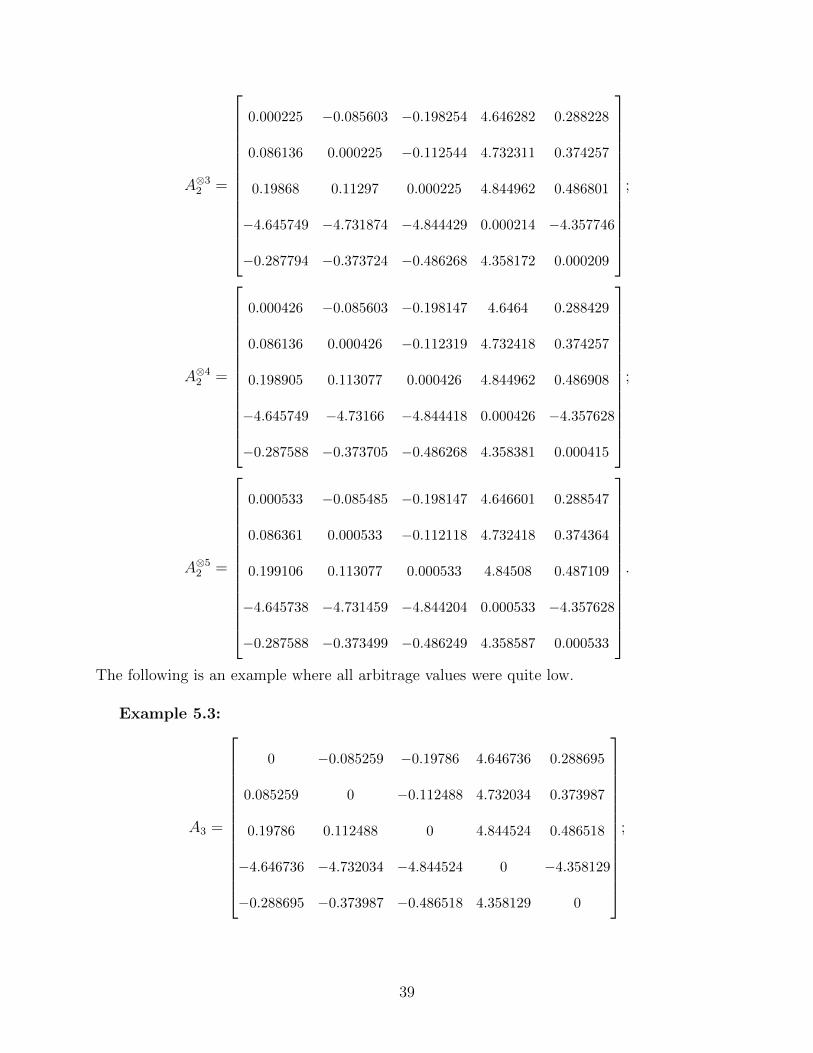
A⊗33 =

0.000113 −0.08521 −0.1977 4.646857 0.288771

0.08538 0.000113 −0.112408 4.732159 0.374067

0.197911 0.112613 0.000123 4.844684 0.486588

−4.646662 −4.731923 −4.844483 0.000123 −4.357969

−0.288535 −0.373866 −0.486393 4.358129 0.000123

;

A⊗43 =

0.00016 −0.085146 −0.197667 4.6469 0.288818

0.085452 0.000125 −0.112365 4.732196 0.37411

0.197983 0.112652 0.00016 4.844717 0.486641

−4.646613 −4.731911 −4.844401 0.00016 −4.357936

−0.288533 −0.373794 −0.486354 4.358252 0.00016

;

A⊗53 =

0.000193 −0.085099 −0.197624 4.646947 0.288855

0.085495 0.000193 −0.112328 4.732239 0.374153

0.19802 0.112724 0.000193 4.84477 0.486678

−4.646541 −4.731872 −4.844364 0.000193 −4.357883

−0.288484 −0.373782 −0.486272 4.358289 0.000193

.

The instance in which the five way arbitrage was highest relative to the lower cycles is given

by the following matrix.

Example 5.4:

A4 =

0 −0.085772 −0.198271 4.64635 0.288199

0.085772 0 −0.112732 4.731907 0.373953

0.198271 0.112732 0 4.844615 0.486665

−4.64635 −4.731907 −4.844615 0 −4.358154

−0.288199 −0.373953 −0.486665 4.358154 0

;

40

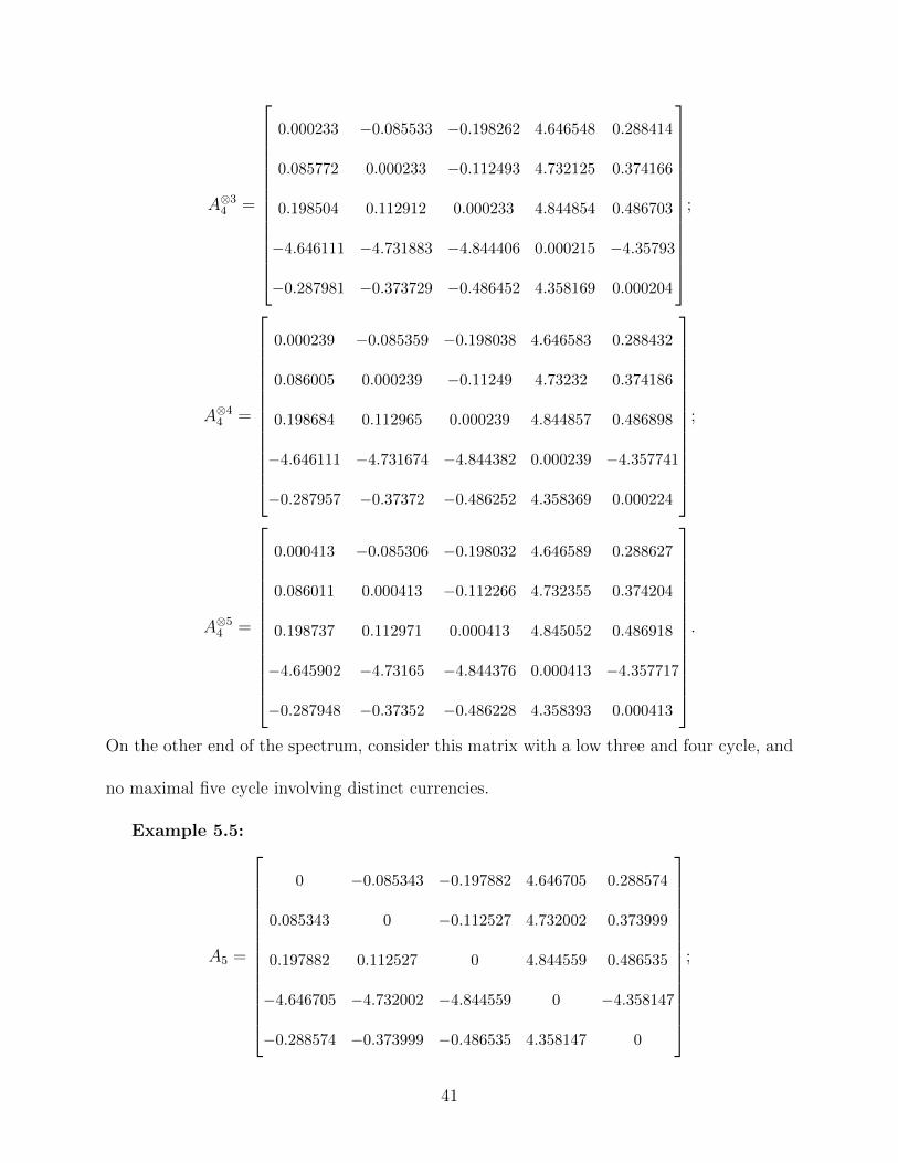
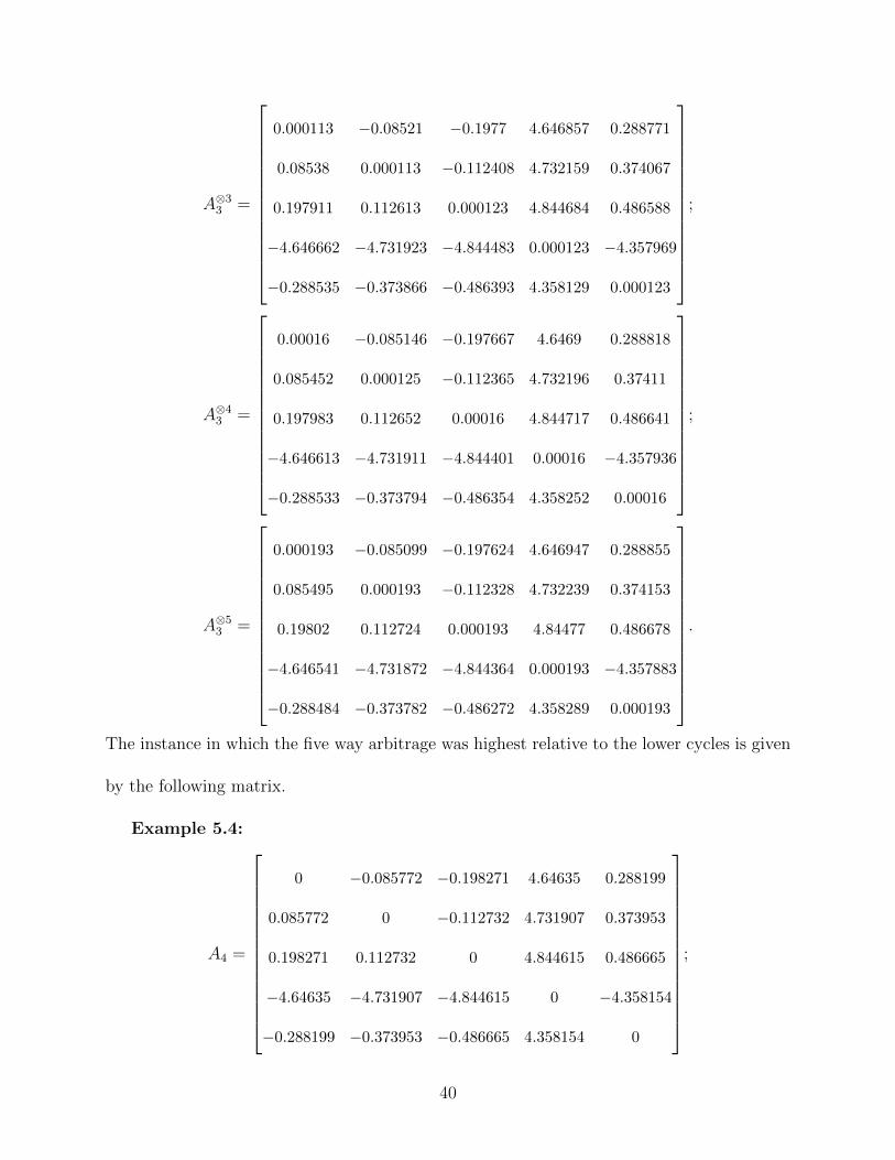
A⊗34 =

0.000233 −0.085533 −0.198262 4.646548 0.288414

0.085772 0.000233 −0.112493 4.732125 0.374166

0.198504 0.112912 0.000233 4.844854 0.486703

−4.646111 −4.731883 −4.844406 0.000215 −4.35793

−0.287981 −0.373729 −0.486452 4.358169 0.000204

;

A⊗44 =

0.000239 −0.085359 −0.198038 4.646583 0.288432

0.086005 0.000239 −0.11249 4.73232 0.374186

0.198684 0.112965 0.000239 4.844857 0.486898

−4.646111 −4.731674 −4.844382 0.000239 −4.357741

−0.287957 −0.37372 −0.486252 4.358369 0.000224

;

A⊗54 =

0.000413 −0.085306 −0.198032 4.646589 0.288627

0.086011 0.000413 −0.112266 4.732355 0.374204

0.198737 0.112971 0.000413 4.845052 0.486918

−4.645902 −4.73165 −4.844376 0.000413 −4.357717

−0.287948 −0.37352 −0.486228 4.358393 0.000413

.

On the other end of the spectrum, consider this matrix with a low three and four cycle, and

no maximal five cycle involving distinct currencies.

Example 5.5:

A5 =

0 −0.085343 −0.197882 4.646705 0.288574

0.085343 0 −0.112527 4.732002 0.373999

0.197882 0.112527 0 4.844559 0.486535

−4.646705 −4.732002 −4.844559 0 −4.358147

−0.288574 −0.373999 −0.486535 4.358147 0

;

41

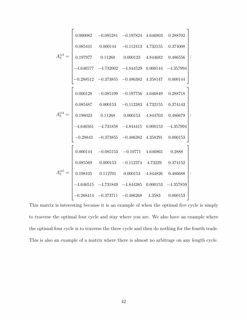
A⊗35 =

0.000082 −0.085281 −0.197824 4.646803 0.288702

0.085441 0.000144 −0.112413 4.732155 0.374008

0.197977 0.11268 0.000123 4.844682 0.486556

−4.646577 −4.732002 −4.844529 0.000144 −4.357994

−0.288512 −0.373855 −0.486382 4.358147 0.000144

;

A⊗45 =

0.000128 −0.085199 −0.197756 4.646849 0.288718

0.085487 0.000153 −0.112383 4.732155 0.374143

0.198023 0.11268 0.000153 4.844703 0.486679

−4.646561 −4.731858 −4.844415 0.000153 −4.357994

−0.28843 −0.373855 −0.486382 4.358291 0.000153

;

A⊗55 =

0.000144 −0.085153 −0.19771 4.646865 0.2888

0.085569 0.000153 −0.112374 4.73229 0.374152

0.198105 0.112701 0.000153 4.844826 0.486688

−4.646515 −4.731849 −4.844385 0.000153 −4.357859

−0.288414 −0.373711 −0.486268 4.3583 0.000153

.

This matrix is interesting because it is an example of when the optimal five cycle is simply

to traverse the optimal four cycle and stay where you are. We also have an example where

the optimal four cycle is to traverse the three cycle and then do nothing for the fourth trade.

This is also an example of a matrix where there is almost no arbitrage on any length cycle.

42

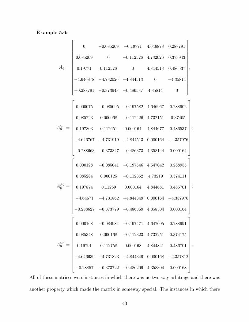
Example 5.6:

A6 =

0 −0.085209 −0.19771 4.646878 0.288791

0.085209 0 −0.112526 4.732026 0.373943

0.19771 0.112526 0 4.844513 0.486537

−4.646878 −4.732026 −4.844513 0 −4.35814

−0.288791 −0.373943 −0.486537 4.35814 0

;

A⊗36 =

0.000075 −0.085095 −0.197582 4.646967 0.288902

0.085223 0.000068 −0.112426 4.732151 0.37405

0.197803 0.112651 0.000164 4.844677 0.486537

−4.646767 −4.731919 −4.844513 0.000164 −4.357976

−0.288663 −0.373847 −0.486373 4.358144 0.000164

;

A⊗46 =

0.000128 −0.085041 −0.197546 4.647042 0.288955

0.085284 0.000125 −0.112362 4.73219 0.374111

0.197874 0.11269 0.000164 4.844681 0.486701

−4.64671 −4.731862 −4.844349 0.000164 −4.357976

−0.288627 −0.373779 −0.486369 4.358304 0.000164

;

A⊗56 =

0.000168 −0.084984 −0.197471 4.647095 0.288991

0.085348 0.000168 −0.112323 4.732251 0.374175

0.19791 0.112758 0.000168 4.844841 0.486701

−4.646639 −4.731823 −4.844349 0.000168 −4.357812

−0.28857 −0.373722 −0.486209 4.358304 0.000168

.

All of these matrices were instances in which there was no two way arbitrage and there was

another property which made the matrix in someway special. The instances in which there

43

was a high five way arbitrage relative to three way and four way suggests that even if there

is no three way arbitrage (either because it simply does not exist or because transaction

costs would eliminate it), a profitable five way arbitrage could still exist. These instances,

however, are likely extremely rare. Even with 40,000 simulations, the percent of arbitrage

instances where the the five way arbitrage was at least two times greater than the three way

arbitrage was only 1.3%.

Finally, here is an example where the arbitrage on three currencies may have been elim-

inated by transaction costs, but the arbitrage on five currencies was of a high magnitude.

Example 5.7:

A7 =

0 −0.08624 −0.198427 4.645719 0.287863

0.08624 0 −0.112718 4.731631 0.373965

0.198427 0.112718 0 4.844671 0.486787

−4.645719 −4.731631 −4.844671 0 −4.358174

−0.287863 −0.373965 −0.486787 4.358174 0

;

A⊗37 =

0.000531 −0.085387 −0.198427 4.646534 0.28836

0.08642 0.000531 −0.112187 4.732484 0.3746

0.19928 0.11333 0.000531 4.844961 0.487005

−4.645391 −4.731428 −4.843818 0.000525 −4.357359

−0.287217 −0.373457 −0.485972 4.358381 0.000508

;

44

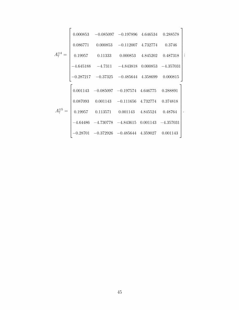
A⊗47 =

0.000853 −0.085097 −0.197896 4.646534 0.288578

0.086771 0.000853 −0.112007 4.732774 0.3746

0.19957 0.11333 0.000853 4.845202 0.487318

−4.645188 −4.7311 −4.843818 0.000853 −4.357031

−0.287217 −0.37325 −0.485644 4.358699 0.000815

;

A⊗57 =

0.001143 −0.085097 −0.197574 4.646775 0.288891

0.087093 0.001143 −0.111656 4.732774 0.374818

0.19957 0.113571 0.001143 4.845524 0.48764

−4.64486 −4.730778 −4.843615 0.001143 −4.357031

−0.28701 −0.372926 −0.485644 4.359027 0.001143

.

45

Bibliography

[1] Nowak Alex William. The Tropical Eigenvalue-Vector Problem from Algebraic, Graph-

ical, and Computational Perspectives. PhD thesis, Bates College, 2014.

[2] Moret Bernard ME and Shapiro Henry D. An Empirical Assessment of Algorithms for

Constructing a Minimum Spanning Tree. Computational Support for Discrete Mathe-

matics, 15:99–117, 1992.

[3] Fenn Daniel J, Howison Sam D, McDonald Mark, Williams Stacy, and Johnson Neil F.

The mirage of triangular arbitrage in the spot foreign exchange market. International

Journal of Theoretical and Applied Finance, 12(08):1105–1123, 2009.

[4] Speyer David and Sturmfels Bernd. Tropical Mathematics. Mathematics Magazine,

82(2):163–173, 2009.

[5] Maclagan Diane and Sturmfels Bernd. Introduction to Tropical Geometry, volume 161

of Graduate Studies in Mathematics. American Mathematical Society, Providence, RI,

2015.

[6] Harris John Michael, Hirst Jeffry L, and Mossinghoff Michael J. Combinatorics and

graph theory, volume 2. Springer, 2008.

[7] Klemperer Paul. THE PRODUCT-MIX AUCTION: A NEW AUCTION DESIGN FOR

DIFFERENTIATED GOODS. Journal of the European Economic Association, 8(2-

3):526–536, 2010.

[8] Klemperer Paul and Baldwin Elizabeth. Understanding Preferences:’Demand Types’,

and The Existence of Equilibrium with Indivisibilities. 2016.

46

[9] Karp Richard M. A Characterization of the Minimum Cycle Mean in a Digraph. Discrete

Mathematics, 23(3):309–311, 1978.

[10] Serepka Rokas. Analyzing and modelling exchange rate data using VAR framework. PhD

thesis, KTH Royal Institute of Technology, 2012.

[11] Enders Walter. Applied Econometric Time Series. Wiley Series in Probability and

Statistics. Wiley, 2 edition, 2003.

47