TROPOSPHERIC OH AND HCFC/HFC - Earth System …€¦ · VO TROPOSPHERIC OH AND HCFC/HFC ... Future changes in the oxidative capacity of ... and chemical removal processes which involve

VO TROPOSPHERIC OH AND HCFC/HFCLIFETIMES

Combined Summary and Conclusions

Atmospheric Lifetimes for HCFCs Table

The Tropospheric Lifetimes of Halocarbons and their Reactions with OH Radicals: An

Assessment Based on the Concentration of 14C0

Richard G. Derwent

Modelling and Assessments GroupEnvironmental and Medical Sciences Division

Harwell LaboratoryOxfordshire, United Kingdom

andAndreas Volz-Thomas

Institut far Chemie der Belasteten Atmosphere, ICH2Kemforschungsanlage KFA

D5170 Julich, Federal Republic of Germany

Tropospheric Hydroxyl Concentrations and the Lifetimes of Hydrochlorofluorocarbons(HCFCs)

Michael J. PratherNASA

Goddard Institute for Space Studies2880 Broadway

New York, NY 10025

PRECEDING

/_/

P_GE BL[_NK NOT FILMED

TROPOSPHERIC LIFETIMES

COMBINED SUMMARY AND CONCLUSIONS

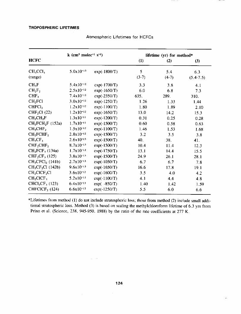
The atmospheric lifetime of HCFCs is determined predominantly by reaction with tropospheric OH.

Stratospheric loss is secondary and may contribute at most 10% of the total budget.

The lifetimes of HCFCs are determined here by three separate approaches:

(1) 2-D chemical transport model with semi-empirical fit to _4CO:

(2) photochemical calculation of 3-D OH fields and integrated loss;

(3) scaling of the inferred CH3 CC13 lifetime by rate coefficients.

Resulting lifetimes from all three independent approaches generally agree within 15%, as shown in the

table below. The integrated losses calculated from the global OH fields in the models (1 & 2) are con-

strained by modelling of the observations and budgets for taco and CH3CDCI3 (respectively). Method

(3) may be expressed simply as

lifetime (HCFC) = 6.3 yr x k(CH3 CCI3 at 277 K) / k(HCFC at 277 K),

where the current estimate of the lifetime for methyl chloroform (6.3 yr) is based on the ALE/GAGE

analysis (Prinn et al., 1987). Some of the errors associated with this scaling have been tested with the

3-D OH fields from method (2); method (3) should be reliable for calculating HCFC lifetimes in the range

1 to 30 years.

The calculated local concentrations of OH in these models (1 & 2) are not well tested since there are few

observations of OH with which to compare. Based on method (2), the middle tropical troposphere (2-6

km) dominates the atmospheric loss and would be an important region in which to make observations of OH.

Estimated uncertainties in the HCFC lifetimes between 1 and 30 years are +50% for (1) and +40%

for (2) & (3). Global OH values that give lifetimes outside of these ranges of uncertainty are inconsistent

with detailed analyses of the observed distributions for 14CO and CH3CCI3. The expected spatial and seasonal

variations in the global distribution of HCFCs with lifetimes of 1 to 30 yr have been examined with methods

(1) & (2) and found to have insignificant effect on the calculated lifetimes. Larger uncertainties apply

to gases with lifetimes shorter than one year; however, for these species our concern is for destruction

on a regional scale rather than global accumulation.

Future changes in the oxidative capacity of the troposphere, due to changing atmospheric composition,

will affect HCFC lifetimes and introduce additional uncertainties of order + 20%.

123

PRECEDING P,_GE BL,':',.f'.JKNOT FILMED

TROPOSPHERICLIFETIMES

Atmospheric Lifetimes for HCFCs

k (cm 3 molec "I s-_) lifetime (yr) for method*

HCFC (I) (2) (3)

CH3CCI3 5.0x10 -t3 exp(- 1800/T) 5 5.4 6.3

(range) (3-7) (4-7) (5.4-7.5)

CH3F 5.4x10 -tz exp(-1700/T) 3.3 3.8 4.1

CH2F2 2.5x10 -lz exp(-1650/T) 6.0 6.8 7.3

CHF3 7.4x10 -13 exp(-2350/T) 635. 289. 310.

CH2FCI 3.0x 10-12 exp(- 1250/T) 1.26 1.33 1.44

CHFClz 1.2x10 -12 exp(- 1100/T) 1.80 1.89 2.10

CHFzCI (22) 1.2x10 -12 exp(-1650/T) 13.0 14.2 15.3

CH3CHzF 1.3x10 -II exp(- 1200/T) 0.31 0.25 0.28

CHzFCHzF (152a) 1.Tx10 -_1 exp(- 1500/T) 0.60 0.58 0.63

CH3CHF2 1.5x 10-'2 exp(- 1100/T) 1.46 1.53 1.68

CHzFCHF2 2.8x10 -12 exp(- 1500/T) 3.2 3.5 3.8

CH3CF3 2.6x10 -'3 exp(- 1500/T) 40. 38. 41.

CHFzCHF: 8.7x 10-13 exp(- 1500/T) 10.4 11.4 12.3

CH2FCF3 (134a) 1.7x10 -t2 exp(-1750/T) 13.1 14.4 15.5

CHF2CF3 (125) 3.8x10 -13 exp(-1500/T) 24.9 26.1 28.1

CH3CFClz (141b) 2.7x10 -t3 exp(- 1050/T) 6.7 6.7 7.8

CH3CF2CI (142b) 9.6x10 -L3 exp(-1650/T) 16.6 17.8 19.1

CH2CICF2C1 3.6x10 -_z exp(- 1600/T) 3.5 4.0 4.2

CH2CICF3 5.2x10 -13 exp(- 1100/T) 4.1 4.4 4.8

CHCI2CF3 (123) 6.4x10 -13 exp(-850/T) 1.40 1.42 1.59

CHFCICF3 (124) 6.6x10 -13 exp(-1250/T) 5.5 6.0 6.6

*Lifetimes from method (1) do not include stratospheric loss; those from method (2) include small addi-

tional stratospheric loss. Method (3) is based on scaling the methylchloroform lifetime of 6.3 yrs from

Prinn et al. (Science, 238, 945-950, 1988) by the ratio of the rate coefficients at 277 K.

124

N92-15439

THE TROPOSPHERIC LIFETIMES OF HALOCARBONS AND THEIRREACTIONS WITH OH RADICALS:

AN ASSESSMENT BASED ON THE CONCENTRATION OF 14CO

Richard G. DerwentModelling and Assessments Group

Environmental and Medical Sciences DivisionHarwell Laboratory

OxfordshireUnited Kingdom

Andreas Volz-ThomasInstitut f_ir Chemie der Belasteten Atmosphere, ICH2

PO Box 1913D5170 Julich

Federal Republic of Germany

PRECEDING PAGE BLAPJK NOT FILMED


EXECUTIVE SUMMARY

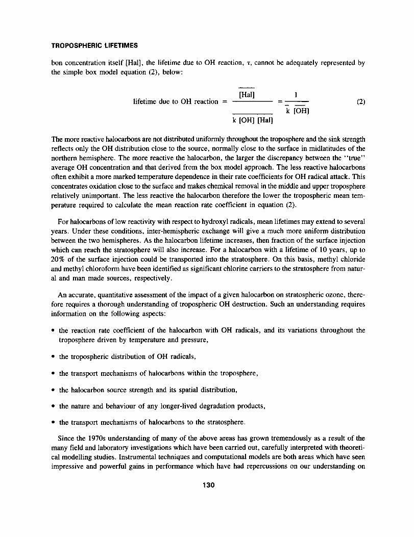
Chemical reaction with hydroxyl radicals formed in the troposphere from ozone photolysis in the presence

of methane, carbon monoxide and nitrogen oxides provides an important removal mechanism for halocar-

bons containing C-H and C = C double bonds. The isotopic distribution in atmospheric carbon monoxide

has been used to quantify the tropospheric hydroxyl radical distribution. This review reevaluates this

methodology in the light of recent chemical kinetic data evaluations and new understanding gained in

the life cycles of methane and carbon monoxide. None of these changes has forced a significant revision

of the _4CO approach. However, it is now somewhat more clearly apparent how important basic chemi-

cal kinetic data are to the accurate establishment of the tropospheric hydroxyl radical distribution.

The two-dimensional (altitude-latitude) time-dependent (seasonal) hydroxyl radical distribution obtained

by the _4CO approach has then been used in the Harwell model to estimate halocarbon lifetimes together

with their confidence limits. A simple graphical procedure suffices to relate halocarbon lifetime to the

pre-exponential factors and activation energy parameters which describe the temperature dependent OH+ halocarbon rate coefficients. Lifetimes and their 1-sigma confidence limits are calculated using the

Harwell two-dimensional model for a range of alternative fluorocarbons.

127

PRECEDING PAGE BLP.r'jK NOT FILMED


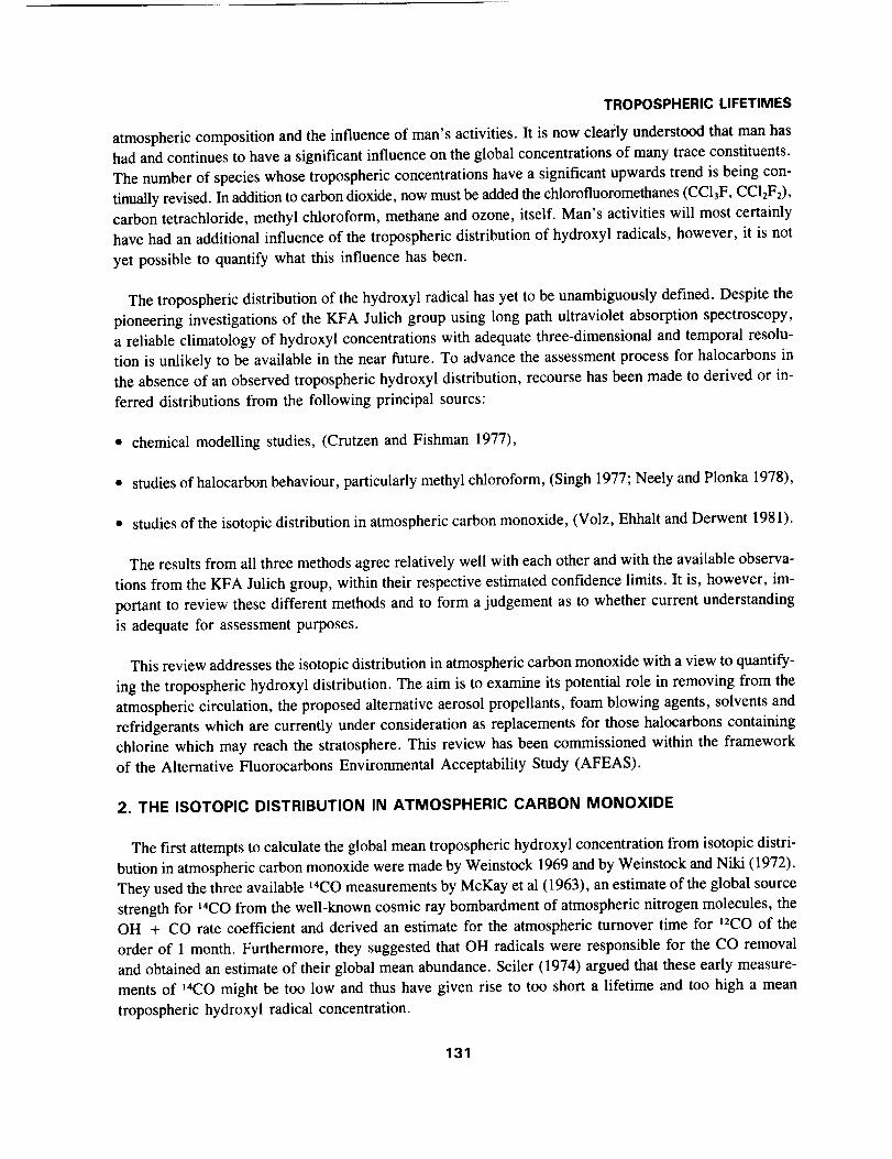
1. INTRODUCTION

The role of homogeneous gas phase reaction in the lower atmosphere was first investigated in the 1950's,

in attempts to understand the phenomenon of photochemical smog and the chemistry involved in its for-

mation (Leighton, 1961). It was Levy (1971) who first suggested that free-radical chemistry, driven by

photochemical dissociation of ozone and nitrogen oxides, might be important in the background troposphere.

He proposed that relatively high concentrations of the reactive hydroxyl radicals could be maintained

in steady state in the background sunlit troposphere and that this steady state could provide an efficient

scavenging mechanism for both natural and man-made trace constituents on a global scale.

Since then attempts have been made to unravel the free-radical chemistry of the troposphere and to quantify

its role in the trace gas cycles. The reactions of the hydroxyl radical in the troposphere have been linked

to a growing list of trace gases including ozone and NO (Levy 1971; Crutzen 1974), carbon monoxide

(Weinstock and Niki 1972), methane (Ehhalt 1974), hydrogen (Seiler and Schmidt 1974) followed somewhat

later by the sulphur compounds (Crutzen 1976) and halocarbons (Cox et al 1976). This review concerns

the distributions of tropospheric hydroxyl radicals and their role in determining the lifetimes of halocar-

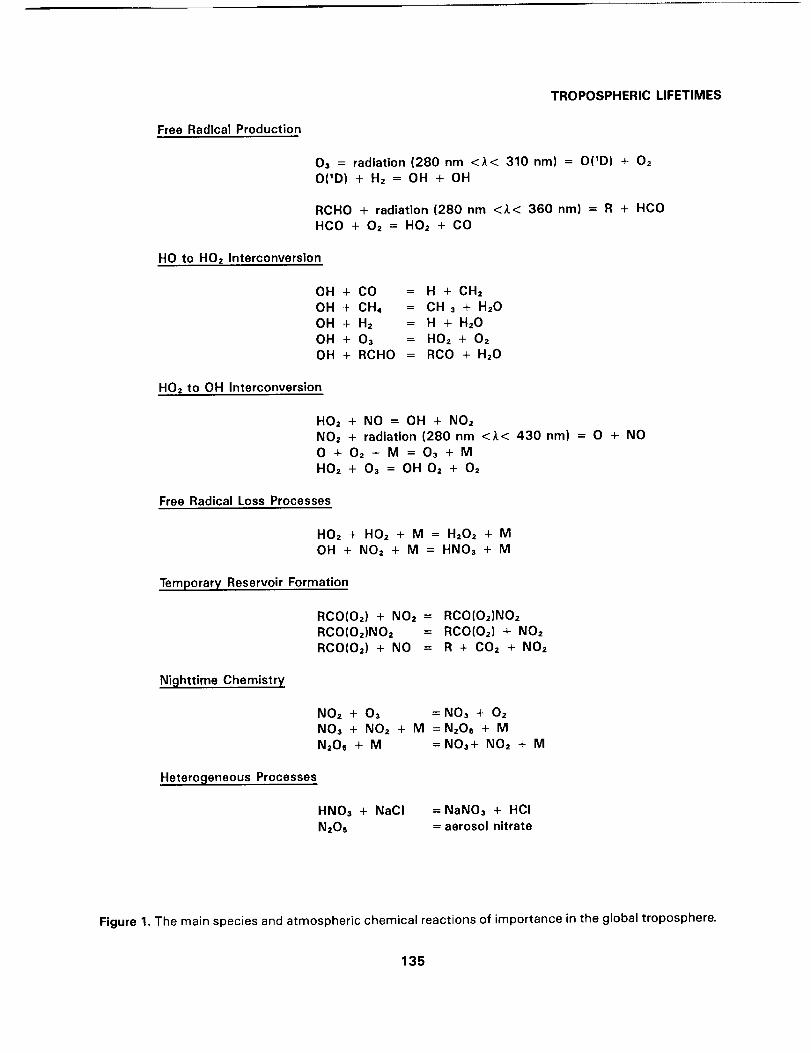
bons. Figure 1 shows some of the species and some of the atmospheric chemical reactions of importance

in the global troposphere.

Interest in tropospheric chemistry has been stimulated by the problem of depletion of stratospheric ozone

by chlorofluoromethanes and other chlorine-containing species (HMSO 1976; NAS 1977). The extent

to which chlorine compounds injected at the earth's surface reach the stratosphere depends on the effi-

ciency with which they are scavenged in the troposphere. Quantitative determination of the sink strength

is required to assess the impact of various chlorine-containing species, both natural and man-made, on

stratospheric ozone.

The scavenging processes acting in the troposphere may be divided into physical removal processes,

in which species are absorbed irreversibly at the earth's surface or in precipitation elements (cloud and

rain droplets, aerosols) and chemical removal processes which involve reactions in the atmosphere. Physical

removal is often referred to as wet and dry deposition and may be highly efficient for some trace consti-

tuents such as ozone, sulphur dioxide and nitric acid. However for halocarbons it is not generally a par-

ticularly efficient process and it may be neglected for most species.

Chemical removal of halocarbons by destruction with tropospheric hydroxyl radicals has been shown

to be an important sink for those halocarbons which contain H atoms and C = C double bonds, (Cox

et al 1976). This sink process may be represented simply by the equation (1), below:

k

OH + Halocarbon _ sink (1)

where k is some temperature dependent OH rate coefficient and OH is some form of globally averaged

concentration of hydroxyl radicals.

Early two-dimensional model studies (Derwent and Eggleton 1978) have shown that because of the covar-

iance of the temperature dependent value of k, the hydroxyl radical concentration [OH] and the halocar-

129

PRECEDING PAG_ i_t.RF_KNOT F;I.r.,,'rE_


bon concentration itself [Hall, the lifetime due to OH reaction, T, cannot be adequately represented by

the simple box model equation (2), below:

lifetime due to OH reaction =[Hall

k [OH] [Hal]

1

k [OH]

(2)

The more reactive halocarbons are not distributed uniformly throughout the troposphere and the sink strength

reflects only the OH distribution close to the source, normally close to the surface in midlatitudes of the

northern hemisphere. The more reactive the halocarbon, the larger the discrepancy between the "true"

average OH concentration and that derived from the box model approach. The less reactive halocarbons

often exhibit a more marked temperature dependence in their rate coefficients for OH radical attack. This

concentrates oxidation close to the surface and makes chemical removal in the middle and upper troposphere

relatively unimportant. The less reactive the halocarbon therefore the lower the tropospheric mean tem-

perature required to calculate the mean reaction rate coefficient in equation (2).

For halocarbons of low reactivity with respect to hydroxyl radicals, mean lifetimes may extend to several

years. Under these conditions, inter-hemispheric exchange will give a much more uniform distribution

between the two hemispheres. As the halocarbon lifetime increases, then fraction of the surface injection

which can reach the stratosphere will also increase. For a halocarbon with a lifetime of 10 years, up to

20% of the surface injection could be transported into the stratosphere. On this basis, methyl chloride

and methyl chloroform have been identified as significant chlorine carriers to the stratosphere from natur-

al and man made sources, respectively.

An accurate, quantitative assessment of the impact of a given halocarbon on stratospheric ozone, there-

fore requires a thorough understanding of tropospheric OH destruction. Such an understanding requires

information on the following aspects:

• the reaction rate coefficient of the halocarbon with OH radicals, and its variations throughout the

troposphere driven by temperature and pressure,

• the tropospheric distribution of OH radicals,

• the transport mechanisms of halocarbons within the troposphere,

• the halocarbon source strength and its spatial distribution,

• the nature and behaviour of any longer-lived degradation products,

• the transport mechanisms of halocarbons to the stratosphere.

Since the 1970s understanding of many of the above areas has grown tremendously as a result of the

many field and laboratory investigations which have been carried out, carefully interpreted with theoreti-

cal modelling studies. Instrumental techniques and computational models are both areas which have seen

impressive and powerful gains in performance which have had repercussions on our understanding on

130


atmospheric composition and the influence of man's activities. It is now clearly understood that man has

had and continues to have a significant influence on the global concentrations of many trace constituents.

The number of species whose tropospheric concentrations have a significant upwards trend is being con-

tinually revised. In addition to carbon dioxide, now must be added the chlorofluoromethanes (CC13F, CC12F2),

carbon tetrachloride, methyl chloroform, methane and ozone, itself. Man's activities will most certainly

have had an additional influence of the tropospheric distribution of hydroxyl radicals, however, it is not

yet possible to quantify what this influence has been.

The tropospheric distribution of the hydroxyl radical has yet to be unambiguously defined. Despite the

pioneering investigations of the KFA Julich group using long path ultraviolet absorption spectroscopy,

a reliable climatology of hydroxyl concentrations with adequate three-dimensional and temporal resolu-

tion is unlikely to be available in the near future. To advance the assessment process for halocarbons in

the absence of an observed tropospheric hydroxyl distribution, recourse has been made to derived or in-

ferred distributions from the following principal sourcs:

• chemical modelling studies, (Crutzen and Fishman 1977),

• studies of halocarbon behaviour, particularly methyl chloroform, (Singh 1977; Neely and Plonka 1978),

• studies of the isotopic distribution in atmospheric carbon monoxide, (Volz, Ehhalt and Derwent 1981).

The results from all three methods agree relatively well with each other and with the available observa-

tions from the KFA Julich group, within their respective estimated confidence limits. It is, however, im-

portant to review these different methods and to form a judgement as to whether current understanding

is adequate for assessment purposes.

This review addresses the isotopic distribution in atmospheric carbon monoxide with a view to quantify-

ing the tropospheric hydroxyl distribution. The aim is to examine its potential role in removing from the

atmospheric circulation, the proposed alternative aerosol propellants, foam blowing agents, solvents and

refridgerants which are currently under consideration as replacements for those halocarbons containing

chlorine which may reach the stratosphere. This review has been commissioned within the framework

of the Alternative Fluorocarbons Environmental Acceptability Study (AFEAS).

2. THE ISOTOPIC DISTRIBUTION IN ATMOSPHERIC CARBON MONOXIDE

The first attempts to calculate the global mean tropospheric hydroxyl concentration from isotopic distri-

bution in atmospheric carbon monoxide were made by Weinstock 1969 and by Weinstock and Niki (1972).

They used the three available _4CO measurements by McKay et al (1963), an estimate of the global source

strength for _4CO from the well-known cosmic ray bombardment of atmospheric nitrogen molecules, the

OH + CO rate coefficient and derived an estimate for the atmospheric turnover time for _2CO of the

order of 1 month. Furthermore, they suggested that OH radicals were responsible for the CO removal

and obtained an estimate of their global mean abundance. Seiler (1974) argued that these early measure-

ments of _4CO might be too low and thus have given rise to too short a lifetime and too high a mean

tropospheric hydroxyl radical concentration.

131


Volz, Ehhalt and Derwent (1981) repeated the methodology and obtained a mean tropospheric hydroxyl

radical concentration of (6.5 ÷ 3 )-2 x 105 molecule cm -3 based on four refinements, viz:

, additional measurements of '4CO in the lower troposphere,

• evaluated chemical kinetic data for the OH + CO reaction,

• improved life cycle data for '4C and '2C in the troposphere,

• a global two-dimensional time-dependent model to investigate the coupled CH4-H2-CO-NOx-O3 life cy-

cles, replacing the box model approach.

In the intervening years since the publication of these early studies (Weinstock and Niki 1972; Volz,

Ehhalt and Derwent 1981), understanding of the oxidizing capacity of the troposphere has developed sig-

nificantly. The paragraphs which follow have therefore been devoted to a reevaluation of some of the

measurements, data and assumptions which were essential in the Volz, Ehhalt and Derwent (1981) study.

The general impression gained from this reevaluation is that subsequent research does appear to have neither

undermined nor found the _4CO method seriously flawed. It therefore remains a viable method for deter-

mining the tropospheric hydroxyl distribution. Nevertheless, some of the input assumptions could now

be questioned in detail and these areas are highlighted and their impact on the determination of the tropospheric

hydroxyl distribution assessed.

The Methodology Used

The methodology adopted by Volz, Ehhalt and Derwent (1981) was to take a precalculated two-dimensional

(altitude, latitude), time-dependent (monthly) field of tropospheric hydroxyl radicals and linearly scale

it until it generated surface '4CO and '2CO concentrations which balanced observations. At the point of

balance, the methodology simultaneously determined the tropospheric hydroxyl distribution and the bio-

genic source strength of _2CO, both of which are coupled unknowns.

The estimated tropospheric hydroxyl distribution contains uncertainties which derive directly from the

uncertain '4CO measurements, the uncertainties in the 14CO and '2CO life cycles, the uncertainties in the

parameters used in the two-dimensional model and the uncertainties inherent all the assumptions made

in the model formulation itself. The uncertainty analysis treatment in Volz, Ehhalt and Derwent (1981)

considered the contributions from the likely errors in:

• the '4CO production from cosmic rays, (Lingenfelter 1963),

• the '_CO emission from fossil fuel burning, (Seiler 1974; Logan et al 1981),

• the _4CO measurements, (McKay et al 1963; Volz, Ehhalt and Derwent 1981),

• the '2CO latitudinal distribution, (Seiler and Schmidt 1974),

• the transport and chemistry schemes employed in the two-dimensional model, (Derwent and Curtis 1977).

132


Experimental Techniques

The measurement of the concentration of _4CO is essential to the 14CO approach. The early measure-

ments of McKay et al 1963 relied on the isotopic ratio viz. 14CO/12CO in air samples obtained from

an air liquefaction plant. McKay et al however failed to determine simultaneously the _2CO concentra-

tion and this led to the introduction of uncertainties in using the _4CO approach. A major challenge

in the study by Volz, Ehhalt, Derwent and Khedim (1979) was therefore the measurement of the t4COconcentration.

Volz, Ehhalt, Derwent and Khedim (1979) have described their experimental procedures in some

detail and only a brief outline is given in the paragraphs below. The procedure consists of two steps,

• the quantitative separation and the collection of the CO from ambient air,

• the determination of its isotopic ratios, Rco = [14CO]/[12CO].

The _4CO concentration is then given by:

[14CO ] = Roo. [12CO]

The separation of the CO from ambient air was achieved by quantitative oxidation to COz on a hot plati-

num catalyst, followed by absorption in CO2-free aqueous NaOH. Prior to this the atmospheric CO2 was

removed from the air sample by absorption in NaOH. Interferences from any remaining CO2 were deter-

mined by gas chromatography and were found to be less than 5 %. The CO concentration in the air was

measured by gas chromatography and, in addition, calculated from the amount of CO collected and the

volume of air sampled, (100-200 m3).

The isotopic ratio of the sampled CO was measured in a low-level counting system, similar to those

used for t4C dating, with an accuracy of + 3-5 %. The counting system was calibrated against the t4CO

standard of the Institut fiir Umweltphysik, Universitat Heidelberg. The overall accuracy in the determina-

tion of the _4CO concentration was largely determined by uncertainties associated with the sampling procedure

as discussed by Volz, Ehhalt, Derwent and Khedim (1979), and was generally on the order of + 10%

(lo), including any possible systematic bias.

Measured _4CO Concentrations

So far measurements of the _4CO concentration have been reported only for the northern hemisphere,

(Volz, Ehhalt and Derwent 1981). Most of the samples were collected during 1977 and 1978 at a remote,

rural site in the Eifel mountains (51°N 2°W) in the Federal Republic of Germany. In addition, three sam-

ples were collected during a cruise of the RV Knorr over the Mediterranean Sea and the Atlantic (36 o

to 46°N) in April 1976 and two samples at Miami, Florida (27°N) in September 1977, (Volz, Ehhalt,

Derwent and Khedim 1979).

The t4CO concentration data exhibit a well-defined seasonal cycle with a winter maximum of about

20 molecule cm -3 and a summer minimum of 10 molecule cm -3. The annual cycle in ]4CO reflects the

influence of the chemical sink due to destruction by tropospheric OH radicals.

133


The laCO concentration data also show evidence of a latitudinal gradient increasing from the equator

to the North Pole. The concentrations at Miami (27°N) in September 1972, 4.2 + 0.7 molecule cm -3

are almost a factor of three smaller than those found at 51°N for the same time of year. Similarly, the

concentrations measured over the Atlantic Ocean show an increase from 15 molecule cm- 3 at 36°N to

19 molecule cm -3 at 43°N. This latitudinal distribution in 14CO reflects the influence of the tropospheric

OH distribution increasing from the North Pole towards the equator.

Evaluated Rate Coefficient Data

An important aspect of the two-dimensional model used to calculate the tropospheric distribution of

hydroxyl radicals, is the chemical kinetic input data adopted. Figure 1 illustrates the main free radical

reactions which are believed to be occurring in the sunlit free troposphere. To a degree, the OH distribu-

tion estimated by Volz, Ehhalt and Derwent (1981) is sensitive to all the chemical kinetic assumptions.

However, some of the chemical kinetic input parameters exert a more significant influence on the OH

concentrations than others and it is upon these that we have concentrated upon in the paragraphs below.

The Volz, Ehhalt and Derwent (1981) paper drew much of its chemical kinetic input data from the 1979

CODATA review (Baulch et al 1980). This can be directly compared with the 1988 IUPAC evaluation

(Atkinson et al 1989).

OH to HO2 interconversion reactions

The conversion of hydroxyl to hydroperoxyl radicals is driven largely by the reaction of OH radicals

with carbon monoxide, methane and hydrogen. There has been an important revision in the OH + CO

rate coefficient over the intervening years from 1.4 x 10-_3 (1 + Patm) cm3 m°lecule-I s-_ to 1.5 x 10"t3

(1 + 0.6 Patm) cm3 m°lecule-I s-t" This reevaluation reduces the rate coefficient by 14% at 1 atmosphere

pressure and increases it by about 3 % under the conditions in the upper troposphere. There have beenrevisions to the OH + CH4 and OH + H2 rate coefficients. Under the conditions approproate to the lower

troposphere, the OH + CH4 rate coefficient has been increased by about 6%, whereas the OH + H2

rate coefficient has decreased by about 4 %. Overall, these latter reevaluations are not likely to be signifi-

cant compared with that of the OH + CO reaction.

In the two-dimensional model study, the concentration fields of CO, CH4 and H2 were taken from the

available measurements and sufficient CO, CH4 and H2 were injected into the model at every time step

to balance removal by all processes in the surface layer including the reaction with hydroxyl radicals.

If a lower OH + CO rate coefficient had been employed then, to maintain the same OH --* HO2 flux,

a 10-15% higher OH concentration would be required.

HO2 to OH interconversion reactions

The conversion of HO2 radicals to OH radicals is largely driven by the reactions of HO2 radicals with

ozone and nitric oxide. The rate coefficients of these two reactions under conditions appropriate to lower

troposphere have not changed by more than 1-7 %. These reevaluations are of negligible importance.

HO2 recombination to form hydrogen peroxide

The recombination of HO2 radicals to form hydrogen peroxide dominates free radical termination in

the free troposphere at all heights and latitudes where NOx levels are low. The reaction has generally

134


Free Radical Production

03 = radiation (280 nm <Z< 310 nm) = O(1D) + Oz

O(ID) + H2 = OH + OH

RCHO + radiation (280 nm <Z< 360 nm) = R + HCO

HCO + O= = HOz + CO

HO to HO= Interconversion

OH + CO = H + CH=

OH + CH, = CH 3 + H20

OH + H= = H + H=O

OH + 03 = HO= + O=OH + RCHO = RCO + HzO

HO= to OH Interconversion

HO= + NO = OH + NOz

NO2 + radiation (280 nm <_< 430 nm) = 0 + NO

0 + 02 + M = 03 + M

HO= + 02 = OH 02 + 02

Free Radical Loss Processes

HO= + HO= + M = H20= + MOH + NO= + M = HN03 + M

Temporary Reservoir Formation

RCO(O=) + NO2 =RCO(Oz)NOz =

RCO(O=) + NO =

RCO(O2)NOz

RCO(Oz) + NO=R + COz + NOz

Nighttime Chemistry

NO2 + 03 =NO3 + O=

NO3 + NOz + M =N=Os + M

Nz06 + M = NO3+ NOz + M

Heterogeneous Processes

HN03 + NaCI

NzOs

= NAN03 + HCI

= aerosol nitrate

Figure 1. The main species and atmospheric chemical reactions of importance in the global troposphere.

135


not been intensively investigated in laboratory chemistry studies and evaluations have had only a few studies

to draw upon. It is not surprising to find that this reaction has undergone a dramatic reevaluation between

the 1979 CODATA (Baulch et al 1980) and 1988 IUPAC (Atkinson et al 1989) studies. The unusually

large negative activation energy reported previously has been replaced by a significantly smaller but neverthe-

less still negative value. The effect of the reevaluations is to produce a HO2 + HO2 rate coefficient which

is about a factor of 1.7 lower in the lower troposphere and a factor of 4 lower in the upper troposphere.

Because of the square dependence of the free radical destruction rate on the HO2 radical concentration,

the reevaluation of the HO2 + HO2 rate data should lead to OH and HO2 radical concentrations about

a factor of two higher in the upper troposphere and about thirty percent higher in the lower troposphere.

The reevaluations in the chemical kinetic data indeed strengthen the results of Volz, Ehhalt and Der-

went, 1981: at the time of their evaluation, the OH concentrations required to balance the budgets of both

'2CO and '4CO were a factor of 1.7 greater than those derived from photochemical models. It appears

now that inadequacies in the chemical kinetic data, most important the rate coefficients for the OH +

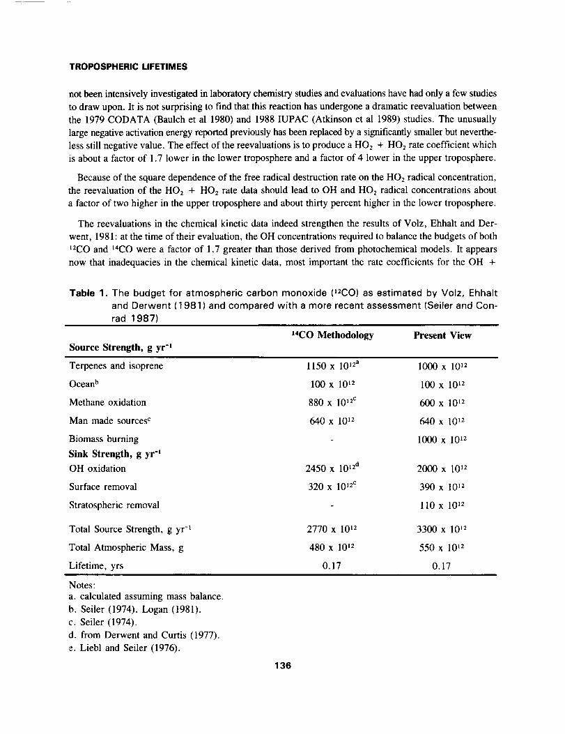
Table 1. The budget for atmospheric carbon monoxide (12CO) as estimated by Volz, Ehhaltand Derwent (1981) and compared with a more recent assessment (Seiler and Con-

rad 1987)

Source Strength, g yr "1

t4CO Methodology Present View

Terpenes and isoprene

Ocean b

Methane oxidation

Man made sources c

Biomass burning

Sink Strength, g yr "1

OH oxidation

Surface removal

Stratospheric removal

Total Source Strength, g yr -1

Total Atmospheric Mass, g

Lifetime, yrs

1150 x 1012a 1000 x 1012

100 x 1012 100 x 1012

880 x 1012c 600 x 1012

640 x 1012 640 x 1012

1000 x 1012

2450 x 1012d 2000 x 1012

320 x 1012e 390 x 1012

110 x 1012

2770 x 1012 3300 x 1012

480 x 1012 550 x 1012

0.17 0.17

Notes:

a. calculated assuming mass balance.

b. Seiler (1974). Logan (1981).

c. Seiler (1974).

d. from Derwent and Curtis (1977).

e. Liebl and Seiler (1976).

136


CO and HO2 + HO2 reactions, indeed resulted in too low OH concentrations in the photochemical models

at that time. With the revised rate coefficients, the OH distributions from _4CO and from photochemical

models are in much better agreement.

Life Cycle Data

Inherent in the methodology were some basic assumptions concerning the methane, carbon monoxide,

hydrogen, nitrogen oxides and ozone life cycles in the two-dimensional model of t4CO and in the two-

dimensional model used to estimate the hydroxyl radical concentrations, themselves. At the point where

the _2CO and _4CO distributions balanced, the methodology returned the biospheric source strength of

_2CO allowing a solution to the tECO budget.

In Table l, this budget is examined in some detail and compared with a more recent evaluation by Seiler

and Conrad (1987). The overall conclusion is that the broad features of the carbon monoxide budget have

remained unchanged. In detail, though, there is a major difference in the significance given to biomass

burning. The Volz, Ehhalt and Derwent (1981) study was unable to resolve the difference between bi-

omass burning, on the one hand, and terpene and isoprene oxidation on the other, as both are sources

of t4CO and t2CO. Subsequently, field campaigns in the tropical regions of South America have led to

a quantification of this source as shown in Table 1.

The inclusion of the biomass burning source would have an impact on the Volz, Ehhalt and Derwent

(1981) analysis because of the different latitudinal distributions of the t2CO and 14CO source strengths.

Adrigole 52°N210

205

Q.

uc 200

ot_

195

190

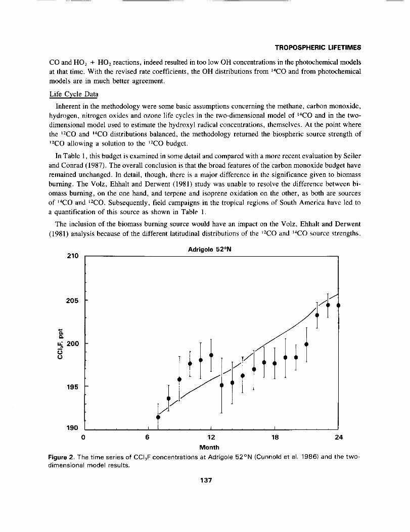
Figure 2. The time series of CCI3F concentrations at Adrigole 52°N (Cunnold et al. 1986) and the two-dimensional model results.

137


205

200

K

195¢J¢J

190

Cape Meares 45°N

t

185 ..... t ..... t ..... J

0 6 12 18 24Month

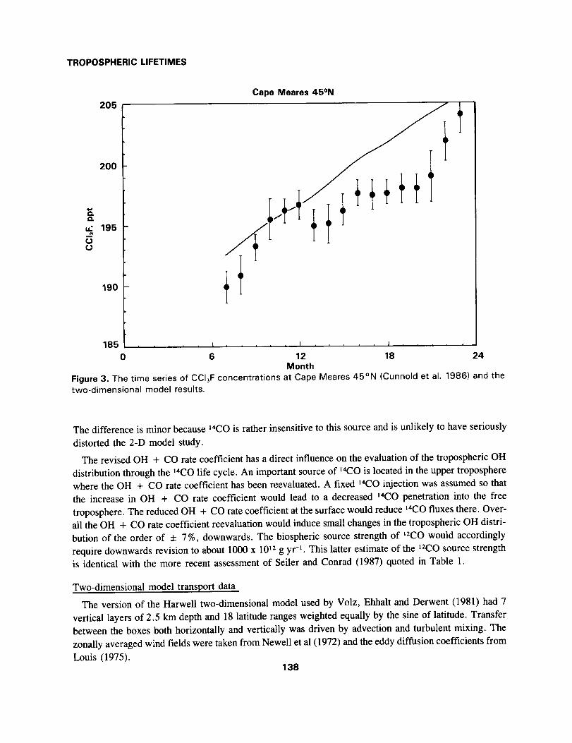
Figure 3. The time series of CCI3F concentrations at Cape Meares 45°N (Cunnold et al. 1986) and thetwo-dimensional model results.

The difference is minor because 14CO is rather insensitive to this source and is unlikely to have seriously

distorted the 2-D model study.

The revised OH + CO rate coefficient has a direct influence on the evaluation of the tropospheric OH

distribution through the 14CO life cycle. An important source of 14CO is located in the upper troposphere

where the OH + CO rate coefficient has been reevaluated. A fixed t4CO injection was assumed so that

the increase in OH + CO rate coefficient would lead to a decreased _4CO penetration into the free

troposphere. The reduced OH + CO rate coefficient at the surface would reduce _4CO fluxes there. Over-

all the OH + CO rate coefficient reevaluation would induce small changes in the tropospheric OH distri-

bution of the order of :t: 7%, downwards. The biospheric source strength of _2CO would accordingly

require downwards revision to about 1000 x 1012 g yr -1. This latter estimate of the t2CO source strength

is identical with the more recent assessment of Seiler and Conrad (1987) quoted in Table 1.

Two-dimensional model transport data

The version of the Harwell two-dimensional model used by Volz, Ehhalt and Derwent (1981) had 7

vertical layers of 2.5 km depth and 18 latitude ranges weighted equally by the sine of latitude. Transfer

between the boxes both horizontally and vertically was driven by advection and turbulent mixing. The

zonally averaged wind fields were taken from Newell et al (1972) and the eddy diffusion coefficients from

Louis (1975).138


205

200

KQ.

1950

190

185

Ragged Point 13°N

I

0

4I

6 12 18 24Month

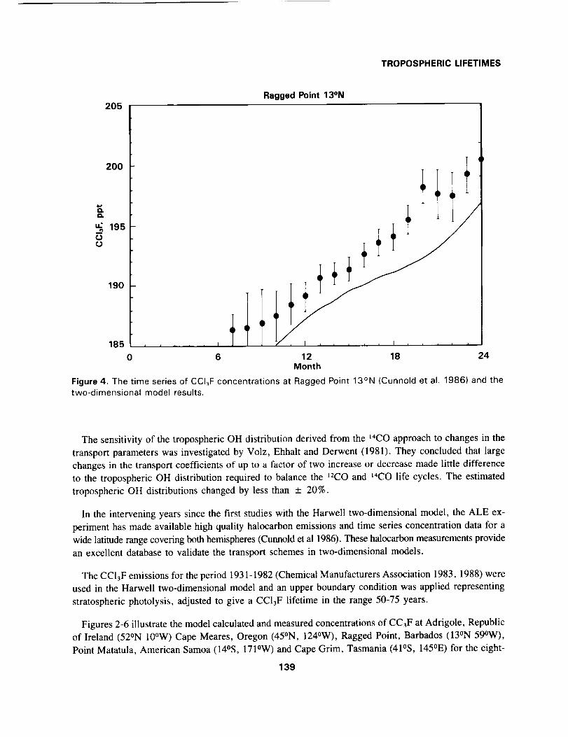
Figure 4. The time series of CCI3F concentrations at Ragged Point 13°N (Cunnold et al. 1986) and thetwo-dimensional model results.

The sensitivity of the tropospheric OH distribution derived from the t4CO approach to changes in the

transport parameters was investigated by Volz, Ehhalt and Derwent (1981). They concluded that large

changes in the transport coefficients of up to a factor of two increase or decrease made little difference

to the tropospheric OH distribution required to balance the 12CO and t4CO life cycles. The estimated

tropospheric OH distributions changed by less than _+ 20%.

In the intervening years since the first studies with the Harwell two-dimensional model, the ALE ex-

periment has made available high quality halocarbon emissions and time series concentration data for a

wide latitude range covering both hemispheres (Cunnold et al 1986). These halocarbon measurements provide

an excellent database to validate the transport schemes in two-dimensional models.

The CC13F emissions for the period 1931-1982 (Chemical Manufacturers Association 1983, 1988) were

used in the Harwell two-dimensional model and an upper boundary condition was applied representing

stratospheric photolysis, adjusted to give a CC13F lifetime in the range 50-75 years.

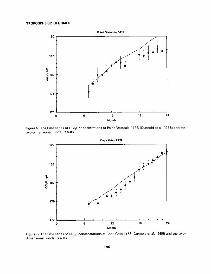
Figures 2-6 illustrate the model calculated and measured concentrations of CC_F at Adrigole, Republic

of Ireland (52°N 10°W) Cape Meares, Oregon (45°N, 124°W), Ragged Point, Barbados (13°N 59°W),

Point Matatula, American Samoa (14°S, 171°W) and Cape Grim, Tasmania (41°S, 145°E) for the eight-

139


190

185

D.

180(J¢J

175

170

Point Matatula 14°S

I I

0 6 12 18 24

Month

Figure 5. The time series of CCI3F concentrations at Point Matatula 14°S (Cunnold et al. 1986) and thetwo-dimensional model results.

Cape Grim 41°S

190

185

O.

_80

0

175

+Y

170 , , , I ..... I I .....

0 6 12 18 24

Month

Figure 6. The time series of CCI3F concentrations at Cape Grim 41°S (Cunnold et al. 1986) and the two-

dimensional model results.

140


een month period from July 1981 to December 1982 (Cunnold et al 1986). Viewed against the ALE meas-

urements, the transport scheme in the Harwell two-dimensional model is clearly performing adequately

and without systematic bias.

The conclusion is that the transport scheme adopted in the Volz, Ehhalt and Derwent (1981) study represents

adequately the gross features of halocarbon transport and this is an important model validation. Further-

more, the sensitivity of the estimated tropospheric OH distribution to the magnitudes of the transport coeffi-

cients is not strong. It is unlikely therefore that inadequacies in present understanding of global transport

have seriously influenced the uncertainty in the estimated tropospheric OH distribution using the '4CO method.

3. THE TROPOSPHERIC DISTRIBUTION OF OH RADICALS AND HALOCARBON LIFETIMES

Halocarbon Lifetimes

The behaviour of a halocarbon in a two-dimensional (altitude-latitude) atmosphere injected at the earth's

surface, subject to stratospheric destruction and oxidation by hydroxyl radicals can be described by the

differential equation:

d [Hal] + div ([Hal] . U) - div (K.N. grad ([Hal]/N)

dt

= E - k[OH][Hal] - SL[Hal] (3)

The time behaviour of the halocarbon concentration [Hal] in molecule cm -3 was computed by solving

the above continuity equation over a 6 x 18 mesh point grid extending vertically in 2.5 km steps and in

18 steps latitudinally with equal spacing in sine _ where _ is the latitude angle. The two-dimensional wind

field, U, and the eddy diffusion tensor, K, were taken from Newell et al (1972) and Louis (1975), respec-

tively. The detailed procedures used in the finite-differencing scheme have been described elsewhere (Derwent

and Curtis 1977). The finite difference form of the above equation was integrated numerically using the

Harwell program FACSIMILE (Curtis and Sweetenham 1987). For a 100 year model simulation, 15 minutes

computer time were required using an IBM compatible 80386/80387-based microcomputer (Dell System 310).

The terms in the above continuity equation describing the halocarbon behaviour were derived as follows:

• E: a time-independent halocarbon injection was assumed with a spatial distribution which closely fol-

lowed the population distribution between the hemispheres,

• SL: stratospheric loss coefficient, which was set to give a lifetime due to stratospheric removal, acting

on its own, of 50-100 years,

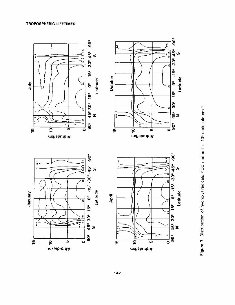
• [OH]: this is the time dependent two-dimensional distribution of tropospheric hydroxyl radicals deter-

mined by Volz, Ehhalt and Derwent (1981) and illustrated in figure 7,

• k: this is the temperature dependent rate coefficient for hydroxyl radical attack on the halocarbon of interest.

141


m

o

U3 0 U3t=-

uJN/epm,!J, IV

0

O_i

o

o

0

i

oUD

,,_1

¢,q

o

_z

o

00'_

Ii.

o ......__..__._.

UD

[I j

-.,,,

0

_._.._...--°_

_o

1,0 0

mN/epm.!_lV

o

o

"o

o

003

o

o

00')

Z

E

0,)

cD

0

E

¢-

0r-

E

O

,d-

03

X

>-c-

O

t-O,,i-a

°_

t_

r,:

0')

I.,I,.

142

>,

E

.J

Q;

dE

.-J


L.)I 'q 'tuJe; fSJeu9 uo!_.ehp,:)V

0 0 0 0 0 0 0 0 0 00 0 0 0 0 0 0 0 0 0

00

0

qr,,

oCD

q

0

otN

0

If)

0

_m

0

ECO

o o

c-

E

m

°--

e- Q

?

e-

Eo

-z_ _/_ E

"_ e- .--

O "-

E EE

'_ mx::

E

i

c-O "t- _

? "_

143


At the end of the 100 year model experiment, the total model halocarbon inventory was divided by the

total halocarbon injection rate to determine the halocarbon lifetime. The assumption of fixed tropospheric

hydroxyl radical concentrations implies low tropospheric halocarbon loadings so as not to perturb the

tropospheric hydroxyl radical concentrations. For reactive halocarbons, this implies that halocarbon con-

centrations are not more than 1 ppb at the most.

Figure 8 shows the total lifetimes including both tropospheric OH oxidation and stratospheric removal

calculated for various assumptions concerning the form of the temperature dependent OH + halocarbon

rate coefficient. Clearly, this temperature dependent parameter exerts a dominant influence on halocarbon

lifetime, with lifetimes covering 0.2 - 30 years for reasonable ranges in expected values of preexponential

factors and activation energies.

However the _4CO method is not uncertainty-free and its accuracy and precision as a means of deter-

mining halocarbon lifetime is dependent on a whole range of experimental, life cycle and modelling as-

sumptions which may be called into question. Volz, Ehhalt and Derwent (1981) gave some thought to

uncertainty limits on their tropospheric OH distribution which this reevaluation has not changed. They

recommended a mean tropospheric OH concentration of 6.5 +_3molecule cm -3. Assuming that the kinet-

ic parameters defining the OH + halocarbon rate coefficient are described with complete certainty, we

can use the 1-sigma confidence limits for the tropospheric OH distribution to determine the confidencelimits of the halocarbon lifetime. The Harwell two-dimensional model was therefore rerun with the entire

tropospheric OH distribution scaled upwards and downwards to the 1-sigma confidence limits. The result-

ing upper and lower 1-sigma confidence limits of the halocarbon lifetimes encompassed the range of a

factor of two for all the halocarbons examined. Lifetimes were apparently slightly more accurately deter-

mined for the longer-lived halocarbons, reflecting the influence of the assumed constant stratospheric removal.

Lifetimes of Alternative Fluorocarbons

For some of the candidate alternative fluorocarbons evaluated chemical kinetic data for the OH + halocar-

bon degradation reactions are already available, Table 2. The lifetimes of these halocarbons due to stratospher-

ic removal and tropospheric OH radical degradation can therefore be determined using the Harwell

two-dimensional model. Table 2 gives the atmospheric lifetimes calculated for a constant injection in mid-

latitudes of the northern hemisphere from a 100 year model calculation. The tropospheric OH distribution

calculated with the _4CO method gives lifetimes for the alternative fluorocarbons in the range 0.3-635

years. For most of the alternative halocarbons, these lifetimes are considerably shorter than the corresponding

lifetimes for the fully halogenated halocarbons.

To complete the environmental acceptability work, modelling studies are required following up the be-

haviour of any chlorine-containing molecular fragments produced by the halocarbon degradation. The be-

haviour of the fragments could readily be incorporated into the two-dimensional model to determine the

magnitude of any stratospheric fluxes of species such as COC12, COHC1, CF3COCI, CFC12CHO,

CFCI2CO(O2)NO2, CF2CICHO, CF2C1CO(O2)NO2, COFC1 and so on. Competing processes for these

chlorine-containing fragments would include tropospheric degradation, dry deposition, photolysis and wet

scavenging.

144


Table 2. OH + halocarbon rate coefficients and atmospheric lifetimes for a range of alternative

fluorocarbons

Formulae

Lifetime, c

OH + halocarbon rate coefficient, yrscm 3 molecule-i s-_ Stratospheric None

loss

CH3F 5.4 x 10-lz exp(-1700/T) 3.12 3.33

CHzFz 2.5 x 10-lz exp(-1650/T) 5.40 6.0

CHF3 7.4 x 10-13 exp(-2350/T) 46.35 635.0

CHzFCI 3.0 x 10-12 exp(-1250/T) 1.23 1.26

CHFC12 1.2 x 10-_2 exp(-I IO0/T) 1.74 .80

CHF2CI 1.2 x 10-12 exp(-1650/T) 10.35 13.0

CH3CH_F 1.3 x 10-11 exp(-1200/T) 0.31 0.31

CHzFCH2F 1.7 x 10-I1 exp(-1500/T) 0.59 0.60

CH3CHF2 1.5 x 10-lz exp(-llOO/T) 1.42 1.46

CH2FCHF2 2.8 x 10 -12 exp(-15OO/T) 2.98 3.17

CH3CF3 2.6 x 10-13 exp(-1500/T) 22.29 40.2

CHFzCHFz 8.7 x 10-13 exp(-1500/T) 8.64 10.4

CHzFCF3 1.7 x 10 -lz exp(-1750/T) 10.40 13.1

CHF2CF3 3.8 x 10 -13 exp(-1500/T) 17.06 25.9

CH3CFCIz 2.7 x 10-13 exp(-1050/T) 5.89 6.68

CH3CFzC1 9.6 x 10-_3 exp(-1650/T) 12.49 16.6

CHzC1CFzC1 3.6 x 10-lz exp(-1600/T) 3.28 3.51

CH2C1CF3 5.2 x 10-13 exp(-1100/T) 3.80 4.11

CHC12CF3 6.4 x 10-13 exp(-850/T) 1.36 1.40

CHFC1CF3 6.6 x 10-13 exp(-1250/T) 4.99 5.54

Notes:

a. Chemical kinetic data from Hampson, Kurylo and Sander (1989)

b. T is absolute temperature in Kc. Lifetimes in steady state have been determined in a two-dimensional model assuming a northern

hemispheric and constant injection rate, allowing for either 2 % yr stratospheric removal or notd. The l-sigma confidence limits on the lifetimes encompass a range of a factor of two.

145


4. CONCLUSIONS

A review of the 14CO method for determining the tropospheric hydroxyl radical distribution has rev-

ealed a number of areas where changes have occurred since the original publication of Volz, Ehhalt and

Derwent (1981). None of these changes has however forced a revision of the approach. They have served

to complete our understanding of areas which were difficult to understand in the early work. The chemical

kinetic data is notable in this regard. It is now much easier to understand why the early hydroxyl radical

concentrations may have been under-estimated in the photochemical models as compared to the 14COevaluation.

For the expected OH + halocarbon chemical rate coefficient parameters defined in terms of preex-

ponential factors and activation energies, it is possible to estimate resulting halocarbon lifetimes using

a simple graphical procedure. The '4CO approach allows the determination of tropospheric halocarbons

lifetimes, halocarbons with reasonable precision, 1-sigma confidence limits spanning about a factor of two.

It is important to remember that OH + halocarbon rate coefficients, hydroxyl distributions and halocar-

bon concentrations exhibit important covariance terms so that halocarbon lifetimes are not well-determined

quantities. The lifetimes determined in this review are valid only for halocarbons injected at the northern

hemisphere surface over the latitude range of the major continental land masses and population centres.

To illustrate the L4CO method, the graphically determined lifetimes for methane and methyl chloroform+3

are found to be 7 -2 and 5 ± 2 years, respectively, which are in close accord with our two-dimensional

model studies (Cox and Derwent 1981; Derwent and Eggleton 1978), and current literature evaluations

(Ehhalt 1988; Prinn 1988). The current methyl chloroform lifetime overlaps the ALE/GAGE evaluation,6.3 + 1.2-0.9 years and confirms both estimates since they are completely independent.

Lifetimes of some candidate alternative fluorocarbons have been tabulated in Table 2 based on detailed

studies using the Harwell two-dimensional model. These studies should be readily extended to include

the subsequent transport and fate of the secondary degradation products liberated by OH attack on the

parent halocarbon.

There is mounting evidence that man's activities are inducing changes in the composition of the global

atmosphere (Rowland and Isaksen 1988). Some of the trace gases for which global trends are beginning

to become characterised play an important role in global tropospheric chemistry, as described in figure

1. In considering the environmental acceptability of alternative fluorocarbons, an attempt should be made

to investigate their tropospheric sinks in future scenarios in which the composition of the global troposphere

has been grossly perturbed by man's activities. For example, future subsonic aircraft operations may in-

crease local tropospheric OH concentrations (Derwent 1982) and other perturbations can be put forward

that would decrease tropospheric OH concentrations. A scenario approach could help to put upper and

lower bounds on the lifetimes of alternative fluorocarbons over the next 50 years.

5. ACKNOWLEDGEMENTS

The two-dimensional modelling work at Harwell employed in this review was sponsored as part of the

United Kingdom Department of the Environment Air Pollution Research Programme.

146

N92-15440

TROPOSPHERIC HYDROXYL CONCENTRATIONS AND THE LIFETIMES OF

HYDROCHLOROFLUOROCARBONS (HCFCs)

Michael J. Prather

NASA/GISS

2880 Broadway, New York, NY 10025

PRECEDING PAGE BLp._;K NGT F;LMED

TROPOSPHERICHYDROXYL

ABSTRACTThree-dimensional fields of modeled tropospheric OH concentrations are used to calculate lifetimes against

destruction by OH for many hydrogenated halocarbons, including the CFC alternatives (hydroch-

lorofluorocarbons or HCFCs). The OH fields are taken from a 3-D chemical transport model (Spivakovsky

et al., 1989) that accurately simulates the global measurements of methyl chloroform (derived lifetime

of 5.5 yr). The lifetimes of various hydro-halocarbons are shown to be insensitive to possible spatial vari-

ations and seasonal cycles. It is possible to scale the HCFC lifetimes to that of methyl chloroform or methane

by using a ratio of the rate coefficients for reaction with OH at an appropriate temperature, about 277 K.

1. INTRODUCTION

Synthetically produced halocarbons that contain chlorine and bromine, often called chlorofluorocarbons

(CFCs) and halons, pose a direct threat to the stratospheric ozone layer (e.g., NASA/WMO, 1986; Wat-

son et al., 1988) and also contribute substantially to the greenhouse forcing of the climate (Ramanathan,

1975; Lacis et al., 1981). A single characteristic of CFCs and hal ons that aggravates these environmental

problems is their long atmospheric lifetimes; most are destroyed only by ultraviolet sunlight in the

stratosphere. As a result of these environmental concerns, there will soon be international restrictions on

CFC growth as agreed upon in the Montreal Protocol, and there is now a search for alternative fluorocar-

bons, environmentally acceptable substitutes (AFEAS Workshop, 16-17 May 1989, Boulder Colorado).

One key property of these alternative compounds must be a short atmospheric residence time, implying

efficient loss in the troposphere or at the Earth's surface.

Many of the suggested alternative fluorocarbons contain hydrogen (hydrochlorofluorocarbons or HCFCs),

and atmospheric loss of these HCFCs is dominated by reaction with tropospheric OH. Their buildup in

the atmosphere (units: kg) will be controlled by the ratio of emissions (kg yr -t) to atmospheric destruction

(yr-t). The globally averaged, annual mean lifetime (yr) of the HCFCs (against atmospheric loss) is de-

fined as the global atmospheric content (kg) divided by the total annual loss (kg yr'l).

In this report we derive the lifetime of HCFCs and other hydrogenated halocarbons in two ways. The

primary method involves modelling the OH distribution from first principles, specifying or predicting the

HCFC distribution, and then integrating the HCFC loss over the globe (e.g., Logan et al., 1981). The

tropospheric OH fields are calculated from a global 3-D climatology of sunlight, temperature, 03, H20,

NOx, CO, CH4 and other hydrocarbons (see Spivakovsky et al., 1989). Uncertainties in the calculated

OH concentrations occur not only with the kinetic model, but also with the global climatologies of the

other trace gases and cloud-cover needed as input to the photochemical model.

The OH fields used here were developed and applied to study methyl chloroform in a 3-D Chemical

Transport Model (CTM). With the CTM, we specified sources, global transport and chemical losses of

CH3CC13 in order to simulate the latitudinal and seasonal patterns, and the global trends (see Spivakovsky

et al., 1989). Similar CTM modelling of all the HCFCs is impractical and would require also a history

and geographical location of emissions. Instead, the four-dimensional OH field (latitude x longitude x

altitude x time) is applied here to test various hypotheses on the sensitivity of HCFC lifetimes to their

tropospheric distribution; it is used also to test the accuracy of scaling the HCFC lifetimes to an assumed

methyl chloroform lifetime.

149

PRECEDING PAGE BLP_,'K NGT F;LMED

TROPOSPHERIC HYDROXYL

The second method for deriving HCFC lifetimes selects a reference species with a global budget and

atmospheric lifetime (against OH destruction) that is thought to be well understood (see Makide and Rowland,

1981). The lifetime of methyl chloroform, CH3CC13, derived from the ALE/GAGE analysis is often used

(Prinn et al., 1987) and is then scaled by the ratio of the rate coefficients for reaction with OH (Hampson,Kurylo and Sander, AFEAS, 1989), k(OH + CH3CC13)/k(OH + HCFC), to calculate the HCFC lifetime.

Possible errors in this approach are associated with the assumed lifetime for CH3CC13, and with the use

of a single scaling factor that does not reflect the different spatial distribution of the HCFCs. This scaling

approximation is tested here for plausible global patterns in the HCFC concentration and for different

temperature dependence of the rate coefficients.

The tropospheric chemistry model for OH is described in Section 2. We calculate the global losses for

methane and methyl chloroform in Section 3, and then compare the results for methyl chloroform with

other published values. The integrated losses for a range of possible distributions of an HCFC are givenin Section 4. HCFC lifetimes and uncertainties are discussed in Section 5.

2. THE CHEMICAL MODEL

The lifetimes calculated here for the HCFCs, as well as for CH3CCI3, CH3CI, CH3Br and CH4, use

global distributions of OH from the photochemical model developed for the 3-D Chemical Transport Model

(CTM developed at GISS & Harvard). The model for tropospheric OH is based on a 1-D photochemical

model (an updated version of Logan et al., 1981 ; DeMore et al., 1987) that has been used to parameterize

OH concentrations as a function of sunlight and other background gases (see Spivakovsky et al., 1989).

This parameterized chemistry has been used to calculate a three-dimensional set of mean OH concentra-

tions for the CTM grid over one year: the diurnally averaged OH concentrations are stored at 5-day inter-

vals with a spatial resolution of 8 degrees latitude by 10 degrees longitude over 9 vertical layers (see Prather

et al., 1987 for CTM documentation) for a total of more than 1/2 million values, even at this coarse reso-

lution. The 5-day average temperatures at each grid point are also stored.

The local independent variables needed to derive OH concentrations are taken from the parent General

Circulation Model (5-day averages of pressure, temperature, water vapor and cloud cover; see Hansen

et al., 1983) and from observed climatologies (CO, 03, CH4, NOx, H20 above 500 mbar and stratospheric

ozone column). The observational database for most of these species is insufficient to define the necessary

4-D fields, and we have assumed zonally uniform distributions with smooth variations over latitude, alti-

tude and season for most species. One exception is that from the available data we are able to differentiate

between the continental and the maritime troposphere up to 3 km altitude. See Spivakovsky et al. (1989)

for details of the assumed trace-gas climatology and the chemical parameterization.

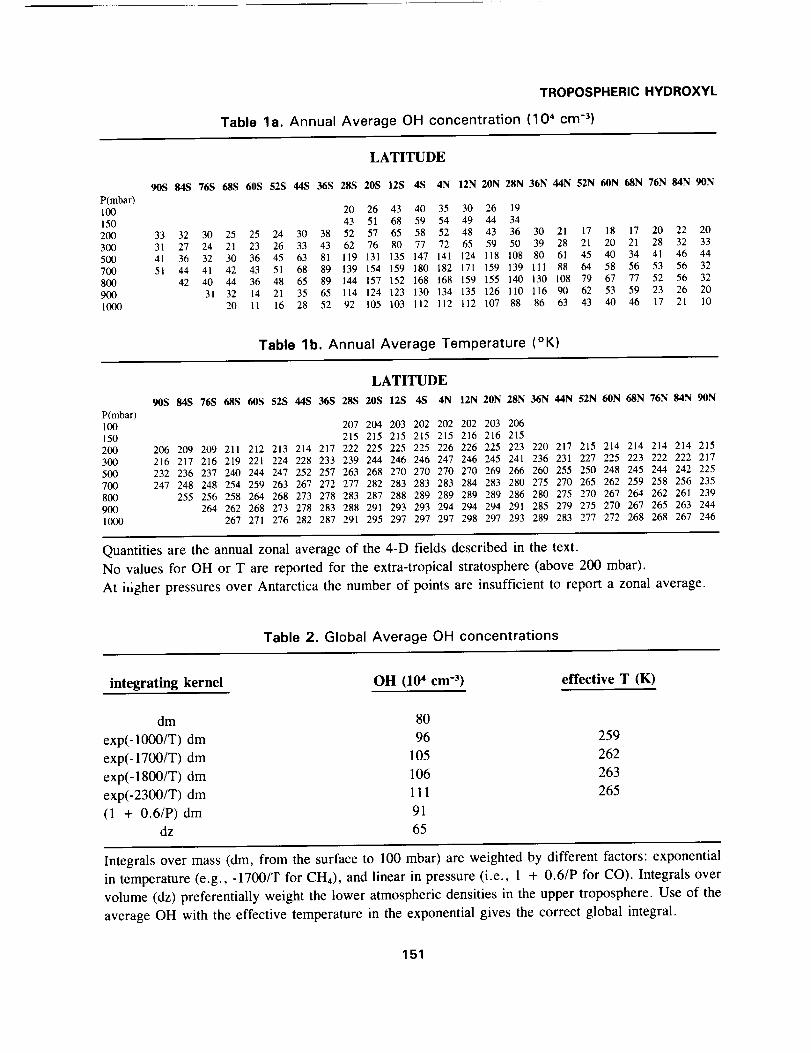
The annual averages of the zonal mean OH concentrations are shown in Table la; Table lb gives the

corresponding annual average temperatures. Hydroxyl concentrations are highest in the middle troposphere

over the tropics. The OH density peaks at 700-800 mbar because cloud cover and Rayleigh scatteringreduce solar ultraviolet light below 800 mbar.

The global loss of a gas that reacts with OH is the integral over a wide range of conditions in tempera-

ture, density and trace gas abundance. The integrand is extremely non-linear, and thus, the average loss

150


Table l a. AnnualAverageOH concentration(104cm"_)

LATITUDE

90S 84S 76S 68S 60S 52S 44S 36S 28S 20S 12S 4S 4N 12N 20N 28N 36N 44N 52N 60N 68N 76N 84N 90N

P(mbar)100 20 26 43 40 35 30 26 19

150 43 51 68 59 54 49 44 34200 33 32 30 25 25 24 30 38 52 57 65 58 52 48 43 36 30 21 17 18 17 20 22 20

300 31 27 24 21 23 26 33 43 62 76 80 77 72 65 59 50 39 28 21 20 21 28 32 33

500 41 36 32 30 36 45 63 81 119 131 135 147 141 124 118 108 80 61 45 40 34 41 46 44

700 51 44 41 42 43 51 68 89 139 154 159 180 182 171 159 139 111 88 64 58 56 53 56 32

800 42 40 44 36 48 65 89 144 157 152 168 168 159 155 140 130 108 79 67 77 52 56 32

900 31 32 14 21 35 65 114 124 123 130 134 135 126 110 116 90 62 53 59 23 26 20

1000 20 11 16 28 52 92 105 103 112 112 112 107 88 86 63 43 40 46 17 21 10

Table lb, Annual Average Temperature (°K)

LATITUDE

90S 84S 76S 68S 60S 52S 44S 36S 28S 20S 12S 4S 4N 12N 20N 28N

P(mbar)1(30 207 204 203 202 202 202 203 206150 215 215 215 215 215 216 216 215

200 206 209 209 211 212 213 214 217 222 225 225 225 226 226 225 223

300 216 217 216 219 221 224 228 233 239 244 246 246 247 246 245 241

500 232 236 237 240 244 247 252 257 263 268 270 270 270 270 269 266

700 247 248 248 254 259 263 267 272 277 282 283 283 283 284 283 280

800 255 256 258 264 268 273 278 283 287 288 289 289 289 289 286

900 264 262 268 273 278 283 288 291 293 293 294 294 294 291

1000 267 271 276 282 287 291 295 297 297 297 298 297 293

36N 44N 52N 60N 68N 76N 84N 90N

220 217 215 214 214 214 214 215

236 231 227 225 223 222 222 217260 255 250 248 245 244 242 225

275 270 265 262 259 258 256 235

280 275 270 267 264 262 261 239

285 279 275 270 267 265 263 244

289 283 277 272 268 268 267 246

Quantities are the annual zonal average of the 4-D fields described in the text.

No values for OH or T are reported for the extra-tropical stratosphere (above 200 mbar).

At ifigher pressures over Antarctica the number of points are insufficient to report a zonal average.

Table 2. Global Average OH concentrations

integrating kernel OH (10 4 cm "3) effective T (K)

dm 80

exp(- 1000/T) dm 96

exp(-1700/T) dm 105

exp(-1800/T) dm 106

exp(-2300/T) dm 111

(1 + 0.6/P) dm 91dz 65

259

262

263

265

Integrals over mass (dm, from the surface to 100 mbar) are weighted by different factors: exponential

in temperature (e.g., -1700/T for cn4), and linear in pressure (i.e., 1 + 0.6/P for CO). Integrals over

volume (dz) preferentially weight the lower atmospheric densities in the upper troposphere. Use of the

average OH with the effective temperature in the exponential gives the correct global integral.

151


is not equal simply to the product of averages (Makide and Rowland, 1981). It is misleading to report

a single "global average OH concentration" without qualifying it as to the averaging kernel. The global

OH concentrations averaged over the atmosphere (100-1000 mbar with no stratospheric contribution) are

reported here in Table 2 for a variety of integrating kernels. The average OH is largest, 11 lxl04 cm -3,

when weighted appropriately (by mass) for loss of an HCFC with a large exponential factor of-2300/T.

A larger temperature dependence result in greater average OH because the OH densities are maximal at

high temperatures in the tropics (see Table 1). The spatially averaged OH density is smallest, 65x 104 cm -3,

because of the large volumes of air in the upper troposphere with low OH concentrations. The effective

temperatures given in Table 2 are those needed to get the correct globally averaged integral, and should

not be confused with the optimal scaling temperature in Section 4. (The scaling temperature must also

account for the change in mean OH as the temperature dependence varies.)

3. GLOBAL LOSS OF CH3CCI_ AND CH4

The globally integrated losses for methane and for methyl chloroform are calculated by integrating the

loss frequency (OH and temperature fields described above) using realistic, but fixed tropospheric distri-

butions for CH4 and CH3CC13. Tropospheric reactions with OH dominate the loss of both species, but

stratospheric losses cannot be ignored and are used in place of OH densities in layer 9 (0-70 mbar) global-

ly and in layer 8 (70-150 mbar) outside the tropics. The stratospheric losses are calculated from a 1-D

vertical diffusion model for stratospheric chemistry evaluated at the appropriate latitude and season.

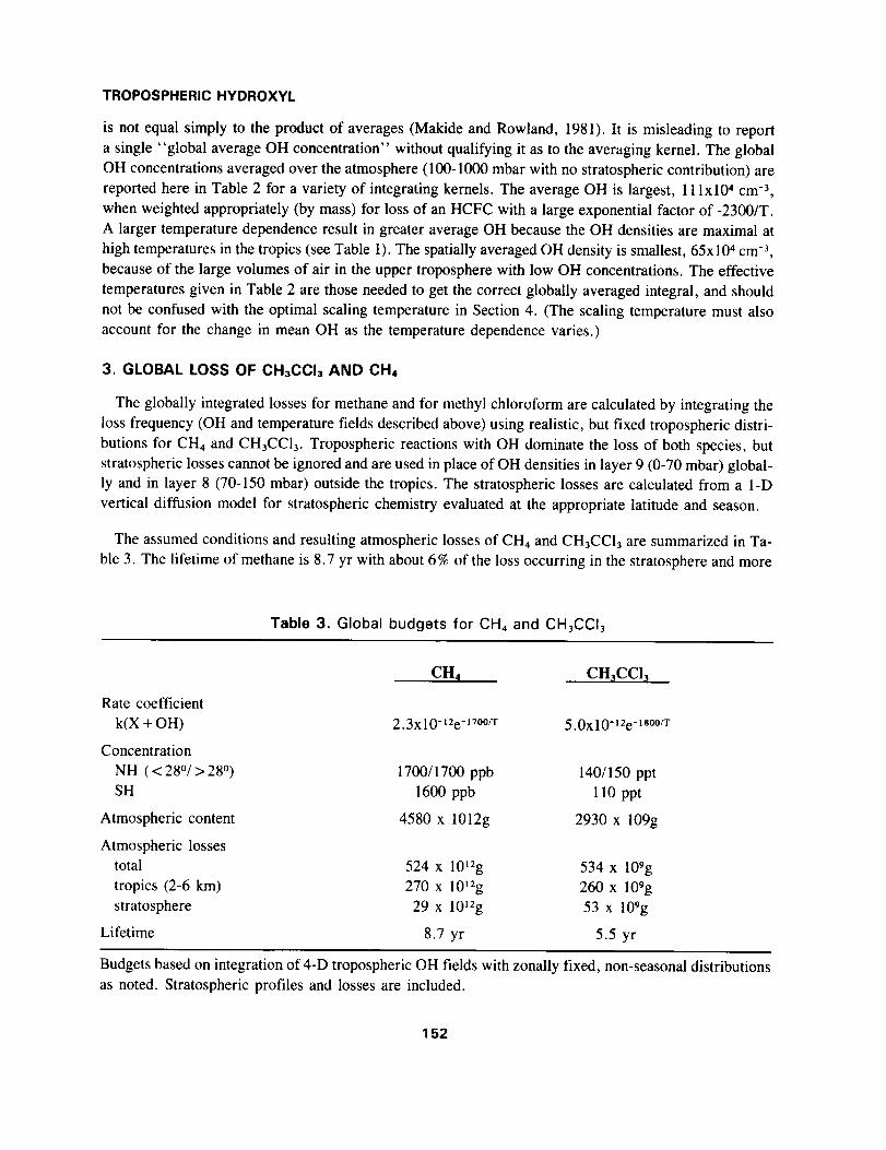
The assumed conditions and resulting atmospheric losses of CH4 and CH3CCI3 are summarized in Ta-

ble 3. The lifetime of methane is 8.7 yr with about 6 % of the loss occurring in the stratosphere and more

Table 3. Global budgets for CH4 and CH3CCI3

CH4 CH3CCIj

Rate coefficient

k(X + OH) 2.3xl0-t2e-17°°/T 5.0xl0-12e -lsoo/T

Concentration

NH ( <28°/>28 °) 1700/1700 ppb 140/150 ppt

SH 1600 ppb 110 ppt

Atmospheric content 4580 x 1012g 2930 x 109g

Atmospheric losses

total 524 x 1012g 534 x 109g

tropics (2-6 krn) 270 x 10_2g 260 x 109g

stratosphere 29 x 1012g 53 x 109g

Lifetime 8.7 yr 5.5 yr

Budgets based on integration of 4-D tropospheric OH fields with zonally fixed, non-seasonal distributions

as noted. Stratospheric profiles and losses are included.

152


than half in the tropical middle troposphere. The lifetime of methyl chloroform is 5.5 yr. Stratospheric

loss for methyl chloroform is about three times more rapid than for methane because photolysis of CH3CCI 3

becomes important in the stratosphere. Again the tropical middle troposphere accounts for about half of

the global loss.

Methyl chloroform is usually chosen as a reference species for tropospheric loss, with a "known" at-

mospheric lifetime based on the ALE/GAGE analysis of Prinn et al. (1987). We compare the lifetimes

in Table 3 for CH3CC13 with those from the ALE/GAGE analysis and the recent 3-D CTM simulations

(Spivakovsky et al, 1989). The ALE/GAGE analysis uses observations of CH3CCI 3 at 5 surface sites,

industry data for atmospheric emissions, and a 9-box atmospheric model, to derive an annual average

global lifetime of 6.3 yr with a reported 1-sigma range of 5.4-7.5 yr. Errors in the lifetime due to uncer-

tainties in the atmospheric emissions used in the ALE/GAGE study have been reduced by recent analyses

of CHaCCI3 sources from industry surveys (Midgley, 1989) and from observations (Prather, 1988).

When the same OH and temperature fields are used in the complete CTM simulation of CH3CC13

(Spivakovsky et al., 1989) the integrated loss correctly includes all correlations of OH and temperature

with CH3CC13 concentrations. The 3-D CTM simulation showed that the standard OH field (with a result-

ing lifetime of 5.5 yr) and the OH field scaled by a factor of 0.75 (with a lifetime of 7.1 yr) bracket the

observations. This range, however, does not include uncertainties in the observations (i.e., absolute calibra-

tion) or in the sources. The observed seasonal cycle of CH3CCI3 in the southern hemisphere is not a direct

measure of the absolute OH concentrations; however, its accurate simulation in the CTM provides some

confirmation of the integrated seasonal variation of the modeled OH fields in the southern hemisphere.

Such comparisons emphasize the mid-latitude photochemistry which has the largest seasonal variations,

and they are independent of absolute calibration and sources because they depend on the relative (%) changes

in CH3CC13.

It is difficult to find other globally distributed trace gases with well defined sources and trends that can

be used to test global OH concentrations. For example, Derwent and Volz-Thomas (AFEAS, May, 1989;

Volz et al., 1981) have used carbon monoxide, both _4CO and _2CO, to test and recalibrate the OH fields

in their 2-D model. Another possibility, HCFC-22 (CHF2C1) has limited data on hemispheric abundances,

trends and sources. Data for HCFC-22 are sparse and barely able to define the hemispheric ratio and in-

stantaneous trend (N/S = 89/77 ppt, + 6.5 ppt/yr in 1985, see NASA/WMO, 1986). Furthermore, sig-

nificant uncertainties exist currently for the absolute calibration and atmospheric emissions of most HCFCs.

HCFC-22 is used as an intermediate chemical in the production of other compounds, and thus its release

is only a fraction of production. Recent estimates of HCFC-22 emission (130 Gg/yr in 1985, M. McFarland,

personal communication) are twice as large as previous values, and are now barely able to reconcile the

current atmospheric budget from the limited observations noted above.

It is not possible at present to put a formal "one-sigma" accuracy on the OH fields used here, either

from first principles, or from constraints using the methyl chloroform budget. The uncertainty factor for

the OH fields is chosen to be 1.3 and is applied to the lifetimes for HCFCs in Section 5.

153


4. SENSITIVITYOF HCFCLIFETIME TO GLOBAL DISTRIBUTION

We use the 4-D fields of OH and temperature to understand how to predict the lifetime of one species

relative to another. Specifically, how can the lifetime of one species be scaled to another with a different

spatial-temporal distribution and loss rate? Idealized tropospheric distributions are used to examine the

sensitivity of HCFC lifetime to (a) the temperature dependence of their reaction rates with OH, (b) large

interhemispheric gradients, (c) enhanced concentrations in the boundary layer near sources, and (d) seasonal

cycles in concentration.

a. Sensitivity to rate coefficient: k = A x exp(-B/T)

Two species, X and Y, with the same global distribution and with rate coefficients for reaction with

OH that differ only by a constant factor, k(OH + X)/k(OH + Y) = constant, will have lifetimes that scale

inversely by the same factor. In most cases, however, the rate coefficients have different temperature de-

pendence, B, or pressure dependence (as in the case of CO). We investigate the dependence of HCFC

lifetime on values of B ranging from 0 to 2300 K, by integrating the loss for an atmospheric tracer that

is uniformly distributed throughout the troposphere and stratosphere. The A coefficient was selected to

match the CH4 rate, k = 2.3E-12 x exp(-B/T) cm 3 s-l, and stratospheric losses were not included.

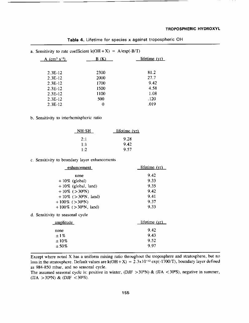
The integrated global loss rates are given in Table 4a; lifetimes range from 81 yr (B = 2300 K) to

0.02 yr (B = 0 K). In Figure 1 we show the error associated with predicting the lifetime by scaling to

a reference lifetime (9.42 yr at B = 1700 K) using an appropriate temperature in the ratio of reaction

rates. This scaling temperature is not necessarily the mean temperature of the OH losses, but includes

also the shift in the reaction-weighted mean OH as a function of reaction rate (see Section 2 and Table

2). The optimal temperature for scaling the lifetimes is 277 K, and the resulting errors are less than 2 %

over the range 800 K < B < 2300 K. Use of a temperature 10 K warmer or colder yields errors in the

lifetime of order 10% when scaling the reference case (B = 1700 K) to greater (2300 K) or smaller (1000

K) activation energies.

b. Sensitivity to interhemispheric gradient

HCFCs released predominantly from industrialized countries in the northern mid-latitudes will estab-

lish a global distribution similar to that for CFCs (see Prather et al., 1987). The north-to-south latitudinal

gradient will have an interhemispheric absolute difference about equal to one year's emissions, and higher

concentrations will build up over the presumed continental sources at mid-latitudes. The sensitivity of

HCFC lifetimes to their interhemispheric gradient will depend on hemispheric asymmetries in the OH

fields (and temperatures in so far as they affect the rate coefficients). The base case described above as-

sumes a uniformly distributed tracer with OH reaction rates appropriate for CH4, and the perturbed case

includes doubling the abundance in either hemisphere uniformly. Results are shown in Table 4b. For a

factor of 2 asymmetry in the HCFC distribution, the lifetime changes by only 1.5%. Thus the effective

OH loss is about 9% greater in the northern hemisphere. Spivakovsky et al. (1989) note that the higher

concentrations of CO in the northern hemisphere (reducing OH) are more than offset by the higher levels

of 03 and NO x.

154


Table4. Lifetime for speciesx against troposphericOH

a. Sensitivity to rate coefficient k(OH + X) = A/exp(-B/T)

A (cm a s-1) B (K) lifetime (yr)

2.3E-12 2300 81.2

2.3E-12 2000 27.7

2.3E-12 1700 9.42

2.3E-12 1500 4.582.3E-12 1100 1.08

2.3E-12 500 .120

2.3E-12 0 .019

b. Sensitivity to interhemispheric ratio

NH:SH lifetime (yr)

2:1 9.28

1:1 9.42

1:2 9.57

c. Sensitivity to boundary layer enhancements

enhancement

none

+ 10% (global)

+ 10% (global, land)+ 10% ( > 30°N)

+ 10% (>30°N, land)+ 100% (>30°N)

+ 100% (>30°N, land)

d. Sensitivity to seasonal cycle

amplitude

none

_+1%_+10%

_+50%

lifetime (yr)

9.42

9.33

9.35

9.42

9.41

9.379.33

lifetime (vr)

9.42

9.43

9.52

9.97

Except where noted X has a uniform mixing ratio throughout the troposphere and stratosphere, but no

loss in the stratosphere. Default values are k(OH + X) = 2.3x10 -_2 exp(-1700/T), boundary layer defined

as 984-850 mbar, and no seasonal cycle.

The assumed seasonal cycle is: positive in winter, (DJF >30°N) & (JJA <30°S), negative in summer,(JJA >30°N) & (DJF <30°S).

155


40

30

20

10

0

-10

-20

v_

% ERROR BY SCALING" k A exp (-B/T)

..o= T = 267T = 277

-v- T = 287

-_-'_'= _/'-'= -= ,2"_00 230A --_-'- -"()

1500 1700 _,,, -, -.

B=O

5OO

q I L

.01 .1 1 10

Lifetime (yr)

100

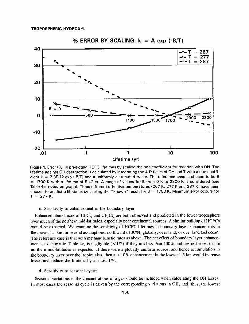
Figure 1. Error (%) in predicting HCFC lifetimes by scaling the rate coefficient for reaction with OH. The

lifetime against OH destruction is calculated by integrating the 4-D fields of OH and T with a rate coeffi-

cient k = 2.3E-12 exp (-B/T) and a uniformly distributed tracer. The reference case is chosen to be B

= 1700 K with a lifetime of 9.42 yr. A range of values for B from 0 K to 2300 K is considered (see

Table 4a, noted on graph). Three different effective temperatures (267 K, 277 K and 287 K) have beenchosen to predict a lifetimes by scaling the "known" result for B = 1700 K. Minimum error occurs forT = 277 K.

c. Sensitivity to enhancement in the boundary layer

Enhanced abundances of CFC13 and CF2C12 are both observed and predicted in the lower troposphere

over much of the northern mid-latitudes, especially near continental sources. A similar buildup of HCFCs

would be expected. We examine the sensitivity of HCFC lifetimes to boundary layer enhancements in

the lowest 1.5 km for several assumptions: northward of 30°N, globally, over land, or over land and ocean.

The reference case is that with methane kinetic rates as above. The net effect of boundary layer enhance-

ments, as shown in Table 4c, is negligible (< 1%) if they are less than 100% and are restricted to the

northern mid-latitudes as expected. If there were a globally uniform source, and hence accumulation in

the boundary layer over the tropics also, then a + 10% enhancement in the lowest 1.5 km would increase

losses and reduce the lifetime by at most 1%.

d. Sensitivity to seasonal cycles

Seasonal variations in the concentrations of a gas should be included when calculating the OH losses.

In most cases the seasonal cycle is driven by the corresponding variations in OH, and, thus, the lowest

156


concentrations of the trace gas occur slightly after the greatest OH levels (i.e., late summer). This an-

ticorrelation of OH and trace gas increases the lifetime of the gas relative to that calculated with a fixed

concentration. As shown in Table 4d, this effect is negligible (<0.2%) for a gas like CH4 with a lifetime

of about 9 yr and an observed seasonal amplitude of + 1.5 %. Since large seasonal variations occur only

in short-lived species, we would not expect the seasonal amplitude for an HCFC to exceed _+10% (cor-

responding to a 1% increase in lifetime) unless the lifetime were very short, less than 1.5 yr. The seasonal

effect is so small because the majority of OH loss occurs in the tropics, as noted above, where OH concen-

trations do not vary significantly with season.

In summary, a short-lived HCFC with a lifetime of about 0.5 yr might be expected to have a seasonal

amplitude of + 25 % (lifetime correction: + 2.5 %), a north:south interhemispheric ratio of 2:1 (lifetime

correction: -1.5 %), and a boundary layer enhancement north of 30°N over land of 100% (lifetime correc-

tion: -1%). The sum of these corrections tend to cancel, or be very small, and thus the lifetime predicted

from a uniform distribution should be a reasonably accurate, _+10%, evaluation of the true lifetime.

5. SUMMARY OF HCFC LIFETIMES

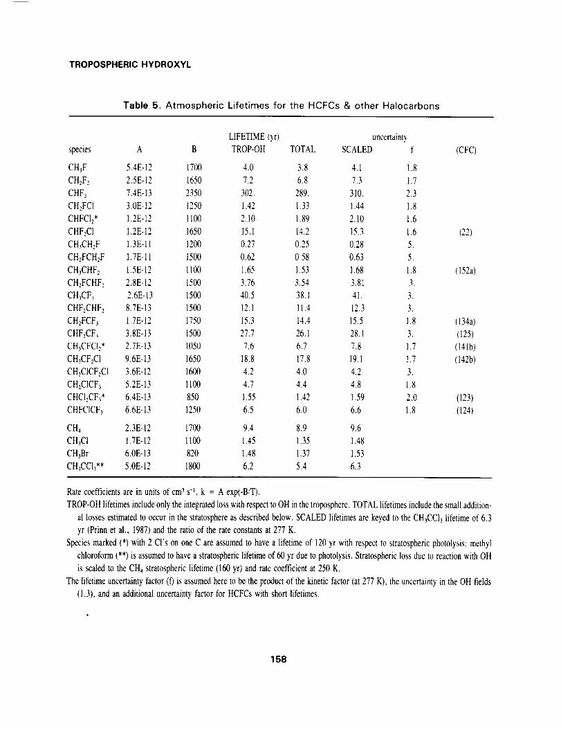
The lifetimes of HCFCs and other hydrohalocarbons are reported in Table 5. These lifetimes are calcu-

lated directly from the tropospheric OH fields using the recommended rate coefficients (Hampson, Kurylo

and Sander, AFEAS, 1989) and a fixed, uniform distribution of trace gas (labelled TROP-OH). They

have been augmented (labelled TOTAL) with much smaller stratospheric losses that include estimated

destruction by OH and photolysis. Stratospheric OH loss is scaled by rate coefficients at a temperature

of 250 K to an assumed methane (stratosphere only) loss rate of 1/160 yr-I; stratospheric photolysis is

assumed only for species with a -CCI3 group (1/60 yr -_) or a -CC12 group (1/120 yr -I) and is based on

the lifetimes of CFCI3 and CF2C12. An additional column of lifetimes in Table 5 (labelled SCALED) has

been calculated by ratioing the rate coefficients (scaling temperature of 227 K) and multiplying by the

methyl chloroform lifetime of 6.3 yr. As expected from the analyses in this report the two approaches

agree very well.

An attempt has been made to estimate uncertainty factors for HCFC lifetimes in the same manner as

in the kinetics reviews. We identify the uncertainty in the reaction rate of 277 K and then multiply by

the estimated uncertainty factor for the OH fields (1.3). The uncertainty associated with a non-uniform

distribution is significant only for HCFCs with lifetimes less than 1 yr, and has been increased. The final

uncertainty quoted in Table 5 is representative of the likely range, but cannot be treated as a formal statistical

error.

Although the ALE/GAGE analysis of the total atmospheric residence time for CH3CC13 agrees with

the chemical model's lifetime for destruction by OH, the combined uncertainties in the two lifetimes can-

not rule out another sink, such as hydrolysis (Wine and Chameides, AFEAS, 1989), with a lifetime as

short as 25 yr.

There is a clear need for other trace species that can be used to test the tropospheric abundance of OH.

Such species must have accurate histories of emissions and good, absolutely calibrated measurements.

In situ atmospheric tests of the kinetic model for OH should possibly focus on the tropical middle tropospherewhere most of the destruction of HCFCs will occur.

157


Table 5. Atmospheric Lifetimes for the HCFCs & other Halocarbons

LIFETIME(yr) uncertainty

species A B TROP-OH TOTAL SCALED f (CFC)

CH3F 5.4E-12 1700 4.0 3.8 4.1 1.8

CH2F2 2.5E-12 1650 7.2 6.8 7.3 1.7

CHF3 7.4E-13 2350 302. 289. 310. 2.3

CH2FCI 3.0E-12 1250 1.42 1.33 1.44 1.8

CHFClz* 1.2E-12 1100 2.10 1.89 2.10 1.6

CHF:C1 1.2E-12 1650 15.1 14.2 15.3 1.6 (22)

CH3CHzF 1.3E-11 1200 0.27 0.25 0.28 5.

CH2FCH2F I.TE-1l 1500 0.62 0,58 0.63 5.

CHsCHF2 1.5E-12 1100 1.65 1.53 1.68 1.8 (152a)

CH2FCHF: 2.8E-12 1500 3.76 3.54 3.81 3.

CH3CF3 2.6E-13 1500 40.5 38. l 41. 3.

CHF2CHF2 8.7E-13 1500 12.1 11.4 12.3 3.

CH2FCF3 1.7E-12 1750 15.3 14.4 15.5 1.8 (134a)

CHF:CF3 3.8E-13 1500 27.7 26.1 28.1 3. (125)

CH3CFCh* 2.7E-13 1050 7.6 6.7 7.8 1.7 (141b)

CH3CF2CI 9.6E-13 1650 18.8 17.8 19.1 1.7 (142b)

CH2CICF2CI 3.6E-12 1600 4.2 4.0 4.2 3.

CH2CICF3 5.2E-13 l l00 4.7 4.4 4.8 1.8

CHCIzCF3* 6.4E-13 850 1.55 1.42 1.59 2.0 (123)

CHFC1CF3 6.6E-13 1250 6.5 6.0 6.6 1.8 (124)

CH4 2.3E-12 1700 9.4 8.9 9.6

CH3CI 1.7E-12 1100 1.45 1.35 1.48

CH3Br 6.0E-13 820 1.48 1.37 1.53

CH3CCI3** 5.0E-12 1800 6.2 5.4 6.3

Rate coefficientsare in units of cm3 s-_, k = A exp(-B/T).

TROP-OHlifetimesincludeonly the integratedlosswithrespecttoOH inthe troposphere.TOTALlifetimesincludethe smalladdition-

al losses estimatedto occur in the stratosphereas described below. SCALEDlifetimesare keyed to the CH3CCI3lifetimeof 6.3

yr (Prinn et al., 1987)and the ratio of the rate constantsat 277 K.

Species marked (*) with 2 Cl's on one C are assumedto have a lifetimeof 120 yr with respect to stratosphericphotolysis; methyl

chloroform (**) is assumedto havea stratospheric lifetimeof 60 yr due to photolysis. Stratosphericloss due to reaction withOH

is scaled to the CH4stratospheric lifetime (160 yr) and rate coefficientat 250 K.

The lifetimeuncertaintyfactor (f) is assumedhere to be the productof the kinetic factor (at 277 K), the uncertaintyin the OH fields

(1.3), and an additionaluncertainty factor for HCFCs with short lifetimes.

158

Documents

TROPOSPHERIC OH AND HCFC/HFC - Earth System …€¦ · VO TROPOSPHERIC OH AND HCFC/HFC ... Future changes in the oxidative capacity of ... and chemical removal processes which involve