Embed Size (px)
Citation preview

1
True Online Temporal-Difference Learning(and Dutch Traces)
Harm van SeijenResearch Scientist, Maluuba

joint work with
Rupam Mahmood
Patrick Pilarski
Marlos Machado
Rich Sutton

part 1: why reinforcement learning?part 2: true online temporal-difference learningpart 3: effective multi-step learning for non-linear FA
Outline
3

natural language understanding
state tracker
policy managernatural language
generationdata
“Hi, do you know a good Indian restaurant”
system response
user act
systemact
dialogue stateuse
The central question: how to train the policy manager?
inform(food=“Indian”)
user input
“Sure. What price range are you thinking of?” request(price_range)
motivating example for RL
4
what is RL
Reinforcement Learning is a data-driven approach towards learning behaviour.
machine learning
unsupervised learning
supervised learning
reinforcement learning
+ + +=
deep reinforcement learning
deep learning deep learning deep learning
+ + +
5
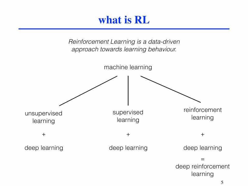
RL vs supervised learning
+
example: recognizing cats in images
f cat / no cat
behaviour: function that maps environment states to actions
supervised learninghard to specify function easy to identify correct output
6
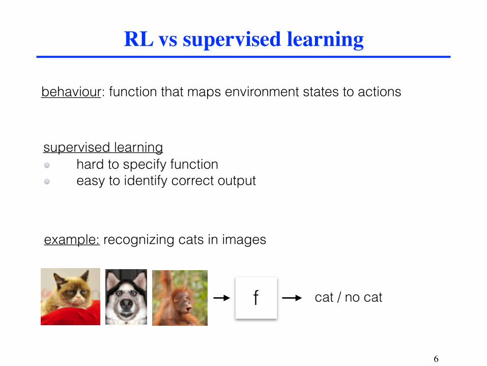
RL vs supervised learning
+
reinforcement learning: hard to specify function hard to identify correct output easy to specify behaviour goal
example: double inverted pendulum
state: θ1, θ2, ω1, ω2 action: clockwise/counter-clockwise torque on top joint goal: balance pendulum upright
behaviour: function that maps environment states to actions
7

advantages RL
+
does not require knowledge of good policy does not require labelled data online learning: adaptation to environment changes
8
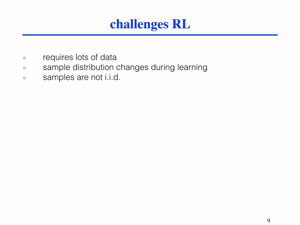
challenges RL
+
requires lots of data sample distribution changes during learning samples are not i.i.d.
9
part 1: why reinforcement learning?part 2: true online temporal-difference learningpart 3: effective multi-step learning for non-linear FA
Outline
10
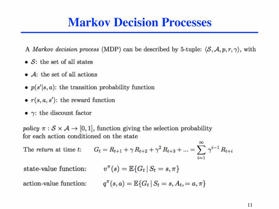
Markov Decision Processes
11
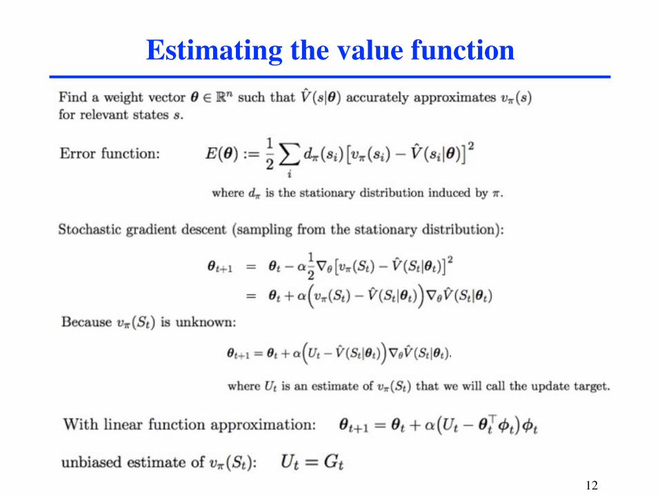
Estimating the value function
12
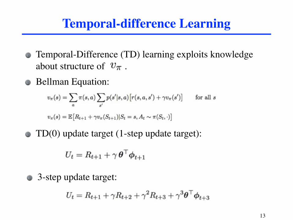
Temporal-Difference (TD) learning exploits knowledge about structure of .
Temporal-difference Learning
13
Bellman Equation:
TD(0) update target (1-step update target):
3-step update target:

update equations for linear function approximation:
TD(λ)
14
TD(λ) is a multi-step method, even though the update target looks like a 1-step update target.
This update is different from the general TD update rule.

the λ-return algorithm:
theorem*: for small step-sizes, computed by TD(λ) is approximately the same as computed by the λ-return algorithm.
the traditional forward view of TD(λ)
15
*see: Bertsekas, D. P. and Tsitsiklis, J. N. (1996). Neuro-Dynamic Programming.
note:
λ controls a trade-off between variance and bias of the update target, in general the best value of λ will differ from domain to domain.
How to set λ?
16
λ not only influences the speed of convergence, but in case of function approximation it also influences the asymptotic performance.
theoretical results for TD(λ) (Peter Dayan, 1992): - for λ = 1: convergence to LMS solution
- for λ < 1: convergence to a different fixed point

online method: the value of each visited state is updated at the time step immediately after the visit.offline method: the value of each visited state is updated at the end of an episode.
online vs offline methods
17
Is it possible to construct an online version of the λ-returnalgorithm that approximates TD(λ) at all time steps?
TD(λ) is an online method; the traditional λ-return algorithm is an offline method.

To compute , no data beyond time t should be used.At the same time, we want to have multi-step update targets that look many time steps ahead.
the challenge of an online forward view
True Online Temporal-Difference Learning
Algorithm 1 accumulate TD(�)
INPUT: ↵,�, �,✓init
✓ ✓init
Loop (over episodes):obtain initial �e 0While terminal state has not been reached, do:
obtain next feature vector �0 and reward R� R + � ✓>�0 � ✓>�e ��e + �✓ ✓ + ↵�e� �0
on simple tasks with bounded rewards. For this reason, a variant of TD(�) is often usedthat is more robust with respect to these parameters. This variant, which assumes binaryfeatures, uses a di↵erent trace-update equation:
et
(i) =
(��e
t�1(i) if �t
(i) = 0
1 if �t
(i) = 1for all features i .
This is referred to as the replacing-trace update. In this article, we use a simple generaliza-tion of this update rule that allows us to apply it to domains with non-binary features aswell:
et
(i) =
(��e
t�1(i) if �t
(i) = 0
�t
(i) if �t
(i) 6= 0for all features i . (6)
Note that for binary features this generalized trace update reduces to the default replacing-trace update. We will refer to the version of TD(�) that uses Equation 6 as ‘replace TD(�)’.
3.2 True Online TD(�)
✓t
The true online TD(�) update equations are:
�t
= Rt+1 + �(✓t
t
)>�t+1 � (✓t
t
)>�t
(7)
et
= ��et�1 + �
t
� ↵��[e>t�1�t
]�t
(8)
✓t+1t+1 = (✓t
t
) + ↵�t
et
+ ↵[(✓t
t
)>�t
� (✓t�1t�1)
>�t
][et
� �t
] (9)
for t � 0, and with e�1 = 0. Compared to accumulate TD(�) (equations (3), (4) and(5)), both the trace update and the weight update have an additional term. We call atrace updated in this way a dutch trace; we call the term ↵[✓>
t
�t
� ✓>t�1�t
][et
� �t
] theTD-error time-step correction, or simply the �-correction. Algorithm 2 shows pseudocodethat implements equations (7), (8) and (9).1
1. We provide pseudocode for true online TD(�) with time-dependent step-size in Section 7.1. For reasonsexplained in that section, this requires a modified trace update. In addition, for reference purposes, weprovide pseudocode for the special case of tabular features in Section 7.3.
5
the trick:
Use update targets that grow with the data-horizon.
18

normal update targets:
interim update targets:
interim update target
19
van Seijen, Mahmood, Pilarski, Machado, Sutton
experiments over a wide range of domains. Our extensive results support this hypothesis.In terms of computational cost, TD(�) has a slight advantage. In the worst case, true onlineTD(�) is twice as expensive. In the typical case of sparse features, it is only fractionally moreexpensive than TD(�). Memory requirements are the same. In terms of learning speed, trueonline TD(�) was often better, but never worse than TD(�) with either accumulating orreplacing traces, across all domains/representations that we tried. Our analysis showed thatespecially on domains with relatively low stochasticity and frequent revisits of features alarge di↵erence in learning speed can be expected. Furthermore, true online TD(�) has theadvantage over TD(�) with replacing traces that it can be used with non-binary features,and it has the advantage over TD(�) with accumulating traces that it is less sensitive withrespect to its parameters. Finally, we outlined an approach for deriving new true onlinemethods, based on rewriting the equations of a real-time forward view. This may lead tonew, interesting methods in the future.
9. Acknowledgements
The authors thank Hado van Hasselt for extensive discussions leading to the refinementof these ideas. This work was supported by grants from Alberta Innovates TechnologyFutures and the National Science and Engineering Research Council of Canada. Computingresources were provided by Compute Canada through WestGrid.
�t
! Ut
28
van Seijen, Mahmood, Pilarski, Machado, Sutton
experiments over a wide range of domains. Our extensive results support this hypothesis.In terms of computational cost, TD(�) has a slight advantage. In the worst case, true onlineTD(�) is twice as expensive. In the typical case of sparse features, it is only fractionally moreexpensive than TD(�). Memory requirements are the same. In terms of learning speed, trueonline TD(�) was often better, but never worse than TD(�) with either accumulating orreplacing traces, across all domains/representations that we tried. Our analysis showed thatespecially on domains with relatively low stochasticity and frequent revisits of features alarge di↵erence in learning speed can be expected. Furthermore, true online TD(�) has theadvantage over TD(�) with replacing traces that it can be used with non-binary features,and it has the advantage over TD(�) with accumulating traces that it is less sensitive withrespect to its parameters. Finally, we outlined an approach for deriving new true onlinemethods, based on rewriting the equations of a real-time forward view. This may lead tonew, interesting methods in the future.
9. Acknowledgements
The authors thank Hado van Hasselt for extensive discussions leading to the refinementof these ideas. This work was supported by grants from Alberta Innovates TechnologyFutures and the National Science and Engineering Research Council of Canada. Computingresources were provided by Compute Canada through WestGrid.
�t
! Ut
�t
! U1t
, U2t
, U3t
, . . . , Uh
t
28
data-horizon: time step up to which data is observed

λ-return:
interim λ-return: replace all n-step returns with n > h-t with the (h-t)-step return
van Seijen, Mahmood, Pilarski, Machado, Sutton
123
T
time
…
…
1θ12θ13θ1
2θ23θ2
3θ3
Tθ1Tθ2
TθTTθ3
Figure 9: The weight vectors of the new forward view mapped to the earliest time that theycan be computed.
call this version of the �-return the interim �-return, and use the notation G�|ht
to indicate
the interim �-return depending on horizon h. G�|ht
can be written as follows:
G�|ht
= (1 � �)h�t�1X
n=1
�n�1G(n)t
+ (1 � �)1X
n=h�t
�n�1G(h�t)t
= (1 � �)h�t�1X
n=1
�n�1G(n)t
+ G(h�t)t
·h(1 � �)
1X
n=h�t
�n�1i
= (1 � �)h�t�1X
n=1
�n�1G(n)t
+ G(h�t)t
·h�h�t�1(1 � �)
1X
k=0
�k
i
= (1 � �)h�t�1X
n=1
�n�1G(n)t
+ �h�t�1G(h�t)t
(12)
Equation 12 fully specifies the interim �-return, except for one small detail: the weightvector that should be used for the value estimates in the n-step returns has not been specified
yet. The regular �-return uses G(n)t
(✓t
) (see Equation 10). For the real-time forward view,however, all weight vectors have two indices, so simply using ✓
t
does not work in this case.So which double-indexed weight vector should be used? The two guiding principles ondeciding which weight vector to use is that we want the forward view to be an approximationof accumulate TD(�) and that an e�cient implementation should be possible. One option
is to use G(n)t
(✓h
t
). While with this definition the update-sequence at data-horizon T isexactly the same as the sequence of updates from the �-return algorithm (basically, the�-return implicitly uses a data-horizon of T ), it prohibits e�ciently computation of ✓h+1
h+1
from ✓h
h
. For this reason, we use G(n)t
(✓t+n�1t+n�1), which does allow for e�cient computation,
and forms a good approximation of accumulate TD(�) as well (as we show below). Using
20
True Online Temporal-Difference Learning
6.1 The forward view of TD(�)
In Section 2, the general update rule for linear function approximation was presented (Equa-tion 1), which is based on the update rule for stochastic gradient descent. The updateequations for TD(�), however, are of a di↵erent form (Equations 3, 4 and 5). The forwardview of TD(�) relates the TD(�) equations to Equation 1. Specifically, the forward view ofTD(�) specifies that TD(�) approximates the �-return algorithm. This algorithm performsa series of updates of the form of Equation 1 with the �-return as update target:
✓t+1 = ✓
t
+ ↵ [G�
t
� ✓>t
�t
]�t
, for 0 t < T,
where T is the end of the episode, and G�
t
is the �-return at time t.The �-return is a multi-step update target based on a weighted average of all future
state values, with � determining the weight distribution. Specifically, the �-return at timet is defined as:
G�
t
= (1 � �)1X
n=1
�n�1G(n)t
(✓t
)
with G (n)t
(✓) is the n-step return, defined as:
G (n)t
(✓) = Rt+1 + �R
t+2 + �2Rt+3 + · · · + �n�1R
t+n
+ �n ✓>�t+n
.
For episodic tasks, G (n)t
(✓) is equal to the full return, Gt
, if t + n � T , and the �-returncan be written as:
G�
t
= (1 � �)T�t�1X
n=1
�n�1G(n)t
(✓t
) + �T�t�1Gt
. (10)
The forward view o↵ers a particularly straightforward interpretation of the �-parameter.For � = 0, G�
t
reduces to the TD(0) update target, while for � = 1, G�
t
reduces to the fullreturn. In other words, for � = 0 the update target has maximum bias and minimumvariance, while for � = 1, the update target is unbiased, but has maximum variance. For �in between 0 and 1, the bias and variance are between these two extremes. So, � enablescontrol over the trade-o↵ between bias and variance.
While the �-return algorithm has a very clear intuition, there is only an exact equivalencefor the o✏ine case. That is, the o✏ine variant of TD(�) computes the same value estimatesas the o✏ine variant of the �-return algorithm. For the online case, there is only anapproximate equivalence. Specifically, the weight vector at time T , computed by accumulateTD(�) closely approximates the weight vector at time T computed by the online �-returnalgorithm for appropriately small values of the step-size parameter (Sutton and Barto,1998).
That the forward view only applies to the weight vector at the end of an episode, evenin the online case, is a limitation that is often overlooked. It is related to the fact that the�-return for S
t
is constructed from data stretching from time t+1 all the way to time T , thetime that the terminal state is reached. A consequence is that the �-return algorithm cancompute its weight vectors only in hindsight, at the end of an episode. This is illustratedby Figure 7, which maps each weight vector ✓
t
to the earliest time that it can be computed.‘Time’ in this case refers to the time of data-collection: time t is defined as the moment
17
interim λ-return
20
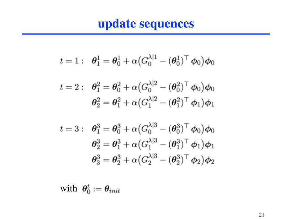
update sequences
21
with

online lambda-return algorithm.
22
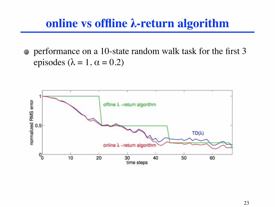
performance on a 10-state random walk task for the first 3 episodes (λ = 1, α = 0.2)
23
online vs offline λ-return algorithm
Theorem*
24
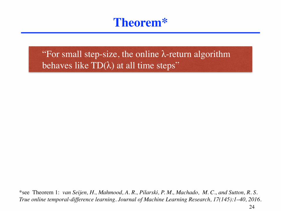
“For small step-size, the online λ-return algorithm behaves like TD(λ) at all time steps”
*see Theorem 1: van Seijen, H., Mahmood, A. R., Pilarski, P. M., Machado, M. C., and Sutton, R. S. True online temporal-difference learning. Journal of Machine Learning Research, 17(145):1–40, 2016.

λ = 1
Sensitivity of TD(λ) to Divergence
25
RMS error during early learning
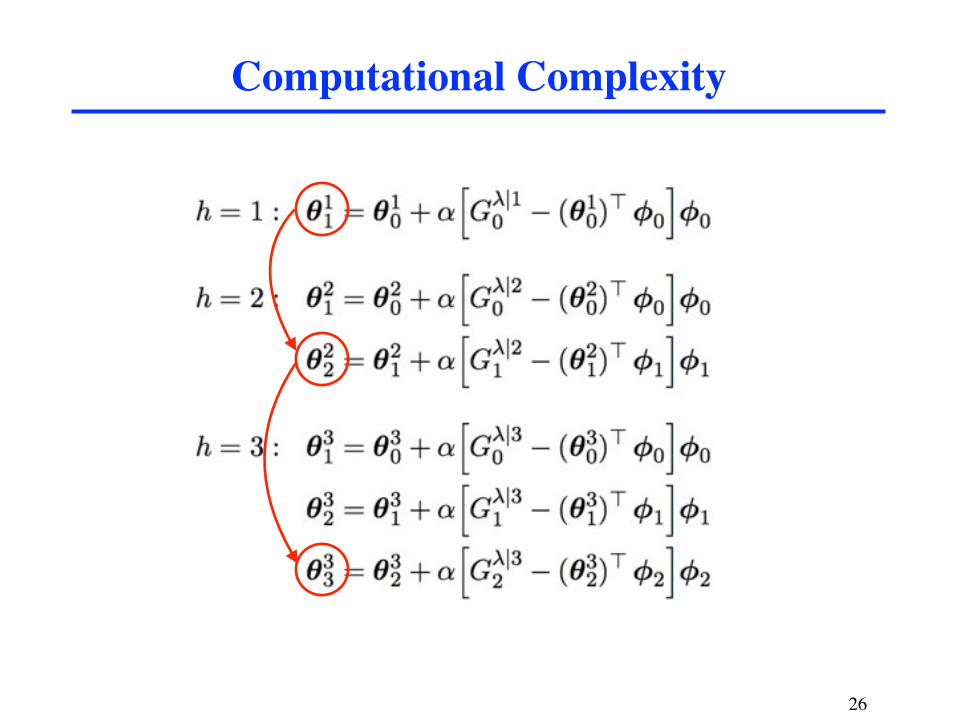
Computational Complexity
26
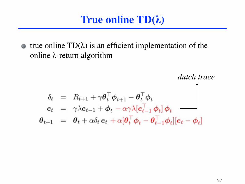
true online TD(λ) is an efficient implementation of the online λ-return algorithm
True online TD(λ)
27
dutch trace

Empirical Comparison
28
in all domains, true online TD(λ) performs at least as good as replace/accumulate TD(λ)
0
0.2
0.4
0.6
0.8
1
1.2
norm
aliz
ed e
rror
replace TD(λ) accumulate TD(λ) true online TD(λ)
(10, 3, 0.1)tabular
(10, 3, 0.1)binary
(10, 3, 0.1)non−binary
(100, 10, 0.1)tabular
(100, 10, 0.1)binary
(100, 10, 0.1)non−binary
(100, 3, 0)tabular
(100, 3, 0)binary
(100, 3, 0)non−binary
prostethicangle
prostethicforce

part 1: why reinforcement learning?part 2: true online temporal-difference learningpart 3: effective multi-step learning for non-linear FA
Outline
29
Implementing the online forward view is computationally very expensive.
Memory as well as computation time per time step grows over time.
In the case of linear FA there is an efficient backward view with exact equivalence: true online TD(λ).
Computational cost is span-independent and linear in the number of features.
In the case of non-linear FA such an efficient backward view does not appear to exist.
30
Computational Cost
New Research Question
31
Answer: Υes
Is it possible to construct a different online forward view, with a performance close to that of the online λ-return algorithm, that can be implemented efficiently?

Uses online λ-return with fixed horizon, K steps ahead:As a consequence, updates occur with a delay of K time steps.Computational cost is span-independent and efficient (computational complexity equal to TD(0)).
forward TD(λ)
32
0 10 20 30 40 50 600
0.5
1
time steps
norm
aliz
ed R
MS
erro
r
offline λ −return algorithm
forward TD(λ)
online λ −return algorithm
(K=15)
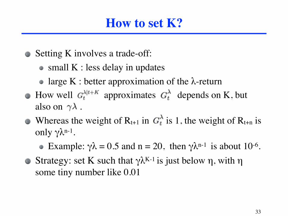
Setting K involves a trade-off:small K : less delay in updateslarge K : better approximation of the λ-return
How well approximates depends on K, but also on .Whereas the weight of Rt+1 in is 1, the weight of Rt+n is only γλn-1.
Example: γλ = 0.5 and n = 20, then γλn-1 is about 10-6.Strategy: set K such that γλK-1 is just below η, with η some tiny number like 0.01
How to set K?
33
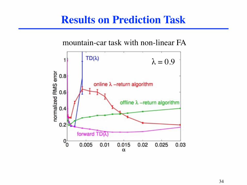
Results on Prediction Task
34
mountain-car task with non-linear FA
λ = 0.9
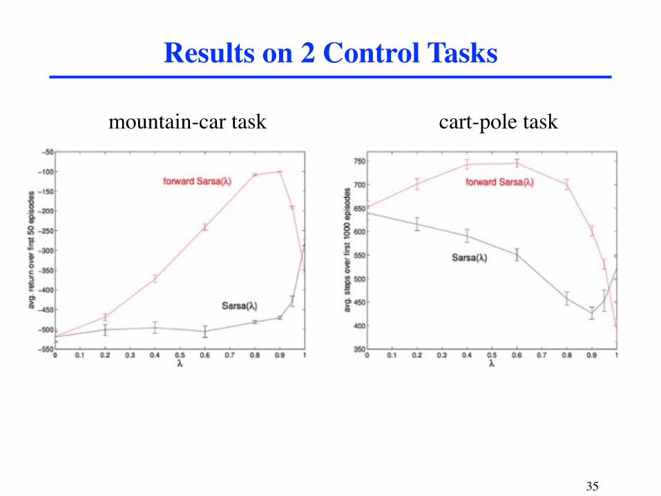
Results on 2 Control Tasks
35
mountain-car task cart-pole task

What about deep RL?
36
Question: can this technique be applied to DQN?
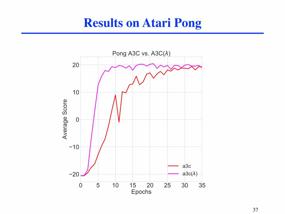
Results on Atari Pong
37

1. The online λ-return algorithm outperforms TD(λ), but is computationally very expensive.
2. For linear FA, an efficient backward view exists with exact equivalence: true online TD(λ).
3. For non-linear FA, such an efficient backward view does not appear to exist.
4. Forward TD(λ) approximates the online λ-return algorithm and can be implemented efficiently for non-linear FA.
5. The price that forward TD(λ) pays is a delay in the updates.6. Empirically, forward TD(λ) can outperform TD(λ) substantially
on domains with non-linear FA.7. The forward TD(λ) strategy does not work well with experience
replay with long histories, but it can be applied to A3C.
Summary
38
39
Thank you!
References: 1) van Seijen, H., Mahmood, A. R., Pilarski, P. M., Machado, M. C., and Sutton, R. S. True online temporal-difference learning. Journal of Machine Learning Research, 17(145):1–40, 2016. 2) van Seijen, H. Effective multi-step temporal-difference learning for non-linear function approximation. arXiv:1608.05151, 2016.