Embed Size (px)
Citation preview
Abstract— The paper presents the development of a wind turbine simulator which consists of an induction motor driven by a torque control inverter. The wind turbine simulation system includes: wind speed simulation, mathematical model of wind turbines, modeling of rotor blade characteristics, modeling of tower effect and emulation of rotor inertia. Wind speed can be easily programmed according to recorded wind speed data or Van Der Hoven model or manual set up. The developed algorithms were implemented by a low-cost, high-performance DSC controller with C language and the system was tested in the laboratory with 1 kW dc generator. The power responses, torque responses and tip speed ratio responses confirms that the system can operate very well under step change of power reference and load disturbances. The advantages of the simulators are that various wind profiles and wind turbines can be incorporated as desired in the control software and it includes the data acquisition to verify the control algorithms and display the parameters. The experimental results confirmed the wind turbine simulator can perform satisfactory under steady state wind profile, turbulence and tower effect.
Keywords— Wind turbine simulator, Wind speed generation, Power spectrum, Torque control
��� NOMENCLATURE1 cP = power coefficient of turbine [pu] cT = torque coefficient of turbine [pu] f = frequency [Hz] G = gear ratio [pu] Jg = inertia of generator [kg.m2] Jm = inertia of motor [kg.m2] Jt = inertia of turbine [kg.m2] N = sampling operation P = output power of turbine [W] Pturb = power produced by turbine [W] Pwind = power in wind [W] R = radius of blade of blade [m] Svv = power spectral debsity [ m2/s] Tf1 = friction torque of wind turbine system [N.m] Tf2 = friction torque of M-G set [N.m] Τcomp = compensation torque [N.m] Τf1 = friction torque [N.m] Τg = generator torque [N.m] Τm = motor torque [N.m] Τtower = tower effect turbine ripple [N.m] Τturb = turbine torque [N.m] T’turb = turbine torque without tower effect [N.m] vt = wind speed [m/s] v = mean wind speed [m/s] α = angular acceleration of turbine [rad/s2] β = pitch angle [rad] ϕi = phase angle with uniformly distributed random number in a domain of [rad]. λ = tip speed ratio [pu] ω0 = starting radian frequency [rad/s] ωg = angular velocity of generator [rad/s] ωt = angular speed of turbine [rad/s]
B. Neumanee and S. Sirisumrannukul are with Department of Electrical Engineering, Faculty of Engineering, King Mongkut’s Institute of Technology North Bangkok, Thailand, Pibulsongkram Rd., Bangsue, Bangkok 10800, Thailand, E-mail: [email protected], [email protected]
S. Chatratana is a Deputy Director of the Technology Management Center, National Science and Technology Development Agency (NSTDA), 111 Thailand Science Park, Paholyothin Rd., Klong 1, Klong Luang, Phathumthani 12120, Thailand, E-mail : [email protected]
ρ = density of air [kg/m3]
1. INTRODUCTION Wind power has become one of the most attractive energy
resources as it is almost pollution-free (if noise is not considered as pollution) when used for electricity production. As a result, a great deal of research has been focused on the development of new turbine design to hoe to reduce the costs of wind power and how to make wind turbines more economical and efficient. The investigation of wind power system involves high performance wind turbine simulator, especially for the development of optimal control solutions. At present, such simulator has become a necessary tool for research laboratories to enhance the quality of the wind energy conversion system.
The basic requirement for a wind simulator is that its static and dynamic characteristics must be as close as possible to those of real wind turbine. For the last few decades, the most common structure of a wind simulator was based on a DC motor with current control (i.e., torque control on the shaft of the DC motor). However, the simulator requires a relatively large-sized DC motor. This constraint makes DC motor system unattractive, due to its unavailability and maintenance requirement. In addition, it is rather expensive. Later the DC motor system was replaced by an induction motor system which eliminated the above mentioned disadvantages.
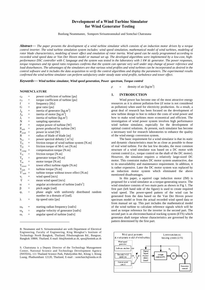
In this paper, a squirrel cage induction motor (IM) is proposed for a wind simulator as a torque-generating source. The wind simulator consists of two main parts as shown in Fig 1. The first part (left hand side of the figure) is used to create required wind speed. The power-speed pattern of the wind can be generated from the data based on the Van Der Hoven power spectrum model or from the actual recorded wind speed data or from manual set up. This part includes the mathematical model of the wind turbine to calculate reference signals which will be used as torque reference for the inverter in the second part. The second part is an electromechanical tracking system (ETS) which generates shaft torque whose characteristics are governed by the pattern determined by the first part.
Bunlung Neammanee, Somporn Sirisumrannukul and Somchai Chatratana
Development of a Wind Turbine Simulator for Wind Generator Testing
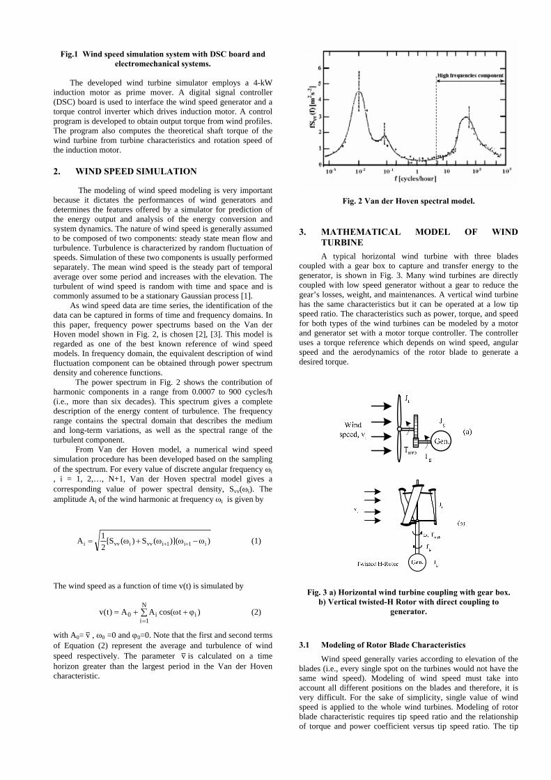
Fig.1 Wind speed simulation system with DSC board and
electromechanical systems.
The developed wind turbine simulator employs a 4-kW induction motor as prime mover. A digital signal controller (DSC) board is used to interface the wind speed generator and a torque control inverter which drives induction motor. A control program is developed to obtain output torque from wind profiles. The program also computes the theoretical shaft torque of the wind turbine from turbine characteristics and rotation speed of the induction motor.
2. WIND SPEED SIMULATION
The modeling of wind speed modeling is very important because it dictates the performances of wind generators and determines the features offered by a simulator for prediction of the energy output and analysis of the energy conversion and system dynamics. The nature of wind speed is generally assumed to be composed of two components: steady state mean flow and turbulence. Turbulence is characterized by random fluctuation of speeds. Simulation of these two components is usually performed separately. The mean wind speed is the steady part of temporal average over some period and increases with the elevation. The turbulent of wind speed is random with time and space and is commonly assumed to be a stationary Gaussian process [1].
As wind speed data are time series, the identification of the data can be captured in forms of time and frequency domains. In this paper, frequency power spectrums based on the Van der Hoven model shown in Fig. 2, is chosen [2], [3]. This model is regarded as one of the best known reference of wind speed models. In frequency domain, the equivalent description of wind fluctuation component can be obtained through power spectrum density and coherence functions.
The power spectrum in Fig. 2 shows the contribution of harmonic components in a range from 0.0007 to 900 cycles/h (i.e., more than six decades). This spectrum gives a complete description of the energy content of turbulence. The frequency range contains the spectral domain that describes the medium and long-term variations, as well as the spectral range of the turbulent component.
From Van der Hoven model, a numerical wind speed simulation procedure has been developed based on the sampling of the spectrum. For every value of discrete angular frequency ωi , i = 1, 2,…, N+1, Van der Hoven spectral model gives a corresponding value of power spectral density, Svv(ωi). The amplitude Ai of the wind harmonic at frequency ωi is given by
))]((S)(S[21A i1i1ivvivvi ω−ωω+ω= ++ (1)
The wind speed as a function of time v(t) is simulated by
)tcos(AA)t(v iN
1ii0 ϕ+ω+= ∑
= (2)
with A0= v , ω0 =0 and ϕ0=0. Note that the first and second terms of Equation (2) represent the average and turbulence of wind speed respectively. The parameter v is calculated on a time horizon greater than the largest period in the Van der Hoven characteristic.
Fig. 2 Van der Hoven spectral model.
3. MATHEMATICAL MODEL OF WIND TURBINE
A typical horizontal wind turbine with three blades coupled with a gear box to capture and transfer energy to the generator, is shown in Fig. 3. Many wind turbines are directly coupled with low speed generator without a gear to reduce the gear’s losses, weight, and maintenances. A vertical wind turbine has the same characteristics but it can be operated at a low tip speed ratio. The characteristics such as power, torque, and speed for both types of the wind turbines can be modeled by a motor and generator set with a motor torque controller. The controller uses a torque reference which depends on wind speed, angular speed and the aerodynamics of the rotor blade to generate a desired torque.
Fig. 3 a) Horizontal wind turbine coupling with gear box. b) Vertical twisted-H Rotor with direct coupling to
generator.
3.1 Modeling of Rotor Blade Characteristics
Wind speed generally varies according to elevation of the blades (i.e., every single spot on the turbines would not have the same wind speed). Modeling of wind speed must take into account all different positions on the blades and therefore, it is very difficult. For the sake of simplicity, single value of wind speed is applied to the whole wind turbines. Modeling of rotor blade characteristic requires tip speed ratio and the relationship of torque and power coefficient versus tip speed ratio. The tip
speed ratio (TSR), λ is obtained from
t
t
vRω
=λ (3)
The power captured by the blades, Pturb, can be calculated
using
),(cvR2
P P3t
2turb βλπ
ρ= (4)
The aerodynamic torque acting on the blades, Τturb, is
obtained by
),(cvR2
T T2t
3turb βλπ
ρ= (5)
If cP is known, the aerodynamic torque can also be calculated from
tP3t
2turb /),(cvR
2T ωβλπ
ρ= (6)
It can be seen from the above two equations that cT and cP
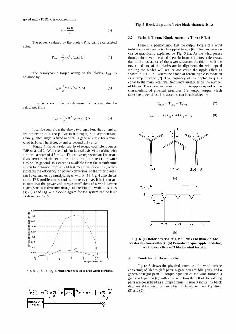
are a function of λ and β. But in this paper, β is kept constant; namely, pitch angle is fixed and this is generally true for a small wind turbine. Therefore, cT and cP depend only on λ. Figure 4 shows a relationship of torque coefficient versus TSR of a real 3 kW, three blade horizontal axis wind turbine with a rotor diameter of 4.5 m [4]. This curve represents an important characteristic which determines the starting torque of the wind turbine. In general, this curve is available from the manufacture or can be obtained from a field test. With this curve, cP , which indicates the efficiency of power conversion of the rotor blades, can be calculated by multiplying cT with λ [5]. Fig. 4 also shows the cP-TSR profile corresponding to the cP curve. It is important to note that the power and torque coefficient of a wind turbine depends on aerodynamic design of the blades. With Equations (3) - (5) and Fig. 4, a block diagram for the system can be built as shown in Fig. 5.
0 2 4 6 8 10 120
0.05
0.1
0.15
0.2
0.25
0.3
0.35
0.4
0.45
tip speed ratio
pow
er a
nd to
rque
coe
ffic
ient
[cP,
cT
]
cP
cT
[λ]
Fig. 4 cT-λ and cP-λ characteristic of a real wind turbine.
Fig. 5 Block diagram of rotor blade characteristics.
3.2 Periodic Torque Ripple caused by Tower Effect
There is a phenomenon that the output torque of a wind turbine contains periodically rippled torque [6]. The phenomenon can be graphically explained by Fig. 6 (a). As the wind passes through the tower, the wind speed in front of the tower decreases due to the resistance of the tower structure. At this time, if the tower and one of the blades are in alignment, the wind speed striking the blades will reduce and cause the ripple effect as shown in Fig 6 (b), where the shape of torque ripple is modeled as a ramp function [7]. The frequency of the rippled torque is equal to the main rotational frequency multiplies by the number of blades. The shape and amount of torque ripple depend on the characteristic of physical structures. Net output torque which takes the tower effect into account, can be calculated by
towerturbturb TTT −′= (7)
1fggtturb TGT)GJJ(T ++α+= (8)
(a)
(b)
Fig. 6 (a) Rotor position at 0, π /3, 2π/3 rad (black blade creates the tower effect). (b) Periodic torque ripple modeling
with tower effect of 3 blades wind turbine.
3.3 Emulation of Rotor Inertia
Figure 7 shows the physical structure of a wind turbine consisting of blades (left part), a gear box (middle part), and a generator (right part). A torque equation of the wind turbine is given in Equation (8) with an assumption that all of the rotating parts are considered as a lumped mass. Figure 8 shows the block diagram of the wind turbine, which is developed from Equations (3) and (8).
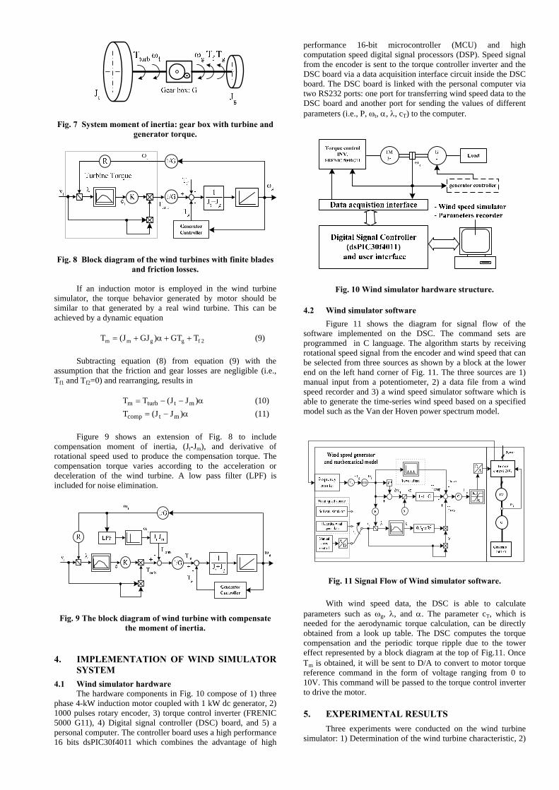
Fig. 7 System moment of inertia: gear box with turbine and generator torque.
Fig. 8 Block diagram of the wind turbines with finite blades
and friction losses.
If an induction motor is employed in the wind turbine simulator, the torque behavior generated by motor should be similar to that generated by a real wind turbine. This can be achieved by a dynamic equation
2fggmm TGT)GJJ(T ++α+= (9) Subtracting equation (8) from equation (9) with the
assumption that the friction and gear losses are negligible (i.e., Tf1 and Tf2=0) and rearranging, results in
α−−= )JJ(TT mtturbm (10)
α−= )JJ(T mtcomp (11) Figure 9 shows an extension of Fig. 8 to include
compensation moment of inertia, (Jt-Jm), and derivative of rotational speed used to produce the compensation torque. The compensation torque varies according to the acceleration or deceleration of the wind turbine. A low pass filter (LPF) is included for noise elimination.
Fig. 9 The block diagram of wind turbine with compensate the moment of inertia.
4. IMPLEMENTATION OF WIND SIMULATOR SYSTEM
4.1 Wind simulator hardware The hardware components in Fig. 10 compose of 1) three
phase 4-kW induction motor coupled with 1 kW dc generator, 2) 1000 pulses rotary encoder, 3) torque control inverter (FRENIC 5000 G11), 4) Digital signal controller (DSC) board, and 5) a personal computer. The controller board uses a high performance 16 bits dsPIC30f4011 which combines the advantage of high
performance 16-bit microcontroller (MCU) and high computation speed digital signal processors (DSP). Speed signal from the encoder is sent to the torque controller inverter and the DSC board via a data acquisition interface circuit inside the DSC board. The DSC board is linked with the personal computer via two RS232 ports: one port for transferring wind speed data to the DSC board and another port for sending the values of different parameters (i.e., P, ωt, α, λ, cT) to the computer.
Fig. 10 Wind simulator hardware structure.
4.2 Wind simulator software Figure 11 shows the diagram for signal flow of the
software implemented on the DSC. The command sets are programmed in C language. The algorithm starts by receiving rotational speed signal from the encoder and wind speed that can be selected from three sources as shown by a block at the lower end on the left hand corner of Fig. 11. The three sources are 1) manual input from a potentiometer, 2) a data file from a wind speed recorder and 3) a wind speed simulator software which is able to generate the time-series wind speed based on a specified model such as the Van der Hoven power spectrum model.
Fig. 11 Signal Flow of Wind simulator software.
With wind speed data, the DSC is able to calculate parameters such as ωg, λ, and α. The parameter cT, which is needed for the aerodynamic torque calculation, can be directly obtained from a look up table. The DSC computes the torque compensation and the periodic torque ripple due to the tower effect represented by a block diagram at the top of Fig.11. Once Τm is obtained, it will be sent to D/A to convert to motor torque reference command in the form of voltage ranging from 0 to 10V. This command will be passed to the torque control inverter to drive the motor.
5. EXPERIMENTAL RESULTS Three experiments were conducted on the wind turbine simulator: 1) Determination of the wind turbine characteristic, 2)
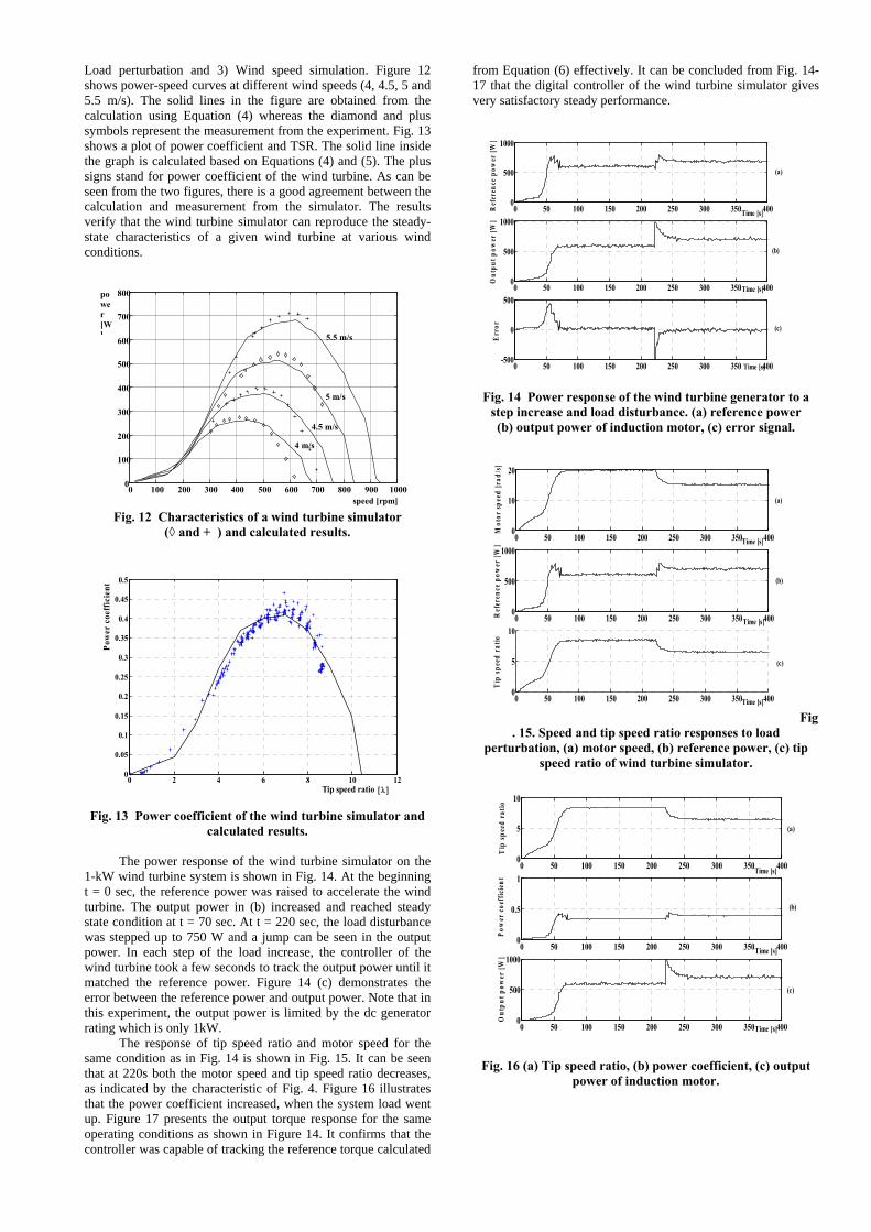
Load perturbation and 3) Wind speed simulation. Figure 12 shows power-speed curves at different wind speeds (4, 4.5, 5 and 5.5 m/s). The solid lines in the figure are obtained from the calculation using Equation (4) whereas the diamond and plus symbols represent the measurement from the experiment. Fig. 13 shows a plot of power coefficient and TSR. The solid line inside the graph is calculated based on Equations (4) and (5). The plus signs stand for power coefficient of the wind turbine. As can be seen from the two figures, there is a good agreement between the calculation and measurement from the simulator. The results verify that the wind turbine simulator can reproduce the steady-state characteristics of a given wind turbine at various wind conditions.
0 100 200 300 400 500 600 700 800 900 10000
100
200
300
400
500
600
700
800
speed [rpm]
power[W] 5.5 m/s
4 m/s
4.5 m/s
5 m/s
Fig. 12 Characteristics of a wind turbine simulator
(◊ and + ) and calculated results.
0 2 4 6 8 10 120
0.05
0.1
0.15
0.2
0.25
0.3
0.35
0.4
0.45
0.5
Tip speed ratio
Pow
er c
oeff
icie
nt
[λ] Fig. 13 Power coefficient of the wind turbine simulator and
calculated results.
The power response of the wind turbine simulator on the 1-kW wind turbine system is shown in Fig. 14. At the beginning t = 0 sec, the reference power was raised to accelerate the wind turbine. The output power in (b) increased and reached steady state condition at t = 70 sec. At t = 220 sec, the load disturbance was stepped up to 750 W and a jump can be seen in the output power. In each step of the load increase, the controller of the wind turbine took a few seconds to track the output power until it matched the reference power. Figure 14 (c) demonstrates the error between the reference power and output power. Note that in this experiment, the output power is limited by the dc generator rating which is only 1kW.
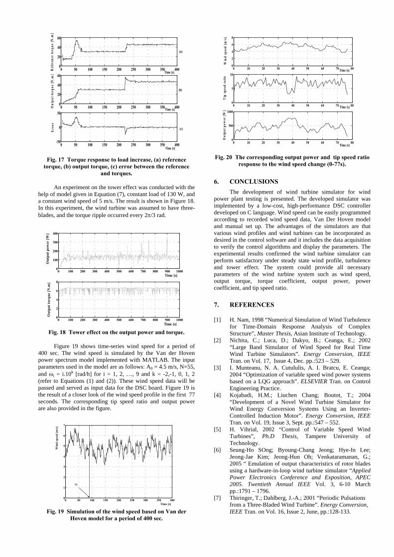
The response of tip speed ratio and motor speed for the same condition as in Fig. 14 is shown in Fig. 15. It can be seen that at 220s both the motor speed and tip speed ratio decreases, as indicated by the characteristic of Fig. 4. Figure 16 illustrates that the power coefficient increased, when the system load went up. Figure 17 presents the output torque response for the same operating conditions as shown in Figure 14. It confirms that the controller was capable of tracking the reference torque calculated
from Equation (6) effectively. It can be concluded from Fig. 14-17 that the digital controller of the wind turbine simulator gives very satisfactory steady performance.
0 50 100 150 200 250 300 350 4000
500
1000
Ref
eren
ce p
ower
[W]
Time [s]
0 50 100 150 200 250 300 350 4000
500
1000
Out
put p
ower
[W]
0 50 100 150 200 250 300 350 400-500
0
500
Err
or
Time [s]
Time [s]
(a)
(c)
(b)
Fig. 14 Power response of the wind turbine generator to a
step increase and load disturbance. (a) reference power (b) output power of induction motor, (c) error signal.
0 50 100 150 200 250 300 350 4000
10
20
Mot
or sp
eed
[rad
/s]
Time [s]
0 50 100 150 200 250 300 350 4000
500
1000
Ref
eren
ce p
ower
[W]
0 50 100 150 200 250 300 350 4000
5
10
Tip
spee
d ra
tio
Time [s]
Time [s]
(c)
(a)
(b)
Fig. 15. Speed and tip speed ratio responses to load
perturbation, (a) motor speed, (b) reference power, (c) tip speed ratio of wind turbine simulator.
0 50 100 150 200 250 300 350 4000
5
10
Tip
spee
d ra
tio
Time [s]
0 50 100 150 200 250 300 350 4000
0.5
1
Pow
er c
oeffi
cien
t
0 50 100 150 200 250 300 350 4000
500
1000
Out
put p
ower
[W]
Time [s]
Time [s]
(b)
(a)
(c)
Fig. 16 (a) Tip speed ratio, (b) power coefficient, (c) output
power of induction motor.
0 50 100 150 200 250 300 350 4000
20
40
60
Ref
eren
ce to
rque
[N.m
]
Time [s]
0 50 100 150 200 250 300 350 4000
20
40
60
Out
put t
orqu
e [N
.m]
0 50 100 150 200 250 300 350 400-50
0
50
Err
or
Time [s]
Time [s]
(a)
(c)
(b)
Fig. 17 Torque response to load increase, (a) reference
torque, (b) output torque, (c) error between the reference and torques.
An experiment on the tower effect was conducted with the
help of model given in Equation (7), constant load of 130 W, and a constant wind speed of 5 m/s. The result is shown in Figure 18. In this experiment, the wind turbine was assumed to have three-blades, and the torque ripple occurred every 2π/3 rad.
0 100 200 300 400 500 600 700 800 900 10000
100
200
300
400
Out
put p
ower
[W]
Time [s]
0 100 200 300 400 500 600 700 800 900 10000
2
4
6
8
Out
put t
orqu
e [N
.m]
Time [s] Fig. 18 Tower effect on the output power and torque.
Figure 19 shows time-series wind speed for a period of
400 sec. The wind speed is simulated by the Van der Hoven power spectrum model implemented with MATLAB. The input parameters used in the model are as follows: A0 = 4.5 m/s, N=55, and ωi = i.10k [rad/h] for i = 1, 2, …, 9 and k = -2,-1, 0, 1, 2 (refer to Equations (1) and (2)). These wind speed data will be passed and served as input data for the DSC board. Figure 19 is the result of a closer look of the wind speed profile in the first 77 seconds. The corresponding tip speed ratio and output power are also provided in the figure.
0 50 100 150 200 250 300 350 4000
1
2
3
4
5
6
7
Win
d sp
eed
[m/s
]
Time [s]
77
Fig. 19 Simulation of the wind speed based on Van der
Hoven model for a period of 400 sec.
0 10 20 30 40 50 60 70 800
2
4
6
8
Win
d sp
eed
[m/s]
Time [s]
0 10 20 30 40 50 60 70 800
5
10
Tip
spee
d ra
tio
Time [s]
0 10 20 30 40 50 60 70 800
500
1000
Out
put p
ower
[W]
Time [s]
Fig. 20 The corresponding output power and tip speed ratio
response to the wind speed change (0-77s).
6. CONCLUSIONS The development of wind turbine simulator for wind power plant testing is presented. The developed simulator was implemented by a low-cost, high-performance DSC controller developed on C language. Wind speed can be easily programmed according to recorded wind speed data, Van Der Hoven model and manual set up. The advantages of the simulators are that various wind profiles and wind turbines can be incorporated as desired in the control software and it includes the data acquisition to verify the control algorithms and display the parameters. The experimental results confirmed the wind turbine simulator can perform satisfactory under steady state wind profile, turbulence and tower effect. The system could provide all necessary parameters of the wind turbine system such as wind speed, output torque, torque coefficient, output power, power coefficient, and tip speed ratio.
7. REFERENCES
[1] H. Nam, 1998 “Numerical Simulation of Wind Turbulence for Time-Domain Response Analysis of Complex Structure”, Master Thesis, Asian Institute of Technology.
[2] Nichita, C.; Luca, D.; Dakyo, B.; Ceanga, E.; 2002 “Large Band Simulator of Wind Speed for Real Time Wind Turbine Simulators”. Energy Conversion, IEEE Tran. on Vol. 17, Issue 4, Dec. pp.:523 – 529. [3] I. Munteanu, N. A. Cutululis, A. I. Bratcu, E. Ceanga; 2004 “Optimization of variable speed wind power systems based on a LQG approach”. ELSEVIER Tran. on Control Engineering Practice. [4] Kojabadi, H.M.; Liuchen Chang; Boutot, T.; 2004 “Development of a Novel Wind Turbine Simulator for Wind Energy Conversion Systems Using an Inverter- Controlled Induction Motor”. Energy Conversion, IEEE Tran. on Vol. 19, Issue 3, Sept. pp.:547 – 552. [5] H. Vihrial, 2002 “Control of Variable Speed Wind Turbines”, Ph.D Thesis, Tampere University of Technology. [6] Seung-Ho SOng; Byoung-Chang Jeong; Hye-In Lee; Jeong-Jae Kim; Jeong-Hun Oh; Venkataramanan, G.; 2005 “ Emulation of output characteristics of rotor blades using a hardware-in-loop wind turbine simulator “Applied Power Electronics Conference and Exposition, APEC 2005. Twentieth Annual IEEE Vol. 3, 6-10 March pp.:1791 – 1796. [7] Thiringer, T.; Dahlberg, J.-A.; 2001 “Periodic Pulsations from a Three-Bladed Wind Turbine”. Energy Conversion, IEEE Tran. on Vol. 16, Issue 2, June, pp.:128-133.


![Velocity Adjustable Wind Turbine Simulator based onActual Wind ... · Neammanee. B et al.[7] presented a wind turbine simulator which uses induction motor driven by the invertor to](https://img.pdfslide.net/doc/110x75/5f2f32866cfaa12ef5634df3/velocity-adjustable-wind-turbine-simulator-based-onactual-wind-neammanee-b.jpg)