Embed Size (px)
Citation preview
Copyright 2003, Elsevier Science (USA)
This book is printed on acid-free paper. @
All rights reserved.
No part of this publication may be reproduced or transmitted in any form or by anymeans, electronic or mechanical, including photocopy, recording, or any informationstorage and retrieval system, without permission in writing from the publisher.
Permissions may be sought directly from Elsevier's Science ts: Technology RightsDepartment in Oxford, UK: phone: (+44) 1865843830, fax: (+44) 1865853333, e-mail:[email protected]. You may also complete your request on-line via the ElsevierScience homepage (http://elsevier.com),by selecting "Customer Support" and then"Obtaining Perrnissions."
Academic PressAn imprint of Elsevier Science525 B Street, Suite 1900, San Diego, California 92101-4495, USAhttp://www.academicpress.com
Academic PressAn imprint of Elsevier Science84 Theobald's Road, London WC1X 8RR, UKhttp://www.academicpress.com
Academic PressAn imprint of Elsevier Science200 Wheeler Road, Burlington, Massachusetts 01803, USAwww.academicpressbooks.com
Library of Congress Catalog Card Number: 2002117166
International Standard Book Number: 0-12-141360-8
PRINTED IN THE UNITED STATES OF AMERICAO 3 04 05 06 9 8 7 6 5 4 3 2 1
2/Decision Methods for Forest Resource Management ©2003 Joseph Buongiorno and Keith Gilless
1
Chapter 2 __________________________________________________________________
Principles of Linear Programming: Formulations
2.1 INTRODUCTION
This chapter is an introduction to the method of linear programming. Here we shall deal mostly with simple examples showing how a management problem can be formulated as a special mathematical model called a linear program. We shall concentrate on formulation, leaving the question of how to solve linear programs to the next chapter.
Linear programming is a very general optimization technique. It can be applied to many different problems, some of which have nothing to do with forestry or even management science. Nevertheless, linear programming was designed and is used primarily to solve managerial problems. In fact, it was one of the first practical tools to tackle complex decision-making problems common to industry, agriculture, and government.
For our immediate purpose, linear programming can be defined as a method to allocate limited resources to competing activities in an optimal manner.
This definition describes well the situation faced by forest managers. The resources with which they work, be they land, people, trees, time or money, are always limited. Furthermore, many of the activities that managers administer compete for these resources. For example, one may want to increase the land area that is growing red pine, but then less land will be available for aspen. Another may want to assign more of her staff to prepare timber sales, but then fewer people will be available to do stand improvement work. She could hire more people, but then she would have too little money.
No matter what course of action they choose managers always face constraints that limit the range of their options. Linear programming is designed to help them choose. Not only can the method show which alternatives are possible (“feasible” in linear programming jargon), it can also help determine the best one. But this requires that both the management objective as well as the constraints be defined in a precise mathematical manner. Finding the best
2/Decision Methods for Forest Resource Management ©2003 Joseph Buongiorno and Keith Gilless
2
alternative is a recurring theme in management science and most of the methods presented in this book involve optimization models.
The first practical way of solving linear programs, the simplex method, was invented by George Dantzig in the late nineteen forties. At first, by hand and with mechanical desk calculators, only small problems could be solved. Using computers and linear programming, one can now routinely solve problems with several thousands of variables and constraints.
Linear programming is by far the most widely used operations research method. Although simulation (which we shall examine in Chaps. 14 and 15) is also a very effective method, linear programming has been and continues to be used intensively in forest management. Some of the most widely used forest planning models to date, in the United States and abroad, in industry and on National Forests, use linear programming or its close cousin, goal programming, which we shall study in Chap. 10.
2.2 FIRST EXAMPLE: A POET AND HIS WOODS
This first example of application of linear programming is certainly artificial, too simple to correspond to a real forestry operation. Nevertheless, it will suffice to introduce the main concepts and definitions. Later on we will use this same example to discuss the graphical and simplex methods of solving linear program.
Anyway, the story is romantic.
Problem Definition
The protagonist is a congenial poet-forester who lives in the woods of Northern Wisconsin. Some success in his writing allowed him to buy, about ten years ago, a cabin and 90 ha of woods in good productive condition.
The poet needs to walk the beautiful woods to keep his inspiration alive. But the muses do not always respond and he finds that sales from the woods come very handy to replenish a sometimes empty wallet. In fact, times have been somewhat harder than usual lately. He has firmly decided to get the most he can out of his woods.
But the arts must go on. The poet does not want to spend more than half of his time in the woods; the rest is for prose and sonnets.
Our poet has a curious mind. He has even read about linear programming: A method to allocate scarce resources to optimize certain objectives. He thinks that this is exactly what he needs to get the most out of his woods, while pursuing his poetic vocation.
2/Decision Methods for Forest Resource Management ©2003 Joseph Buongiorno and Keith Gilless
3
Data
In order to develop his model the poet has put together the following information:
About 40 ha of the land he owns are covered with red-pine plantations. The other 50 ha contain mixed northern hardwoods. Having kept a very good record of his time, he figures that since he bought these woods he has spent approximately 800 days managing the red pine and 1500 days on the hardwoods. The total revenue from his forest during the same period was $36,000 from the red pine land and $60,000 from the northern hardwoods.
Problem formulation
Decision variables To formulate his model, the poet-forester needs to choose the variables to symbolize his decisions. The choice of proper decision variables is critical in building a model. Some choices will make the problem far simpler to formulate and solve than others. Unfortunately, there is no set method for choosing decision variables. It is part of the art of model building, which can only be learned by practice.
Nevertheless, the nature of the objective will often give some clue as to what the decision variables should be.
We noted above that the poet’s objective is to maximize his revenues from the property. But this has a meaning only if the revenues are finite; thus he must mean revenues per unit of time, say per year (meaning an average year, like anyone of the past ten enjoyable years that the poet has spent on his property). Formally, we begin to write the objective as:
Maximize Z = $ of revenues per year. The revenues symbolized by the letter Z arise from managing red pine, or
northern hardwoods, or both. Therefore, a natural set of decision variables is: X
1 = the number of hectares of red pine to manage
X2 = the number of hectares of northern hardwoods to manage
These are the unknowns. We seek the values of X
1 and X
2 that make Z as
large as possible.
2/Decision Methods for Forest Resource Management ©2003 Joseph Buongiorno and Keith Gilless
4
Objective Function The objective function expresses the relationship between Z, the revenues generated by the woods, and the decision variables X
1 and X
2. To
write this function, we need an estimate of the yearly revenues generated by each type of forest. Since the poet has earned $36,000 on 40 ha of red pine and $60,000 on 50 ha of northern hardwoods during the past 10 years, the average earnings have been $90 per ha per year (90 $/ha/y) for red pine, and 120 $/ha/y for northern hardwoods. Using these figures as measures of the poet's expected revenues during the coming years, we can now write his objective function as:
)ha(2
)y/ha/($)ha(1
)y/ha/($)y/($12090max XXZ +=
where the units of measurement of each variable and constant are shown in parentheses. A good modeling practice is to always check the homogeneity of all algebraic expressions with respect to the units of measurement. Here, Z is expressed in dollars per year; therefore, the operations on the right of the equal sign must also yield dollars per year, which they do.
To complete the model, we must determine what constraints limit the actions of our poet forester and then help him express these constraints in terms of the decision variables, X
1 and X2.
Land Constraints Two constraints are very simple. The area managed in each timber type cannot exceed the area available, that is:
401 ≤X ha of red pine
502 ≤X ha of northern hardwoods
Time Constraint Another constraint is set by the fact that the poet does not want to spend more than half his time, let us say 180 days a year, managing his woods. In order to write this constraint in terms of the decision variables, we note that the time he has spent managing red pine during the past 10 years (800 days for 40 ha of land) averages to 2 days per hectare per year (2 d/ha/y). Similarly, he has spent 3 d/ha/y on northern hardwoods (1500 days on 50 ha).
In terms of the decision variables X1 and X
2, the total time spent by the
poet-forester to manage his woods is:
)()(3
)()(2
ha
2
d/ha/yha
1
d/ha/y
XX +
and the expression of the constraint limiting this time to no more than 180 days is:
)d/y()ha(2
)d/ha/y()ha(1
)d/ha/y(18032 ≤+ XX
2/Decision Methods for Forest Resource Management ©2003 Joseph Buongiorno and Keith Gilless
5
Non Negativity Constraints The last constraints needed to complete the formulation of the problem state that none of the decision variables may be negative, since they refer to areas. Thus:
01 ≥X and 02 ≥X
Final Model In summary, combining the objective function and the constraints, we obtain the complete formulation of the poet-forester problem as: Find the variables X
1 and X
2, which measure the number of hectares of red-pine and of
northern hardwoods to manage, such that:
0,
18032
50
40
:subject to
12090max
21
21
2
1
21
≥
≤+
≤
≤
+=
XX
XX
X
X
XXZ
Note that northern hardwoods are cultivated under a selection system.
This requires more time per land area, especially to mark the trees to be cut, than the even-aged red pine. But in exchange, the hardwoods tend to return more per unit of land, as reflected in the objective function. Therefore, the choice of the best management strategy is not obvious.
In the next chapter we will learn how to solve this problem. But before that, let us consider another example.
2.3 SECOND EXAMPLE: KEEPING THE RIVER CLEAN
The purpose of this second example is to illustrate the formulation of a linear programming model that, in contrast to the poet's problem, involves minimizing an objective function, and constraints of the greater-than-or-equal-to form.
Also, in this problem, we move away from the strict interpretation of constraints as limits on available resources. Here, some of the constraints will express management objectives. Furthermore, this example shows that the objective function being optimized does not have to express monetary returns or costs. Indeed, because it is a general optimization method, linear programming has much broader applications than strictly financial ones.
2/Decision Methods for Forest Resource Management ©2003 Joseph Buongiorno and Keith Gilless
6
Problem Definition This story deals with a pulp mill operating in a small town in Maine. The
pulp mill makes mechanical and chemical pulp. Unfortunately, it also pollutes the river in which it spills its spent waters. This has created enough turmoil to change the management of the mill completely.
The previous owners felt that it would be too costly to reduce the pollution problem. They decided to sell. The mill has been bought back by the employees and local businesses, who now own the mill as a cooperative.
The new owners have several objectives. One is to keep at least 300 people employed at the mill. Another is to generate at least $40,000 of revenue per day. They estimate that this will be enough to pay operating expenses and yield a return that will keep the mill competitive in the long run. Within these limits, everything possible should be done to minimize pollution.
A bright forester who has already provided shrewd solutions to complex wood procurement problems is asked to suggest an operating strategy for the mill that will meet all these objectives simultaneously, and in the best possible way. She feels that it could be done by linear programming. Towards this end, she has put together the following data:
Both chemical and mechanical pulp require the labor of one worker for about 1 day, or 1 workday (wd), per ton produced.
The chemical pulp sells at some $ 200 per ton, the mechanical pulp at $100.
Pollution is measured by the biological oxygen demand (BOD). One ton of mechanical pulp produces 1 unit of BOD, one ton of chemical pulp produces 1.5 units.
The maximum capacity of the mill to make mechanical pulp is 300 tons per day; for chemical pulp it is 200 tons per day. The two manufacturing processes are independent; that is, the mechanical pulp line cannot be used to make chemical pulp, and vice versa.
Given this, our forester has found that the management objectives and the technical and financial data could be put together into a linear program. This is how she did it:
Linear Programming Formulation
Decision Variables Pollution, employment, and revenues, result from the production of both types of pulp. A natural choice for the decision variables is then:
X1 = amount of mechanical pulp produced (in tons per day, or t/d) and
X2 = amount of chemical pulp produced (t/d)
2/Decision Methods for Forest Resource Management ©2003 Joseph Buongiorno and Keith Gilless
7
Objective Function The objective function to minimize is the amount of pollution, Z, measured here by units of BOD per day. In terms of the decision variables, this is:
)t/d(2
)BOD/t()t/d(1
)BOD/t()BOD/d(5.11min XXZ +=
where the units of measurement are shown in parentheses. Verify that the objective function is homogeneous in units. That is, that the operations on the right-hand side of the equality sign give a result in BOD/d.
Employment Constraint One constraint expresses the objective to keep at least 300 workers employed. In terms of the decision variables, this is:
)workers()t/d(2
wd/t)()t/d(1
)wd/t(30011 ≥+ XX
Revenue Constraint A second constraint states that at least $40,000 of revenue must be generated every day:
)d/$()t/d(2
$/t)()t/d(1
)$/t(000,40200100 ≥+ XX
Capacity Constraints Two other constraints refer to the fact that the daily production capacity of the mill cannot be exceeded:
)/()/(1 300
dtdt
X ≤ (mechanical pulp)
)/()/(2 200
dtdt
X ≤ (chemical pulp)
Non Negativity Constraints The quantity of mechanical and chemical pulp produced must be positive or zero, that is:
01 ≥X and 02 ≥X
In summary, the final form of the linear program that models the dilemma
of the pulp-making cooperative is to find the values of X1 and X
2, which measure
the amount of mechanical and chemical pulp produced daily, such that:
2/Decision Methods for Forest Resource Management ©2003 Joseph Buongiorno and Keith Gilless
8
0,
200
300
000,40200100
300
:subject to
5.1min
21
2
1
21
21
21
≥
≤
≤
≥+
≥+
+=
XX
X
X
XX
XX
XXZ
A Note on Multiple Objectives In this example, although there were several management objectives (pollution, employment, and revenue), only one of them was expressed by the objective function. The other objectives were expressed as constraints. The fact that there is only one objective function is a general rule and not peculiar to linear programming. In any optimization problem, only one function can be optimized.
For example, strictly speaking, it makes no sense to say that we want to maximize the amount of timber that a forest produces AND maximize the recreation opportunities offered in the same forest. As long as timber and recreation conflict, that is as long as they use common resources, we must choose between two options: Either we maximize timber, subject to a specified amount of recreation opportunities, or we maximize recreation subject to a certain volume of timber production.
One of the teachings of linear programming is that we must choose which objective to optimize. Later, we will study methods designed to handle several objectives with more flexibility. Goal programming is one such method, but even in goal programming (as we shall see in Chap. 10), the optimized objective function is unique.
2.4 STANDARD FORMULATION OF A LINEAR PROGRAMMING PROBLEM
Any linear program may be written in several equivalent ways. For example, like the poet’s problem, the river pollution problem can be rewritten as a maximization subject to less-than-or-equal-to constraints, the so-called standard form, as follows:
2/Decision Methods for Forest Resource Management ©2003 Joseph Buongiorno and Keith Gilless
9
0,
200
300
000,40200100
300
:subject to
5.1)max(
21
2
1
21
21
21
≥
≤
≤
−≤−−
−≤−−
−−=−
XX
X
X
XX
XX
XXZ
the minimization of the objective function has been changed to a maximization of its opposite, and the direction of the first two inequalities has been reversed by multiplying both sides by –1.
Strict equality constraints can also be expressed as less-than-or-equal-to constraints. For example if the cooperative wanted to employ exactly 300 workers, the first constraint above would be:
30021 =+ XX
which is equivalent to the two inequalities:
30021 ≤+ XX and 30021 ≥+ XX
the second of which can be rewritten as a less-than-or-equal-to constraint:
30021 −≤−− XX
Furthermore, if any variable in a problem, say X3, might take a negative
value (for example if X3 designated the deviation with respect to a goal), then it could be replaced in the model by the difference between two non-negative variables:
543 XXX −= with 0 and 0 54 ≥≥ XX
Thus, a linear programming problem may have an objective function that is maximized or minimized, constraints may be inequalities in either direction or strict equalities, and variables may take positive or negative values. Still, the problem can always be recast in the equivalent standard form, with an objective function that is maximized, inequalities that are all of the less-than-or-equal-to type, and variables that are all non negative. The general expression of this standard form is:
2/Decision Methods for Forest Resource Management ©2003 Joseph Buongiorno and Keith Gilless
10
Find the values of n variables, X1, X
2,..., X
n (referred to as decision
variables, or activities) such that the objective function, Z, is maximized. The objective function is a linear function of the n decision variables:
XcXcXcZ n+++= ...max 2211
where c
1,..., c
n are all constant parameters. Each parameter, c
j, measures the
contribution of the corresponding variable Xj to the objective function. For
example, if X1 increases (decreases) by one unit, then, other variables remaining
equal, Z increases (decreases) by c1 units.
The values that the variables can take in trying to maximize the objective function are limited by m constraints. The constraints have the following general expression:
mnmnmm
nn
nn
bXaXaXa
bXaXaXa
bXaXaXa
≤+++
≤+++
≤+++
...
...
...
...
2211
22222121
11212111
Where b
1, b
2,...,b
m are constants. These constants often reflect the
amounts of available resources. For example, b1 could be the land area that a
manager can use, b2 the amount of money available to spend. In that case, each a
ij
is a constant that measures how much of resource i is used per unit of activity j. For example, keeping the interpretation of b
2 just given, and assuming that X
1 is
the number of hectares planted in a given year, a21
is the cost of planting one
hectare.
More generally, this interpretation means that the product jij Xa is the
amount of resource i used when activity j is at the level Xj . Adding these
products up over all activities leads to the following general expression for the total amount of resource i used by all n activities:
niniii XaXaXaR +++= ...2211 In linear programming R
i is referred to as the row activity i, in symmetry
with the column activity, Xj.
Adding the non negativity constraints completes the standard form:
0,...,, 21 ≥nXXX
2/Decision Methods for Forest Resource Management ©2003 Joseph Buongiorno and Keith Gilless
11
The standard linear programming model can be expressed in a more
compact form by using the Greek capital letter sigma (∑ ) to indicate
summations. The general linear programming problem is then to find Xj (j =1,..., n) such that:
njX
mibX
XcZ
j
n
j
ijij
n
j
jj
,...,1for 0
,...,1for a
:subject to
max
1
1
=≥
=≤
=
∑
∑
=
=
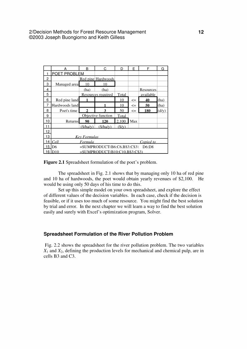
2.5 SPREADSHEET FORMULATION OF LINEAR PROGRAMS Much of the power of mathematical models stems from the ability to formulate and solve them quickly with computers. For ease of learning and application, modern spreadsheets have become the ideal software to handle many management models. Throughout this book, we shall give examples of modeling with the Excel software. Like several other spreadsheets, Excel contains a Solver to find the best solution of linear programs and other problems. Spreadsheet Formulation of the Poet’s Problem Fig. 2.1 shows how the poet’s problem can be formulated in a spreadsheet. All the fixed parameters, that is the data, are in bold characters, while the variables, or the cells that depend on the variables, are not. The decision variables, or activities, X1 and X2 are in cells B3:C3. The amounts of land and time available are in cells F6:F8. The data in the cells B6:C8 are the amounts of resources used per unit of each activity. The data in cells B10:C10 are the revenues per unit of each activity.
The cells D6:D8 contain formulas expressing the amount of resource used by the activities (the row activities). For example, the formula in cell D6 is the equivalent of 1X1 +0X2 expressing the amount of red pine managed by the poet. The “<=” symbols in cells E6:E8 remind us that the amounts of resources used should not exceed the amounts available.
The cell D10 contains the formula of the objective function, the equivalent of Z=90X1+120X2.
2/Decision Methods for Forest Resource Management ©2003 Joseph Buongiorno and Keith Gilless
12
Figure 2.1 Spreadsheet formulation of the poet’s problem.
The spreadsheet in Fig. 2.1 shows that by managing only 10 ha of red pine
and 10 ha of hardwoods, the poet would obtain yearly revenues of $2,100. He would be using only 50 days of his time to do this.
Set up this simple model on your own spreadsheet, and explore the effect of different values of the decision variables. In each case, check if the decision is feasible, or if it uses too much of some resource. You might find the best solution by trial and error. In the next chapter we will learn a way to find the best solution easily and surely with Excel’s optimization program, Solver.
Spreadsheet Formulation of the River Pollution Problem Fig. 2.2 shows the spreadsheet for the river pollution problem. The two variables X1 and X2, defining the production levels for mechanical and chemical pulp, are in cells B3 and C3.
1
2
3
4
5
6
7
8
9
10
11
12
13
14
15
16
A B C D E F G
POET PROBLEM
Red pine Hardwoods
Managed area 10 10
(ha) (ha) Resources
Total available
Red pine land 1 10 <= 40 (ha)
Hardwoods land 1 10 <= 50 (ha)
Poet's time 2 3 50 <= 180 (d/y)
Total
Returns 90 120 2,100 Max
($/ha/y) ($/ha/y) ($/y)
Key Formulas
Cell Formula Copied to
D6 =SUMPRODUCT(B6:C6,B$3:C$3) D6:D8
D10 =SUMPRODUCT(B10:C10,B$3:C$3)
Resources required
Objective function
2/Decision Methods for Forest Resource Management ©2003 Joseph Buongiorno and Keith Gilless
13
1
2
3
4
5
6
7
8
9
10
11
12
13
14
15
16
17
A B C D E F G
RIVER POLLUTION PROBLEM
Mech pulp Chem pulp
Production 100 100
(t/d) (t/d)
Total
Employment 1 1 200 >= 300 workers
Revenues 100 200 30000 >= 40000 $/d
Mech capacity 1 100 <= 300 t/d
Chem capacity 1 100 <= 200 t/d
Total
Pollution 1 1.5 250 Min
BOD/t BOD/t BOD/d
Key Formulas
Cell Formula Copied to
D6 =SUMPRODUCT(B6:C6,B$3:C$3) D6:D9
D11 =SUMPRODUCT(B11:C11,B$3:C$3)
Objective function
Constraints
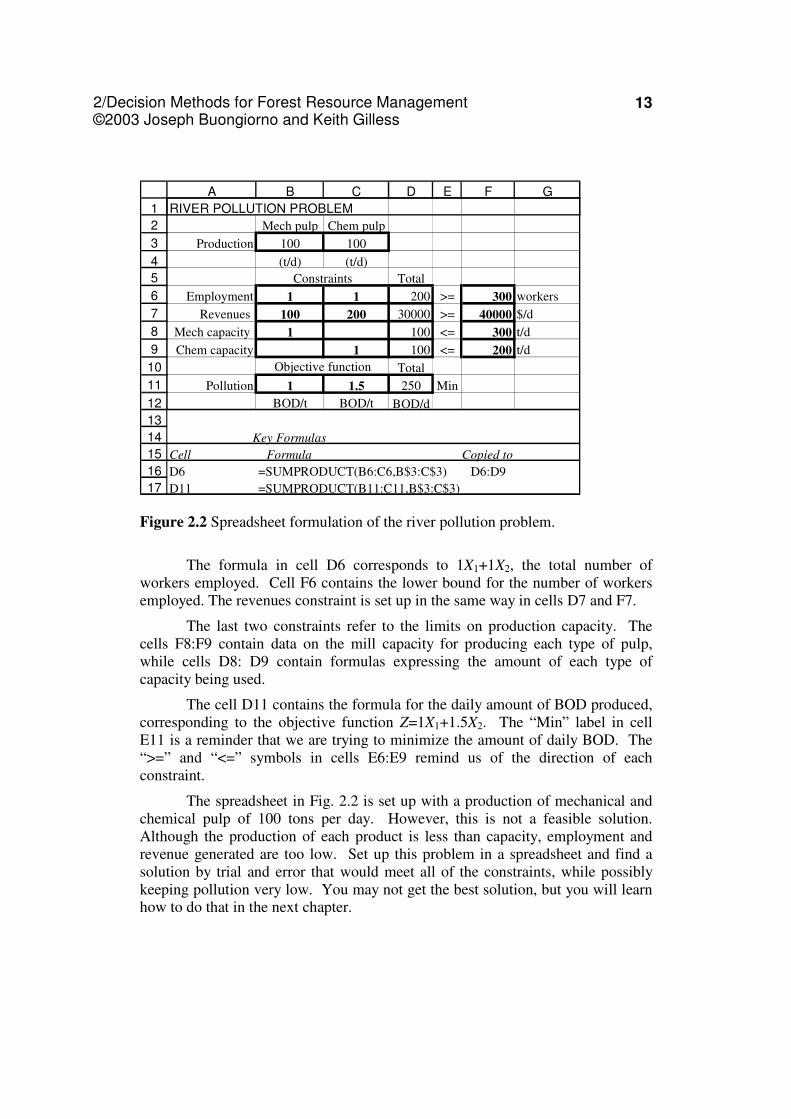
Figure 2.2 Spreadsheet formulation of the river pollution problem.
The formula in cell D6 corresponds to 1X1+1X2, the total number of workers employed. Cell F6 contains the lower bound for the number of workers employed. The revenues constraint is set up in the same way in cells D7 and F7.
The last two constraints refer to the limits on production capacity. The cells F8:F9 contain data on the mill capacity for producing each type of pulp, while cells D8: D9 contain formulas expressing the amount of each type of capacity being used.
The cell D11 contains the formula for the daily amount of BOD produced, corresponding to the objective function Z=1X1+1.5X2. The “Min” label in cell E11 is a reminder that we are trying to minimize the amount of daily BOD. The “>=” and “<=” symbols in cells E6:E9 remind us of the direction of each constraint.
The spreadsheet in Fig. 2.2 is set up with a production of mechanical and chemical pulp of 100 tons per day. However, this is not a feasible solution. Although the production of each product is less than capacity, employment and revenue generated are too low. Set up this problem in a spreadsheet and find a solution by trial and error that would meet all of the constraints, while possibly keeping pollution very low. You may not get the best solution, but you will learn how to do that in the next chapter.
2/Decision Methods for Forest Resource Management ©2003 Joseph Buongiorno and Keith Gilless
14
2.6 ASSUMPTIONS OF LINEAR PROGRAMMING
Before proceeding to study the solutions and applications of linear programming, it is worth stressing the assumptions that it makes. A linear programming model is a satisfactory representation of a particular management problem when all these assumptions are warranted. They will never hold exactly, but they should be reasonable. The determination of what is reasonable or not is part of the art of management and model building. Keep in mind that bold assumptions are more useful in understanding the world than complicated details.
Proportionality
A linear programming model assumes that the contribution of any activity to the objective function is directly proportional to the level of that activity. As the level of the activity increases or decreases, the change in the objective function due to a unit change of the activity remains the same. For example, in the poet-forester problem, the contribution of red pine management to revenues is directly proportional to the area of red pine being managed.
In a similar manner, the amount of resource used by each activity is assumed to be directly proportional to the level of that activity. For example, the time the poet must put managing his land is directly proportional to the area being managed. If, as the managed area increased, each additional hectare required an increasing amount of time, then the linear programming model would not be valid, at least not without some modification.
Additivity
A linear programming model assumes that the contribution of all activities to the objective function is just the sum of the contributions of each activity considered independently. Similarly, the total amount of a resource used by all activities is assumed to be the sum of the amounts used by each individual activity considered independently. This means that the contribution of each variable does not depend on the presence or absence of the others.
In our example, regardless of what the poet-forester does with his northern hardwoods, he will always get $90 per hectare from each hectare of managed red pine, and it will still take him 2 days per hectare per year to manage.
2/Decision Methods for Forest Resource Management ©2003 Joseph Buongiorno and Keith Gilless
15
Divisibility
A linear programming model assumes that all activities are continuous and can take any positive value. This means that linear programming models are not generally suitable in situations where the decision variables can take only integer values. For example, management decisions may require yes or no answers: Should we build this bridge or not?
For some problems that involve integer variables, it may be enough to compute a continuous solution by ordinary linear programming and then round the variables to the nearest integer. But this is not always appropriate. We will study programming models that use integer variables in Chap. 11.
Determinism
A linear programming model is deterministic. In computing a solution, it does not take into account that all of the coefficients in the model are only approximations.
For this reason, it is wise when using linear programming to compute not only one solution, but several. Each solution corresponds to different, but reasonable, assumptions regarding the values of the parameters. Such sensitivity
analysis shows how sensitive a solution is to changes in the values of parameters. In order to arrive at good decisions, one should examine carefully those parameters that have the most impact.
Most of the models examined in this book are deterministic. Stochastic models, in which the random nature of some parameters is considered explicitly, will be examined in Chaps. 12 and 13 on network analysis and dynamic programming, in Chaps. 14 and 15 on simulation, and in Chaps. 16 and 17 on Markov chains. Interestingly, the linear programming method will turn out to be useful even to solve some stochastic problems.
2.7 CONCLUSION
The two examples considered in this chapter have shown the flexibility of linear programming. Problems involving the optimization of a specific objective, subject to constraints can be cast as linear programs. The objective may be to minimize or maximize something. The constraints may represent the limited resources that the manager can work with, but they may also refer to objectives. Only one objective can be optimized.
Formulating a forest management problem so that it could be solved by linear programming is not always easy. It takes ingenuity and much practice, plus some courage. To be understood, the world must be simplified, this is what models are all about. Linear programming is not different: it makes some drastic
2/Decision Methods for Forest Resource Management ©2003 Joseph Buongiorno and Keith Gilless
16
assumptions. But the assumptions are not so critical as to render the method useless. On the contrary, we shall discover in the forthcoming chapters that linear programming is so flexible that it can be usefully applied to a wide array of forest management problems, from harvest scheduling and multiple-use planning to investment analysis. It can even help deal with uncertainty. There is almost no limit, except our imagination.
PROBLEMS
2.1. Several management problems are listed below. What kind of objective function would
be appropriate in a linear programming model for each? What kinds of decision variables? What kinds of constraints? (a) A farmer wants to maximize the income he will receive over the next twenty years
from his woodlot. The woodlot is covered with mature sugar maple trees that could be sold as stumpage or managed to produce maple syrup.
(b) The manager of a hardwood sawmill wants to maximize the mill's net revenues. The mill can produce pallet stock, dimension lumber, or some combination of the two. Pallet stock commands a lower price than dimension lumber, but it can be produced from less expensive logs, and the daily capacity of the mill to produce pallet stock exceeds its capacity to produce dimension lumber.
(c) A logging contractor wants to minimize the cost of harvesting a stand of timber. She can use mechanical fellers, workers with chainsaws, or some of both. Leasing and operating a mechanical feller is more expensive than hiring a worker with a chainsaw, but it can do more work per hour. On the other hand, a mechanical feller cannot be used to harvest some of the largest and most valuable trees in the stand.
2.2. Consider the linear programming model of the poet and his woods in Sec. 2.2.
(a) If the poet had received $50,000 over the last ten years from managing his red pine plantations and $30,000 from managing his hardwoods, how would the coefficients of X
1 and X
2 change in the objective function?
(b) Suppose that the poet found that time spent pruning branches had a particularly inhibiting effect on his literary endeavors, and that two thirds of the time devoted to managing hardwoods had to be spent pruning. If he wanted to limit the time he spent pruning to not more than 70 days per year, what constraint would have to be added to the model?
(c) If one half of the time devoted to managing red pine plantations had to be spent pruning, how would this constraint have to be further modified?
2.3. Consider the linear programming model of pulp mill management in Sec. 2.3. The mill management might prefer to maximize gross revenues while limiting pollution to not more than 300 BOD per day. Reformulate the model to reflect this new management orientation, leaving the employment and capacity constraints unchanged.
2.4. Consider the linear programming model of the poet and his woods in Sec. 2.2.
2/Decision Methods for Forest Resource Management ©2003 Joseph Buongiorno and Keith Gilless
17
(a) If the poet decided to manage 25 acres of red pine and 35 acres of hardwoods, how much income would he receive from his lands each year?
(b) How much of his time would he need to manage his lands? 2.5. Consider the linear programming model of pulp mill management in Sec. 2.3.
(a) If the mill's management decided to produce 150 tons of chemical pulp and 190 tons of mechanical pulp per day, how much pollution would result?
(b) How much revenue would this decision generate? (c) How many people would be employed?
2.6. A logging contractor wants to maximize net revenues per day from the operation of her
four tractor-skidders and six wheeled-skidders. From her records, she estimates that her net revenue per day of operation for a tractor at $300, and for a skidder at $600. Only eighteen people trained to operate this kind of logging equipment are available in the local labor market, and it takes two people to run a skidder and three to run a tractor. (a) Formulate this problem as a linear program, defining the units of all decision
variables, coefficients, and parameters in the model. (b) What logical constraints must be placed on the values may each decision variable
can take? (c) Can this problem be solved as an ordinary linear program?
2.7. A logging contractor wants to allocate her logging equipment between two logging sites
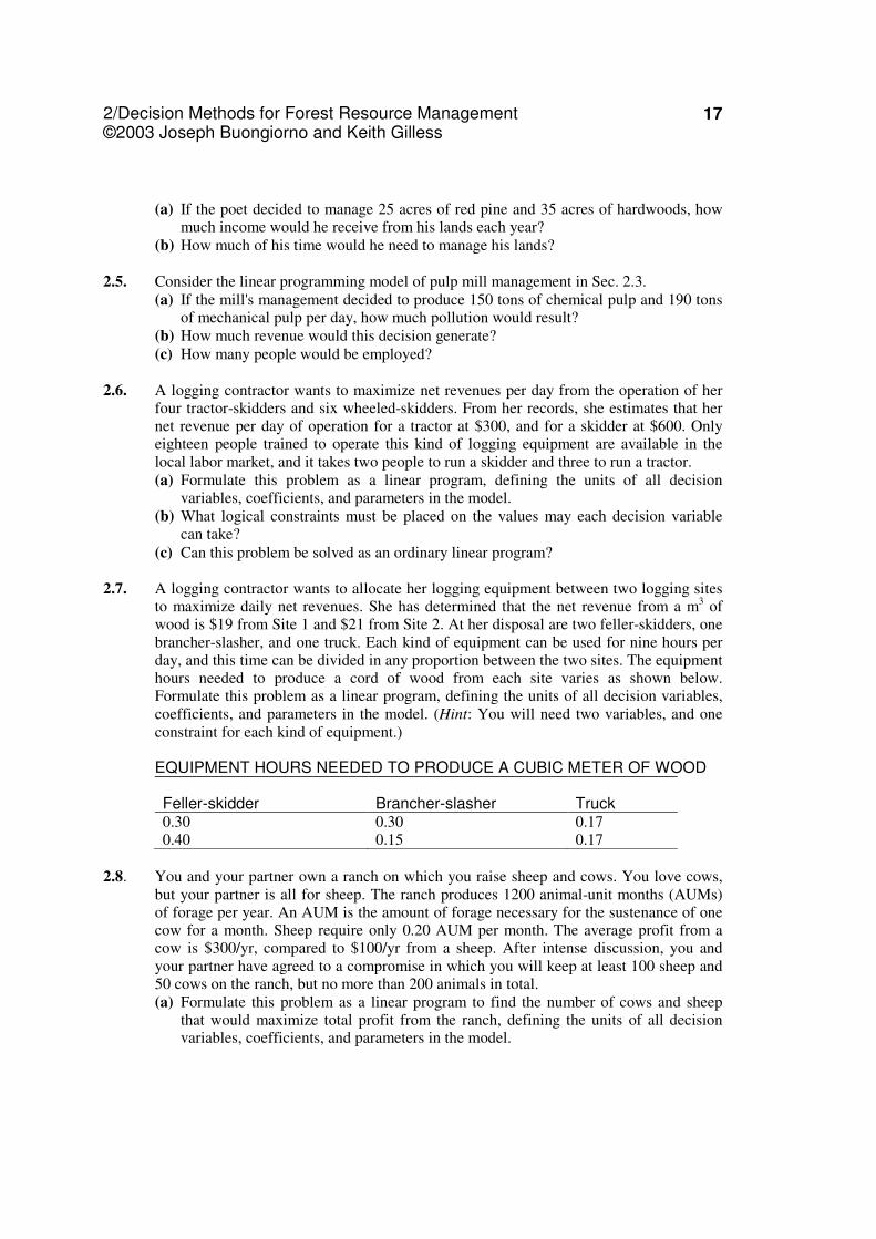
to maximize daily net revenues. She has determined that the net revenue from a m3 of wood is $19 from Site 1 and $21 from Site 2. At her disposal are two feller-skidders, one brancher-slasher, and one truck. Each kind of equipment can be used for nine hours per day, and this time can be divided in any proportion between the two sites. The equipment hours needed to produce a cord of wood from each site varies as shown below. Formulate this problem as a linear program, defining the units of all decision variables, coefficients, and parameters in the model. (Hint: You will need two variables, and one constraint for each kind of equipment.)
EQUIPMENT HOURS NEEDED TO PRODUCE A CUBIC METER OF WOOD Feller-skidder
Brancher-slasher
Truck
0.30 0.30 0.17 0.40 0.15 0.17
2.8. You and your partner own a ranch on which you raise sheep and cows. You love cows,
but your partner is all for sheep. The ranch produces 1200 animal-unit months (AUMs) of forage per year. An AUM is the amount of forage necessary for the sustenance of one cow for a month. Sheep require only 0.20 AUM per month. The average profit from a cow is $300/yr, compared to $100/yr from a sheep. After intense discussion, you and your partner have agreed to a compromise in which you will keep at least 100 sheep and 50 cows on the ranch, but no more than 200 animals in total. (a) Formulate this problem as a linear program to find the number of cows and sheep
that would maximize total profit from the ranch, defining the units of all decision variables, coefficients, and parameters in the model.
2/Decision Methods for Forest Resource Management ©2003 Joseph Buongiorno and Keith Gilless
18
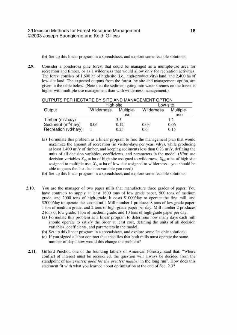
(b) Set up this linear program in a spreadsheet, and explore some feasible solutions. 2.9. Consider a ponderosa pine forest that could be managed as a multiple-use area for
recreation and timber, or as a wilderness that would allow only for recreation activities. The forest consists of 1,600 ha of high-site (i.e., high-productivity) land, and 2,400 ha of low-site land. The expected outputs from the forest, by site and management option, are given in the table below. (Note that the sediment going into water streams on the forest is higher with multiple-use management than with wilderness management.)
OUTPUTS PER HECTARE BY SITE AND MANAGEMENT OPTION High-site Low-site Output Wilderness Multiple-
use Wilderness Multiple-
use Timber (m
3/ha/y) 3.5 1.2
Sediment (m3/ha/y) 0.06 0.12 0.03 0.06
Recreation (vd/ha/y) 1 0.25 0.6 0.15
(a) Formulate this problem as a linear program to find the management plan that would maximize the amount of recreation (in visitor-days per year, vd/y), while producing at least 1,400 m3/y of timber, and keeping sediments less than 0.23 m3/y, defining the units of all decision variables, coefficients, and parameters in the model. (Hint: use decision variables Xhw = ha of high site assigned to wilderness, Xhm = ha of high site assigned to multiple use, Xlw = ha of low site assigned to wilderness – you should be able to guess the last decision variable you need)
(b) Set up this linear program in a spreadsheet, and explore some feasible solutions.
2.10. You are the manager of two paper mills that manufacture three grades of paper. You have contracts to supply at least 1600 tons of low grade paper, 500 tons of medium grade, and 2000 tons of high-grade. It costs $1000/day to operate the first mill, and $2000/day to operate the second mill. Mill number 1 produces 8 tons of low grade paper, 1 ton of medium grade, and 2 tons of high-grade paper per day. Mill number 2 produces 2 tons of low grade, 1 ton of medium grade, and 10 tons of high-grade paper per day. (a) Formulate this problem as a linear program to determine how many days each mill
should operate to satisfy the order at least cost, defining the units of all decision variables, coefficients, and parameters in the model.
(b) Set up this linear program in a spreadsheet, and explore some feasible solutions. (c) If you signed a labor contract that specifies that both mills must operate the same
number of days, how would this change the problem? 2.11. Gifford Pinchot, one of the founding fathers of American Forestry, said that: “Where
conflict of interest must be reconciled, the question will always be decided from the standpoint of the greatest good for the greatest number in the long run”. How does this statement fit with what you learned about optimization at the end of Sec. 2.3?
2/Decision Methods for Forest Resource Management ©2003 Joseph Buongiorno and Keith Gilless
19
ANNOTATED REFERENCES
Davis, L.S., K.N. Johnson, P.S. Bettinger and T.E. Howard. 2001. Forest management: To
sustain ecological, economic, and social values. McGraw-Hill, New York, New York. 804 p. (Chap. 6 discusses formulating linear programming models.)
Dykstra, D.P. 1984. Mathematical programming for natural resource management. McGraw-
Hill, New York. 318 p. (Chap. 2 presents a simple two variable land management linear programming model.)
Ells, A., E. Bulte and G.C. van Kooten. 1996. Uncertainty and forest land use allocation in
British Columbia: Vague priorities and imprecise coefficients. Forest Science 43(4):509-520. (Discusses situations in which the determinism assumption of linear programming models is problematic.)
Foster, B.B. 1969. Linear programming: A method for determining least cost blends or mixes in
papermaking. Tappi 52(9):1658-1660. (Determines the least cost blend of pulpwood species that will produce a paper with certain characteristics.)
Hanover, S.J., W.L. Hafley, A.G. Mullin, R.K. Perrin. 1973. Linear programming analysis for
hardwood dimension production. Forest Products Journal 23(11):47-50. (Determines the size and grade of lumber that will maximize the profits of a sawmill subject to technological and contractual constraints.)
Kent, B.M. 1989. Forest service land management planners' introduction to linear
programming. USDA Forest Service, General Technical Report RM-173. Fort Collins. 36 p. (Discusses simple linear programming models for forest resource management.)
Kotak, D.B. 1976. Application of linear programming to plywood manufacture. Interfaces
7(1):56-68. (Optimizes the wood mix used by a plywood mill.) Little, R.L. and T.E. Wooten. 1972. Product optimization of a log concentration yard by linear
programming. Department of Forestry, Clemson University, Clemson. Forest Research Series No. 24. 14 p. (Discusses using a linear programming model for sorting logs for resale.)
Ragsdale, C.T. 1998. Spreadsheet modeling and decision analysis: A practical introduction to
management science. South-Western College Publishing, Cincinnati. 742 p. (Chap. 2 discusses formulating linear programming models.)
Winston, W.L. 1995. Introduction to mathematical programming. Duxbury Press, Belmont. 818
p. (Chap. 3 discusses formulating linear programming models.)
3/Decision Methods for Forest Resource Management © 2003 Joseph Buongiorno and Keith Gilless
1
Chapter 3 __________________________________________________________________
Principles of Linear Programming: Solutions
After a forest management problem has been formulated as a linear program, the program must be solved to determine the most desirable management strategy. This chapter deals with two different methods of solution. The simplest procedure is graphic, but it can be used only with very small problems. Computers use a more general technique, the simplex method. After an optimum solution has been obtained, one can explore how sensitive it is to the values of the parameters in the model. To this end we shall study duality, a powerful method of sensitivity analysis in linear programming. 3.1 GRAPHIC SOLUTION OF THE POET’S PROBLEM Large linear programming models that represent real managerial problems must be solved with a computer. However, the small problem that we developed in Sec. 2.2 for the poet-forester can be solved with a simple graphic procedure. The technique illustrates well the nature of the general linear programming solution. Recall the expression of that problem:
0,
) workof days(18032
)hardwoods of ha(50
)pine red of ha (40
:Subject to
)$/yr (12090max
21
21
2
1
21
≥
≤+
≤
≤
+=
XX
XX
X
X
XXZ
Where the variable X
1 is the number of hectares of red pine that the poet should
manage, and X2 is the number of hectares of northern hardwoods. The object is to
find the values of these two variables that maximize Z, which measures the poet's annual revenue from the property. There are 40 hectares of red pine on the property and 50 hectares of hardwoods, and the poet is willing to use up to 180 days per year to manage his forest.
3/Decision Methods for Forest Resource Management © 2003 Joseph Buongiorno and Keith Gilless
2
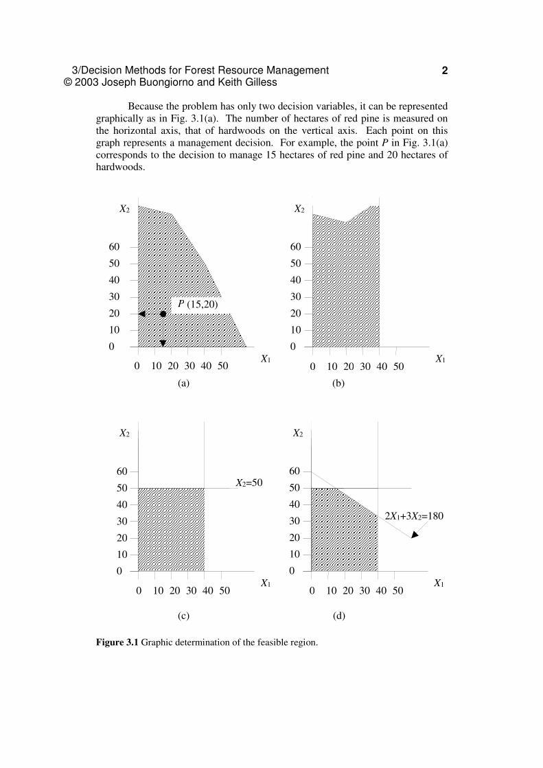
Because the problem has only two decision variables, it can be represented graphically as in Fig. 3.1(a). The number of hectares of red pine is measured on the horizontal axis, that of hardwoods on the vertical axis. Each point on this graph represents a management decision. For example, the point P in Fig. 3.1(a) corresponds to the decision to manage 15 hectares of red pine and 20 hectares of hardwoods.
Figure 3.1 Graphic determination of the feasible region.
X 1
X 2
0
20
30
40
50
60
10
P (15,20)
X 1
X 2
10 20 30 40 500X 1
X 2
X 2=50
2X 1+3X 2=180
X 1
X 2
(a) (b)
(c) (d)
10 20 30 40 500
10 20 30 40 50010 20 30 40 500
0
20
30
40
50
60
10
0
20
30
40
50
60
10
0
20
30
40
50
60
10
3/Decision Methods for Forest Resource Management © 2003 Joseph Buongiorno and Keith Gilless
3
However, given the resource constraints, not all points on the diagram correspond to a possible (feasible) decision. The first task in solving a linear program is to find all the points that are feasible; among those points we then seek the point(s) that maximize the objective function.
Feasible Region Since both X
1 and X
2 cannot be negative, only the shaded portion of Fig 3.1(a) can
contain a feasible solution. In addition, the constraint 401 ≤X means that a
feasible point (X1, X
2) cannot lie to the right of the vertical line X
1 = 40. This is
reflected in Fig. 3.3(b), where the shaded area contains only the values of X1 and
X2 that are permissible thus far.
Next, the constraint 502 ≤X eliminates all the points above the horizontal
line 502 =X ; the feasible region now consists of the points within the shaded
rectangle in Fig. 3.1(c).
The last constraint is set by the poet's time: 18032 21 ≤+ XX . Only the
points that lie on one side of the line 18032 21 =+ XX satisfy this restriction. To
plot that line on our figure, we need two of its points. For example, if X1= 0, then
X2 = 60. Similarly, if 302 =X , then 452/)90180(1 =−=X . To find on which
side of the line 18032 21 =+ XX the feasible region lies, we need to check for
one point only. For example, at the origin, both X1 and X
2 are zero and the time
constraint holds; therefore, all the points on the same side of 18032 21 =+ XX as
the origin satisfy the poet's time constraint. In summary, the feasible region is represented by the shaded polygon in
Fig. 3.1(d). The coordinates of any point within that region simultaneously satisfy the land constraints, the poet's time constraint and the non-negativity constraints. In the next step we shall determine which point(s) in the feasible region maximize the objective function.
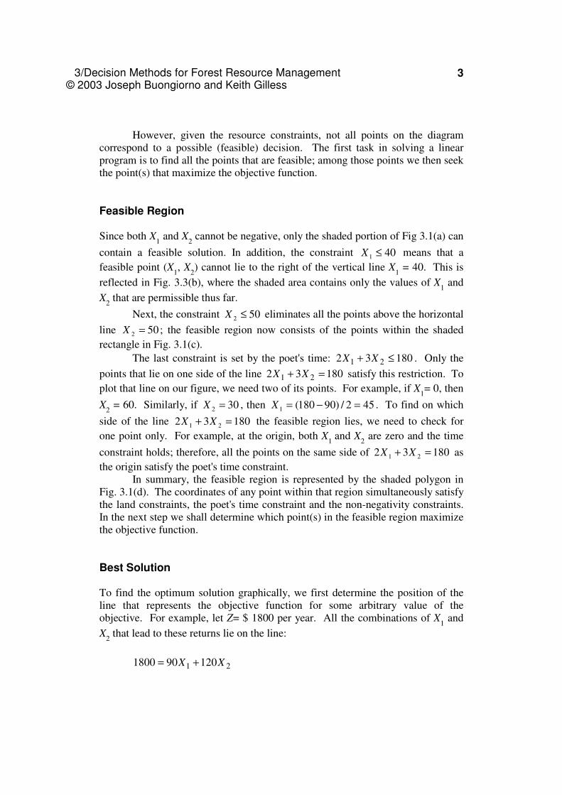
Best Solution To find the optimum solution graphically, we first determine the position of the line that represents the objective function for some arbitrary value of the objective. For example, let Z= $ 1800 per year. All the combinations of X
1 and
X2 that lead to these returns lie on the line:
21 120901800 XX +=
3/Decision Methods for Forest Resource Management © 2003 Joseph Buongiorno and Keith Gilless
4
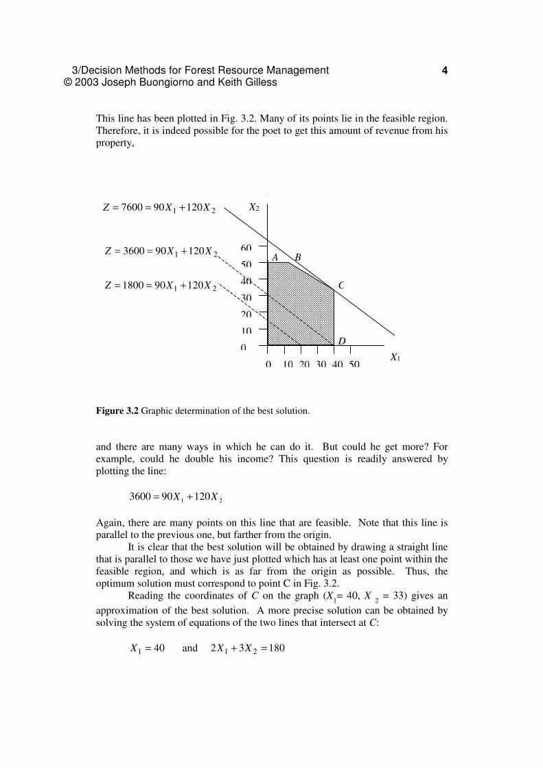
This line has been plotted in Fig. 3.2. Many of its points lie in the feasible region. Therefore, it is indeed possible for the poet to get this amount of revenue from his property,
Figure 3.2 Graphic determination of the best solution.
and there are many ways in which he can do it. But could he get more? For example, could he double his income? This question is readily answered by plotting the line:
21 120903600 XX += Again, there are many points on this line that are feasible. Note that this line is parallel to the previous one, but farther from the origin.
It is clear that the best solution will be obtained by drawing a straight line that is parallel to those we have just plotted which has at least one point within the feasible region, and which is as far from the origin as possible. Thus, the optimum solution must correspond to point C in Fig. 3.2.
Reading the coordinates of C on the graph (X1= 40, X
2 = 33) gives an
approximation of the best solution. A more precise solution can be obtained by solving the system of equations of the two lines that intersect at C:
18032 and 40 211 =+= XXX
D
C
BA
X2
X1
0
20
30
40
50
60
10
10 20 30 40 50 0
21 120907600 XXZ +==
21 120903600 XXZ +==
21 120901800 XXZ +==
3/Decision Methods for Forest Resource Management © 2003 Joseph Buongiorno and Keith Gilless
5
Therefore, the best value of X
1 is:
X1* = 40 ha
Substituting X1* in the second equation leads to:
33.333
80180*2 =
−=X ha
Therefore, the best strategy for the poet is to cultivate all the red pine he has, but only 33 ha of the hardwoods, leaving the rest idle. That it may be best in some circumstances not to use all of the available resources is an important lesson of linear programming.
The best value of the objective function; that is the maximum revenue that the poet can obtain from his land is then:
)year/($7600*120*90 21 =+ XX
Sensitivity Analysis As mentioned in Sec. 2.6, linear programming assumes that the parameters of the model are known exactly. The solution obtained above is best only if the parameters are correct. This may not be true. It is therefore useful to do a sensitivity analysis; that is to explore how the best solution changes with different values of the parameters. The simplest form of sensitivity analysis is to observe how the best solution responds to a change in one single parameter, keeping all other things equal.
For example, assume that the returns to hardwood management were $150/ha/y, instead of $120/ha/y, while everything else stays the same. Show how this would change the objective function, and lead to the best solution being at point B instead of C in Fig. 3.2. The new best solution would then be: X1*= 15 hectares of red pine, X2*=50 hectares of hardwoods, and Z*=$8,850/year of revenue.
Note that one of the resources would still not be fully used in this new best solution: the poet would now be better off by not managing 25 hectares of his red pine.
3/Decision Methods for Forest Resource Management © 2003 Joseph Buongiorno and Keith Gilless
6
3.2 GRAPHIC SOLUTION OF THE RIVER POLLUTION PROBLEM The problem of the cooperative owning the pulp mill (as described in Sec. 2.3) consisted of finding X1 and X2, the daily production of mechanical and chemical pulp, such that the river pollution from mill effluents would be as small as possible:
5.1min 21 XXZ +=
subject to:
30021 ≥+ XX (employment target, workers)
000,40200100 21 ≥+ XX (revenue target, $/day)
3001 ≤X (mechanical-pulping capacity, tons/day)
2002 ≤X (chemical-pulping capacity, tons/day)
0, 21 ≥XX
The graphic solution of this linear program proceeds as follows. There are
only two decision variables in the problem; these are measured along the axes of Fig. 3.3. We first determine the possible values of X1 and X2 (feasible region) and then find the point in this region that maximizes the objective function (best solution). Feasible Region
The nonnegativity constraints )0,0( 21 ≥≥ XX limit the possible solution to the
positive part of the plane defined by the axes in Fig. 3.3. In addition, the
employment constraint, ( 30021 ≥+ XX workers), limits the solution to the half
plane to the right of the boundary line 30021 =+ XX , which goes through the
points (X1=0, X2=300) and (X1=300, X2=0). This can be verified by observing that for any point to the left of that line, say the origin, the employment constraint is not satisfied.
The feasible region is limited further by the revenue constraint
( 000,40200100 21 ≥+ XX $/day). The boundary line of this constraint goes
through the points (X1=0, X2=200) and (X2=0, X1=400). For the origin the constraint is false; therefore the feasible region lies to the right of the boundary line.
3/Decision Methods for Forest Resource Management © 2003 Joseph Buongiorno and Keith Gilless
7
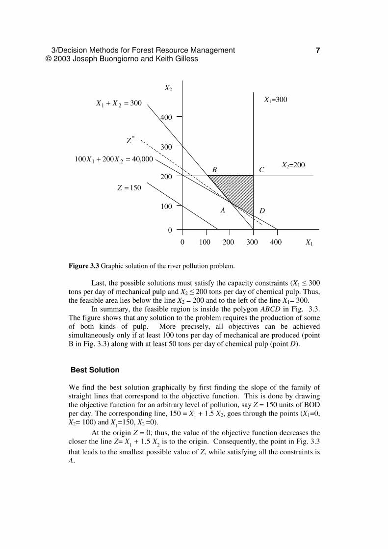
Figure 3.3 Graphic solution of the river pollution problem.
Last, the possible solutions must satisfy the capacity constraints (X1 ≤ 300
tons per day of mechanical pulp and X2 ≤ 200 tons per day of chemical pulp. Thus, the feasible area lies below the line X2 = 200 and to the left of the line X1= 300.
In summary, the feasible region is inside the polygon ABCD in Fig. 3.3. The figure shows that any solution to the problem requires the production of some of both kinds of pulp. More precisely, all objectives can be achieved simultaneously only if at least 100 tons per day of mechanical are produced (point B in Fig. 3.3) along with at least 50 tons per day of chemical pulp (point D).
Best Solution We find the best solution graphically by first finding the slope of the family of straight lines that correspond to the objective function. This is done by drawing the objective function for an arbitrary level of pollution, say Z = 150 units of BOD per day. The corresponding line, 150 = X1 + 1.5 X2, goes through the points (X1=0, X2= 100) and X
1=150, X2 =0).
At the origin Z = 0; thus, the value of the objective function decreases the closer the line Z= X
1 + 1.5 X
2 is to the origin. Consequently, the point in Fig. 3.3
that leads to the smallest possible value of Z, while satisfying all the constraints is A.
X1=300
X2=200 B
A D
C
X1
X2
100 200 300 400
100
200
300
400
0
0
30021 =+ XX
000,40200100 21 =+ XX
150=Z
*Z
3/Decision Methods for Forest Resource Management © 2003 Joseph Buongiorno and Keith Gilless
8
The coordinates of A can be read directly from the graph. Alternatively, one can solve the system of equations that define the coordinates of A, namely:
X1 + X
2 = 300 and 100 X
1 + 200 X
2 = 40,000.
We eliminate X
1 by first multiplying the first equation by 100, and then
subtracting it from the second. Solving this leads to:
X2* = 100 tons/day of chemical pulp
Substituting this result in the first equation then gives:
X1* = 200 tons/day of mechanical pulp
The value of the objective function that correspond to this optimum
operating strategy is:
Z* = X1* + 1.5 X
2* = 350 units of BOD/day
This is the minimum amount of pollution that the pulp mill can produce, while satisfying all other objectives. 3.3 THE SIMPLEX METHOD The graphic method that we have used to solve the two previous examples is limited to cases where there are at most two or three decision variables in the model. For larger problems, a more general technique is needed. The simplex method is an algebraic procedure that, when programmed on a computer, can solve problems with thousands of variables and constraints quickly and cheaply.
This section will give only an overview of the method. The objective is to show the principles involved, rather than the laborious arithmetic manipulations. The principles of the simplex are straightforward and elegant. The arithmetic is best left to a computer.
Slack Variables The first step of the simplex method is to transform all inequalities in a linear programming model into equalities. This is done because equalities are much easier to handle mathematically. In particular, a lot is known about the properties and solutions of systems of linear equations.
3/Decision Methods for Forest Resource Management © 2003 Joseph Buongiorno and Keith Gilless
9
As an example, let's recall the formulation of the poet's problem (sec. 2.2): Find the areas of red pine, X
1, and of hardwoods, X2, to manage such that:
0,
workof days18032
hardwoods of ha50
pine red of ha40
:subject to
($/yr)12090max
21
21
2
1
21
≥
≤+
≤
≤
+=
XX
XX
X
X
XXZ
The first constraint can be changed into an equality by introducing one
additional variable, S1, called a slack variable, as follows: X1 + S1 = 40 and S1 ≥ 0 Note that S1 simply measures the area of red pine that is not managed. We proceed in similar fashion with each constraint and obtain the following transformed model: Find X1, X2, S1, S2, S3 such that:
0,,,,
18032
50
40
:subject to
12090max
32121
321
22
11
21
≥
=++
=+
=+
+=
SSSXX
SXX
SX
SX
XXZ
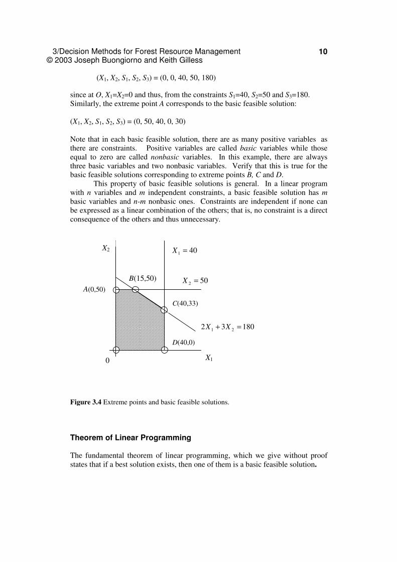
where, S2 is the slack variables measuring unused hardwoods land, and S3 is the slack variable measuring unused poet time. Basic Feasible Solutions Let us return to the geometric representation of the feasible solutions for this linear program. For convenience, it is reproduced in Fig. 3.4. The feasible region is the entire area inside the polygon OABCD. The equations of the boundary lines are shown on the figure.
A basic feasible solution of this linear program corresponds to the corners of the polygon OABCD; we shall call these corners the extreme points of the feasible region. For example, extreme point O corresponds to the basic feasible solution:
3/Decision Methods for Forest Resource Management © 2003 Joseph Buongiorno and Keith Gilless
10
(X1, X2, S1, S2, S3) = (0, 0, 40, 50, 180)
since at O, X1=X2=0 and thus, from the constraints S1=40, S2=50 and S3=180. Similarly, the extreme point A corresponds to the basic feasible solution: (X1, X2, S1, S2, S3) = (0, 50, 40, 0, 30) Note that in each basic feasible solution, there are as many positive variables as there are constraints. Positive variables are called basic variables while those equal to zero are called nonbasic variables. In this example, there are always three basic variables and two nonbasic variables. Verify that this is true for the basic feasible solutions corresponding to extreme points B, C and D.
This property of basic feasible solutions is general. In a linear program with n variables and m independent constraints, a basic feasible solution has m basic variables and n-m nonbasic ones. Constraints are independent if none can be expressed as a linear combination of the others; that is, no constraint is a direct consequence of the others and thus unnecessary.
Figure 3.4 Extreme points and basic feasible solutions.
Theorem of Linear Programming The fundamental theorem of linear programming, which we give without proof states that if a best solution exists, then one of them is a basic feasible solution.
D(40,0)
B(15,50)
X2
X1 0
18032 21 =+ XX
401 =X
C(40,33)
A(0,50)
502 =X
3/Decision Methods for Forest Resource Management © 2003 Joseph Buongiorno and Keith Gilless
11
This theorem implies that in a linear program, there may be one, many, or no solution. The theorem is fundamental because it means that to solve a linear program one needs to consider only a finite number of solutions -- the basic feasible solutions corresponding to the extreme points of the feasible region.
Since the best solution of a linear program is a basic feasible solution, it has exactly as many positive variables as there are independent constraints. If a problem has 10 independent constraints and 10,000 variables, only 10 variables in the best solution have positive values, all the rest are zero.
There may be even fewer positive variables in the best solution if all constraints are not independent. Assume there are 10 constraints in a linear program and we get only 8 positive variables in the best solution, then two of the constraints must be redundant: they result necessarily from the others, and thus they can be omitted from the model without altering the results.
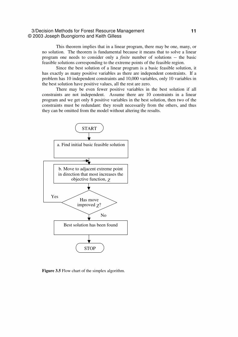
Figure 3.5 Flow chart of the simplex algorithm.
a. Find initial basic feasible solution
START
b. Move to adjacent extreme point in direction that most increases the
objective function, Z
Has move improved Z?
Best solution has been found
STOP
No
Yes
3/Decision Methods for Forest Resource Management © 2003 Joseph Buongiorno and Keith Gilless
12
Solution Algorithm Given the theorem of linear programming, a possible solution procedure (an algorithm) would be to calculate all the basic feasible solutions, and find the one that maximizes or minimizes the objective function. But this is impractical for large problems because the number of basic feasible solutions may still be too large to examine all of them, even with a fast computer.
The simplex method uses, instead, a steepest-ascent algorithm. It consists of moving from one extreme point to the next adjacent extreme point of the feasible region in the direction that improves the objective function most.
The process can be visualized in this way: Think of the feasible region as a mountain, the peak of which corresponds to the optimum solution. A climber is lost in the fog and can barely see her feet. To reach the summit, she proceeds cautiously but surely. Keeping one foot fixed at one point, she moves the other foot around her to find the direction of the next step that will raise her most. When she has found it she moves in that direction. If no step in any direction lifts the climber, she has reached the summit.
The flow chart in Fig. 3.5 summarizes the various steps of the simplex method. Step (a) consists in finding an initial feasible solution. In step (b) we move from one extreme point to an adjacent extreme point in the direction that most increases the objective function Z. If step (b) has improved the objective function, step (b) is repeated. The iterations continue until no improvement in Z occurs, indicating that the optimum solution was obtained in the penultimate iteration.
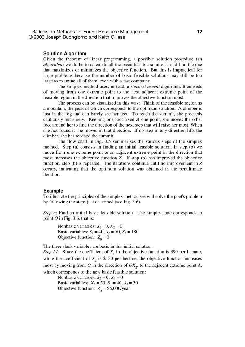
Example To illustrate the principles of the simplex method we will solve the poet's problem by following the steps just described (see Fig. 3.6). Step a: Find an initial basic feasible solution. The simplest one corresponds to point O in Fig. 3.6, that is:
Nonbasic variables: X1= 0, X2 = 0 Basic variables: S1 = 40, S2 = 50, S3 = 180 Objective function: Z
0 = 0
The three slack variables are basic in this initial solution. Step b1: Since the coefficient of X
1 in the objective function is $90 per hectare,
while the coefficient of X2 is $120 per hectare, the objective function increases
most by moving from O in the direction of OX2, to the adjacent extreme point A,
which corresponds to the new basic feasible solution: Nonbasic variables: S2 = 0, X1 = 0 Basic variables: X2 = 50, S1 = 40, S3 = 30 Objective function: Z
A = $6,000/year
3/Decision Methods for Forest Resource Management © 2003 Joseph Buongiorno and Keith Gilless
13
In the movement from extreme point O to A, the variable X
2 that was nonbasic has
become basic, and the variable S2 that was basic has become nonbasic. This is general; the algebraic equivalent of an adjacent extreme point is a basic feasible solution with a single different basic variable. The steepest ascent chooses as the new basic variable the one that increases the objective function the most.
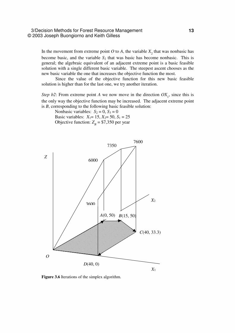
Since the value of the objective function for this new basic feasible solution is higher than for the last one, we try another iteration. Step b2: From extreme point A we now move in the direction OX
1, since this is
the only way the objective function may be increased. The adjacent extreme point is B, corresponding to the following basic feasible solution:
Nonbasic variables: S2 = 0, S3 = 0 Basic variables: X1= 15, X2= 50, S1 = 25 Objective function: Z
B = $7,350 per year
Figure 3.6 Iterations of the simplex algorithm.
B(15, 50) A(0, 50)
O
D(40, 0)
C(40, 33.3)
Z
6000
73507600
3600X2
X1
3/Decision Methods for Forest Resource Management © 2003 Joseph Buongiorno and Keith Gilless
14
Since the last iteration has increased the objective function, we try another one.
Step b3: The only way the objective function may be increased is by moving to the adjacent extreme point C, which corresponds to the basic feasible solution:
Nonbasic variables: S1 = 0, S3 = 0 Basic variables: X1= 40, X2 = 33.3, S2 =17.7 Objective function: ZC= $7,600 per year
The last iteration having increased the objective function, we try another
one.
Sep b4: The next adjacent extreme point is D, corresponding to the basic feasible solution:
Nonbasic variables: S1 = 0, X2= 0 Basic variables: X1 = 40, S2 = 50, S3 = 100 Objective function: ZD= $3,600 per year.
This iteration has decreased the value of the objective function; therefore, the optimum solution is the basic feasible solution corresponding to extreme point C, reached in the previous iteration.
3.4 DUALITY IN LINEAR PROGRAMMING Every linear programming problem has a symmetric formulation that is very useful in interpreting the solution, especially to determine how the objective function changes if one of the constraints changes slightly, everything else remaining equal. This symmetric formulation is called the dual problem. It contains exactly the same data as the original (primal) problem, but rearranged in a symmetric fashion. This different way of looking at the same data yields very useful information. General Definition Recall the standard formulation of the linear programming problem given in Chap. 2: Find X1, X2,…, Xn, all nonnegative, such that:
3/Decision Methods for Forest Resource Management © 2003 Joseph Buongiorno and Keith Gilless
15
mnmnmm
nn
nn
nn
bXaXaXa
bXaXaXa
bXaXaXa
XcXcXcZ
≤+++
≤+++
≤+++
+++=
...
...
...
...
:subject to
...max
2211
22222121
11212111
2211
The dual of this problem is a linear program with the following
characteristics: The objective function of the dual is minimized (it would be maximized if the primal problem were a minimization). It has as many variables (dual variables) as there are constraints in the primal, and all dual variables are positive or zero. It has as many constraints as there are variables in the primal.
The coefficients aij in each column of the primal problem become coefficients in corresponding rows of the dual (first column becomes first row, second column second row, etc.) The coefficients of the objective function in the primal become the coefficients on the right hand side of the constraints, and vice-versa. The direction of the inequalities is reversed.
Consequently, the dual of the standard linear program given above is to fnd Y1 to Ym, all non-negative, such that:
nmmnnn
mm
mm
mm
cYaYaYa
cYaYaYa
cYaYaYa
YbYbYbZ
≥+++
≥+++
≥+++
+++=
...
...
...
...
:subject to
...'min
2211
22222112
11221111
2211
Duality is symmetric in that the dual of the dual is the primal. You can
verify this by applying the definition of duality to the dual, thereby recovering the primal formulation.
3/Decision Methods for Forest Resource Management © 2003 Joseph Buongiorno and Keith Gilless
16
Applications of Duality The duality theorem, one of the most important of linear programming, states that a solution of the dual exists if and only if the primal has a solution. Furthermore, the optimum values of the objective functions of the primal and of the dual are
equal. In our notations, Z *=Z' *. We shall see the usefulness of this theorem in the following two examples. Dual of the Poet's Problem Recall the linear programming model we formulated for the poet who wanted to find the areas of red pine and hardwoods he should manage (X1, X2) in order to maximize his annual revenues (Z), while spending no more than half of his time in the woods.
0,
yearper work of days18032
hardwoods of ha50
pine red of ha40
:subject to
yearper $12090max
21
21
2
1
21
≥
≤+
≤
≤
+=
XX
XX
X
X
XXZ
Applying the duality definition leads to the following dual problem:
0,,
12030
9020
:subject to
1805040min
321
321
321
321
≥
≥++
≥++
++=′
YYY
YYY
YYY
YYYZ
Shadow Prices We know from Sec. 3.3 that the best value of the objective function for the primal problem is Z= $7,600 per year. The duality theorem states that the best value of the objective function of the dual must be equal to the best value of the objective function of the dual:
Z'*=Z*= $7,600 per year Thus, Z', the objective function of the dual must be measured in dollars per year. In addition, we know the units of measurement of the coefficients of the objective function of the dual because they are the coefficients of the right-hand-side of the primal. Consequently, one can infer the units of measurement of the dual variables by making the objective function of the dual homogeneous in its units. This leads to:
3/Decision Methods for Forest Resource Management © 2003 Joseph Buongiorno and Keith Gilless
17
)$/d(3
)d/y()$/ha/y(2
ha)()$/ha/y(1
)ha()$/y(1805040 YYYZ ++=′
where y and d refer to year and day, respectively. Verify that with these units for Y1, Y2 and Y3 the two constraints are also homogeneous in their units.
It is now apparent that Y1 expresses the value of using red pine land, in dollars per hectare per year. Similarly, Y2 is the value of using hardwoods land, and Y3 is the value of the poet's time in dollars per day. In linear programming terminology, Y1, Y2 and Y3 are shadow prices.
The qualifier "shadow" is a reminder that these prices are not necessarily equal to the market prices of the resources. For example, Y3 is not the value of the poet's time for hire; it is only an implicit value that reflects the activities in which the poet can engage (in this problem), managing red pine and hardwoods. The duality theorem indicates that when all resources are used in an optimal manner, the total implicit value of the resources is equal to the annual returns.
The shadow prices are very useful in getting the most out of a linear programming model. To see this, assume that the dual of the poet's problem has
been solved. Designate the value of the shadow prices at the optimum by Y1*, Y2
*
and Y3*. Then, the expression of the objective function of the dual problem at the
optimum is:
)$/d(3
)d/y()$/ha/y(2
ha)()$/ha/y(1
)ha()$/y(*180*50*40* YYYZ ++=′
Thus, if the red pine land available increased or decreased by one hectare (from 40 to 41 or 39 ha) while the amounts of hardwoods land and poet time remained
fixed, the objective function would increase or decrease by Y1* ($/y). Similarly, if
the amount of hardwoods land available changed from 50 to 51 or 49 ha, the objective function would increase or decrease by Y2* ($/y). And, if the amount of time available to the poet increased or decreased by 1 day per year, the objective function would increase or decrease by Y3* ($/y).
In summary, the shadow prices measure by how much the best value of the objective function would change if the right-hand side of a constraint changed by one unit, other things being equal.
To obtain the shadow prices it is not necessary to formulate and solve the dual separately. Modern versions of the simplex method give simultaneously the optimal primal and dual solution. The next section shows how to get the dual solution with the Excel Solver. It turns out that the shadow prices for the poet’s problem are:
Y1*=10 ($/year/ha of red pine)
Y2*=0 ($/year/ha of hardwoods)
Y3*=40 ($/day of poet's time)
3/Decision Methods for Forest Resource Management © 2003 Joseph Buongiorno and Keith Gilless
18
These shadow prices show that one additional hectare of land would increase the poet's annual revenues by $10. On the other hand, extra hardwoods would be worth nothing. This is consistent with the fact that in the best primal solution we found that about 16.7 ha of hardwoods were not used. The third shadow price shows that one additional day working in the woods is worth $40 to the poet. This is the most revenue that he could get by managing his woods optimally with that additional time. This information should be most useful for the poet to decide if the financial and aesthetic benefits of versification are worth that much.
In interpreting dual solutions, keep in mind that shadow prices are strictly marginal values. They measure changes in the objective function that result from small changes in each of the constraints. For example, in the poet's problem, the
shadow price Y2* is zero as long as the hardwoods constraint is not binding. The
best solution found in Sec. 3.3 showed that 16.7 ha of hardwoods should be left idle. Thus, were the poet to sell more than 16.7 ha of his land, the hardwoods
constraint would become binding, and the shadow price Y2* would become
positive. Dual of the River Pollution Problem In using the shadow prices of a linear program one must keep in mind the direction of the inequalities, and whether the objective function is minimized or maximized. As an example of a slightly more involved interpretation of shadow prices, let us recall the river pollution problem formulated in Sec. 2.3. The primal problem was: Find X1 and X2, the tonnages of mechanical and chemical pulp produced daily, such that:
0,
) t/dcapacity, pulping chemical(200
) t/dcapacity, pulping mechanical(300
$) revenue,daily (000,40200100
employed) workers(300
:subject to
day)per BOD of units(5.1min
21
2
1
21
21
21
≥
≤
≤
≥+
≥+
+=
XX
X
X
XX
XX
XXZ
This primal problem is not in the standard format, so that the interpretation of the shadow prices requires some care.
Solving the river pollution problem with a computer program (see next section) gives the following shadow prices:
Y1* = 0.5 (BOD units/day/worker)
Y2* = 0.005 (BOD units/$)
Y3* = 0 (BOD units/ton)
3/Decision Methods for Forest Resource Management © 2003 Joseph Buongiorno and Keith Gilless
19
Y4* = 0 (BOD units/ton)
We have inferred the units of each shadow price by dividing the unit of the objective function by the units of the constraint to which the shadow price applies.
The two easiest shadow prices to interpret are Y3* and Y
4*. They are
both zero because at the optimum solution there is excess capacity for both pulp- making processes. This can be checked in Fig. 3.3. Additional capacity would have no effect on pollution.
The workers’ constraint is binding. Its shadow price shows that pollution would increase by 0.5 units of BOD per day for each additional worker that the cooperative might employ. Similarly, pollution would increase by 0.005 units of BOD for each additional dollar of daily revenues that the cooperative earned.
In many linear programming problems, some careful thinking will bring useful information out of the dual solution. Nevertheless, there are situations in which the shadow prices are either difficult to interpret or do not have any economic meaning because of the structure of the problem.
3.5 SPREADSHEET SOLUTION OF LINEAR PROGRAMS In Sec. 2.5 we learned how to formulate linear programming problems with a computer spreadsheet, and to use the spreadsheet to explore the effects of different choices of variables. We can then use the Solver optimization program of Excel to find the best solution. Spreadsheet Solution of the Poet’s Problem
To invoke the Solver in Excel, choose the Solver command from the Tools menu. This displays a Solver Parameters dialog box. The Solver Parameters dialog box with the parameters for the poet’s problem is shown in Fig. 3.7. The target cell, D10, is the cell that contains the objective function in the spreadsheet formulation of the poet’s problem.
Clicking on the Max button directs the Solver to maximize the objective function. The Solver seeks the best solution by changing cells B3:C3, which contain the two decision variables.
The first line in the Subject to the Constraints window shows that the decision variables must be nonnegative. The second line indicates that the cells D6:D8 must be less than or equal than the corresponding cells F6:F8. This means that the red pine land managed must be at most 40 ha, the hardwoods land managed must be at most 50 ha, and the poet’s time used must be at most 180
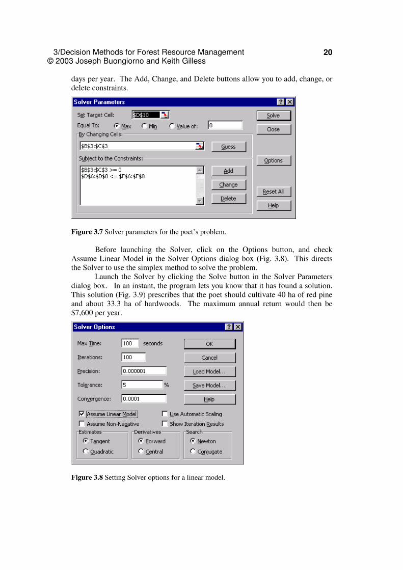
3/Decision Methods for Forest Resource Management © 2003 Joseph Buongiorno and Keith Gilless
20
days per year. The Add, Change, and Delete buttons allow you to add, change, or delete constraints.
Figure 3.7 Solver parameters for the poet’s problem.
Before launching the Solver, click on the Options button, and check
Assume Linear Model in the Solver Options dialog box (Fig. 3.8). This directs the Solver to use the simplex method to solve the problem.
Launch the Solver by clicking the Solve button in the Solver Parameters dialog box. In an instant, the program lets you know that it has found a solution. This solution (Fig. 3.9) prescribes that the poet should cultivate 40 ha of red pine and about 33.3 ha of hardwoods. The maximum annual return would then be $7,600 per year.
Figure 3.8 Setting Solver options for a linear model.
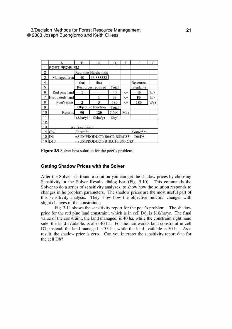
3/Decision Methods for Forest Resource Management © 2003 Joseph Buongiorno and Keith Gilless
21
1
2
3
4
5
6
7
8
9
10
11
12
13
14
15
16
A B C D E F G
POET PROBLEM
Red pine Hardwoods
Managed area 40 33.333333
(ha) (ha) Resources
Total available
Red pine land 1 40 <= 40 (ha)
Hardwoods land 1 33 <= 50 (ha)
Poet's time 2 3 180 <= 180 (d/y)
Total
Returns 90 120 7,600 Max
($/ha/y) ($/ha/y) ($/y)
Key Formulas
Cell Formula Copied to
D6 =SUMPRODUCT(B6:C6,B$3:C$3) D6:D8
D10 =SUMPRODUCT(B10:C10,B$3:C$3)
Resources required
Objective function
Figure 3.9 Solver best solution for the poet’s problem.
Getting Shadow Prices with the Solver
After the Solver has found a solution you can get the shadow prices by choosing Sensitivity in the Solver Results dialog box (Fig. 3.10). This commands the Solver to do a series of sensitivity analyzes, to show how the solution responds to changes in he problem parameters. The shadow prices are the most useful part of this sensitivity analysis. They show how the objective function changes with slight changes of the constraints.
Fig. 3.11 shows the sensitivity report for the poet’s problem. The shadow price for the red pine land constraint, which is in cell D6, is $10/ha/yr. The final value of the constraint, the land managed, is 40 ha, while the constraint right hand side, the land available, is also 40 ha. For the hardwoods land constraint in cell D7, instead, the land managed is 33 ha, while the land available is 50 ha. As a result, the shadow price is zero. Can you interpret the sensitivity report data for the cell D8?
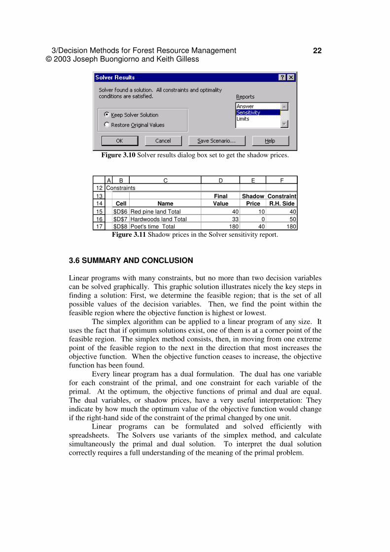
3/Decision Methods for Forest Resource Management © 2003 Joseph Buongiorno and Keith Gilless
22
Figure 3.10 Solver results dialog box set to get the shadow prices.
12
13
14
15
16
17
A B C D E F
Constraints
Final Shadow Constraint
Cell Name Value Price R.H. Side
$D$6 Red pine land Total 40 10 40
$D$7 Hardwoods land Total 33 0 50
$D$8 Poet's time Total 180 40 180 Figure 3.11 Shadow prices in the Solver sensitivity report.
3.6 SUMMARY AND CONCLUSION Linear programs with many constraints, but no more than two decision variables can be solved graphically. This graphic solution illustrates nicely the key steps in finding a solution: First, we determine the feasible region; that is the set of all possible values of the decision variables. Then, we find the point within the feasible region where the objective function is highest or lowest.
The simplex algorithm can be applied to a linear program of any size. It uses the fact that if optimum solutions exist, one of them is at a corner point of the feasible region. The simplex method consists, then, in moving from one extreme point of the feasible region to the next in the direction that most increases the objective function. When the objective function ceases to increase, the objective function has been found.
Every linear program has a dual formulation. The dual has one variable for each constraint of the primal, and one constraint for each variable of the primal. At the optimum, the objective functions of primal and dual are equal. The dual variables, or shadow prices, have a very useful interpretation: They indicate by how much the optimum value of the objective function would change if the right-hand side of the constraint of the primal changed by one unit.
Linear programs can be formulated and solved efficiently with spreadsheets. The Solvers use variants of the simplex method, and calculate simultaneously the primal and dual solution. To interpret the dual solution correctly requires a full understanding of the meaning of the primal problem.
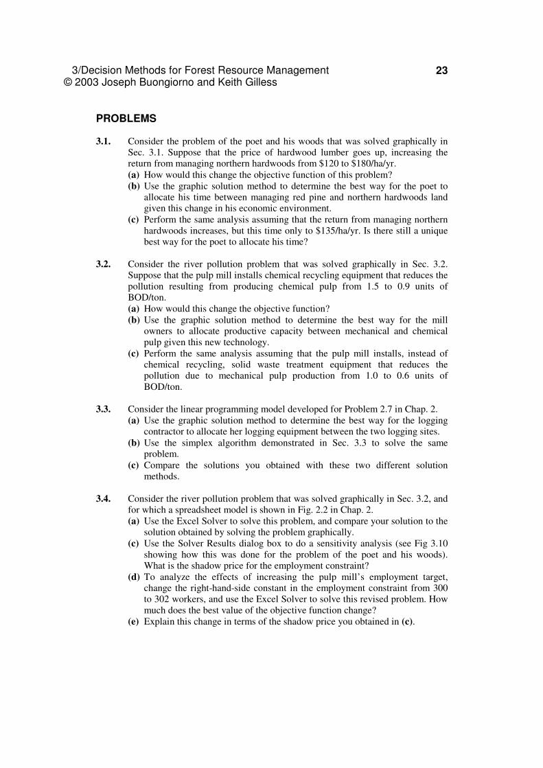
3/Decision Methods for Forest Resource Management © 2003 Joseph Buongiorno and Keith Gilless
23
PROBLEMS
3.1. Consider the problem of the poet and his woods that was solved graphically in
Sec. 3.1. Suppose that the price of hardwood lumber goes up, increasing the return from managing northern hardwoods from $120 to $180/ha/yr. (a) How would this change the objective function of this problem? (b) Use the graphic solution method to determine the best way for the poet to
allocate his time between managing red pine and northern hardwoods land given this change in his economic environment.
(c) Perform the same analysis assuming that the return from managing northern hardwoods increases, but this time only to $135/ha/yr. Is there still a unique best way for the poet to allocate his time?
3.2. Consider the river pollution problem that was solved graphically in Sec. 3.2.
Suppose that the pulp mill installs chemical recycling equipment that reduces the pollution resulting from producing chemical pulp from 1.5 to 0.9 units of BOD/ton. (a) How would this change the objective function? (b) Use the graphic solution method to determine the best way for the mill
owners to allocate productive capacity between mechanical and chemical pulp given this new technology.
(c) Perform the same analysis assuming that the pulp mill installs, instead of chemical recycling, solid waste treatment equipment that reduces the pollution due to mechanical pulp production from 1.0 to 0.6 units of BOD/ton.
3.3. Consider the linear programming model developed for Problem 2.7 in Chap. 2.
(a) Use the graphic solution method to determine the best way for the logging contractor to allocate her logging equipment between the two logging sites.
(b) Use the simplex algorithm demonstrated in Sec. 3.3 to solve the same problem.
(c) Compare the solutions you obtained with these two different solution methods.
3.4. Consider the river pollution problem that was solved graphically in Sec. 3.2, and for which a spreadsheet model is shown in Fig. 2.2 in Chap. 2. (a) Use the Excel Solver to solve this problem, and compare your solution to the
solution obtained by solving the problem graphically. (c) Use the Solver Results dialog box to do a sensitivity analysis (see Fig 3.10
showing how this was done for the problem of the poet and his woods). What is the shadow price for the employment constraint?
(d) To analyze the effects of increasing the pulp mill’s employment target, change the right-hand-side constant in the employment constraint from 300 to 302 workers, and use the Excel Solver to solve this revised problem. How much does the best value of the objective function change?
(e) Explain this change in terms of the shadow price you obtained in (c).
3/Decision Methods for Forest Resource Management © 2003 Joseph Buongiorno and Keith Gilless
24
3.5. Consider the problem of the poet and his woods, for which a spreadsheet model is shown in Fig. 2.1 and Excel Solver parameters are shown in Fig. 3.7. The dual of this problem was solved in Sec. 3.4, and shadow prices for the constraints are shown in Fig. 3.11. (a) Assume that the poet is willing to spend more time managing his forest.
Change the right-hand-side constant in the time constraint from 180 to 182 days, then use the Excel Solver to solve this revised problem. How much does the best value of the objective function change?
(b) Explain this change in terms of the fact that the shadow price for the poet’s time constraint in the original problem was $40/day.
(c) Assume that the poet is considering buying more land. Change the right-hand-side constant in the hardwood land constraint from 50 ha to 55 ha, then use the Excel Solver to solve this revised problem. How much does the best value of the objective function change?
(d) Explain this change in terms of the fact that the shadow price for the northern hardwoods land constraint in the original problem was $0/ha.
ANNOTATED REFERENCES
Blanning, R.W. 1974. The sources and uses of sensitivity information. Interfaces
4(4):32-38. (Describes four different methods of evaluating the sensitivity of a model to its parameters.)
Davis, L.S., K.N. Johnson, P.S. Bettinger and T.E. Howard. 2001. Forest management:
To sustain ecological, economic, and social values. McGraw-Hill, New York. 804 p. (Chap. 6 discusses solving linear programming models.)
Hof, J., M. Bevers and J. Pickens. 1995. Pragmatic approaches to optimization with
random yield coefficients. Forest Science 41(3):501-512. (Discusses several ways to account for uncertainty in harvest yields in linear programming models.)
Kent, B.M. 1989. Forest service land management planners' introduction to linear
programming. USDA Forest Service, Gen. Tech. Report RM-173. Fort Collins. 36 p. (Discusses simple linear programming models for forest resource management.)
Perry, C. and K.C. Crellin. 1982. The precise management meaning of a shadow price.
Interfaces 12(2):61-63. (Precise explanation of shadow prices and how they can be used in decision-making.)
Ragsdale, C.T. 1998. Spreadsheet modeling and decision analysis: A practical
introduction to management science. South-Western College Publishing, Cincinnati. 742 p. (Chaps. 2 and 3 discuss solving linear programming models graphically and with spreadsheets, and Chap. 4 discusses sensitivity analysis of solutions.)
3/Decision Methods for Forest Resource Management © 2003 Joseph Buongiorno and Keith Gilless
25
Weintraub, A. and A. Abramovich. 1995. Analysis of uncertainty of future timber yields in forest management. Forest Science 41(2):217-234. (Discusses an approach to handling uncertainty in harvest yields in linear programming models by formulating constraints as probability statements.)
Winston, W.L. 1995. Introduction to mathematical programming. Duxbury Press,
Belmont. 818 p. (Chap. 4 discusses solving linear programming models, and Chaps. 5 and 6 discuss sensitivity analysis of solutions.)