UPTEC F15030

Examensarbete 30 hpJuni 2015

Tuning for Ride Quality in Autonomous Vehicle Application to Linear Quadratic

Path Planning Algorithm

Jenny ErikssonLars Svensson

Teknisk- naturvetenskaplig fakultet UTH-enheten Besöksadress: Ångströmlaboratoriet Lägerhyddsvägen 1 Hus 4, Plan 0 Postadress: Box 536 751 21 Uppsala Telefon: 018 – 471 30 03 Telefax: 018 – 471 30 00 Hemsida: http://www.teknat.uu.se/student

Abstract

Tuning for Ride Quality in Autonomous Vehicle

Jenny Eriksson, Lars Svensson

When introducing autonomous functionality in personal vehicles the ability to control the quality of the ride is transferred from the driver to the vehicle control system. In this context, a reference method for quantifying ride quality may be a useful tool in the development and tuning process.

This master’s thesis investigates whether general quantitative measures of ride quality can be of value in the tuning of motion controllers for autonomous vehicles. A set of tools is built for a specific case study, analyzing a lateral path planning algorithm, based on a finite horizon linear quadratic tracking controller, and how its tuning affects ride quality performance.

A graphical user interface is built, with functionality for frequency domain analysis of the path planning algorithm, individually and in combination with the remaining lateral control system, as well as ride quality evaluation based on lateral acceleration data, from logged test runs and simulation results. In addition, a simulation environment for the lateral control system is modified to be used in combination with the evaluation tool. Results of the case study indicate a measurable difference in ride quality performance when comparing manual and autonomous driving with the current implementation. Attempts were made to improve ride quality by re-tuning the path planning algorithm but little or no improvement from the previous tuning was made.

The work has recognized the potential of using ride quality measures in the development and tuning process for autonomous vehicles as well as devising a tuning strategy incorporating frequency analysis and ride quality evaluation through simulation for the lateral control system. To further increase ride quality performance via the path planning algorithm an altered controller structure, such as a frequency weighted linear quadratic controller is suggested.

ISSN: 1401-5757, UPTEC F15030Examinator: Tomas NybergÄmnesgranskare: Thomas SchönHandledare: Mohammad Ali

Sammanfattning

Vid inforandet av autonoma personbilar overfors ansvaret att astadkomma en behagligkorupplevelse fran foraren till bilens styrsystem, med hoga krav pa komfort som foljd.Syftet med denna studie ar att integrera metoder for att utvardera akkomfort direkt i al-goritminstallningen for autonoma bilar. Detta har gjorts via utveckling av ett verktyg somspecifikt har tagits fram for en lateral vagplaneringsalgoritm baserad pa linjarkvadratiskservoreglering, LQT.

Verktyget innehaller tre separata funktionaliteter: simulering, komfortutvardering ochfrekvensdomansanalys. Simuleringsmiljon har tagits fram for att generera rorelsedata vidgivna referenssituationer. Rorelsedatat har senare kunnat anvandas i verktygets komfort-utvardering. Det bestar av ett flertal metoder for evaluering av komfort och illamaende ochar resultatet av en litteraturstudie. Verktygets tredje funktion, frekvensdomansanalysen,ger en mojlighet att direkt kunna avgora hur olika frekvenser forstarks och dampas i detlaterala styrsystemet. Via det sammansatta verktyget har tydliga slutsatser kunnat drasom hur olika installningar paverkar bilbeteende.

Tester i bil visade en matbar skillnad i komfort och aksjuka nar man jamfor autonomoch manuell korning. Forsok gjordes for att forbattra den nuvarande installningen, utanframgang. Vidare undersokning antydde att de modeller som anvandes i verktyget varotillrackliga. For att avgora hur val strategin i sig fungerar behovs fler tester i bil samtbattre indata vid simulering.

Studien har uppmarksammat potentialen i att anvanda komfortmatt i utvecklingen ochinstallningen av algoritmer for autonoma bilar. En strategi har utformats for hur mankan anvanda frekvensdomansanalys och komfortevaluering av simulerad data i install-ningsprocessen. For vidare forbattring av komfort via vagplaneraren foreslas en ny regu-latorstruktur med storre designfrihet, till exempel en frekvensviktad linjarkvadratisk reg-ulator (FSLQ)

v

Acknowledgements

First of all we would like to thank Volvo for giving us the opportunity to carry out thismaster’s thesis work. It has been a great pleasure to take part in such high-technologydevelopment. A special thanks goes out to Mohammad Ali, our supervisor at Volvo whocame up with the idea for this thesis and has provided us with many theoretical insightswithin control theory. It is safe to say that we have learned a lot. The friendly atmosphereat Decision and Control has encouraged us to reach out for help and second opinions fromother colleagues within the department, we are sincerely grateful for you taking the timeeven when our projects were quite separated. Furthermore we would like to thank oursupervisor at Uppsala University, Thomas Schon, for all valuable comments and guidelinesfor improving the quality of this thesis. Hans Norlander was also very kind to thoroughlyread the report and give constructive feedback which was much appreciated in the processof refining the report.

Finally, we would like to add how tremendous it has been to spend the last few monthswith our new friends in Gothenburg. We were told that there is nothing like a spring inGothenburg and we quite agree.

Uppsala, June 2015Jenny and Lars

viii

Notationz , Reference vector for path planning algorithm

u , System control signal vector

x , State vector in path planning algorithm

yT /yP , lateral position of trail/path

ΨT /ΨP , Heading of trail/path

ΨT /ΨP , Yaw rate of trail/path

κT , Curvature of trail

Vx , Longitudinal velocity in vehicle’s coordinate system

δwheel,des , Desired front wheel steering angle

δwheel , Front wheel steering angle

Ψinj , Desired yaw rate of vehicle

∆y , Lateral error with respect to desired path

∆Ψ , Yaw angle error with respect to desired path

yL2 , Lateral error at lookahead point

Leff , Look ahead distance

Ψ , Yaw rate of vehicle

Ψinj , Disturbance on yawrate error with respect to desired path

∆yinj , Disturbance on lateral error with respect to desired path

Y , Global position of car

x , Longitudinal axis

y , Lateral axis

z , Vertical axis

ai,Wj (t) , Frequency weighted acceleration time series

ai,Wj ,rms , RMS of frequency weighted acceleration time series

ai,Wj ,P95 , 95ht percentile of frequency weighted acceleration

Tf , Time range of acceleration data

Wb , Weighting function for ISO 2631-4 comfort measure

Wc , Weighting function for CEN 12299 comfort measure

Wd , Weighting function for ISO 2631-1 comfort measure

Wf , Weighting function for ISO 2631-1 motion sickness measure

MSDV , Motion sickness dose value, ISO 2631-1

Km , Gain factor for motion sickness dose value

NV A , Mean comfort complete method score CEN 12299

UIC rq note , Ride quality score of UIC’s combined method

y50 , 50th percentile of lateral acceleration data

ix

Abbreviations

AD Autonomous drivingMD Manual DrivingLQR Linear quadratic regulatorLQT Linear quadratic tracking controllerFSLQ Frequency shaped linear quadratic controllerSPAS Extensive simulation environment used for validationMSDV Motion sickness dose valuePSD Power spectral densityFFT Fast Fourier transformSISO Single input single output

xi

Contents

1 Introduction 11.1 Background . . . . . . . . . . . . . . . . . . . . . . . . . . . . . . . . . . . . 11.2 Objectives . . . . . . . . . . . . . . . . . . . . . . . . . . . . . . . . . . . . . 21.3 Contributions . . . . . . . . . . . . . . . . . . . . . . . . . . . . . . . . . . . 21.4 Thesis outline . . . . . . . . . . . . . . . . . . . . . . . . . . . . . . . . . . . 3

2 Ride Quality Evaluation 42.1 Introduction to ride quality . . . . . . . . . . . . . . . . . . . . . . . . . . . 4

2.1.1 Definitions . . . . . . . . . . . . . . . . . . . . . . . . . . . . . . . . 42.1.2 Limitations . . . . . . . . . . . . . . . . . . . . . . . . . . . . . . . . 52.1.3 Published work . . . . . . . . . . . . . . . . . . . . . . . . . . . . . . 5

2.2 Description of evaluation methods . . . . . . . . . . . . . . . . . . . . . . . 52.2.1 Maximum values of acceleration and jerk . . . . . . . . . . . . . . . 62.2.2 Frequency content of acceleration . . . . . . . . . . . . . . . . . . . . 62.2.3 ISO 2631 . . . . . . . . . . . . . . . . . . . . . . . . . . . . . . . . . 72.2.4 UIC ride quality note . . . . . . . . . . . . . . . . . . . . . . . . . . 92.2.5 Summary of evaluation methods . . . . . . . . . . . . . . . . . . . . 9

2.3 Validation of methods for autonomous vehicle . . . . . . . . . . . . . . . . . 102.4 Usability . . . . . . . . . . . . . . . . . . . . . . . . . . . . . . . . . . . . . . 12

3 System description 143.1 Path planning algorithm . . . . . . . . . . . . . . . . . . . . . . . . . . . . . 15

3.1.1 Input data . . . . . . . . . . . . . . . . . . . . . . . . . . . . . . . . 153.1.2 Vehicle model . . . . . . . . . . . . . . . . . . . . . . . . . . . . . . . 163.1.3 LQT control algorithm . . . . . . . . . . . . . . . . . . . . . . . . . . 173.1.4 Initiation . . . . . . . . . . . . . . . . . . . . . . . . . . . . . . . . . 19

3.2 Lateral controller . . . . . . . . . . . . . . . . . . . . . . . . . . . . . . . . . 19

4 Simulation of the lateral control system 204.1 Vehicle model in simulation environment . . . . . . . . . . . . . . . . . . . . 204.2 Implementation . . . . . . . . . . . . . . . . . . . . . . . . . . . . . . . . . . 214.3 Validation . . . . . . . . . . . . . . . . . . . . . . . . . . . . . . . . . . . . . 224.4 Usability . . . . . . . . . . . . . . . . . . . . . . . . . . . . . . . . . . . . . . 22

xiii

5 Frequency domain analysis 245.1 Approximating the path planning algorithm . . . . . . . . . . . . . . . . . . 25

5.1.1 Reduced LQT . . . . . . . . . . . . . . . . . . . . . . . . . . . . . . . 255.1.2 LQR . . . . . . . . . . . . . . . . . . . . . . . . . . . . . . . . . . . . 265.1.3 Comparison of the approximations . . . . . . . . . . . . . . . . . . . 29

5.2 Full lateral system . . . . . . . . . . . . . . . . . . . . . . . . . . . . . . . . 305.2.1 Lateral controller, actuators and car model . . . . . . . . . . . . . . 315.2.2 Connecting the path planner to the remaining lateral system . . . . 31

5.3 Validation . . . . . . . . . . . . . . . . . . . . . . . . . . . . . . . . . . . . . 335.4 Usability . . . . . . . . . . . . . . . . . . . . . . . . . . . . . . . . . . . . . . 33

6 Experiments and results 366.1 Comparing manual and autonomous driving . . . . . . . . . . . . . . . . . . 366.2 Understanding the tuning parameters . . . . . . . . . . . . . . . . . . . . . 37

6.2.1 Effects of altering individual tuning parameters . . . . . . . . . . . . 386.2.2 Effects of altering multiple tuning parameters . . . . . . . . . . . . . 39

6.3 Evaluation of new tuning sets . . . . . . . . . . . . . . . . . . . . . . . . . . 446.3.1 Frequency analysis of new tuning . . . . . . . . . . . . . . . . . . . . 446.3.2 Simulation with new tuning . . . . . . . . . . . . . . . . . . . . . . . 456.3.3 Vehicle test with new tuning . . . . . . . . . . . . . . . . . . . . . . 456.3.4 Simulation with new tuning on logged drivable area trail input . . . 47

7 Concluding remarks 507.1 Conclusions . . . . . . . . . . . . . . . . . . . . . . . . . . . . . . . . . . . . 507.2 Ideas for further development . . . . . . . . . . . . . . . . . . . . . . . . . . 52

8 References 53

Appendices 55

A Preparation of data 56A.1 Acceleration and Jerk . . . . . . . . . . . . . . . . . . . . . . . . . . . . . . 56

A.1.1 The Rauch-Tung-Striebel (RTS) formulas . . . . . . . . . . . . . . . 56A.2 ISO and UIC filters . . . . . . . . . . . . . . . . . . . . . . . . . . . . . . . . 57

A.2.1 ISO 2631-1 filters . . . . . . . . . . . . . . . . . . . . . . . . . . . . . 57A.2.2 ISO 2631-4 filter . . . . . . . . . . . . . . . . . . . . . . . . . . . . . 58

A.3 UIC ride quality note . . . . . . . . . . . . . . . . . . . . . . . . . . . . . . . 59

B Display of graphical tuning tool 60

xiv

1Introduction

When launching autonomous cars the driver goes from full flexibility of influencing thestyle of driving to almost none. This lays the responsibility of generating comfortablerides on the development engineers. By developing a new strategy for how to tune a pathplanning algorithm that is based not only on responsiveness but also on ride quality itshould be possible to reduce vehicle motion causing for example motion sickness. Throughdevelopment of a tool to evaluate the algorithm based on these qualities the tuning processto find an optimal trade off between responsiveness and ride quality could be significantlyshortened. Rather than having to test the different tunings in the car the developer canimmediately determine the impact of modifying the tuning directly in the tool.

1.1 Background

Driver-less vehicles have been present in most people’s lives for decades through the worldof science fiction. However, autonomous vehicles are no longer restricted to fiction, butsomething that will in the near future be made available to the public. In fact, the tran-sition to autonomous driving has been going on for quite some time. Technology likeanti-lock breaking system (ABS), electronic stability control and power steering are allexcellent examples of assisted driving taking us towards full automation. Developmentwithin driver-less vehicles goes back to the 1920’s when an empty car was placed in trafficin Milwaukee, controlled through radio waves from a following vehicle. This was of coursenot left unnoticed by the local paper, warning the people of Milwaukee of this car ”haunt-ing the streets” [23]. It seems however as the daunting message did not scare people off,in 1987 the German engineer Ernst Dickmanns and his team successfully drove the firstautomated van on an empty highway in speeds up to 96 km/h. The development of therobotic car, under the name VaMoRs, continued to advance, allowing for lane changes andsensing of other vehicles [24]. Nowadays, all major car manufacturers are developing au-

1

tonomous cars, with the expectations to soon have them commercialised. There is alreadytechnology on the market for collision avoidance, adaptive cruise control and lane keep-ing assist. The next step facing most manufacturers, as defined by the National HighwayTraffic Safety Administration in America [21], is to have a vehicle operating autonomouslyunder certain conditions, with a present driver required to retake control in a ”sufficientlycomfortable transition time” when needed. At Volvo, a project named DriveMe was initi-ated in 2014 with the aim to fulfill this level of autonomy by having 100 cars put in trafficin the city of Gothenburg by 2017 [22]. The last step towards full autonomy is a vehicleperforming all safety-critical driving functions, provided navigation inputs, both occupiedand unoccupied.

The possible benefits of autonomous driving are many, including less car accidents, lesspollution, reduced traffic congestion and less space needed for infrastructure. However,once the technology is developed for having autonomous cars out in traffic the challengestill remains to convince the people of the advantages. Most importantly the passengerneeds to feel safe and comfortable. When he or she has little or no direct influence on thecontrol of the car, it is of vital importance that the autonomous system is set to generatemovements that are perceived as pleasant. Therefore, studying effects of vehicle mo-tion on human beings might be crucial for the car manufacturers developing autonomouscars.

1.2 Objectives

The main objective of this thesis has been to develop a new strategy for tuning of a lateralpath planner used in autonomous cars at Volvo. The idea was to put greater emphasis onthe ride quality caused by the tuning rather than solely considering tracking properties. AMATLAB tool was to be developed that could evaluate for these characteristics. Thereforethe thesis was organized into three areas of focus:

• Literature study on how to evaluate ride quality from motion data.

• Development of simulation environment to enable generation of system response fordifferent road scenarios.

• Frequency domain analysis of the path planning algorithm and its effect on thevehicle response.

The idea was that when integrating these analyses in one tool it would be possible to makea decision on tuning parameters from inspection of both frequency domain characteristicsas well as ride quality performance of simulated runs.

1.3 Contributions

The main contribution of this thesis is a conceptual strategy for incorporating quantifiedride quality measures in the tuning process of motion controllers in autonomous vehicles.The strategy utilizes classical control theory methods as well as batch simulation to find

2

tuning parameter sets that will evade undesired frequency content in the vehicle acceler-ation if possible. Applying the methods to frequency weighted control algorithms wouldbe an interesting continuation.

1.4 Thesis outline

The thesis is organized into six chapters excluding this one. Chapter 2 defines the termride quality and introduces methods of evaluating it. The lateral control system, whichthe path planning algorithm is part of, is described in Chapter 3 to supply the reader withbackground on how the current system works. This system was modelled and implementedas a simulation environment, which is described in Chapter 4. In Chapter 5 the methodsof deriving the mathematical expressions of the path planner system and the full lateralsystem are presented and evaluated. This chapter contains a discussion of how this partof the tool was useful. In Chapter 6 methods and results of using the tuning tool arepresented and discussed. The discussion of the performance of the tuning tool continuesin Chapter 7 where also some ideas for further work are presented.

3

2Ride Quality Evaluation

The main objective of this thesis has been to find methods for incorporating ride qualityevaluation in the tuning process of the lateral path planner. Several methods for evaluatingride quality have been found and compared for application to autonomous cars. Thefollowing section introduces the term ride quality and methods for evaluating it, as wellas some initial results on logged data.

2.1 Introduction to ride quality

A driver feeling discomfort can easily adjust his or her style of driving to feel more atease. At the introduction of autonomous functionality this ability is transferred to the carcontrol system. In order to achieve a comfortable ride in an autonomous vehicle, methodsof evaluating ride quality are required. Several studies exists that have been made totry to map different parameters to a perceived ride quality. Even though it is a highlysubjective measure literature states that it is possible to trace ride quality perception tocertain parameter values.

2.1.1 Definitions

Ride quality is a term describing a person’s subjective perception of a vehicle ride. Poorride quality gives rise to passenger discomfort and sometimes motion sickness. Good ridequality is associated with passenger comfort and small risk of motion sickness. Comfortis a general feeling of well-being while motion sickness is associated with dizziness, fatigueand nausea.

4

2.1.2 Limitations

There are many parameters that can affect ride quality. Besides motion variables param-eters like temperature, posture and smell can have have a significant impact. The level ofdiscomfort and motion sickness is also dependent on the individual. For example it hasbeen shown that there is a noticeable difference when comparing both gender and age. Inthis thesis however only the effect of motion variables will be considered since the otherparameters are not affected by the maneuvring of the vehicle. Moreover, impact frommotion in the lateral direction will be the main focus since this thesis is regarding a lateralpath planner.

2.1.3 Published work

There is not much published material within ride quality evaluation for autonomous driv-ing. However, for other means of transportation, a large amount of results can be found.The public transportation sector has been especially ambitious in publishing reports, sincethey want to satisfy their customers with an enjoyable ride. There are a few suggestionson how to mathematically determine ride quality from logged motion data. A commonmethod is described in an international standard, ISO2631, which determines the effectof vibrations on the human body [1]. This standard has been further extended by otherresearch groups to include a broader variety of motions. An international project underthe name UIC Comfort Tests carried out on behalf of the international Union of Railways,Banverket and Vinnova has performed a regression analysis of perceived ride quality intrains from their own experiments and added that to the ISO2631 method [10]. A researchgroup for public transportation at the KTH Royal Institute of Technology in Stockholmhas contributed with an evaluation method for ride quality on buses, which was alsodeveloped through regression analysis from experiment data [9].

2.2 Description of evaluation methods

When evaluating ride quality it is important to consider both discrete events and averagevehicle motion. Motion sickness is induced by low frequent motions over a longer periodof time while a passenger can experience discomfort from a single event, for example anabrupt lane change. As stated by Forsteberg in [4], analysis of peak and average motiondata is necessary for a full estimate of ride quality and the methods in this thesis havebeen chosen thereafter.

Documentation on limits for magnitudes and frequencies of different motion variables havebeen collected and are described in Section 2.2.1 and 2.2.2. The international standardISO 2631 contains methods for evaluating average comfort which have been widely usedby researchers and vehicle designers, they are described in Section 2.2.3. The standardcan be used individually or in combination with peak values in order to achieve a morecomplete ride quality estimate, described further in Section 2.2.4.

5

2.2.1 Maximum values of acceleration and jerk

Studies show that it is acceleration and its time derivative, jerk, that affect ride quality.Jerk typically arises at swift lane changes and entrances and exits of curves. A high valueof acceleration or jerk can cause discomfort even during shorter periods of time. Whenthe levels get too high the passenger will find it difficult to maintain posture. Thereforeit is advised to set restrictions on magnitudes of acceleration and jerk. Limit values varybetween the studies but they fall within the same range. Most of these studies are carriedout on behalf of the railway industry but since motion has the same impact on a passengerregardless of the type of vehicle these sources are considered relevant.

For acceleration the threshold for discomfort lies around 1 m/s2, ranging up to 1.47 m/s2

in the study of Baybura et al, [8]. According to Kottenhoff, [9], bus traffic usually acceptshigher levels, up to 2 m/s2 in order to follow the rhythm of the traffic.

The jerk threshold for discomfort lies around 0.5 m/s3, ranging up to 0.9m/s3 as seen in[8] and [4].

Some of these thresholds are however determined by including both seated and standingpassengers. A standing passenger in a train or on a bus has more difficulty to keep balancethrough high values of acceleration and jerk than a seated passenger. Since an automobileonly carries seated passengers it is expected that the thresholds should be set on the higherside. For acceleration it might be reasonable to set the limit closer to 2 m/s2 and jerk to0.9 m/s3.

2.2.2 Frequency content of acceleration

Low frequent motion is the main contributor to motion sickness while high frequent motioncauses stress and discomfort. Modern roads and car suspension systems are designed not togive rise to high frequent motion but low frequent behaviour may arise for example duringrepeated lane changes or breaking maneuvres. The frequency content of acceleration datacan be determined by estimation and inspection of its spectrum. For this thesis the powerspectral density, PSD, has been used.

For motion sickness, horizontal acceleration in the frequency range 0.1-0.5 Hz has the mosteffect [13], [12]. Within this range 0.2 Hz is specifically pointed out in several studies, forexample in [4], [7] and [5]. It also seems that lateral movement has greater impact onmotion sickness than longitudinal movement [5].

Higher frequencies have a negative impact on a passenger’s ability to read and write.Experimental studies in a lab environment conducted by Sundstrom et. al, [11], haveshown that for lateral vibration 2.5 Hz is critical for passengers leaning back in the seatwhile 4-5 Hz is critical when leaning forward without back support. Another experimentalstudy by Hayward et. al, [6], shows that for longitudinal vibration, also known as fore-and-aft motion, 4 Hz has the greatest impact on a passenger leaning back in the seat.

One explanation for the connection between discomfort and spectral content is that thehuman organs are put under stress when falling into resonance. The ear’s balance organ

6

undergoes resonance at frequencies below 1 Hz which might be the reason for motionsickness [9].

2.2.3 ISO 2631

ISO 2631 describes ways to evaluate vibration exposure to the human body. It definesmethods for measurement of vibrations as well as how to process measurement data tostandardized quantified performance measures concerning health, perception, comfort andmotion sickness. The standard is applicable to situations in vehicles, buildings and in thevicinity of machinery. ISO 2631-1, [1], describes general methods and the related standarddocuments ISO 2631-2 through ISO 2631-5 describes the specifics of different applicationsof the methods. ISO 2631-4, [2], specifically describes the application of the ISO 2634-1methods to railway vehicles, which was also relevant for this study.

The quantified performance measures of ISO 2631 are based on frequency weighted rootmean square, RMS, computations of acceleration data. A performance measure for thelateral direction can be calculated as

ay,Wi,rms =

(1

Tf

∫ Tf

0a2y,Wi

(t)dt

) 12

, (2.1)

where Tf denotes the time range of the measurement, Wi denotes a frequency weightedfunction, ay,Wi(t) denotes filtered lateral acceleration and ay,Wi,rms denotes the root meansquare of ay,Wi(t) which is the score value of the method.

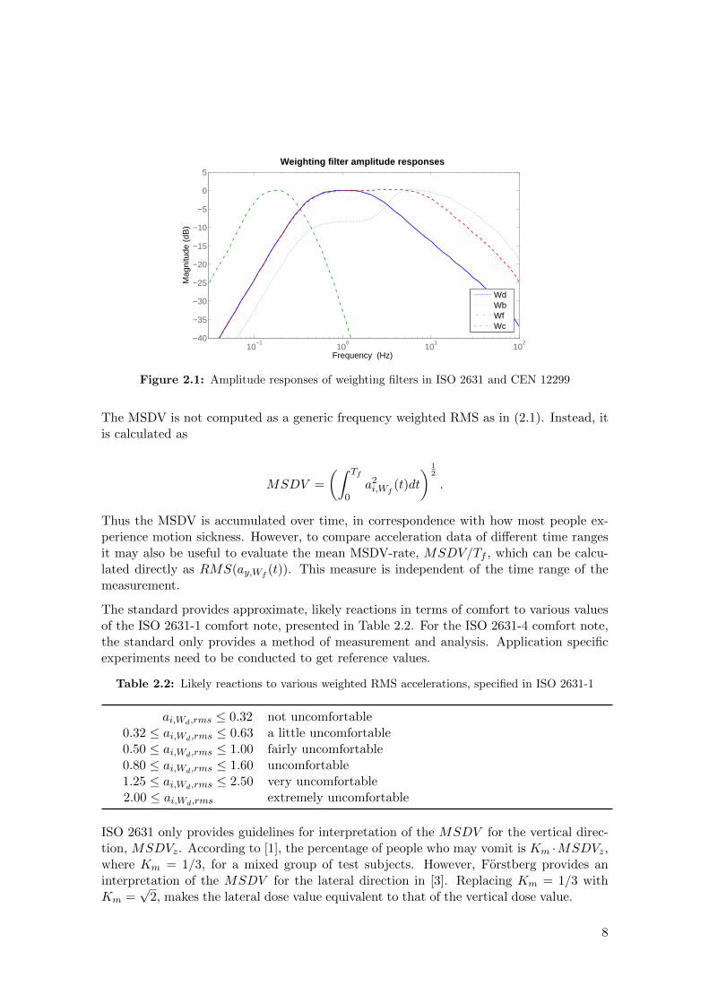
Each performance measure is related to a specific frequency weighting function. For thisstudy three performance measures from ISO 2631 have been focused. Table 2.1 displaysthe notation of the measures and their corresponding frequency weighting functions. Am-plitude responses of the weighting functions are displayed in Figure 2.1.

Table 2.1: Notation for performance measures and frequency weighting functions for ISO 2631

Performance measure notation frequency weighting function

ISO 2631-1 ay,Wd,rms Wd

ISO 2631-4 ay,Wb,rms Wb

MSDV MSDV Wf

The ISO 2631-1 comfort note is a general comfort performance measure while the ISO2631-4 comfort note was specifically developed for rail vehicle applications. MSDV isan abbreviation of motion sickness dose value and is a measure of the likelihood of nau-sea.

7

10−1

100

101

102

−40

−35

−30

−25

−20

−15

−10

−5

0

5M

agni

tude

(dB

)

Weighting filter amplitude responses

Frequency (Hz)

WdWbWfWc

Figure 2.1: Amplitude responses of weighting filters in ISO 2631 and CEN 12299

The MSDV is not computed as a generic frequency weighted RMS as in (2.1). Instead, itis calculated as

MSDV =

(∫ Tf

0a2i,Wf

(t)dt

) 12

.

Thus the MSDV is accumulated over time, in correspondence with how most people ex-perience motion sickness. However, to compare acceleration data of different time rangesit may also be useful to evaluate the mean MSDV-rate, MSDV/Tf , which can be calcu-lated directly as RMS(ay,Wf

(t)). This measure is independent of the time range of themeasurement.

The standard provides approximate, likely reactions in terms of comfort to various valuesof the ISO 2631-1 comfort note, presented in Table 2.2. For the ISO 2631-4 comfort note,the standard only provides a method of measurement and analysis. Application specificexperiments need to be conducted to get reference values.

Table 2.2: Likely reactions to various weighted RMS accelerations, specified in ISO 2631-1

ai,Wd,rms ≤ 0.32 not uncomfortable0.32 ≤ ai,Wd,rms ≤ 0.63 a little uncomfortable0.50 ≤ ai,Wd,rms ≤ 1.00 fairly uncomfortable0.80 ≤ ai,Wd,rms ≤ 1.60 uncomfortable1.25 ≤ ai,Wd,rms ≤ 2.50 very uncomfortable2.00 ≤ ai,Wd,rms extremely uncomfortable

ISO 2631 only provides guidelines for interpretation of the MSDV for the vertical direc-tion, MSDVz. According to [1], the percentage of people who may vomit is Km ·MSDVz,where Km = 1/3, for a mixed group of test subjects. However, Forstberg provides aninterpretation of the MSDV for the lateral direction in [3]. Replacing Km = 1/3 withKm =

√2, makes the lateral dose value equivalent to that of the vertical dose value.

8

ISO 2631 recommends acceleration measurements conducted on the surfaces supportinga person’s weight. For this study however, measurements have been made using sensorsbuilt into the car body, thus assuming that the seats accelerate in sync with the rest ofthe car.

The methods described in ISO 2631 are applicable to several types of vehicles but onlyfor fairly straight lines of motion. Due to the fact that the measures are evaluated as timeaverages some situations require additional methods to evaluate for transient motionsmotivating complementary analysis as concluded by Lauriks in [10].

2.2.4 UIC ride quality note

Since ISO 2631 is primarily developed for straight roads further research has been requiredto get an evaluation method covering more road scenarios. By extending the standardswith absolute measures of acceleration and jerk curvaceous roads can be included in theevaluation.

One thorough study, [10], commissioned by the International Union of Railways (UIC),has done a regression analysis of ride quality for several motion parameters for 38 peopleon 64 different rides. The best fitting equation gives a score in the interval 0-5, with 5corresponding to a highly uncomfortable ride, according to

UIC rq note = 0.094NV A + 0.6y50 + 0.37...y 50 + 0.11θ,

where y is the lateral acceleration and...y is the lateral jerk of the car body. y50 denotes

the 50th percentile of lateral acceleration. θ is the angular velocity but since roll motionis negligible in cars the term can be excluded. NV A is from a European standard namedCEN 12299. It is described according to

NV A = 4 · az,Wb,P95 + 2 ·√a2y,Wd,P95 + a2z,Wb,P95 + 4 · ax,Wc,P95

where ai,Wj ,P95 denotes the 95th percentile of acceleration data along the i axis filteredwith the weighting function Wj . The frequency weights, Wj , for CEN 12299 are the sameas for ISO 2631 (Wd and Wb) with the addition of Wc. The amplitude response of all theweighting filters are illustrated in Figure 2.1.

2.2.5 Summary of evaluation methods

To evaluate local comfort the methods that should be used are maximum acceleration andmaximum jerk. For average comfort ISO 2631 comfort note, UIC ride quality note andthe PSD method should be evaluated. Risk of nausea should be evaluated with MSDVand the PSD method.

Acceleration and jerk are the two motion variables affecting ride quality. To minimizerisk of motion sickness frequencies in the range of 0.1-0.5 Hz should be suppressed. Local

9

discomfort typically arises when the acceleration reaches 2 m/s2 or when the jerk reaches0.9 m/s3. The average ride quality can be determined by using the standard ISO 2631 orthe UIC ride quality note which evaluates the acceleration data over time.

2.3 Validation of methods for autonomous vehicle

Prior to using the methods for ride quality evaluation to tune the LQ algorithm theyneeded to be validated. Acceleration was logged for a set of different driving situationswhere it was known whether the methods should yield a high or low score on ride quality.This was compared to the passengers subjective perception of the ride.

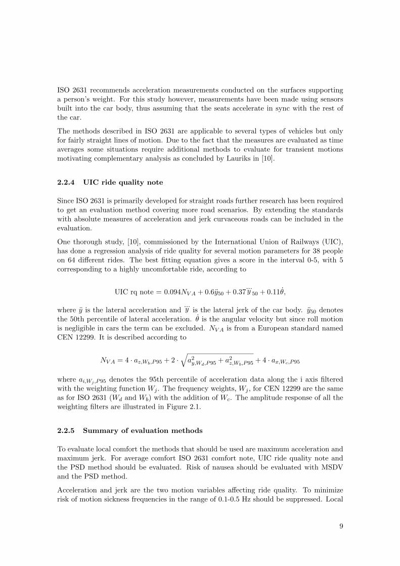
The lateral acceleration profiles for the driving situations can be viewed in Figure 2.2.They were chosen to test the methods sensibility to high levels of acceleration and jerk,oscillating driving and fairly straight driving. The data length is short since the strategywas to single out specific events that should have an impact on the methods. Some of thedata is therefore not representative of a normal ride but should merely be regarded as ameans to validate whether the methods functioned as designed.

time (s)0 5 10

acce

lera

tio

n (

m/s

2)

-5

0

5

Acceleration data for slow lane change

time (s)0 5 10

acce

lera

tio

n (

m/s

2)

-5

0

5

Acceleration data for swift lane change

time (s)0 20 40

acce

lera

tio

n (

m/s

2)

-5

0

5

Acceleration data for sinus road

time (s)0 100 200 300

acce

lera

tio

n (

m/s

2)

-5

0

5

Acceleration data for straight line

Figure 2.2: Log data used for validation of ride quality measures.

The results of applying the different ride quality measures on log data from the fourdifferent driving situations are displayed in Table 2.3 and Figure 2.3. The passengers sittingin the car when collecting the log data perceived the slow lane change as comfortable, theswift lane change as very uncomfortable and the straight road driving as very comfortable.

10

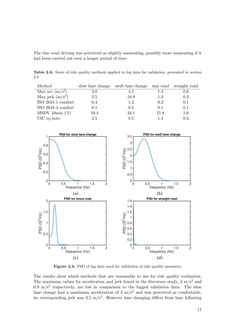
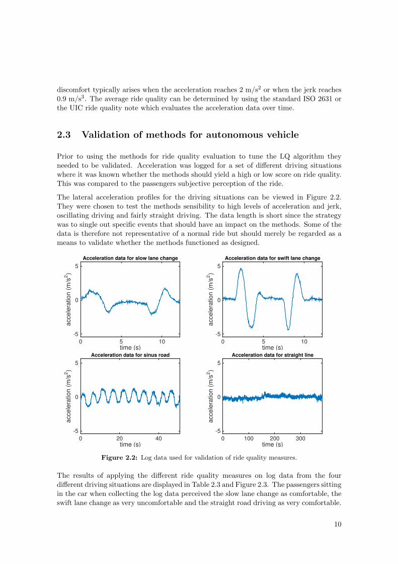
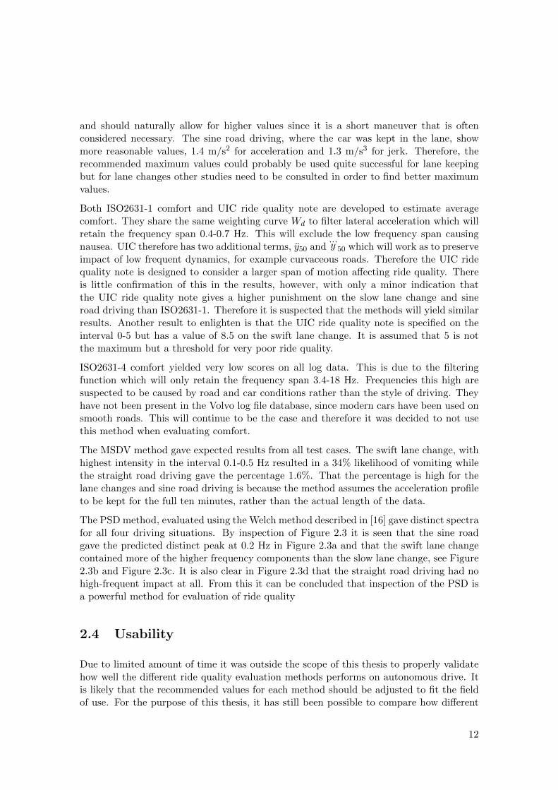
The sine road driving was perceived as slightly nauseating, possibly more nauseating if ithad been carried out over a longer period of time.

Table 2.3: Score of ride quality methods applied to log data for validation, presented in section2.3

Method slow lane change swift lane change sine road straight road

Max acc (m/s2) 2.0 4.5 1.4 0.6Max jerk (m/s3) 3.5 10.9 1.3 0.3ISO 2631-1 comfort 0.4 1.2 0.2 0.1ISO 2631-4 comfort 0.1 0.5 0.1 0.1MSDV 10min (%) 19.4 34.1 21.8 1.6UIC rq note 2.5 8.5 1.4 0.3

frequency (Hz)0 0.5 1 1.5 2

PS

D (

G2/H

z)

0

0.2

0.4

0.6

0.8

1PSD for slow lane change

(a)

frequency (Hz)0 0.5 1 1.5 2

PS

D (

G2/H

z)

0

0.5

1

1.5

2

2.5

3

3.5PSD for swift lane change

(b)

frequency (Hz)0 0.5 1 1.5 2

PS

D (

G2/H

z)

0

0.5

1

1.5

2PSD for sinus road

(c)

frequency (Hz)0 0.5 1 1.5 2

PS

D (

G2/H

z)

0

0.2

0.4

0.6

0.8

1

1.2

1.4

1.6PSD for straight road

(d)

Figure 2.3: PSD of log data used for validation of ride quality measures.

The results show which methods that are reasonable to use for ride quality evaluation.The maximum values for acceleration and jerk found in the literature study, 2 m/s2 and0.9 m/s3 respectively, are low in comparison to the logged validation data. The slowlane change had a maximum acceleration of 2 m/s2 and was perceived as comfortable,its corresponding jerk was 3.5 m/s3. However lane changing differs from lane following

11

and should naturally allow for higher values since it is a short maneuver that is oftenconsidered necessary. The sine road driving, where the car was kept in the lane, showmore reasonable values, 1.4 m/s2 for acceleration and 1.3 m/s3 for jerk. Therefore, therecommended maximum values could probably be used quite successful for lane keepingbut for lane changes other studies need to be consulted in order to find better maximumvalues.

Both ISO2631-1 comfort and UIC ride quality note are developed to estimate averagecomfort. They share the same weighting curve Wd to filter lateral acceleration which willretain the frequency span 0.4-0.7 Hz. This will exclude the low frequency span causingnausea. UIC therefore has two additional terms, y50 and

...y 50 which will work as to preserve

impact of low frequent dynamics, for example curvaceous roads. Therefore the UIC ridequality note is designed to consider a larger span of motion affecting ride quality. Thereis little confirmation of this in the results, however, with only a minor indication thatthe UIC ride quality note gives a higher punishment on the slow lane change and sineroad driving than ISO2631-1. Therefore it is suspected that the methods will yield similarresults. Another result to enlighten is that the UIC ride quality note is specified on theinterval 0-5 but has a value of 8.5 on the swift lane change. It is assumed that 5 is notthe maximum but a threshold for very poor ride quality.

ISO2631-4 comfort yielded very low scores on all log data. This is due to the filteringfunction which will only retain the frequency span 3.4-18 Hz. Frequencies this high aresuspected to be caused by road and car conditions rather than the style of driving. Theyhave not been present in the Volvo log file database, since modern cars have been used onsmooth roads. This will continue to be the case and therefore it was decided to not usethis method when evaluating comfort.

The MSDV method gave expected results from all test cases. The swift lane change, withhighest intensity in the interval 0.1-0.5 Hz resulted in a 34% likelihood of vomiting whilethe straight road driving gave the percentage 1.6%. That the percentage is high for thelane changes and sine road driving is because the method assumes the acceleration profileto be kept for the full ten minutes, rather than the actual length of the data.

The PSD method, evaluated using the Welch method described in [16] gave distinct spectrafor all four driving situations. By inspection of Figure 2.3 it is seen that the sine roadgave the predicted distinct peak at 0.2 Hz in Figure 2.3a and that the swift lane changecontained more of the higher frequency components than the slow lane change, see Figure2.3b and Figure 2.3c. It is also clear in Figure 2.3d that the straight road driving had nohigh-frequent impact at all. From this it can be concluded that inspection of the PSD isa powerful method for evaluation of ride quality

2.4 Usability

Due to limited amount of time it was outside the scope of this thesis to properly validatehow well the different ride quality evaluation methods performs on autonomous drive. Itis likely that the recommended values for each method should be adjusted to fit the fieldof use. For the purpose of this thesis, it has still been possible to compare how different

12

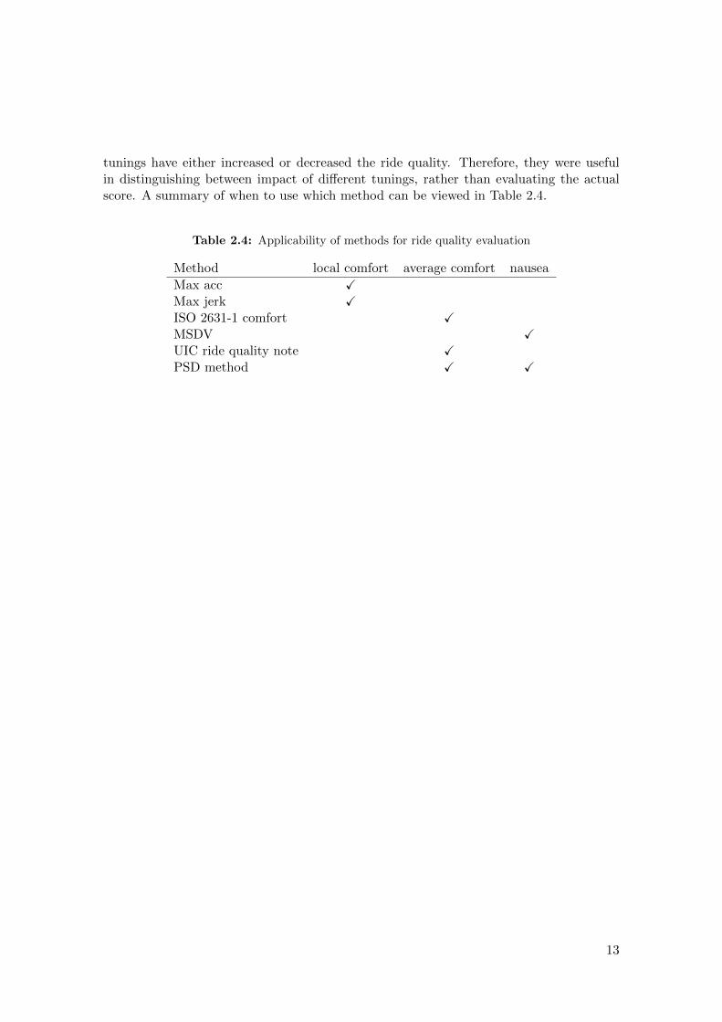
tunings have either increased or decreased the ride quality. Therefore, they were usefulin distinguishing between impact of different tunings, rather than evaluating the actualscore. A summary of when to use which method can be viewed in Table 2.4.

Table 2.4: Applicability of methods for ride quality evaluation

Method local comfort average comfort nausea

Max acc XMax jerk XISO 2631-1 comfort XMSDV XUIC ride quality note XPSD method X X

13

3System description

This chapter aims to put the path planning algorithm in a context by describing the lat-eral control system in its separate components. Development in the Drive Me project isdivided into seven areas: sensing system, sensor fusion, decision and control, architectureand system solution, human factors, dependability, vehicle build and integration and ver-ification. Of these, sensing system, sensor fusion and decision and control are directlyrelated to the car control system.

The sensing system development area deals with evaluating and integrating feasible sensingsolutions for the car. The current sensing system includes cameras, radars, laser sensingsystems and GPS. Sensor fusion deals with the problem of extracting relevant informationsuch as map position, vehicle state, road lanes, other vehicles, pedestrians etc. fromsensor data. The decision and control development area contains the longitudinal andlateral control systems of the car as well as tactical decision making such as when to dolane changes and setting reference speed. This thesis work belongs to the decision andcontrol development area and specifically deals with the lateral control system.

The lateral control system concept consist of two major components, the path planningalgorithm and the lateral controller. In general terms the purpose of the path planningalgorithm is to continuously transform a road geometry into a kinematically feasible paththat the car can follow. The path is then passed to the lateral controller which calculateswhat steering action is to be taken in order for the car to follow the path. A simplifiedoverview of the lateral control system is illustrated in Figure 3.1.

Although this thesis work is focused on analysing the behaviour of the path planningalgorithm, the dynamics of the lateral controller and the vehicle as well as the sensorfusion output, must be taken into account in order to see how the tuning of the algorithmaffects vehicle motion.

14

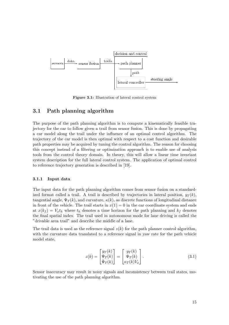
Figure 3.1: Illustration of lateral control system

3.1 Path planning algorithm

The purpose of the path planning algorithm is to compute a kinematically feasible tra-jectory for the car to follow given a trail from sensor fusion. This is done by propagatinga car model along the trail under the influence of an optimal control algorithm. Thetrajectory of the car model is then optimal with respect to a cost function and desirablepath properties may be acquired by tuning the control algorithm. The reason for choosingthis concept instead of a filtering or optimization approach is to enable use of analysistools from the control theory domain. In theory, this will allow a linear time invariantsystem description for the full lateral control system. The application of optimal controlto reference trajectory generation is described in [19].

3.1.1 Input data

The input data for the path planning algorithm comes from sensor fusion on a standard-ized format called a trail. A trail is described by trajectories in lateral position, yT (k),tangential angle, ΨT (k), and curvature, κ(k), as discrete functions of longitudinal distancein front of the vehicle. The trail starts in x(1) = 0 in the car coordinate system and endsat x(kf ) = Vxth where th denotes a time horizon for the path planning and kf denotesthe final spatial index. The trail used in autonomous mode for lane driving is called the”drivable area trail” and describe the middle of a lane.

The trail data is used as the reference signal z(k) for the path planner control algorithm,with the curvature data translated to a reference signal in yaw rate for the path vehiclemodel state,

z(k) =

yT (k)ΨT (k)

ΨT (k)

=

yT (k)ΨT (k)κT (k)Vx

. (3.1)

Sensor inaccuracy may result in noisy signals and inconsistency between trail states, mo-tivating the use of the path planning algorithm.

15

3.1.2 Vehicle model

A three state vehicle model inspired by [20] is used in the path planning algorithm. Themodel is complex enough to catch the dominating lateral dynamics of a vehicle but islimited to three states to limit computational complexity. The basis for the vehicle modelis the differential equation

y = Vx tan(Ψ) ≈ VxΨ, (3.2)

which is derived from the mechanical situation of Figure 3.2.

x

y

V

Vx

y

Ψ

Figure 3.2: Simplified lateral dynamics relations used in the car model of the path planningalgorithm

Under the assumption that the yaw acceleration is controlled, u(t) = ψ(t), a continuoustime state space model based on (3.2) can be set up as

x(t) = Actx(t) +Bctu(t),

y(t) = Cctx(t),

where the path state vector is

x(t) =

yP (t)ΨP (t)

ΨP (t)

, (3.3)

and the matrices are given by

Act =

0 Vx 00 0 10 0 0

, Bct =

001

, Cct =

1 0 00 1 00 0 1

.Assuming constant longitudinal velocity allows a description in space rather than time,

16

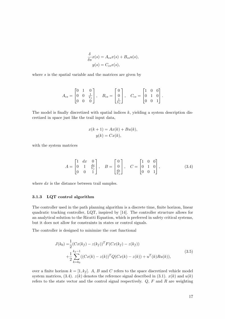
δ

δsx(s) = Acsx(s) +Bcsu(s),

y(s) = Ccsx(s),

where s is the spatial variable and the matrices are given by

Acs =

0 1 00 0 1

Vx

0 0 0

, Bcs =

001Vx

, Ccs =

1 0 00 1 00 0 1

.The model is finally discretized with spatial indices k, yielding a system description dis-cretized in space just like the trail input data,

x(k + 1) = Ax(k) +Bu(k),

y(k) = Cx(k),

with the system matrices

A =

1 dx 0

0 1 dxVx

0 0 1

, B =

00dxVx

, C =

1 0 00 1 00 0 1

, (3.4)

where dx is the distance between trail samples.

3.1.3 LQT control algorithm

The controller used in the path planning algorithm is a discrete time, finite horizon, linearquadratic tracking controller, LQT, inspired by [14]. The controller structure allows foran analytical solution to the Ricatti Equation, which is preferred in safety critical systems,but it does not allow for constraints in states or control signals.

The controller is designed to minimize the cost functional

J(k0) =1

2(Cx(kf )− z(kf ))TF (Cx(kf )− z(kf ))

+1

2

kf−1∑k=k0

((Cx(k)− z(k))TQ(Cx(k)− z(k)) + uT (k)Ru(k)),(3.5)

over a finite horizon k = [1, kf ]. A, B and C refers to the space discretized vehicle modelsystem matrices, (3.4). z(k) denotes the reference signal described in (3.1). x(k) and u(k)refers to the state vector and the control signal respectively. Q, F and R are weighting

17

matrices used to tune the controller. Tuning the controller allows system designers tomanipulate properties of the output path.

The minimization of (3.5) is achieved by solving the Ricatti difference equation

P (k) = ATP (k + 1)(I + EP (k + 1))−1A+ V,

V = CTQC,

E = BR−1BT ,

(3.6)

and the co-state difference equation

g(k) = Mgg(k + 1) +Wz(k),

Mg = AT (I − (P−1(k + 1) + E)−1E),

W = CTQ,

(3.7)

in the reverse direction, from the initial conditions

P (kf ) = CTFC,

g(kf ) = CTFz(kf ).(3.8)

The optimal state feedback, L(k), and feedforward, Lg(k), can then be computed as

L(k) = (R+BTP (k + 1)B)−1BTP (k + 1)A,

Lg(k) = (R+BTP (k + 1)B)−1BT

Note that the resulting L and Lg will be discrete functions of k, as opposed to the infinitetime LQ controller, where they are constant.

The optimal control is given by

u∗(k) = −L(k)x∗(k) + Lg(k)g(k + 1),

and the optimal state trajectory by

x∗(k + 1) = (A−BL(k))x∗(k) +BLg(k)g(k + 1).

The state trajectory is stored and made available as a reference path for the lateral con-troller.

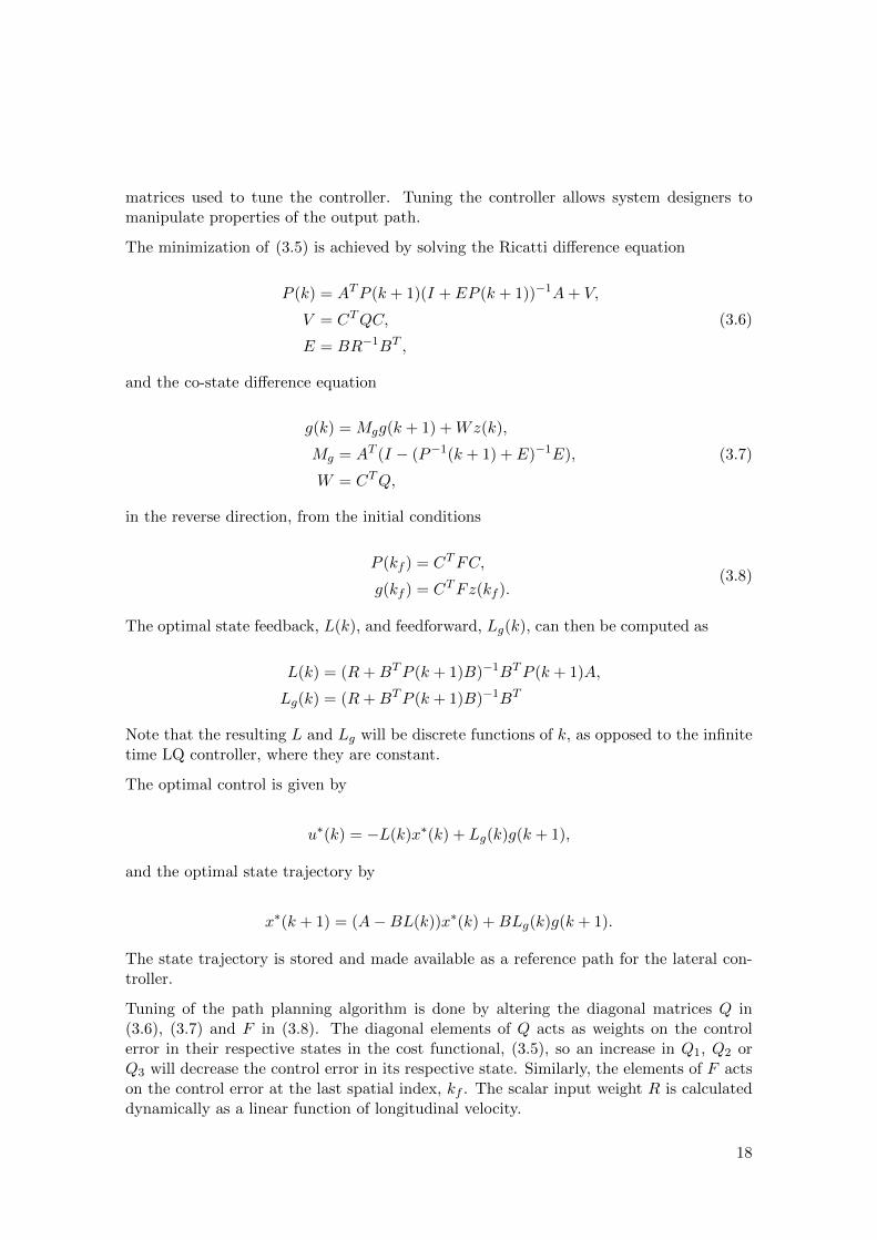
Tuning of the path planning algorithm is done by altering the diagonal matrices Q in(3.6), (3.7) and F in (3.8). The diagonal elements of Q acts as weights on the controlerror in their respective states in the cost functional, (3.5), so an increase in Q1, Q2 orQ3 will decrease the control error in its respective state. Similarly, the elements of F actson the control error at the last spatial index, kf . The scalar input weight R is calculateddynamically as a linear function of longitudinal velocity.

18

3.1.4 Initiation

The path must be updated continuously, due to the limited range of the sensors. In thecurrent implementation, the path planner is reinitialized in every iteration of the controlalgorithm, subsequently at a rate of 40 Hz. The objective is to have the path planner workas a filter on the trail data rather than be part of the controller dynamics. To achieve this,the initiation of the path planner vehicle model has to be independent of the current carposition. In the current implementation, the path from the previous time sample is storedand transformed to the current car coordinate system. Then the old path is interpolatedat x = 0 in the current coordinate system giving the initial state x(1) for the next path.The fact there is no feedback from the vehicle state to the path planner input provideda basis for how to set up the frequency analysis of the lateral control system, furtherdescribed in Section 5.

3.2 Lateral controller

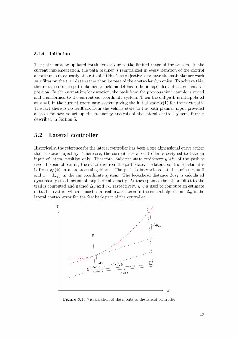
Historically, the reference for the lateral controller has been a one dimensional curve ratherthan a state trajectory. Therefore, the current lateral controller is designed to take aninput of lateral position only. Therefore, only the state trajectory yP (k) of the path isused. Instead of reading the curvature from the path state, the lateral controller estimatesit from yP (k) in a preprocessing block. The path is interpolated at the points x = 0and x = Leff in the car coordinate system. The lookahead distance Leff is calculateddynamically as a function of longitudinal velocity. At these points, the lateral offset to thetrail is computed and named ∆y and yL2 respectively. yL2 is used to compute an estimateof trail curvature which is used as a feedforward term in the control algorithm. ∆y is thelateral control error for the feedback part of the controller.

X

Y

x

y

∆y

Leff

∆yL2

∆Ψ

Figure 3.3: Visualization of the inputs to the lateral controller

19

4Simulation of the lateral control system

Several simulation environments of varying levels of complexity are currently in use inthe autonomous functionality development group. Relatively simple and limited modelsare used for development and tuning and complex high dynamic models are used for ver-ification to minimize the amount of necessary physical testing. Normally, a simulationenvironment is built in Simulink, from blocks of code from the current vehicle imple-mentation, and a vehicle model of varying complexity, depending on the purpose of theenvironment.

For the simulation part of this thesis work, the goal was to produce an environment wherethe lateral behaviour of a vehicle model could be analysed in a situation where the usercould freely specify a drivable area trail to enable isolated analysis of the lateral controlsystem.

It was decided early on that the only feasible way to produce such a simulation environ-ment in the time available was to branch off from a similar, existing environment. Anenvironment designed for development of collision avoidance path generation was chosen.It contained the full lateral control system as well as a relatively simple vehicle modeldescribed in Section 4.1. The trail input to the path planner was generated by higherlevel systems and the user input was of a traffic situation. The work of adapting theenvironment to our purposes consisted of cutting out the higher level system and enableinput of a user generated drivable area trail.

4.1 Vehicle model in simulation environment

The lateral controller group has developed a bicycle model similar to that of [15] describingthe lateral movement of the prototype vehicle at a constant longitudinal speed. The vehiclemodel inputs δwheel and outputs ∆y, the lateral offset from the path, ∆Ψ, the yaw angle

20

error with respect to the path, yL2, the lateral offset at the look ahead distance Leff andΨ, the yawrate of the vehicle with respect to the path. The outputs are chosen as relevantinputs for the lateral controller.

In addition to the vehicle model there is a separate model for the the steering actuator.The steering actuator is a feedback system in itself and thus inputs requested steeringangle δwheel,des and outputs the actual steering angle δwheel.

4.2 Implementation

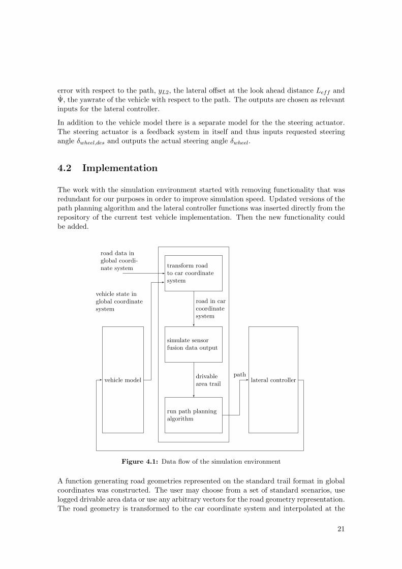
The work with the simulation environment started with removing functionality that wasredundant for our purposes in order to improve simulation speed. Updated versions of thepath planning algorithm and the lateral controller functions was inserted directly from therepository of the current test vehicle implementation. Then the new functionality couldbe added.

vehicle model lateral controller

transform roadto car coordinatesystem

simulate sensorfusion data output

run path planningalgorithm

road data inglobal coordi-nate system

road in carcoordinatesystem

drivablearea trail

path

vehicle state inglobal coordinatesystem

Figure 4.1: Data flow of the simulation environment

A function generating road geometries represented on the standard trail format in globalcoordinates was constructed. The user may choose from a set of standard scenarios, uselogged drivable area data or use any arbitrary vectors for the road geometry representation.The road geometry is transformed to the car coordinate system and interpolated at the

21

points of the regular drivable area x-vector. The result is a road representation on theproper drivable area trail format which can be input to the path planning algorithm. Thedata flow of the simulation environment is illustrated in Figure 4.1.

4.3 Validation

Since the simulation environment was derived from a previous environment that had gonethrough an extensive verification process, and had been used in development in the past,it was decided that verifying conformity with another simulation model was sufficient forour purposes.

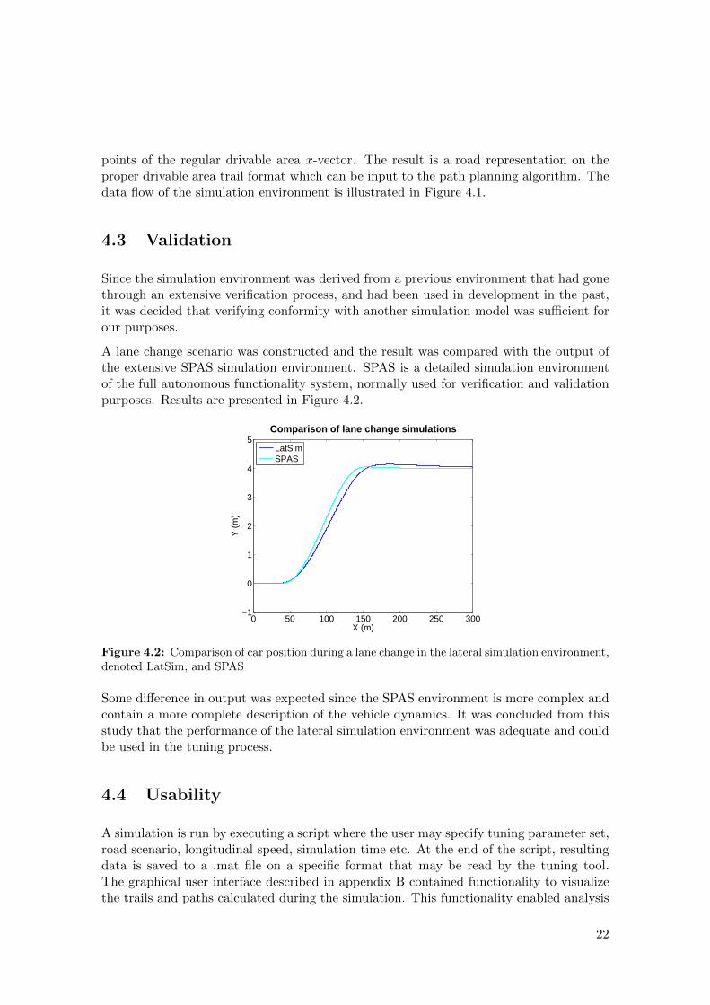
A lane change scenario was constructed and the result was compared with the output ofthe extensive SPAS simulation environment. SPAS is a detailed simulation environmentof the full autonomous functionality system, normally used for verification and validationpurposes. Results are presented in Figure 4.2.

0 50 100 150 200 250 300−1

0

1

2

3

4

5Comparison of lane change simulations

X (m)

Y (

m)

LatSimSPAS

Figure 4.2: Comparison of car position during a lane change in the lateral simulation environment,denoted LatSim, and SPAS

Some difference in output was expected since the SPAS environment is more complex andcontain a more complete description of the vehicle dynamics. It was concluded from thisstudy that the performance of the lateral simulation environment was adequate and couldbe used in the tuning process.

4.4 Usability

A simulation is run by executing a script where the user may specify tuning parameter set,road scenario, longitudinal speed, simulation time etc. At the end of the script, resultingdata is saved to a .mat file on a specific format that may be read by the tuning tool.The graphical user interface described in appendix B contained functionality to visualizethe trails and paths calculated during the simulation. This functionality enabled analysis

22

of path properties as well as momentary ride quality for the simulation. Also, it provedvaluable in the process of debugging the simulation environment implementation.

To enable analysis of how evaluation quantities varied as a function of a tuning parameter,several scripts were built were the simulation run command was executed in a loop. Thesebatch simulation were very efficient in evaluating the impact of tuning parameters on ridequality measures.

23

5Frequency domain analysis

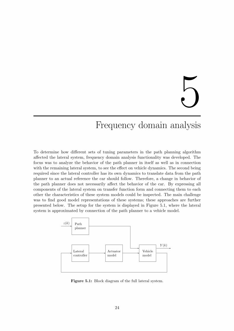
To determine how different sets of tuning parameters in the path planning algorithmaffected the lateral system, frequency domain analysis functionality was developed. Thefocus was to analyze the behavior of the path planner in itself as well as in connectionwith the remaining lateral system, to see the effect on vehicle dynamics. The second beingrequired since the lateral controller has its own dynamics to translate data from the pathplanner to an actual reference the car should follow. Therefore, a change in behavior ofthe path planner does not necessarily affect the behavior of the car. By expressing allcomponents of the lateral system on transfer function form and connecting them to eachother the characteristics of these system models could be inspected. The main challengewas to find good model representations of these systems; these approaches are furtherpresented below. The setup for the system is displayed in Figure 5.1, where the lateralsystem is approximated by connection of the path planner to a vehicle model.

Pathplanner

z(k)

Lateralcontroller

Actuatormodel

Vehiclemodel

Y (k)

Figure 5.1: Block diagram of the full lateral system.

24

5.1 Approximating the path planning algorithm

The path planning algorithm uses a Linear Quadratic Tracking controller, LQT, as de-scribed in Section 3.1. The LQT controller makes use of the full trail vector when con-structing the path. Therefore, there is a transfer function from each element z(k +N) inthe trail, to each element x(k) in the path, where k+N denotes an element further awayon the trail according to N ∈

[0 (kf − k)

].

However, the model of the lateral controller used in this thesis only acts on the first elementin the path, as further explained in Section 5.2.1. Therefore, only the model of the firstoutput of the path planner is required. Moreover, it would be desirable to only use oneinput - this way the path planning algorithm is on a comprehensible form and easy toanalyze. This approximation can be done if it is verified that it captures the dynamics ofthe complete path planning algorithm. Two different approximations for the path planningalgorithm were implemented and compared, one as a simplification of the LQT controllerand one as approximating the LQT controller as a linear quadratic regulator, LQR.

5.1.1 Reduced LQT

The path planning algorithm is a multivariable system of transfer functions, where all ofthem influence the final path. Since a single-input-single-output (SISO) model was desired,the question arose whether simply picking one of the transfer functions to represent thecomplete system would yield a satisfying approximation. By inspecting how differentelements in the trail influenced an element in the path differently, in other words comparinghow z(k + N) and z(k) influenced x(k) differently, a decision could be made on whichtransfer function to choose and analyze if that was good enough.

Putting the expressions for the states and co-states presented in (3.7) and (3.1.3) on acombined state space form yields[

g(k)x(k + 1)

]=

[Mg(k) 0BLg(k) A−BL(k)

] [g(k + 1)x(k)

]+

[W0

]z(k),

which will give the transfer function from z(k) to x(k). By further expanding the expres-sion for g(k),

g(k) = Mg(k)g(k + 1) +Wzk

= Mg(k)(Mg(k + 1)g(k + 2) +Wz(k + 1)) +Wz(k)

= Mg(k)(Mg(k + 1)(Mg(k + 2)g(k + 3) +Wz(k + 2)) +Wz(k + 1)) +Wz(k)

= ...

= (

N∏i=0

Mg(k + i))g(k +N + 1) + (

N−1∑j=0

(

j∏m=0

Mg(k +m))Wz(k +m+ 1)) +Wz(k),

and inserting it into the expression for x(k) it is possible to find the transfer function fromz(k+N) to x(k). Prior to this the matrices L(k),Lg(k) and Mg(k) need to be determined.

25

They are time varying and are solved by looping through the Riccati equation for P, asdescribed in (3.6) and (3.8).

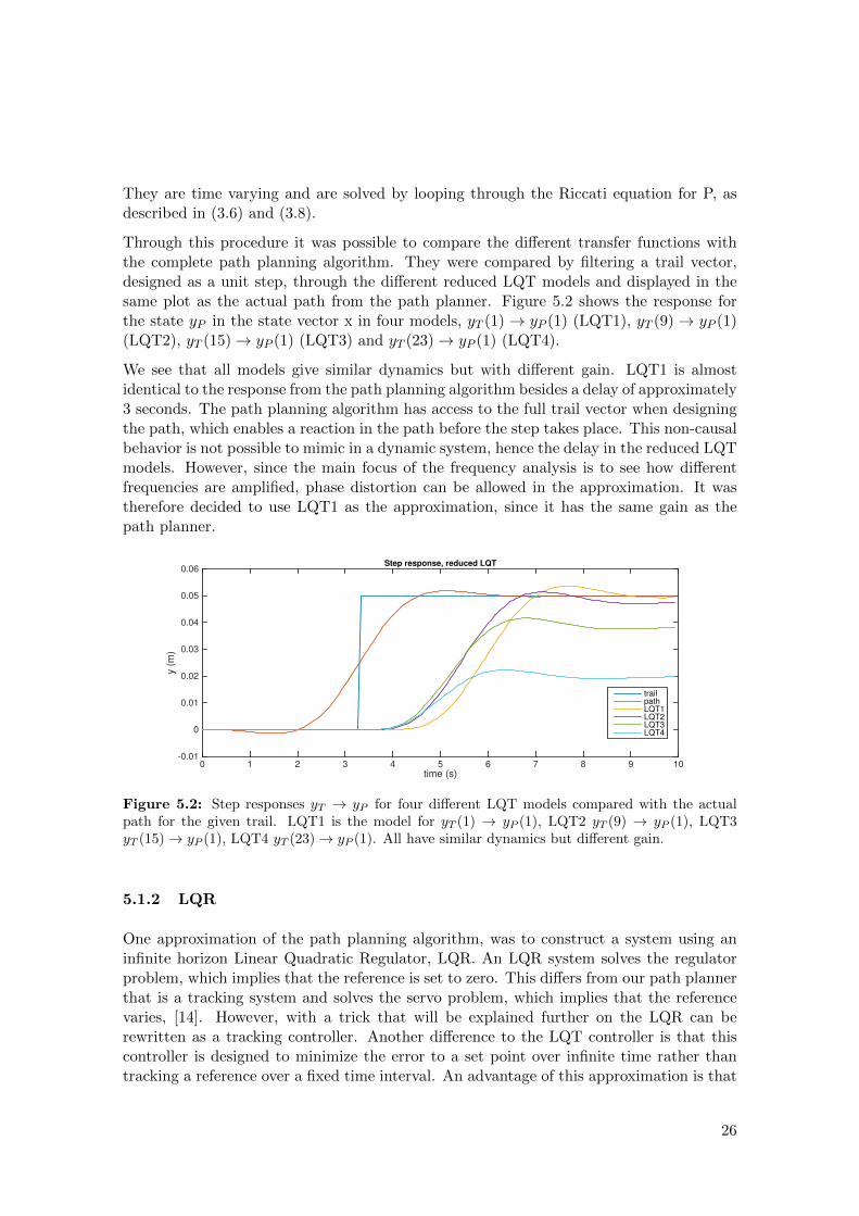
Through this procedure it was possible to compare the different transfer functions withthe complete path planning algorithm. They were compared by filtering a trail vector,designed as a unit step, through the different reduced LQT models and displayed in thesame plot as the actual path from the path planner. Figure 5.2 shows the response forthe state yP in the state vector x in four models, yT (1)→ yP (1) (LQT1), yT (9)→ yP (1)(LQT2), yT (15)→ yP (1) (LQT3) and yT (23)→ yP (1) (LQT4).

We see that all models give similar dynamics but with different gain. LQT1 is almostidentical to the response from the path planning algorithm besides a delay of approximately3 seconds. The path planning algorithm has access to the full trail vector when designingthe path, which enables a reaction in the path before the step takes place. This non-causalbehavior is not possible to mimic in a dynamic system, hence the delay in the reduced LQTmodels. However, since the main focus of the frequency analysis is to see how differentfrequencies are amplified, phase distortion can be allowed in the approximation. It wastherefore decided to use LQT1 as the approximation, since it has the same gain as thepath planner.

time (s)0 1 2 3 4 5 6 7 8 9 10

y (

m)

-0.01

0

0.01

0.02

0.03

0.04

0.05

0.06Step response, reduced LQT

trailpathLQT1LQT2LQT3LQT4

Figure 5.2: Step responses yT → yP for four different LQT models compared with the actualpath for the given trail. LQT1 is the model for yT (1) → yP (1), LQT2 yT (9) → yP (1), LQT3yT (15)→ yP (1), LQT4 yT (23)→ yP (1). All have similar dynamics but different gain.

5.1.2 LQR

One approximation of the path planning algorithm, was to construct a system using aninfinite horizon Linear Quadratic Regulator, LQR. An LQR system solves the regulatorproblem, which implies that the reference is set to zero. This differs from our path plannerthat is a tracking system and solves the servo problem, which implies that the referencevaries, [14]. However, with a trick that will be explained further on the LQR can berewritten as a tracking controller. Another difference to the LQT controller is that thiscontroller is designed to minimize the error to a set point over infinite time rather thantracking a reference over a fixed time interval. An advantage of this approximation is that

26

the feedback gain of the controller is time independent, resulting in a much simpler systemthan for the original path planning algorithm, where we have transfer functions from allelements in the reference to all elements in the path.

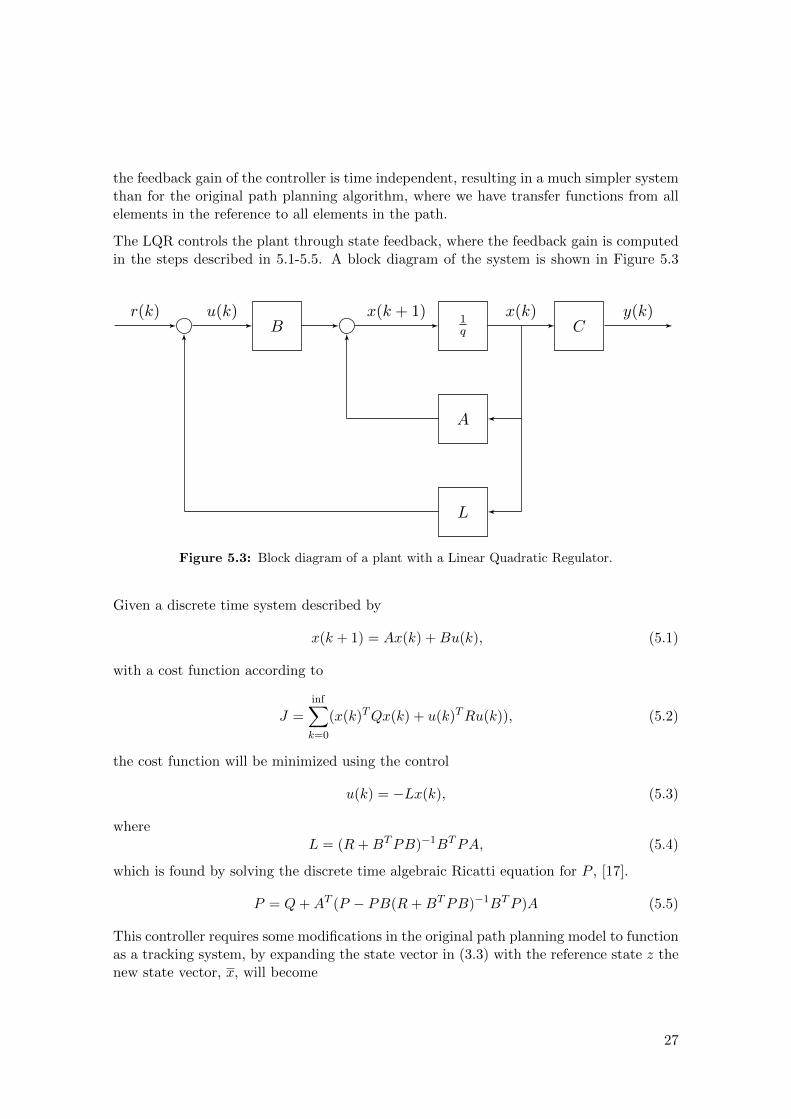
The LQR controls the plant through state feedback, where the feedback gain is computedin the steps described in 5.1-5.5. A block diagram of the system is shown in Figure 5.3

r(k)B

u(k)1q

x(k + 1)C

x(k) y(k)

A

L

Figure 5.3: Block diagram of a plant with a Linear Quadratic Regulator.

Given a discrete time system described by

x(k + 1) = Ax(k) +Bu(k), (5.1)

with a cost function according to

J =inf∑k=0

(x(k)TQx(k) + u(k)TRu(k)), (5.2)

the cost function will be minimized using the control

u(k) = −Lx(k), (5.3)

whereL = (R+BTPB)−1BTPA, (5.4)

which is found by solving the discrete time algebraic Ricatti equation for P , [17].

P = Q+AT (P − PB(R+BTPB)−1BTP )A (5.5)

This controller requires some modifications in the original path planning model to functionas a tracking system, by expanding the state vector in (3.3) with the reference state z thenew state vector, x, will become

27

x =

[x(k)z(k)

]=

yP (k)ΨP (k)

ΨP (k)yT (k)ΨT (k)

ΨT (k)

.

The reference r is now incorporated into the state vector, set as constant. It will berewritten as an input later on.

With this new state vector the full model can be written as

x(k + 1) = Ax(k) +Bu,

y = Cx(k),

where

A =

[A 00 I

], B =

[B0

], C =

[I 0

],

and the A and B matrices are the discretized versions of the matrices presented in (3.4).The LQ feedback gain L =

[Lx Lz

]forms the feedback u(k) = −Lx(k) which generates

the closed loop system according to

x(k + 1) = Ax(k) +Bu

= (A−BL)x(k).

The closed loop system then becomes[x(k + 1)z(k + 1)

]=

[[A 00 I

]−[BLx BLz

0 0

]] [x(k)z(k)

],

where the first row, x(k), is described as

x(k + 1) =[A−BLx

]x(k)−BLzz(k).

This equation can in itself be interpreted as a state space representation where z(k) is theinput to the system. Setting the states x(k) as outputs we get the system

x(k + 1) =[A−BLx

]x(k)−

[BLz

]z(k),

y = Ix(k),

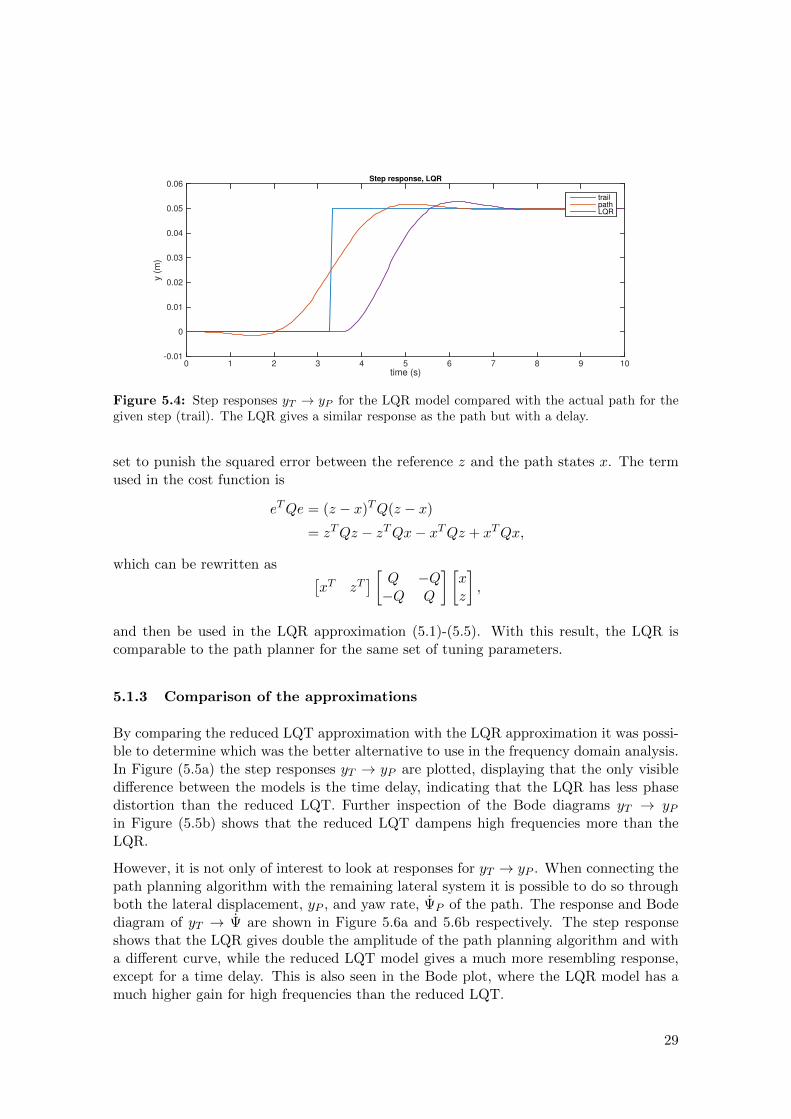
which is the LQR approximation of the path planning algorithm. The step response forthe approximation is presented in Figure 5.4. It is seen that the LQR approximation givessimilar response as the path planning algorithm, but with a time delay, similarly to thereduced LQT approximation.

Even though the LQR approximation has an extended state vector the same tuning pa-rameters could be used as for the path planner. The path planner’s tuning matrix Q is

28

time (s)0 1 2 3 4 5 6 7 8 9 10

y (

m)

-0.01

0

0.01

0.02

0.03

0.04

0.05

0.06Step response, LQR

trailpathLQR

Figure 5.4: Step responses yT → yP for the LQR model compared with the actual path for thegiven step (trail). The LQR gives a similar response as the path but with a delay.

set to punish the squared error between the reference z and the path states x. The termused in the cost function is

eTQe = (z − x)TQ(z − x)

= zTQz − zTQx− xTQz + xTQx,

which can be rewritten as [xT zT

] [ Q −Q−Q Q

] [xz

],

and then be used in the LQR approximation (5.1)-(5.5). With this result, the LQR iscomparable to the path planner for the same set of tuning parameters.

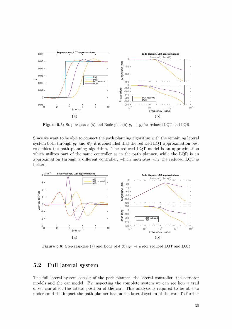
5.1.3 Comparison of the approximations

By comparing the reduced LQT approximation with the LQR approximation it was possi-ble to determine which was the better alternative to use in the frequency domain analysis.In Figure (5.5a) the step responses yT → yP are plotted, displaying that the only visibledifference between the models is the time delay, indicating that the LQR has less phasedistortion than the reduced LQT. Further inspection of the Bode diagrams yT → yPin Figure (5.5b) shows that the reduced LQT dampens high frequencies more than theLQR.

However, it is not only of interest to look at responses for yT → yP . When connecting thepath planning algorithm with the remaining lateral system it is possible to do so throughboth the lateral displacement, yP , and yaw rate, ΨP of the path. The response and Bodediagram of yT → Ψ are shown in Figure 5.6a and 5.6b respectively. The step responseshows that the LQR gives double the amplitude of the path planning algorithm and witha different curve, while the reduced LQT model gives a much more resembling response,except for a time delay. This is also seen in the Bode plot, where the LQR model has amuch higher gain for high frequencies than the reduced LQT.

29

time (s)0 2 4 6 8 10

y

-0.01

0

0.01

0.02

0.03

0.04

0.05

0.06Step response, LQT approximations

trailpathLQT reducedLQR

(a)

Magnitude (

dB

)

-150

-100

-50

0From: z(1) To: x(1)

10-1

100

101

102

Phase (

deg)

-1080

-900

-720

-540

-360

-180

0

LQT reducedLQR

Bode diagram, LQT approximations

Frequency (rad/s)

(b)

Figure 5.5: Step response (a) and Bode plot (b) yT → yP for reduced LQT and LQR

Since we want to be able to connect the path planning algorithm with the remaining lateralsystem both through yP and ΨP it is concluded that the reduced LQT approximation bestresembles the path planning algorithm. The reduced LQT model is an approximationwhich utilizes part of the same controller as in the path planner, while the LQR is anapproximation through a different controller, which motivates why the reduced LQT isbetter.

time (s)0 2 4 6 8 10

yaw

rate

(dΨ

/dt)

×10-3

-3

-2

-1

0

1

2

3

4Step response, LQT approximations

pathLQT reducedLQR

(a)

Magnitude (

dB

)

-120

-100

-80

-60

-40

-20

0From: z(1) To: x(3)

10-2

10-1

100

101

102

Phase (

deg)

-720

-540

-360

-180

0

180

LQT reducedLQR

Bode diagram, LQT approxaimtions

Frequency (rad/s)

(b)

Figure 5.6: Step response (a) and Bode plot (b) yT → ΨP for reduced LQT and LQR

5.2 Full lateral system

The full lateral system consist of the path planner, the lateral controller, the actuatormodels and the car model. By inspecting the complete system we can see how a trailoffset can affect the lateral position of the car. This analysis is required to be able tounderstand the impact the path planner has on the lateral system of the car. To further

30

elaborate, the path planner generates a reference to the lateral controller, but since thelateral controller has its own dynamics the given path might be deviated from.

5.2.1 Lateral controller, actuators and car model

In the lateral control system in the car the controller is designed to control on data fromtwo points in the path, the first element and an element further away on the path, calledthe look-ahead point. The model used in the frequency domain analysis functions slightlydifferent. Instead of feeding the controller with path data, the car model is perturbed byeither a yaw rate or a lateral offset, when put in closed loop with the lateral controllerand actuator model the controller will work as to follow the perturbation. This yields agood approximation of the lateral control system implemented in the car. The transferfunctions for the closed loop system were derived by the lateral control group at Volvo withoutputs ∆y,∆Ψ, yL2, Ψ and inputs δyinj , Ψinj , further presented in Section 3.2. The inputsenabled two ways of connecting to the path planner, either as a measurement disturbanceon y through ∆yinj or as a disturbance on the desired yaw rate through Ψinj .

By adding a coordinate transformation after the car model the state global lateral positioncould be computed according to (5.6). This model is however limited to only work forsmall angles Ψ, the consequence is that it is only possible to perform a frequency domainanalysis for small or no perturbation in the curvature of the trail.

Ψ(k + 1) = Ψ(k) + dt ∗ Ψ(k),

Y (k + 1) = Y (k) + dt(y cos Ψ + vx sin Ψ)

≈ Y (k) + dt(y + vxΨ).

(5.6)

5.2.2 Connecting the path planner to the remaining lateral system

There were two different ways of connecting the path planner to the remaining lateralsystem, as a disturbance on Ψ, which is the desired yaw rate of the path, or through ∆ywhich is a measurement disturbance on lateral offset, further shown in Figure 5.7.

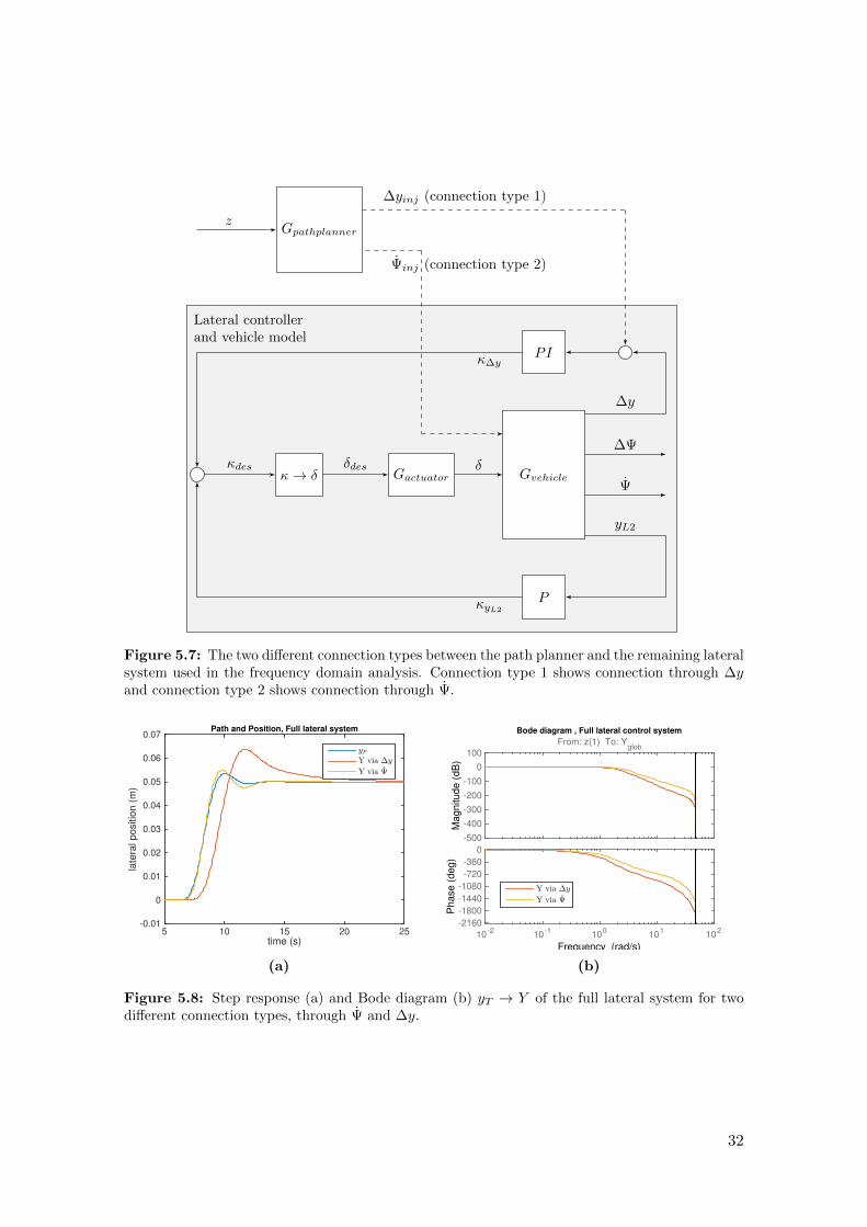
These two different systems were both developed and compared, their Bode diagrams canbe viewed in Figure 5.8b. It is seen that connecting through ∆y results in a lower cut offfrequency and more phase distortion for high frequencies. By inspection of simulated timeresponses for the two connection types that are put in comparison with the path, Figure5.8a, one can reason which type best resembles the actual system. According to the groupdeveloping the lateral controller it is designed to follow the path in an almost identicalmanner, as long as the path does not generate too fast lateral displacement. Connectingthrough Ψ yields an almost identical response in lateral position of the car as the path.Connecting through ∆y gives a response that does not follow the path as well, it is bothslower and has a larger overshoot. Therefore, it was concluded that connecting throughΨ should give a model best resembling the actual system.

31

Lateral controllerand vehicle model

κ→ δ Gactuator Gvehicle

PI

P

δdes δ

∆y

∆Ψ

Ψ

yL2

κdes

κyL2

Gpathplanner

Ψinj (connection type 2)

κ∆y

∆yinj (connection type 1)

z

Figure 5.7: The two different connection types between the path planner and the remaining lateralsystem used in the frequency domain analysis. Connection type 1 shows connection through ∆yand connection type 2 shows connection through Ψ.

time (s)5 10 15 20 25

late

ral positio

n (

m)

-0.01

0

0.01

0.02

0.03

0.04

0.05

0.06

0.07Path and Position, Full lateral system

yPY via ∆y

Y via Ψ

(a)

Magnitude (

dB

)

-500

-400

-300

-200

-100

0

100

From: z(1) To: Yglob

10-2

10-1

100

101

102

Phase (

deg)

-2160

-1800

-1440

-1080

-720

-360

0

Y via ∆y

Y via Ψ

Bode diagram , Full lateral control system

Frequency (rad/s)

(b)

Figure 5.8: Step response (a) and Bode diagram (b) yT → Y of the full lateral system for twodifferent connection types, through Ψ and ∆y.

32

5.3 Validation

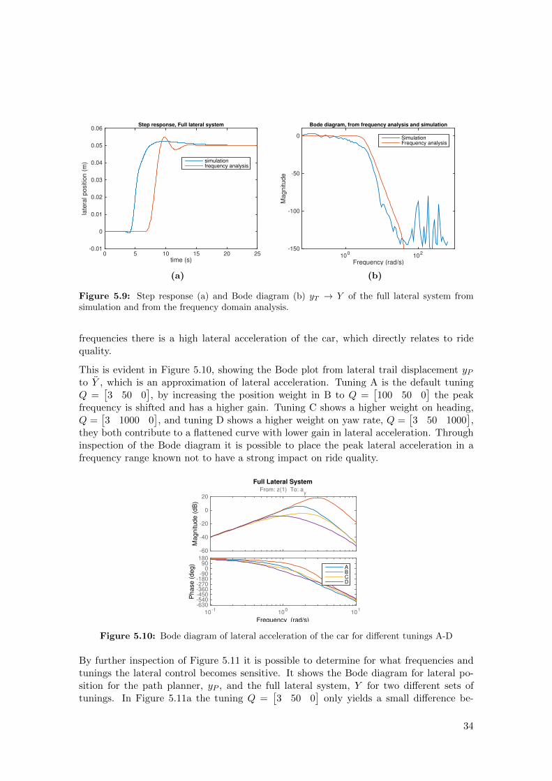
The models of the path planner and the full lateral system needed to be validated beforeusing the results of the frequency domain analysis. The path planner is already validatedin Section 5.1.3 where the model of the chosen approximation is compared with the actualpath planner, with the conclusion that it is a satisfying approximation. The performanceof the model of the complete lateral system could not be determined in a similar mannerbut was instead compared to the results of the simulation environment. When looking at asimulated step response in Figure 5.9a it is evident that the simulation environment givesdifferent results than the frequency domain analysis. The frequency analysis model givesslightly higher overshoot and an oscillating behavior which the simulation environmentdoes not yield, it is in other words more sensitive. Also, it has a time delay, a result ofthe approximation of the path planner, which has already been discussed in Section 5.1.1and can be disregarded.

They both share similar characteristics of the path planner, therefore it must be thelateral controller models that differs. The simulation environment has a less aggressiveimplementation of the lateral controller which results in a smoother response. In thefrequency domain analysis the model of the lateral controller is linear, but the actuallateral controller contains non-linearities. These non-linearities are rate constraints andsaturations and they are present in the simulation environment. They are used to preventa rapid response when the path is considered aggressive. Therefore only a small step of 5cm was simulated, so that these effects should not occur. It might still be that the smoothappearance of the step from the simulation can be explained by the non-linearities.

Through excitation of the simulation model an approximative magnitude response of thesimulation environment could be found. This was achieved by taking the fast Fouriertransform (FFT) of a simulated sine curve and then saving the magnitude for the frequencyof the given curve. This was done for a range of frequencies that could be assembled intoa magnitude response. When comparing it to that of the frequency analysis, in Figure5.9b, more similarities between the two representations are disclosed. Even though thecut-off frequencies differ, they share the same overall appearance and steepness of thecurves. That the model from the frequency analysis is more sensitive than the simulationmodel can also be seen in the magnitude response, where the gain is higher for highfrequencies. It is important to realize that the magnitude response of the simulation is onlyan approximation, taking the FFT does not give a perfect spectrum, so the main conclusionof this analysis should be that the magnitude responses show the same tendencies. Furtheruse of the models found in this chapter for tuning of the path planner was believed to bemeaningful.

5.4 Usability

The frequency domain analysis was developed to display information of the effects differenttunings have on system characteristics. It shows how different frequencies are distortedin phase and gain. The main feature of the analysis is the possibility to see for which

33

time (s)0 5 10 15 20 25

late

ral positio

n (

m)

-0.01

0

0.01

0.02

0.03

0.04

0.05

0.06Step response, Full lateral system

simulationfrequency analysis

(a)

Frequency (rad/s)10

010

2

Magnitude

-150

-100

-50

0

Bode diagram, from frequency analysis and simulation

SimulationFrequency analysis

(b)

Figure 5.9: Step response (a) and Bode diagram (b) yT → Y of the full lateral system fromsimulation and from the frequency domain analysis.

frequencies there is a high lateral acceleration of the car, which directly relates to ridequality.

This is evident in Figure 5.10, showing the Bode plot from lateral trail displacement yPto Y , which is an approximation of lateral acceleration. Tuning A is the default tuningQ =

[3 50 0

], by increasing the position weight in B to Q =

[100 50 0

]the peak

frequency is shifted and has a higher gain. Tuning C shows a higher weight on heading,Q =

[3 1000 0

], and tuning D shows a higher weight on yaw rate, Q =

[3 50 1000

],

they both contribute to a flattened curve with lower gain in lateral acceleration. Throughinspection of the Bode diagram it is possible to place the peak lateral acceleration in afrequency range known not to have a strong impact on ride quality.

Magnitude (

dB

)

-60

-40

-20

0

20

From: z(1) To: ay

10-1

100

101

Phase (

deg)

-630-540-450-360-270-180

-900

90180

ABCD

Full Lateral System

Frequency (rad/s)

Figure 5.10: Bode diagram of lateral acceleration of the car for different tunings A-D

By further inspection of Figure 5.11 it is possible to determine for what frequencies andtunings the lateral control becomes sensitive. It shows the Bode diagram for lateral po-sition for the path planner, yP , and the full lateral system, Y for two different sets oftunings. In Figure 5.11a the tuning Q =

[3 50 0

]only yields a small difference be-

34

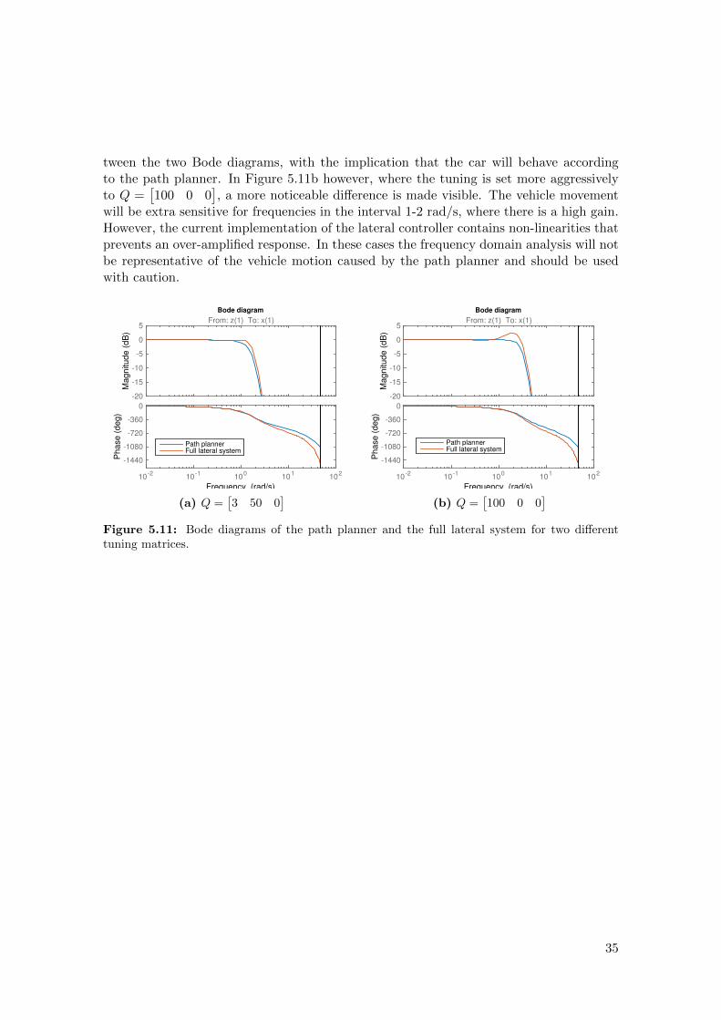
tween the two Bode diagrams, with the implication that the car will behave accordingto the path planner. In Figure 5.11b however, where the tuning is set more aggressivelyto Q =

[100 0 0

], a more noticeable difference is made visible. The vehicle movement

will be extra sensitive for frequencies in the interval 1-2 rad/s, where there is a high gain.However, the current implementation of the lateral controller contains non-linearities thatprevents an over-amplified response. In these cases the frequency domain analysis will notbe representative of the vehicle motion caused by the path planner and should be usedwith caution.

Magnitude (

dB

)

-20

-15

-10

-5

0

5From: z(1) To: x(1)

10-2

10-1

100

101

102

Phase (

deg)

-1440

-1080

-720

-360

0

Path plannerFull lateral system

Bode diagram

Frequency (rad/s)

(a) Q =[3 50 0

]

Magnitude (

dB

)

-20

-15

-10

-5

0

5From: z(1) To: x(1)

10-2

10-1

100

101

102

Phase (

deg)

-1440

-1080

-720

-360

0

Path plannerFull lateral system

Bode diagram

Frequency (rad/s)

(b) Q =[100 0 0

]Figure 5.11: Bode diagrams of the path planner and the full lateral system for two differenttuning matrices.

35

6Experiments and results

The experiments were designed to evaluate whether ride quality could be improved bytuning the path planning algorithm, using the tools developed during the project. Thefirst experiment investigated whether the ride quality measures could differentiate be-tween manual and autonomous driving. The subsequent experiments dealt with tuningof the path planning algorithm by use of the new tools, with the aim to improve ridequality.

Test sessions were conducted in one of the prototype autonomous V60s in service at VolvoResearch and development at Torslanda. The test vehicle was equipped with extensivelogging equipment to enable software replay of test runs. Our tests took place on Lund-byleden, which is a stretch of commuter road encircling Goteborg where Volvo aims tointroduce autonomous functionality in the near future.

6.1 Comparing manual and autonomous driving

To evaluate the ride quality performance of the current implementation of the AD car ona straight road an experiment was designed where the car was driven in AD-mode alonga specific road section while lateral acceleration was logged. Thereafter, the same sectionwas driven and logged in manual mode. The ride quality evaluation methods were appliedto the two measurements, to decide if there was a difference in estimated ride quality. Theexperiment yielded the following results.

The spectral content of the two measurement series was examined from the accelerationspectrum in Figure 6.1.

36

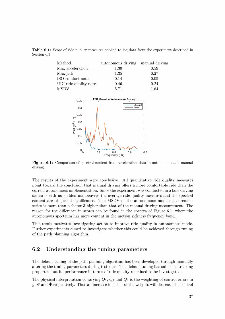
Table 6.1: Score of ride quality measures applied to log data from the experiment described inSection 6.1

Method autonomous driving manual driving

Max acceleration 1.30 0.59Max jerk 1.35 0.27ISO comfort note 0.14 0.05UIC ride quality note 0.46 0.24MSDV 5.71 1.64

Frequency (Hz)0 0.2 0.4 0.6 0.8

PS

D (

G2/H

z)

0

0.05

0.1

0.15

0.2

0.25

0.3

0.35PSD Manual vs Autonomous Driving

ManualAuto

Figure 6.1: Comparison of spectral content from acceleration data in autonomous and manualdriving

The results of the experiment were conclusive. All quantitative ride quality measurespoint toward the conclusion that manual driving offers a more comfortable ride than thecurrent autonomous implementation. Since the experiment was conducted in a lane drivingscenario with no sudden manoeuvres the average ride quality measures and the spectralcontent are of special significance. The MSDV of the autonomous mode measurementseries is more than a factor 3 higher than that of the manual driving measurement. Thereason for the difference in scores can be found in the spectra of Figure 6.1, where theautonomous spectrum has more content in the motion sickness frequency band.

This result motivates investigating action to improve ride quality in autonomous mode.Further experiments aimed to investigate whether this could be achieved through tuningof the path planning algorithm.

6.2 Understanding the tuning parameters

The default tuning of the path planning algorithm has been developed through manuallyaltering the tuning parameters during test runs. The default tuning has sufficient trackingproperties but its performance in terms of ride quality remained to be investigated.

The physical interpretation of varying Q1, Q2 and Q3 is the weighting of control errors iny, Ψ and Ψ respectively. Thus an increase in either of the weights will decrease the control

37

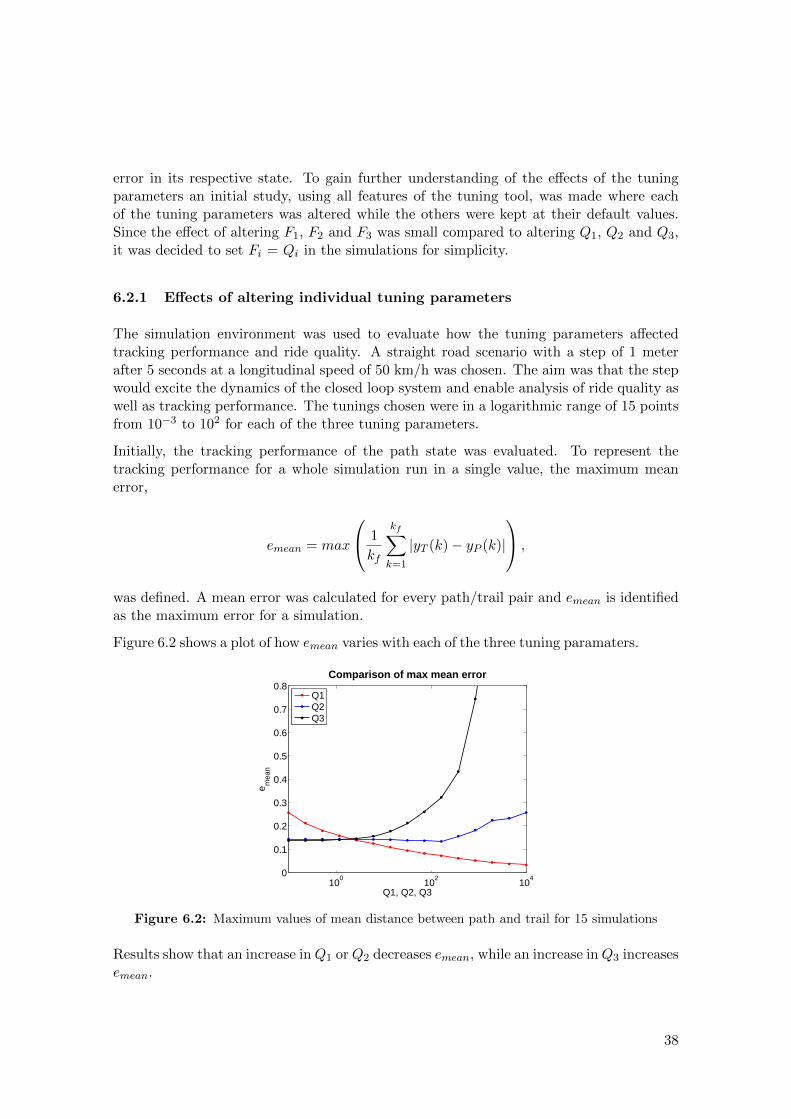
error in its respective state. To gain further understanding of the effects of the tuningparameters an initial study, using all features of the tuning tool, was made where eachof the tuning parameters was altered while the others were kept at their default values.Since the effect of altering F1, F2 and F3 was small compared to altering Q1, Q2 and Q3,it was decided to set Fi = Qi in the simulations for simplicity.

6.2.1 Effects of altering individual tuning parameters

The simulation environment was used to evaluate how the tuning parameters affectedtracking performance and ride quality. A straight road scenario with a step of 1 meterafter 5 seconds at a longitudinal speed of 50 km/h was chosen. The aim was that the stepwould excite the dynamics of the closed loop system and enable analysis of ride quality aswell as tracking performance. The tunings chosen were in a logarithmic range of 15 pointsfrom 10−3 to 102 for each of the three tuning parameters.

Initially, the tracking performance of the path state was evaluated. To represent thetracking performance for a whole simulation run in a single value, the maximum meanerror,

emean = max

1

kf

kf∑k=1

|yT (k)− yP (k)|

,

was defined. A mean error was calculated for every path/trail pair and emean is identifiedas the maximum error for a simulation.

Figure 6.2 shows a plot of how emean varies with each of the three tuning paramaters.

100

102

104

0

0.1

0.2

0.3

0.4

0.5

0.6

0.7

0.8Comparison of max mean error

Q1, Q2, Q3

e mea

n

Q1Q2Q3

Figure 6.2: Maximum values of mean distance between path and trail for 15 simulations

Results show that an increase inQ1 orQ2 decreases emean, while an increase inQ3 increasesemean.

38

Finally, the ride quality evaluation functionality was used to study the effects of the tuningparameters on ride quality measures for the same simulation scenario.

The ride quality performance of the path state for the batch simulations is displayed inFigure 6.3. Results show that lateral acceleration and jerk increases with increasing Q1

and Q2 but decreases with increasing Q3. This is expected since a decreased controlerror in y or Ψ should lead to a improved tracking performance and more rapid lateralmovement. A decreased control error in Ψ relates to tight following of the road curvaturewhich is 0 for our scenario. Thus, high values of Q3 leads to less rapid lateral movementand poor tracking properties. At approximately Q3 > 103 there is an increase in jerk andacceleration levels that does not conform with the above reasoning. However, closer reviewof these individual simulations reveals that tracking performance in this case is very poorso the relevance of results at these levels of Q3 is low.

The average ride quality measures show similar properties as the acceleration and jerk.

After studying how the path state was affected by the path planner tuning parameters theinvestigation continued with analysis of the vehicle model state for the same simulationscenario.

The current implementation of the lateral controller contains functionality to constrainthe output if the input path is not kinematically feasible. This is evident when comparingmaximum acceleration and jerk levels between the results in Figures 6.3 and 6.4. Thehigh levels of acceleration an jerk for the path state does not propagate out to the vehiclemodel state. An interesting result is that there appears to be local minima in ride qualityat approximately Q1 = 3, Q3 = 0 and Q1 = 3, Q3 = 215. This is seen also in the plots forthe path state but more clearly for the vehicle model state.

6.2.2 Effects of altering multiple tuning parameters

It was noted in Figures 6.2, 6.3 and 6.4 that an increase in Q3 had a positive influenceon ride quality but a negative influence on tracking performance. On the other hand, anincrease in Q1 had a negative influence on ride quality but a positive influence on trackingperformance. Therefore it was decided that a study where both Q1 and Q3 were variedwas worth investigating.

This was done by running the simulation environment in a nested for loop for Q1 =[10−1 103] and Q3 = [10−1 104]. The result for each of the ride quality measures aswell as the maximum mean error was stored in matrices and reviewed in the surface plotsdisplayed in Figure 6.6.

The result unveiled that the default tuning is close to optimal but the minima of ridequality parameters are in the vicinity of Q1 = 101 and Q3 = 103.

A tradeoff between ride quality and tracking performance becomes evident when com-paring the emean plot of Figure 6.5 with the ride quality performance plots. Trackingperformance is poor at low Q1 and high Q3. The tuning [Q1 Q2 Q3] = [6 50 215] waschosen for further evaluation since it had the best ride quality of the points with emean

lower or equal to that of the default tuning.

39

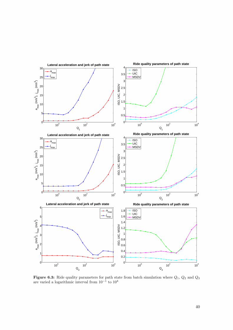
100

102

104

0

5

10

15

20

25

30Lateral acceleration and jerk of path state

Q1

a max

(m

/s2 ),

jm

ax (

m/s

3 )

amax

jmax

100

102

104

0

0.5

1

1.5

2

2.5

3

3.5

4Ride quality parameters of path state

Q1

ISO

, UIC

, MS

DV

ISOUICMSDV

100

102

104

0

5

10

15

20

25

30Lateral acceleration and jerk of path state

Q2

a max

(m

/s2 ),

jm

ax (

m/s

3 )

amax

jmax

100

102

104

0

0.5

1

1.5

2

2.5

3

3.5

4Ride quality parameters of path state

Q2

ISO

, UIC

, MS

DV

ISOUICMSDV

100

102

104

0

1

2

3

4

5

6Lateral acceleration and jerk of path state

Q3

a max

(m

/s2 ),

jm

ax (

m/s

3 )

amax

jmax

100

102

104

0

0.2

0.4

0.6

0.8

1

1.2

1.4

1.6

1.8

Ride quality parameters of path state

Q3

ISO

, UIC

, MS

DV

ISOUICMSDV

Figure 6.3: Ride quality parameters for path state from batch simulation where Q1, Q2 and Q3

are varied a logarithmic interval from 10−1 to 104

40

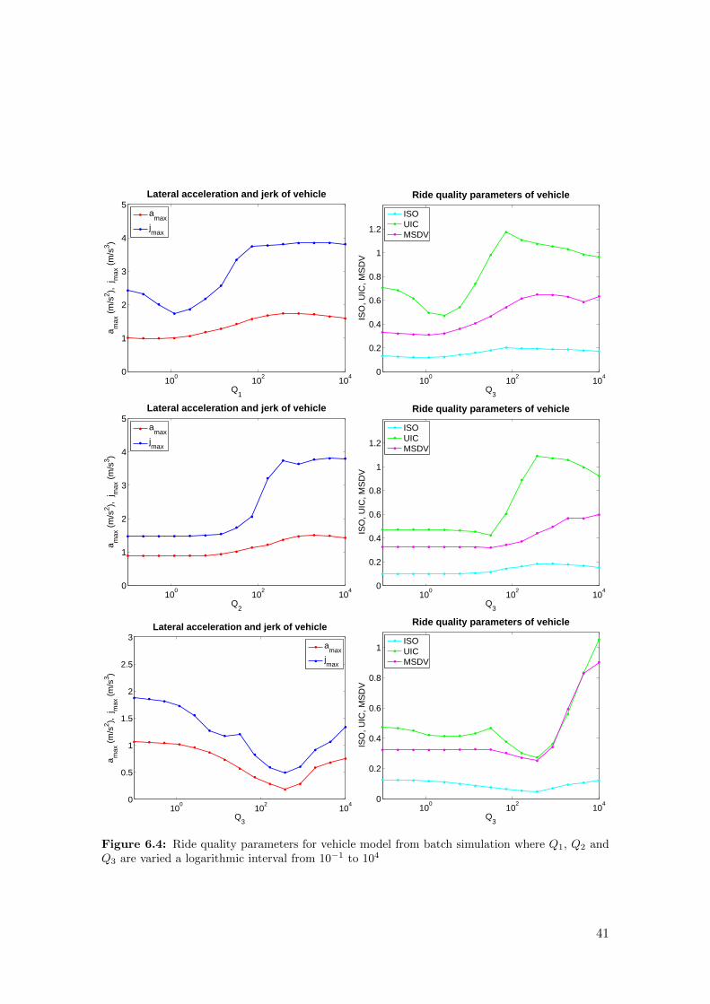
100

102

104

0

1

2

3

4

5Lateral acceleration and jerk of vehicle

Q1

a max

(m

/s2 ),

jm

ax (

m/s

3 )

amax

jmax

100

102

104

0

0.2

0.4

0.6

0.8

1

1.2

Ride quality parameters of vehicle

Q3

ISO

, UIC

, MS

DV

ISOUICMSDV

100

102

104

0

1

2

3

4

5Lateral acceleration and jerk of vehicle

Q2

a max

(m

/s2 ),

jm

ax (

m/s

3 )

amax

jmax

100

102

104

0

0.2

0.4

0.6

0.8

1

1.2

Ride quality parameters of vehicle

Q3

ISO

, UIC

, MS

DV

ISOUICMSDV

100

102

104

0

0.5

1

1.5

2

2.5

3Lateral acceleration and jerk of vehicle

Q3

a max

(m

/s2 ),

jm

ax (

m/s

3 )

amax

jmax

100

102

104

0

0.2

0.4

0.6

0.8

1

Ride quality parameters of vehicle

Q3

ISO

, UIC

, MS

DV

ISOUICMSDV

Figure 6.4: Ride quality parameters for vehicle model from batch simulation where Q1, Q2 andQ3 are varied a logarithmic interval from 10−1 to 104

41

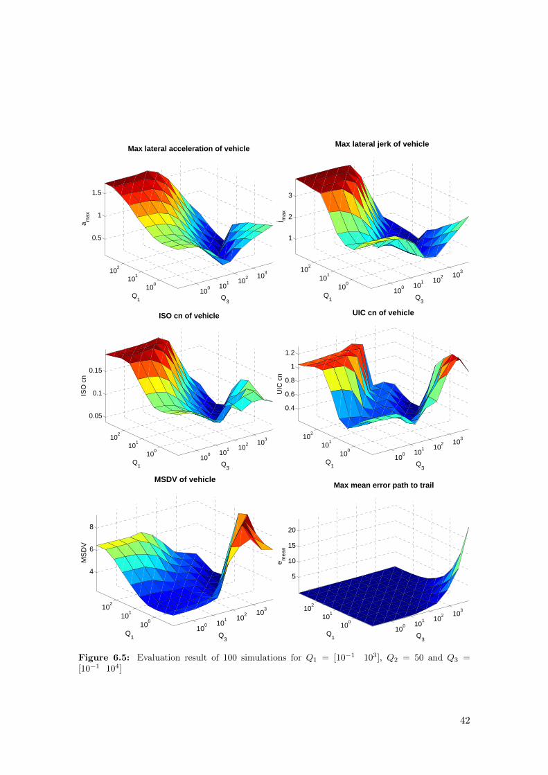
100 10

1 102 10

3

100

101

102

0.5

1

1.5

Q3

Max lateral acceleration of vehicle

Q1

a max

100 10

1 102 10

3

100

101

102

1

2

3

Q3

Max lateral jerk of vehicle

Q1

j max

100 10

1 102 10

3

100

101

102

0.05

0.1

0.15

Q3

ISO cn of vehicle

Q1

ISO

cn

100 10

1 102 10

3

100

101

102

0.4

0.6

0.8

1

1.2

Q3

UIC cn of vehicle

Q1

UIC

cn

100 10

1 102 10

3

100

101

102

4

6

8

Q3

MSDV of vehicle

Q1

MS

DV

100 10

1 102 10

3

100

101

102

5

10

15

20

Q3

Max mean error path to trail

Q1

e mea

n

Figure 6.5: Evaluation result of 100 simulations for Q1 = [10−1 103], Q2 = 50 and Q3 =[10−1 104]

42

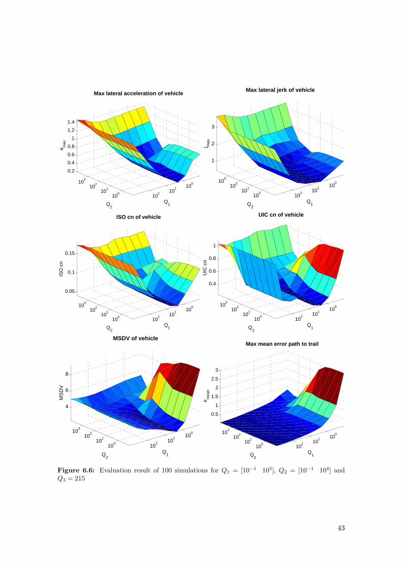
10010

110210

3

100

101

102

0.2

0.4

0.6

0.8

1

1.2

1.4

Q1

Max lateral acceleration of vehicle

Q2

a max

10010

110210

3

100

101

102

1

2

3

Q1

Max lateral jerk of vehicle

Q2

j max

10010

110210

3

100

101

102

0.05

0.1

0.15

Q1

ISO cn of vehicle

Q2

ISO

cn

10010

110210

3

100

101

102

0.4

0.6

0.8

1

Q1

UIC cn of vehicle

Q2

UIC

cn

10010

110210

3

100

101

102

4

6

8

Q1

MSDV of vehicle

Q2

MS

DV

10010

110210

3

100

101

102

0.5

1

1.5

2

2.5

3

Q1

Max mean error path to trail

Q2

e mea

n

Figure 6.6: Evaluation result of 100 simulations for Q1 = [10−1 103], Q2 = [10−1 104] andQ3 = 215

43

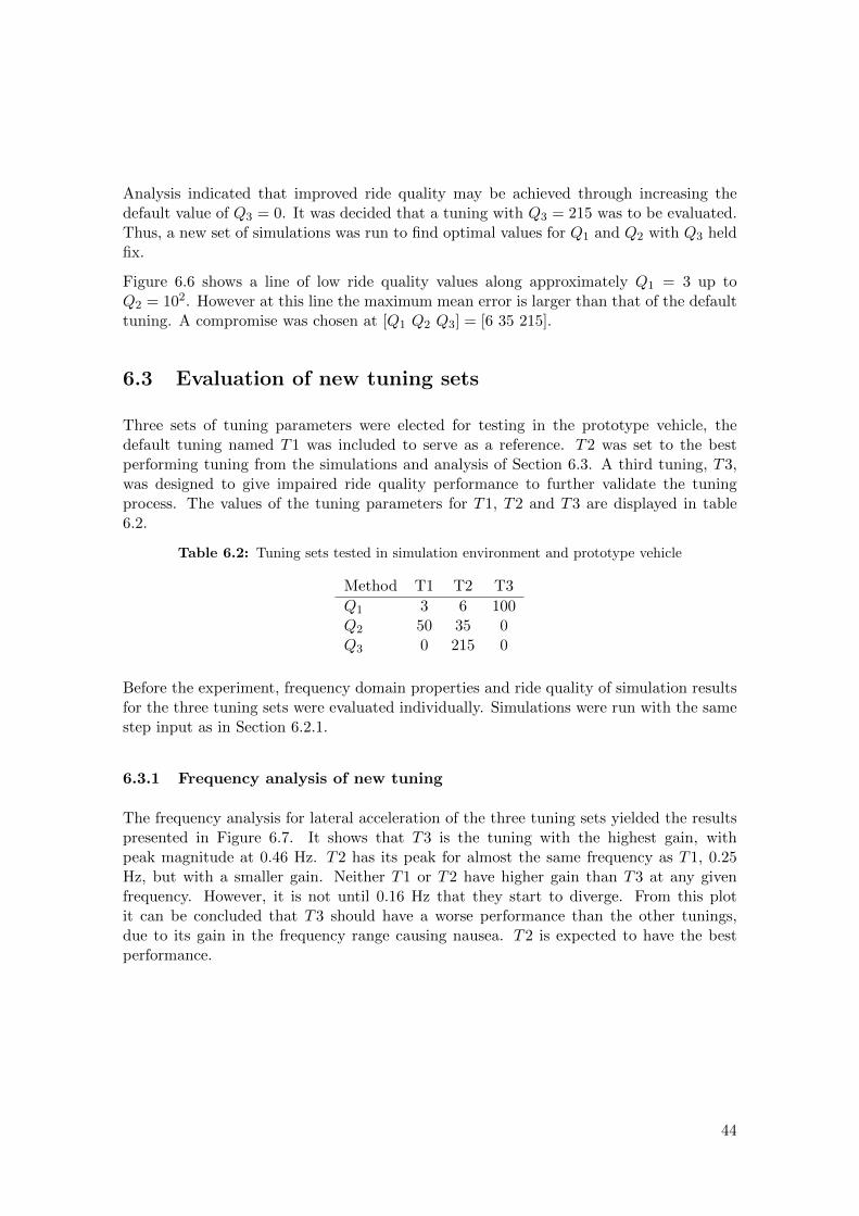
Analysis indicated that improved ride quality may be achieved through increasing thedefault value of Q3 = 0. It was decided that a tuning with Q3 = 215 was to be evaluated.Thus, a new set of simulations was run to find optimal values for Q1 and Q2 with Q3 heldfix.

Figure 6.6 shows a line of low ride quality values along approximately Q1 = 3 up toQ2 = 102. However at this line the maximum mean error is larger than that of the defaulttuning. A compromise was chosen at [Q1 Q2 Q3] = [6 35 215].

6.3 Evaluation of new tuning sets

Three sets of tuning parameters were elected for testing in the prototype vehicle, thedefault tuning named T1 was included to serve as a reference. T2 was set to the bestperforming tuning from the simulations and analysis of Section 6.3. A third tuning, T3,was designed to give impaired ride quality performance to further validate the tuningprocess. The values of the tuning parameters for T1, T2 and T3 are displayed in table6.2.

Table 6.2: Tuning sets tested in simulation environment and prototype vehicle

Method T1 T2 T3

Q1 3 6 100Q2 50 35 0Q3 0 215 0

Before the experiment, frequency domain properties and ride quality of simulation resultsfor the three tuning sets were evaluated individually. Simulations were run with the samestep input as in Section 6.2.1.

6.3.1 Frequency analysis of new tuning

The frequency analysis for lateral acceleration of the three tuning sets yielded the resultspresented in Figure 6.7. It shows that T3 is the tuning with the highest gain, withpeak magnitude at 0.46 Hz. T2 has its peak for almost the same frequency as T1, 0.25Hz, but with a smaller gain. Neither T1 or T2 have higher gain than T3 at any givenfrequency. However, it is not until 0.16 Hz that they start to diverge. From this plotit can be concluded that T3 should have a worse performance than the other tunings,due to its gain in the frequency range causing nausea. T2 is expected to have the bestperformance.

44

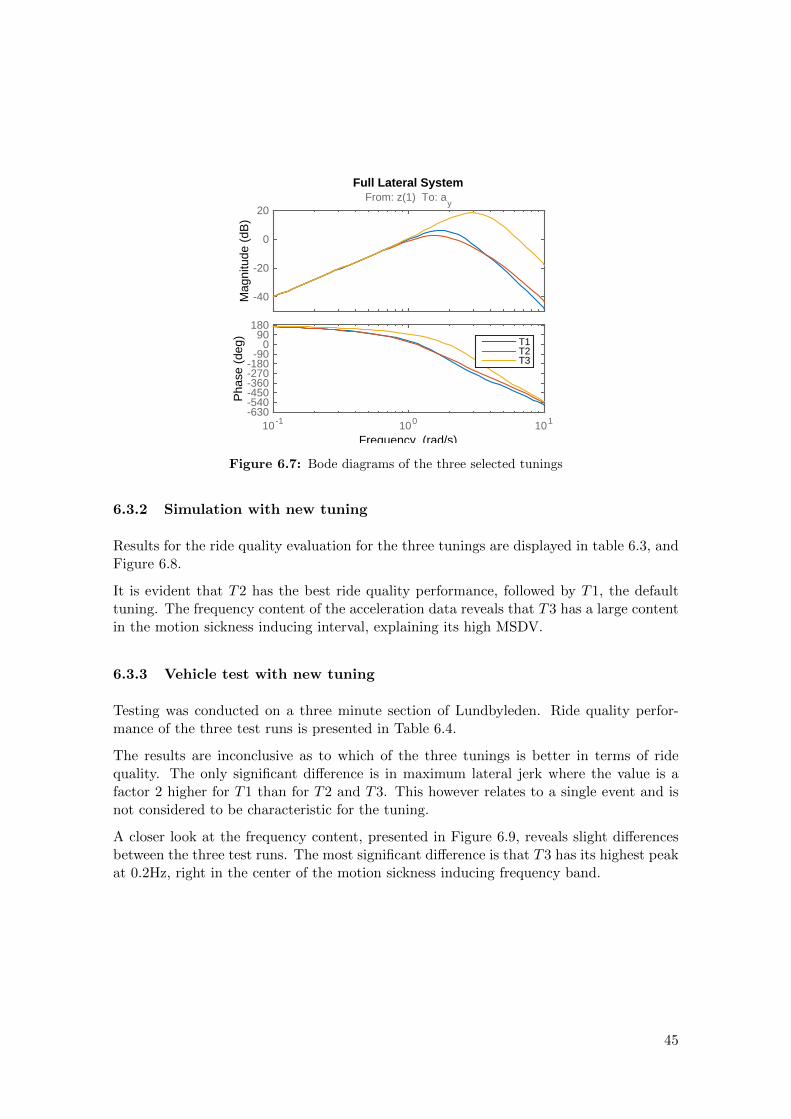
Mag

nitu

de (

dB)

-40

-20

0

20From: z(1) To: a

y

10 -1 100 101

Pha

se (

deg)

-630-540-450-360-270-180

-900

90180

T1T2T3

Full Lateral System

Frequency (rad/s)

Figure 6.7: Bode diagrams of the three selected tunings

6.3.2 Simulation with new tuning

Results for the ride quality evaluation for the three tunings are displayed in table 6.3, andFigure 6.8.

It is evident that T2 has the best ride quality performance, followed by T1, the defaulttuning. The frequency content of the acceleration data reveals that T3 has a large contentin the motion sickness inducing interval, explaining its high MSDV.

6.3.3 Vehicle test with new tuning

Testing was conducted on a three minute section of Lundbyleden. Ride quality perfor-mance of the three test runs is presented in Table 6.4.

The results are inconclusive as to which of the three tunings is better in terms of ridequality. The only significant difference is in maximum lateral jerk where the value is afactor 2 higher for T1 than for T2 and T3. This however relates to a single event and isnot considered to be characteristic for the tuning.

A closer look at the frequency content, presented in Figure 6.9, reveals slight differencesbetween the three test runs. The most significant difference is that T3 has its highest peakat 0.2Hz, right in the center of the motion sickness inducing frequency band.

45

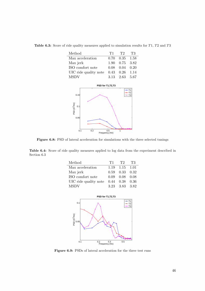
Table 6.3: Score of ride quality measures applied to simulation results for T1, T2 and T3

Method T1 T2 T3

Max acceleration 0.70 0.35 1.58Max jerk 1.90 0.75 3.82ISO comfort note 0.08 0.04 0.20UIC ride quality note 0.43 0.26 1.14MSDV 3.13 2.63 5.67

0.1 0.2 0.5 1

0.05

0.1

0.15

Frequency (Hz)

PS

D (

G2 /H

z)

PSD for T1,T2,T3

T1T2T3

Figure 6.8: PSD of lateral acceleration for simulations with the three selected tunings

Table 6.4: Score of ride quality measures applied to log data from the experiment described inSection 6.3

Method T1 T2 T3

Max acceleration 1.19 1.15 1.01Max jerk 0.59 0.33 0.32ISO comfort note 0.09 0.08 0.08UIC ride quality note 0.44 0.38 0.36MSDV 3.23 3.83 3.82

0.1 0.2 0.3 0.5

0.05

0.1

Frequency (Hz)

PS

D (

G2 /H

z)

PSD for T1,T2,T3

T1T2T3

Figure 6.9: PSDs of lateral acceleration for the three test runs

46

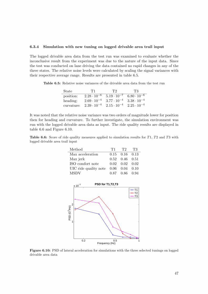
6.3.4 Simulation with new tuning on logged drivable area trail input

The logged drivable area data from the test run was examined to evaluate whether theinconclusive result from the experiment was due to the nature of the input data. Sincethe test was conducted on lane driving the data contained no rapid changes in any of thethree states. The relative noise levels were calculated by scaling the signal variances withtheir respective average range. Results are presented in table 6.5.

Table 6.5: Relative noise variances of the drivable area data from the test run

State T1 T2 T3

position: 2.28 · 10−6 5.19 · 10−7 6.80 · 10−6

heading: 2.69 · 10−4 3.77 · 10−4 3.38 · 10−4

curvature: 2.39 · 10−4 2.15 · 10−4 2.25 · 10−4

It was noted that the relative noise variance was two orders of magnitude lower for positionthen for heading and curvature. To further investigate, the simulation environment wasrun with the logged drivable area data as input. The ride quality results are displayed intable 6.6 and Figure 6.10.

Table 6.6: Score of ride quality measures applied to simulation results for T1, T2 and T3 withlogged drivable area trail input

Method T1 T2 T3

Max acceleration 0.15 0.16 0.13Max jerk 0.52 0.46 0.51ISO comfort note 0.02 0.02 0.02UIC ride quality note 0.06 0.04 0.10MSDV 0.87 0.86 0.94

0.2 0.5 1

1

2

x 10−3

Frequency (Hz)

PS

D (

G2 /H

z)

PSD for T1,T2,T3

T1T2T3

Figure 6.10: PSD of lateral acceleration for simulations with the three selected tunings on loggeddrivable area data

47

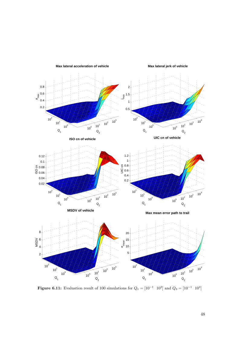
100 10

1 102 10

3

100

101

102

0.2

0.4

0.6

0.8

Q2

Max lateral acceleration of vehicle

Q1

a max

100 10

1 102 10

3

100

101

102

0.5

1

1.5

2

Q2

Max lateral jerk of vehicle

Q1

j max

100 10

1 102 10

3

100

101

102

0.02

0.04

0.06

0.08

0.1

0.12

Q2

ISO cn of vehicle

Q1

ISO

cn

100 10

1 102 10

3

100

101

102

0.2

0.4

0.6

0.8

1

1.2

Q2

UIC cn of vehicle

Q1

UIC

cn

100 10

1 102 10

3

100

101

102

2

4

6

8

Q2

MSDV of vehicle

Q1

MS

DV

100 10

1 102 10

3

100

101

102

5

10

15

20

Q2

Max mean error path to trail

Q1

e mea

n

Figure 6.11: Evaluation result of 100 simulations for Q1 = [10−1 103] and Q3 = [10−1 104]

48

Similar to the test results, these simulation result show little difference in ride qualityperformance between the three tunings. Although it was noted that the magnitude of theride quality measures and the PSD are significantly lower than for the experiment.

To evaluate whether the tuning process would yield a different ride quality optimal tuningfor the logged drivable area trail input the batch simulation script was run with the loggedinput data. Results are presented in Figure 6.11.

The decrease in ride quality at high values of Q1 is not as evident here but the same areas asin Figure 6.5 has the best ride quality. The resulting best tuning was [Q1 Q2 Q3] = [2 50 0]which is very close to the default tuning.

49

7Concluding remarks

This chapter summarizes the key finding of this thesis and discusses the implications of theresults. Some suggestions are also made for further experiments and development.

7.1 Conclusions

A strategy has been developed for tuning of a lateral path planning algorithm for anautonomous car that considers ride quality performance. The aim was to construct amethod for finding an optimal set of tuning parameters by considering a trade off betweenresponsiveness and ride quality. These quantities could be evaluated through a graphicaltool which was the result of development within three areas of functionality. A simulationenvironment, generating time domain responses for selected road scenarios, a frequencydomain analysis displaying the characteristics of a mathematical approximation of the pathplanner and methods for evaluating ride quality found through a literature study.

The collection of results from this thesis indicate that the tool fulfils its purpose to someextent, but there are areas in which more work is needed.

Several methods for determining ride quality were found and evaluated and were all con-sidered useful in the tuning process. The resulting ride quality evaluation functionality isvery flexible and easy to use since it only takes input of lateral acceleration. Thus, it canbe applied to simulation results from just about any vehicle simulation environment aswell as new or historic log data, since most test vehicles log lateral acceleration. Compar-ing different tunings to each other can be done through inspection of their correspondingride quality scores. However, the reference values to determine how well an individual setperforms need further evaluations through larger amounts of test data.

The frequency domain analysis shows the gain and phase responses for approximations ofthe path planner as well as the full lateral system. It displays for what tunings and fre-

50

quencies there is an amplification in lateral acceleration and for what range the controllerbecomes sensitive and should thus be avoided. The frequency analysis functionality wasuseful in understanding what tunings to avoid to have sufficiently low gain in the frequencyintervals related to discomfort and motion sickness.

The simulation environment was successful in the sense that it enabled analysis of thepath generation at arbitrary trail input. The simulation visualization functionality in thetool was useful in gaining understanding of the behaviour of the algorithm for differenttunings as well as analysis of the state initiation. However, the difference in magnitudeof ride quality parameters for the experiment and the simulation on logged drivable areatrail data points toward the conclusion that factors in the car control system that are notmodelled in the simulation environment dominate car behaviour. Delays in sensors andsensor fusion problems are candidates of such factors but analysis of these systems areoutside the scope of this project.

The process of gaining understanding of the tuning parameters evolved into a tuningstrategy based on batch simulations and ride quality evaluation. The concept is to compareride quality scores of different tunings for the same road scenario using 2D graphics forsingle tuning parameters, or 3D graphics for two tuning parameters at the time. Initially, astep scenario was chosen, for which the tool generated a clear result of which tuning is ridequality optimal under a constraint of minimum responsiveness. Subsequently, the processwas reiterated for logged drivable area data, yielding a different optimal tuning, with a lessclear distinction in performance between different tunings. The main explanation is mostlikely the limited amount of data and that it was collected only during lane following. Fromthis it was concluded that the method needs a simulation scenario that is representative ofthe situation where one wants to optimize ride quality. A natural choice for input data islogged data from a test run. However, the drivable area trail is logged in the car coordinatesystem and is therefore a superposition of its placement in the world coordinate systemand the motion of the vehicle. Ideally, drivable area trail input data for simulations shouldbe collected when driving in manual mode so the data is not tainted by oscillating motionsin the logging vehicle.

No conclusive improvements in ride quality could be achieved through retuning the pathplanning algorithm, using the new methods. However, to fully evaluate whether ride qual-ity based tuning is a good strategy more tests in vehicle need to be performed, includinga broader variety of motion. The short test runs of three minutes may have been tooshort and uneventful to generate a measurable difference in car behaviour for the threetunings. A longer test run would have given more data, a higher resolution of the ac-celeration PSD for low frequencies and exposed the control system to a more diverse setof drivable area input data, but was not possible at the testing occasion due to externalreasons. For further evaluation of the ride quality based tuning process, longer test runsare recommended.

A conclusion that was made from comparing simulated and measured data is that theapproximations of the simulation environment makes it unable to capture all the relevantdynamics of the vehicle. This is probably one of the reasons for the reduced ability to findbetter tuning sets. If used with a more accurate simulation environment and representativesimulation scenarios we believe that there are good prospects for the tuning strategy

51

developed here.

In a broader perspective, the concept of using quantitative ride quality measures appearsto be a promising way forward in development and tuning of motion controllers in au-tonomous vehicles.

7.2 Ideas for further development

A way of improving the tuning strategy is to add information. When the process wascarried out to find an optimal tuning 3D plots were very helpful to get a clear overview ofthe performance of different combinations of tunings on ride quality and responsiveness.These 3D plots could be integrated in the tool to enable a faster process, since it showsseveral tunings at a time. A second addition would be to vary all three tuning parameterssimultaneously, in this project we were restricted to keeping one variable fixed due to thecomputational burden.

The next step for improving ride quality for autonomous driving is to use the knowledgeof which frequency bands to avoid in the design of the controller itself. This may be a wayaround the trade off between ride quality and responsiveness. An effective possibility forthis is to use a Frequency Shaped Linear Quadratic Regulator, FSLQ, instead of the LQT.An FSLQ has frequency-dependent weighting matrices in the cost function, allowing formore design freedom. The implication is a possibility to reduce gain in the interval 0.1-0.5Hz, causing motion sickness. It would have to be determined if that had any negativeimpact on responsiveness, if not the FSLQ may be an opportunity for good ride qualityin autonomous cars, [18]

We believe that there may be potential benefit in using the ride quality evaluation func-tionality in combination with the SPAS simulation environment used for validation andverification purposes. The SPAS environment contains a detailed vehicle model and all ofthe AD functionality as opposed to the simplified lateral environment used in this work.The problems here with the simulation model failing to reproduce similar ride qualityscore to that of the test vehicle when run on the same input data may be less evident withSPAS. Reproducing the batch simulation tuning process with SPAS run on a representativescenario could provide interesting results.

One issue to highlight is that the development of the path planner and lateral controllerused in the cars are under constant development. For an accurate analysis the tool has tobe updated accordingly. At the time of this writing the lateral control group are workingon a controller that follows the path planner reference more carefully. This will have effecton the simulation environment used in the tool, which now contains non-linearities thatwill disregard aggressive path data. A second effect is that it puts higher demands on theperformance of the path planner, suggesting a greater need of a tuning tool.

52

8References

[1] International Organization for Standardization. ISO 2631-1:. International standard.ISO, 1997.

[2] International Organization for Standardization. ISO 2631-4:. International standard.ISO, 2001.

[3] J. Forstberg. Influence from horizontal and/or roll motion on nausea and motionsickness : Experiments in a moving vehicle simulator. Technical report, SwedishNational Road and Transport Research Institute, 2000.

[4] J. Forstberg. Ride comfort and motion sickness in tilting trains. PhD thesis, RoyalInstitute of Technology (KTH), 2000.

[5] Golding JF et. al. A motion sickness maximum around the 0.2 hz frequency rangeof horizontal translational oscillation. Aviation, Space, and Environmental Medicine,72:pp. 188–92, March 2001.

[6] MJ. Griffin and RA. Hayward. Effects of horizontal whole-body vibration on reading.Applied Ergonomics, pages pp. 165–169, 1994.

[7] BE. Donohew and MJ. Griffin. Motion sickness: effect of the frequency of lateraloscillation. Aviation, Space, and Environmental Medicine, 75:pp. 649–656, August2004.

[8] A. Kilinc and A. Baybura. Determination of minimum horizontal curve radius usedin the design of transportation structures, depending on the limit value of comfortcriterion lateral jerk. In Proceedings of Knowing to manage the territory, protect theenvironment, evaluate the cultural heritage, May 2012.

53

[9] K. Kottenhoff. Samband mellan korstil och akkomfort–forbattringspotentialen inomkollektivtrafiken. Technical report, FoKoll, Forskningsgruppen for KollektivtrafikTrafik & Logistik, KTH, 2011.

[10] G. Lauriks et al. Uic comfort tests : Investigation of ride comfort and comfortdisturbance on transition and circular curves. Technical report, Swedish NationalRoad and Transport Research Institute, 2003.

[11] J. Sundstrom and S. Khan. Influence of stationary lateral vibrations on train passen-gers’ difficulty to read and write. Applied Ergonomics, page pp. 710–718, 2008.

[12] M. Turner and MJ. Griffin. Motion sickness in public road transport: the effect ofdriver, route and vehicle. Ergonomics, 42:pp. 1646–1664, 1999.

[13] N. Karlsson and H. Tjarnbro. Motion sickness in cars. diploma thesis, ChalmersUniversity of Technology, 2012.

[14] D.S. Naidu. Optimal Control Systems. CRC Press, 2003.

[15] R. Rajamani. Vehicle Dynamics and Control. Butterworth-Heinemann, 2006.

[16] P. Stoica and R. Moses. Spectral analysis of signals. PHI Learning Privat Ltd, 2005.

[17] S. Boyd. Infinite horizon linear quadratic regulator. http://stanford.edu/class/

ee363/lectures/dlqr-ss.pdf, 2008.

[18] X. Chen. Lq with frequency shaped cost function. http://www.me.berkeley.edu/

ME233/sp14/_static/UCB_ME233_10_frequency_shaped_lq.pdf, 2014.

[19] O. Egeland and E. Lunde. Trajectory generation for manipulators using linearquadratic optimal tracking. In Robotics and Automation, 1988. Proceedings., 1988IEEE International Conference on, pages 376–381 vol.1, Apr 1988.

[20] Ali M. Decision Making and Control for Automotive Safety. PhD thesis, ChalmersUniversity of Technology, 2012.

[21] National Highway Traffic Safety Administration. Policy on automated vehicle devel-opment. http://www.nhtsa.gov, 2013.

[22] Volvo Car Group. Autonom korning enligt volvo car group. http://www.

mynewsdesk.com/se/, 2013.

[23] Unknown author. ’phantom auto’ will tour city. The Milwaukee Sentinel, page pp. 4,1926.

[24] M. Weber. Where to? a history of autonomous vehicles. http://www.

computerhistory.org, 2014.

54

Appendices

55

APreparation of data

In order to use some of the ride quality evaluation methods in this thesis data needed tobe processed. The methods are presented below.

A.1 Acceleration and Jerk

The acceleration data needed to be pre processed prior to applying the comfort evaluationmethods. By utilizing the Rauch-Tung-Striebel formulas both filtered acceleration andjerk could be computed in a few steps. This was achieved by using the model[

y(k + 1)...y (k + 1)

]=

[1 dt0 1

] [y(k)...y (k)

]z(k) =

[1 0

] [ y(k)...y (k)

] (A.1)

where y(k) is the acceleration data,...y (k) is jerk, z(k) is the output signal and dt is the time

step between each sample. This method of processing data proved to be more successfulthan using for example a low pass filter since the relation between acceleration and jerkcould be utilized.

A.1.1 The Rauch-Tung-Striebel (RTS) formulas

The Rauch-Tung-Striebel formulas, also known as Kalman smoother, can be used for off-line smoothing of data belonging to a known model. It is a fixed-interval smoother in twosteps; step 1 is forward filtering using the Kalman filter equations, step 2 is backwardssmoothing.

56

Step 1 forward: Kalman filteringGiven the model

x(k) = Ax(k) +Bu(k)

y(k) = Cx(k) +Du(k)(A.2)

and measurements y(1)...y(N), the filtered states x(k|k) can be computed through theequations

x(k|k − 1) = Ax(k − 1|k − 1) +B(k)u(k)

P (k|k − 1) = AP (k − 1|k − 1)AT +Q

K(k) = P (k|k − 1)CT [CP (k|k − 1)CT +R]−1

x(k|k) = x(k|k − 1) +K(y(k)− Cx(k|k − 1))

P (k|k) = (I −KC)P (k|k − 1)

(A.3)

where K(k) is the Kalman gain, x(k|k−1) is the predicted state estimate vector, P (k|k−1)is the predicted estimate covariance matrix and P (k|k) is the filtered estimate covariance.R is the variance of the measurement noise and Q is the variance of the process noise,however these parameters can also be regarded as design parameters and can therefore bealtered in order to achieve satisfying results.

Step 2 backwards: RTS smoothingThrough the Kalman predictions and filtered estimates x(k|k), x(k|k − 1), P (k|k),P (k|k − 1) the smoothed state vector is computed as

x(k|N) = x(k|k) + C(k)(x(k + 1|N)− x(k + 1|k))

P (k|N) = P (k|k) + C(k)(P (k + 1|N)− x(k + 1|k))CT (k)

C(k) = P (k|k)ATP (k + 1|k)−1

(A.4)

where x(k|N) is the smoothed state vector and P (k|N) is the smoothed covariance vec-tor.

A.2 ISO and UIC filters

This section contains detailed information on the transfer functions used to calculatefrequency weighted acceleration data for ride quality evaluation.

A.2.1 ISO 2631-1 filters

The transfer functions of the for ISO 2631-1 filters, Wc, Wd and Wf are constructed usingequation A.5.

HW (s) = Hh(s) ·Hl(s) ·Ht(s) ·Hs(s) (A.5)

57

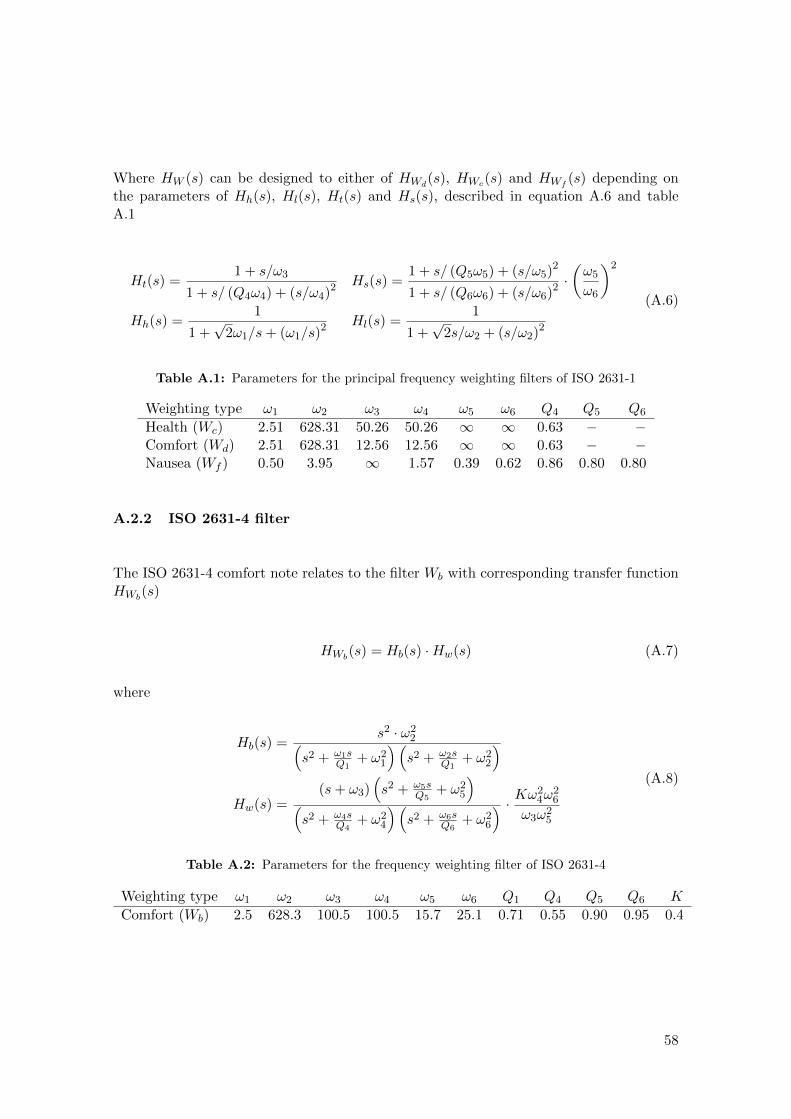
Where HW (s) can be designed to either of HWd(s), HWc(s) and HWf

(s) depending onthe parameters of Hh(s), Hl(s), Ht(s) and Hs(s), described in equation A.6 and tableA.1

Ht(s) =1 + s/ω3

1 + s/ (Q4ω4) + (s/ω4)2 Hs(s) =

1 + s/ (Q5ω5) + (s/ω5)2

1 + s/ (Q6ω6) + (s/ω6)2 ·(ω5

ω6

)2

Hh(s) =1

1 +√

2ω1/s+ (ω1/s)2 Hl(s) =

1

1 +√

2s/ω2 + (s/ω2)2

(A.6)

Table A.1: Parameters for the principal frequency weighting filters of ISO 2631-1

Weighting type ω1 ω2 ω3 ω4 ω5 ω6 Q4 Q5 Q6

Health (Wc) 2.51 628.31 50.26 50.26 ∞ ∞ 0.63 − −Comfort (Wd) 2.51 628.31 12.56 12.56 ∞ ∞ 0.63 − −Nausea (Wf ) 0.50 3.95 ∞ 1.57 0.39 0.62 0.86 0.80 0.80

A.2.2 ISO 2631-4 filter

The ISO 2631-4 comfort note relates to the filter Wb with corresponding transfer functionHWb

(s)

HWb(s) = Hb(s) ·Hw(s) (A.7)

where

Hb(s) =s2 · ω2

2(s2 + ω1s

Q1+ ω2

1

)(s2 + ω2s

Q1+ ω2

2

)Hw(s) =

(s+ ω3)(s2 + ω5s

Q5+ ω2

5

)(s2 + ω4s

Q4+ ω2

4

)(s2 + ω6s

Q6+ ω2

6

) · Kω24ω

26

ω3ω25

(A.8)

Table A.2: Parameters for the frequency weighting filter of ISO 2631-4

Weighting type ω1 ω2 ω3 ω4 ω5 ω6 Q1 Q4 Q5 Q6 K

Comfort (Wb) 2.5 628.3 100.5 100.5 15.7 25.1 0.71 0.55 0.90 0.95 0.4

58

A.3 UIC ride quality note

The data used in the UIC comfort note,

UIC rq note = 0.094NV A + 0.6y50 + 0.37...y 50

was prepared according to methods described in the report. NV A is computed accordingto the CEN-standard, see section 2.2.4. To get the 50th-percentiles some preparation isrequired. Low-pass filtered acceleration data is reduced to samples of length 0.1 s by takingthe average value on each 0.1 s interval. This data is further divided into sections of length5 min. Each 5 min interval is then reduced by only taking the maximum acceleration oneach 5 s interval. At last the 50th percentile is taken on each 5 min interval.

59

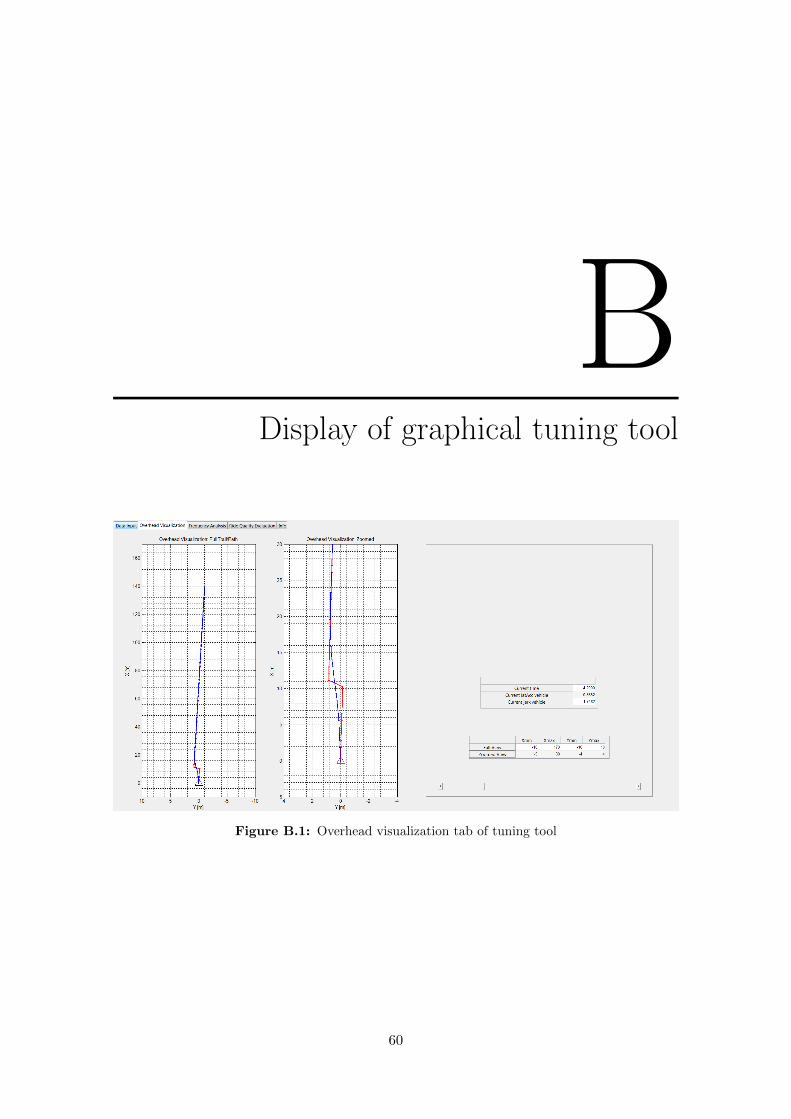
BDisplay of graphical tuning tool

Figure B.1: Overhead visualization tab of tuning tool

60

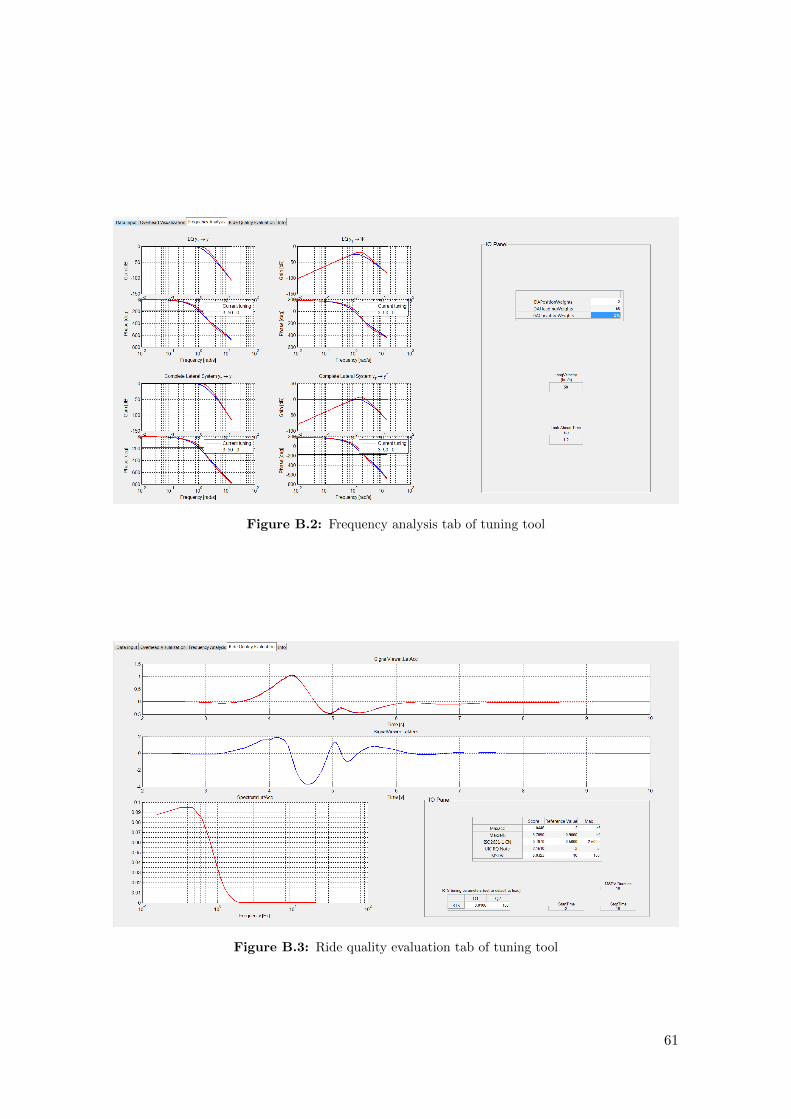
Figure B.2: Frequency analysis tab of tuning tool

Figure B.3: Ride quality evaluation tab of tuning tool

61