Embed Size (px)
Citation preview

Utah State University Utah State University
DigitalCommons@USU DigitalCommons@USU
All Graduate Theses and Dissertations Graduate Studies
8-2019
Tuning Hyperparameters in Supervised Learning Models and Tuning Hyperparameters in Supervised Learning Models and
Applications of Statistical Learning in Genome-Wide Association Applications of Statistical Learning in Genome-Wide Association
Studies with Emphasis on Heritability Studies with Emphasis on Heritability
Jill F. Lundell Utah State University
Follow this and additional works at: https://digitalcommons.usu.edu/etd
Part of the Statistics and Probability Commons
Recommended Citation Recommended Citation Lundell, Jill F., "Tuning Hyperparameters in Supervised Learning Models and Applications of Statistical Learning in Genome-Wide Association Studies with Emphasis on Heritability" (2019). All Graduate Theses and Dissertations. 7594. https://digitalcommons.usu.edu/etd/7594
This Dissertation is brought to you for free and open access by the Graduate Studies at DigitalCommons@USU. It has been accepted for inclusion in All Graduate Theses and Dissertations by an authorized administrator of DigitalCommons@USU. For more information, please contact [email protected].

TUNING HYPERPARAMETERS IN SUPERVISED LEARNING MODELS AND
APPLICATIONS OF STATISTICAL LEARNING IN GENOME-WIDE ASSOCIATION
STUDIES WITH EMPHASIS ON HERITABILITY
by
Jill F. Lundell
A dissertation submitted in partial fulfillmentof the requirements for the degree
of
DOCTOR OF PHILOSOPHY
in
Mathematical Sciences
(Statistics)
Approved:
D. Richard Cutler, Ph.D. Chris D. Corcoran, Sc.D.Major Professor Committee Member
Adele Cutler, Ph.D. Zachariah Gompert, Ph.D.Committee Member Committee Member
Jurgen Symanzik, Ph.D. Richard S. Inouye, Ph.D.Committee Member Vice Provost for Graduate Studies
UTAH STATE UNIVERSITYLogan, Utah
2019

ii
Copyright c© Jill F. Lundell 2019
All Rights Reserved

iii
ABSTRACT
Tuning Hyperparameters in Supervised Learning Models and Applications of Statistical
Learning in Genome-Wide Association Studies with Emphasis on Heritability
by
Jill F. Lundell, Doctor of Philosophy
Utah State University, 2019
Major Professor: D. Richard Cutler, Ph.D.Department: Mathematics and Statistics
Statistical learning models have been growing in popularity in recent years. Many of
these methods have parameters that must be tuned for models to perform well. Research
has been extensive in neural networks, but not for other learning methods. We look at the
behavior of tuning parameters for support vector machines, gradient boosting machines,
and adaboost in both a classification and regression setting. We found ranges of tuning
parameters where good solutions can be found across many different datasets. We then
explored different optimization algorithms to search for a good set of parameters across
that space. This information was used to create an R package, EZtune, that automatically
tunes learning models.
In the second part of this dissertation, we explore of the use of traditional and statis-
tical learning methods in genome-wide association studies. We simulated data using high
heritability and low heritability. Distance correlation and linear and logistic regression were
evaluated as first-phase filters to remove the majority of the noise from the data. Elastic
net was then investigated as a tool for secondary filtering. Random forests and classification
and regression trees were used for final single nucleotide polymorphism (SNP) selection. We

iv
assessed the affect of heritability through all of these stages as the ability of each method
to find target SNPs.
(119 pages)

v
PUBLIC ABSTRACT
Tuning Hyperparameters in Supervised Learning Models and Applications of Statistical
Learning in Genome-Wide Association Studies with Emphasis on Heritability
Jill F. Lundell
Machine learning is a buzz word that has inundated popular culture in the last few
years. This is a term for a computer method that can automatically learn and improve from
data instead of being explicitly programmed at every step. Investigations regarding the best
way to create and use these methods are prevalent in research. Machine learning models
can be difficult to create because models need to be tuned. This dissertation explores
the characteristics of tuning three popular machine learning models and finds a way to
automatically select a set of tuning parameters. This information was used to create an R
software package called EZtune that can be used to automatically tune three widely used
machine learning algorithms: support vector machines, gradient boosting machines, and
adaboost.
The second portion of this dissertation investigates the implementation of machine
learning methods in finding locations along a genome that are associated with a trait. The
performance of methods that have been commonly used for these types of studies, and some
that have not been commonly used, are assessed using simulated data. The affect of the
strength of the relationship between the genetic code and the trait is of particular interest.
It was found that the strength of this relationship was the most important characteristic in
the efficacy of each method.

vi
ACKNOWLEDGMENTS
I would like to thank my advisor, Richard Cutler, for his expertise, advice, and patience
while I tried to decide on a topic and for continuing to provide great insights during the
process. I would also like to thank Adele Cutler for being so generous with her knowledge
of optimization and statistical learning, Jurgen Symanzik for mentoring me on graphics and
precision, Zach Gompert for sharing his expertise in genetics with me, Chris Corcoran for
providing me with invaluable opportunities in my graduate program, and Guifang Fu for
giving me the opportunity to dive into genetics in the first place.
I would also like to thank my family for their support and patience with this crazy
journey.
Jill F. Lundell

vii
CONTENTS
Page
ABSTRACT . . . . . . . . . . . . . . . . . . . . . . . . . . . . . . . . . . . . . . . . . . . . . . . . . . . . . . iii
PUBLIC ABSTRACT . . . . . . . . . . . . . . . . . . . . . . . . . . . . . . . . . . . . . . . . . . . . . . . v
ACKNOWLEDGMENTS . . . . . . . . . . . . . . . . . . . . . . . . . . . . . . . . . . . . . . . . . . . . vi
LIST OF TABLES . . . . . . . . . . . . . . . . . . . . . . . . . . . . . . . . . . . . . . . . . . . . . . . . . ix
LIST OF FIGURES . . . . . . . . . . . . . . . . . . . . . . . . . . . . . . . . . . . . . . . . . . . . . . . . xi
ACRONYMS . . . . . . . . . . . . . . . . . . . . . . . . . . . . . . . . . . . . . . . . . . . . . . . . . . . . . xiii
1 INTRODUCTION . . . . . . . . . . . . . . . . . . . . . . . . . . . . . . . . . . . . . . . . . . . . . . . 11.1 Introduction . . . . . . . . . . . . . . . . . . . . . . . . . . . . . . . . . . . . 11.2 Overview of Statistical Learning Methods . . . . . . . . . . . . . . . . . . . 21.3 Statistical Model Parameter Tuning Literature Review and Background . . 7
1.3.1 Genome-Wide Association Study Literature Review and Background 9
2 TUNING SUPERVISED LEARNING METHODS . . . . . . . . . . . . . . . . . . . . . . . . 122.1 Introduction . . . . . . . . . . . . . . . . . . . . . . . . . . . . . . . . . . . . 122.2 Optimization Algorithms . . . . . . . . . . . . . . . . . . . . . . . . . . . . 122.3 Methods . . . . . . . . . . . . . . . . . . . . . . . . . . . . . . . . . . . . . . 13
2.3.1 Grid Search . . . . . . . . . . . . . . . . . . . . . . . . . . . . . . . . 132.3.2 Optimization Algorithms . . . . . . . . . . . . . . . . . . . . . . . . 15
2.4 Results . . . . . . . . . . . . . . . . . . . . . . . . . . . . . . . . . . . . . . . 182.4.1 Results of Grid Search . . . . . . . . . . . . . . . . . . . . . . . . . . 202.4.2 Results of Optimization Algorithms . . . . . . . . . . . . . . . . . . 24
2.5 Conclusions . . . . . . . . . . . . . . . . . . . . . . . . . . . . . . . . . . . . 25
3 EZTUNE: AN R PACKAGE FOR AUTOMATIC TUNING OF SUPPORT VEC-TOR MACHINES, GRADIENT BOOSTING MACHINES, AND ADABOOST . . . . . 31
3.1 Introduction . . . . . . . . . . . . . . . . . . . . . . . . . . . . . . . . . . . . 313.2 Package Components and How to Use Them . . . . . . . . . . . . . . . . . . 33
3.2.1 Datasets . . . . . . . . . . . . . . . . . . . . . . . . . . . . . . . . . . 333.2.2 Automatic Tuning with eztune . . . . . . . . . . . . . . . . . . . . . 353.2.3 Model Performance Verification with eztune cv . . . . . . . . . . . 39
3.3 Performance and Benchmarking . . . . . . . . . . . . . . . . . . . . . . . . . 403.4 Conclusions . . . . . . . . . . . . . . . . . . . . . . . . . . . . . . . . . . . . 42

viii
4 THREE-PHASE FILTERING METHOD FOR GENOME-WIDE ASSOCIATIONSTUDIES . . . . . . . . . . . . . . . . . . . . . . . . . . . . . . . . . . . . . . . . . . . . . . . . . . . . . . . . 54
4.1 Introduction . . . . . . . . . . . . . . . . . . . . . . . . . . . . . . . . . . . . 544.2 Method . . . . . . . . . . . . . . . . . . . . . . . . . . . . . . . . . . . . . . 55
4.2.1 Data Simulation . . . . . . . . . . . . . . . . . . . . . . . . . . . . . 564.2.2 Initial Filtering . . . . . . . . . . . . . . . . . . . . . . . . . . . . . . 574.2.3 LASSO and Elastic Net for Further Refinement . . . . . . . . . . . . 594.2.4 Random Forests and Classification and Regression Trees for Final
SNP Selection . . . . . . . . . . . . . . . . . . . . . . . . . . . . . . . 594.2.5 Final Assessment of Results . . . . . . . . . . . . . . . . . . . . . . . 59
4.3 Results . . . . . . . . . . . . . . . . . . . . . . . . . . . . . . . . . . . . . . . 624.3.1 Heritability . . . . . . . . . . . . . . . . . . . . . . . . . . . . . . . . 624.3.2 Initial Filter . . . . . . . . . . . . . . . . . . . . . . . . . . . . . . . . 624.3.3 Elastic Net . . . . . . . . . . . . . . . . . . . . . . . . . . . . . . . . 634.3.4 Random Forests and CART . . . . . . . . . . . . . . . . . . . . . . . 744.3.5 Datasets . . . . . . . . . . . . . . . . . . . . . . . . . . . . . . . . . . 74
4.4 Conclusions . . . . . . . . . . . . . . . . . . . . . . . . . . . . . . . . . . . . 74
5 FUTURE WORK AND CONCLUSIONS . . . . . . . . . . . . . . . . . . . . . . . . . . . . . . 76
APPENDICES . . . . . . . . . . . . . . . . . . . . . . . . . . . . . . . . . . . . . . . . . . . . . . . . . . . . 78A EZtune Vignette . . . . . . . . . . . . . . . . . . . . . . . . . . . . . . . . . 79
A.1 Introduction to EZtune . . . . . . . . . . . . . . . . . . . . . . . . . 79A.2 Functions: eztune and eztune cv . . . . . . . . . . . . . . . . . . . . 79A.3 Datasets . . . . . . . . . . . . . . . . . . . . . . . . . . . . . . . . . . 84A.4 Examples . . . . . . . . . . . . . . . . . . . . . . . . . . . . . . . . . 86A.5 Performance and speed guidelines . . . . . . . . . . . . . . . . . . . 89
B Guide to Dissertation Code . . . . . . . . . . . . . . . . . . . . . . . . . . . 91B.1 Tuning Research . . . . . . . . . . . . . . . . . . . . . . . . . . . . . 91B.2 EZtune . . . . . . . . . . . . . . . . . . . . . . . . . . . . . . . . . . 93B.3 GWAS Work . . . . . . . . . . . . . . . . . . . . . . . . . . . . . . . 94
REFERENCES . . . . . . . . . . . . . . . . . . . . . . . . . . . . . . . . . . . . . . . . . . . . . . . . . . . 96
CURRICULUM VITAE . . . . . . . . . . . . . . . . . . . . . . . . . . . . . . . . . . . . . . . . . . . . . 102

ix
LIST OF TABLES
Table Page
2.1 List of datasets used to explore tuning parameters. . . . . . . . . . . . . . . 14
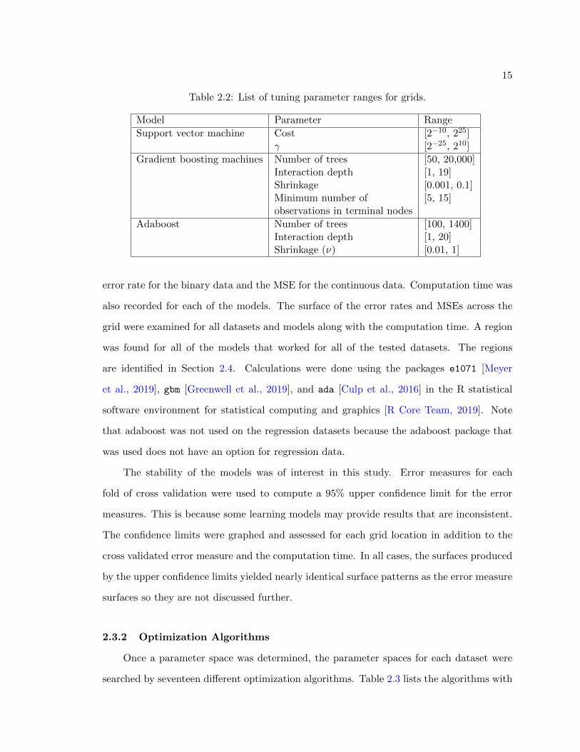
2.2 List of tuning parameter ranges for grids. . . . . . . . . . . . . . . . . . . . 15
2.3 List of optimization algorithms used to search tuning parameter spaces witha brief description of each method. . . . . . . . . . . . . . . . . . . . . . . . 16
2.4 List of optimization algorithms along with the packages and functions in Rthat will be used to implement them. . . . . . . . . . . . . . . . . . . . . . . 19
2.5 List of recommended tuning parameter spaces for binary classification modelsbased on grid search. . . . . . . . . . . . . . . . . . . . . . . . . . . . . . . . 22
2.6 List of recommended tuning parameter spaces for regression models basedon grid search. . . . . . . . . . . . . . . . . . . . . . . . . . . . . . . . . . . 23
2.7 Performance summary of optimization algorithms. . . . . . . . . . . . . . . 25
3.1 Average mean squared errors from cross validation model verification andcomputation times in seconds for support vector regression with EZtune.The best mean squared errors from the grid search are included in the tablefor reference. Table entries are (cross validated MSE, computation time inseconds). . . . . . . . . . . . . . . . . . . . . . . . . . . . . . . . . . . . . . . 43
3.2 Average mean squared errors from cross validation model verification andcomputation times in seconds for gradient boosting regression with EZtune.The best mean squared errors from the grid search are included in the tablefor reference. Table entries are (cross validated MSE, computation time inseconds). . . . . . . . . . . . . . . . . . . . . . . . . . . . . . . . . . . . . . . 45
3.3 Average classification errors from cross validation model verification and com-putation times in seconds for support vector classification with EZtune. Thebest classification errors from the grid search are included in the table forreference. Table entries are (cross validated error rate, computation time inseconds). . . . . . . . . . . . . . . . . . . . . . . . . . . . . . . . . . . . . . . 47
3.4 Average classification errors from cross validation model verification and com-putation times in seconds for gradient boosting classification with EZtune.The best classification errors from the grid search are included in the tablefor reference. Table entries are (cross validated error rate, computation timein seconds). . . . . . . . . . . . . . . . . . . . . . . . . . . . . . . . . . . . . 49

x
3.5 Average classification errors from cross validation model verification and com-putation times in seconds for adaboost with EZtune. The best classificationerrors from the grid search are included in the table for reference. Tableentries are (cross validated error rate, computation time in seconds). . . . . 51
4.1 List of datasets used for data simulation. . . . . . . . . . . . . . . . . . . . . 56

xi
LIST OF FIGURES
Figure Page
2.1 Error surface plots for support vector machines on datasets with a binaryresponse. The orange dots on the bottom figure represent the best 20 modelsacross the grid. . . . . . . . . . . . . . . . . . . . . . . . . . . . . . . . . . . 21
2.2 Computation time surface plots for support vector machines on datasets witha binary response. The orange dots represent the 20 models with the shortestcomputation times across the grid. Time is in seconds. . . . . . . . . . . . . 22
2.3 Standardized optimization results for support vector machines for regression. 26
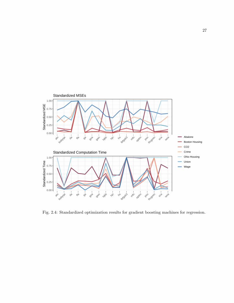
2.4 Standardized optimization results for gradient boosting machines for regression. 27
2.5 Standardized optimization results for support vector machines for binaryclassification. . . . . . . . . . . . . . . . . . . . . . . . . . . . . . . . . . . . 28
2.6 Standardized optimization results for gradient boosting machines for binaryclassification. . . . . . . . . . . . . . . . . . . . . . . . . . . . . . . . . . . . 29
2.7 Standardized optimization results for adaboost models for binary classification. 30
3.1 Standardized mean squared error results and computation times for supportvector regression. The best mean squared errors and computation times foreach dataset have a value of 0 and the worst have a value of 1. . . . . . . . 44
3.2 Standardized mean squared error results and computation times for gradientboosting regression. The best mean squared errors and computation timesfor each dataset have a value of 0 and the worst have a value of 1. . . . . . 46
3.3 Standardized classification error rates and computation times for supportvector classification. The best error rates and computation times for eachdataset have a value of 0 and the worst have a value of 1. . . . . . . . . . . 48
3.4 Standardized classification error rates and computation times for gradientboosting classification. The best error rates and computation times for eachdataset have a value of 0 and the worst have a value of 1. . . . . . . . . . . 50
3.5 Standardized classification error rates and computation times for adaboost.The best error rates and computation times for each dataset have a value of0 and the worst have a value of 1. . . . . . . . . . . . . . . . . . . . . . . . 52

xii
4.1 Example plot for assessing the performance of the GWAS method with themouse data. The radius of the green circles represents the importance asdetermined by random forests. The blue circles represent the SNPs thattrees found to be important and purple circles represent the SNPs with non-zero coefficients in the elastic net model. The radius of the blue and purplecircles does not represent anything. The red lines show the position of thefunctional SNPs. . . . . . . . . . . . . . . . . . . . . . . . . . . . . . . . . . 61
4.2 NMRI mouse data with heritability of 0.1 demonstrating inability of filter tofind truly associated SNPs. . . . . . . . . . . . . . . . . . . . . . . . . . . . 64
4.3 NMRI mouse data with heritability of 0.3 demonstrating inability of filter tofind truly associated SNPs. . . . . . . . . . . . . . . . . . . . . . . . . . . . 65
4.4 NMRI mouse data with heritability of 0.8 demonstrating improvement inmethod with stronger heritability. . . . . . . . . . . . . . . . . . . . . . . . . 66
4.5 T. cristinae data with heritability of 0.1 demonstrating inability of filter tofind truly associated SNPs. . . . . . . . . . . . . . . . . . . . . . . . . . . . 67
4.6 T. cristinae data with heritability of 0.3 demonstrating inability of filter tofind truly associated SNPs. . . . . . . . . . . . . . . . . . . . . . . . . . . . 68
4.7 T. cristinae data with heritability of 0.8 demonstrating improvement inmethod with stronger heritability. . . . . . . . . . . . . . . . . . . . . . . . . 69
4.8 R. pomonella data with heritability of 0.3 and with the linear regression filterusing the FDR p-values transformed using − log10 P . This plot demonstratesinability of filter to find truly associated SNPs with such low heritability andthe difference in the filter plot between FDR p-values and raw p-values. . . 70
4.9 R. pomonella data with heritability of 0.3 and with the linear regression filterwith the raw p-values transformed using − log10 P . This plot demonstratesinability of filter to find truly associated SNPs with such low heritabilityand the difference in the filter plot between distance correlation, the FDRp-values, and raw p-values. . . . . . . . . . . . . . . . . . . . . . . . . . . . 71
4.10 R. pomonella data with heritability of 0.3 and with the distance correlationfilter. This plot demonstrates inability of filter to find truly associated SNPswith such low heritability and the difference in the filter plot between distancecorrelation, the FDR p-values, and raw p-values. . . . . . . . . . . . . . . . 72
4.11 R. pomonella data with heritability of 0.8 demonstrating improvement inmethod with stronger heritability. . . . . . . . . . . . . . . . . . . . . . . . . 73

xiii
ACRONYMS
CART classification and regression trees
CVS Current Vegetation Survey
FDR false discovery rate
GBM gradient boosting machine
GWAS genome-wide association study
LASSO least absolute shrinkage and selection operator
LD linkage disequilibrium
MSE mean squared error
OOB out-of-bag
SNP single nucleotide polymorphism
SVM support vector machines
SVR support vector regression
WTCCC Wellcome Trust Case Control Consortium

CHAPTER 1
INTRODUCTION
1.1 Introduction
Machine learning is discipline consisting of algorithms than can learn from data without
explicit rule based programming. Statistical learning is machine learning within a statis-
tical framework. Statistical learning may or may not be probabilistic, have distributional
assumptions, be used for prediction or inference, but the primary distinction is that there
is greater concern with the balance between prediction accuracy and model interpretability
than machine learning in general.
Statistical learning models have gained in popularity in recent years because of their
ability to provide greater accuracy than statistical methods in many situations. Random
forests is a statistical learning method that performs well without parameter tuning, but
most learning methods have parameters that must be tuned for the models to perform
well [Breiman, 2001]. The No Free Lunch theorems state that there is no one type of
model that outperforms all other models in all situations [Schumacher et al., 2001]. Thus,
having several different types of models to address a problem is essential to finding a good
solution. Support vector machines (SVMs) [Cortes and Vapnik, 1995], gradient boosting
machines (GBMs) [Friedman, 2001], and adaboost [Freund and Schapire, 1997] are three
supervised learning models that perform well if tuned. Parameters can be difficult to tune
and recommendations for tuning methods are not well justified. Better understanding of
the properties of tuning parameters and how to tune them is needed. Software tools that
allow users to tune models without requiring the user to do substantial research are also
lacking. Further development of tuning software would provide many data analysts with a
wide range of more accessible tools for modeling.
When machine learning models were first developed it was hoped that they could

2
emulate the brain and provide better understanding of how the brain worked. This goal
was eventually abandoned, but in recent years learning methods have been used to try to
better understand the structure of data and of natural systems. One example of this is the
use of least absolute shrinkage and selection operator (LASSO) in finding locations across
genomes that contribute to a disease or physical trait [Wu et al., 2009]. This area of research
is still new and questions about how to tune and implement learning methods to address
such questions abound.
In Chapter 2, we explore tuning parameters for SVM, GBM, and adaboost to find the
parameter spaces that yield good predictive models. We then use different optimization
algorithms to search over the parameter spaces to find a set of tuning parameters that
produce a good model for each of the model types. This information is used to create an
R package called EZtune that is described in Chapter 3. EZtune automatically tunes SVM,
GBM, and adaboost and is as simple to use for a novice R user as random forests. In
Chapter 4, we look at the ability of other statistical learning models in obtaining better
understanding of genome architecture by creating a three phase genome-wide association
study (GWAS) using several statistical learning methods. Future work is discussed in
Chapter 5.
1.2 Overview of Statistical Learning Methods
This section provides an overview of the statistical learning methods that are used in
this paper. Methods include SVMs, GBMs, adaboost, LASSO, elastic net, random forests,
and classification and regression trees (CART). Each method has a different structure and
set of tuning parameters. This section contains a brief overview of each model and the
tuning parameters associated with each.
Support Vector Machines
SVMs uses separating hyperplanes to create decision boundaries for classification and
regression models [Cortes and Vapnik, 1995]. The separating hyperplane is called a soft
margin in that it allows some points to be on the wrong side of the hyperplane. The cost
3
parameter, C, dictates the tolerance for points being on the wrong side of the margin. A
large value of C allows many points to be on the wrong side of the margin while smaller
values of C have a much lower tolerance for misclassified points. A kernel, K, is added to
the classifier to allow for non-linear boundaries. The SVM is modeled as:
f(x) = β0 +∑i∈S
αiK(x, xi; γ) (1.1)
where, K is a kernel with tuning parameter γ, S is the set of support vectors (points on the
boundary of the margin), αi computed using C and the margin. The tuning parameters for
SVM classification are C and γ. Common kernels are polynomial, radial, and linear.
Support vector regression (SVR) has an additional tuning parameter, ε, and the concept
varies a little from SVM. SVR attempts to find a function, or hyperplane, such that the
deviations between the hyperplane and the responses, yi, are less than ε for each observation
[Smola and Scholkopf, 2004]. The cost represents the number of points that can be further
than ε away from the hyperplane. Essentially, SVMs try to maximize the number of points
that are on the correct side of the margin and SVR tries to maximize the number of points
that fall within ε of the margin. The only mathematical restriction for the tuning parameters
for SVM and SVR is that they are greater than 0.
LASSO and Elastic Net
LASSO [Tibshirani, 1996] and elastic net [Zou and Hastie, 2005] are closely related so
they are presented together. Although LASSO was introduced first, it can be considered a
special case of elastic net. Both models have a component designed to prevent overfitting.
Overfitting is when your model fits the random error in the data rather than the relationship
between the predictors and response. This results in a model that fits the training data so
well that it cannot be generalized to other data. This often defeats the purpose of creating
a model. LASSO uses regularization to prevent overfitting by constraining the l1 norm of
the regression coefficients to be less than a than a fixed value. Elastic net is similar, but it
constrains both the `1 and `2 norms of the regression coefficients. In the case of elastic net

4
we have
β = arg minβ
||y −Xβ||2 + λ[(1− α)||β||22/2 + α||β||1 (1.2)
where, ||β||22 and ||β||1 are the l2 and l1 norms, respectively, and α and λ are tuning param-
eters for the elastic net. The l2 and l1 norms penalize the model if the values of β are too
large. This penalty shrinks the coefficients (β), with many of them shrinking down to 0.
Larger values of λ and α result in more coefficients shrinking to 0. LASSO is the case where
α = 1 and is the case where the most coefficients shrink to 0. Both LASSO and elastic net
can be used for variable selection by retaining variables with non-zero coefficients.
Classification and Regression Trees
CARTs are decision trees that apply a series of splitting rules to the predictor space,
segmenting the space into two or more regions or nodes. These rules can be expressed in the
form of a simple tree that is easy to interpret. Every observation that falls within a region of
the predictor space is assigned the same response value. Splits are determined by looking at
all possible cutpoints for each predictor and then choosing the cutpoint that results in the
smallest value of some splitting criterion [Breiman et al., 1984]. Mean-squared error (MSE)
is minimized for regression and the Gini index is minimized for classification. The Gini
index is small when each of the two nodes are made up of primarily one class and is often
referred to as node impurity. This splitting process is repeated for future tree splits until
the tree is of adequate size. Trees that are allowed to have too many splits will overfit the
data so they must be pruned. Pruning is when splits near the end of the tree are removed
and it is the primary tuning method for trees. Several methods for pruning trees exist, but
the leading method is using the 1-se rule, which is used in this dissertation [Breiman et al.,
1984].
Decision trees are not as powerful as other learning methods, but they remain popular
because of their simplicity and interpretability. The desirable traits of trees have made
them an often used foundation for other, more powerful machine learning methods, such as

5
GBMs and random forests.
Boosted Trees
Boosted trees are members of a family of statistical learning tools that are called
ensemble methods. An ensemble method creates a strong model from many weak models
[Hastie et al., 2009]. A weak model does not perform well by itself. A small tree is used as
the weak model, or weak learner, for boosted trees. The small tree is made from the training
data and then the misclassified points or residuals are examined. The model learns from the
misclassified points or residuals and fits a new tree. The model is updated by adding the new
tree to the old model. The model is iteratively updated in this manner and final predictions
are made by a weighted vote of the weak learners. The primary difference between the
types of boosted trees is the method used to learn from misclassified observations at each
iteration.
Adaboost fits a small tree to the training data while applying the same weight to all
observations [Freund and Schapire, 1997]. The misclassified points are then given greater
weight than the correctly classified points and a new tree is computed. The new tree is
added to the previous tree with weights. The process is repeated many times where the
misclassified points are given greater weight and a new tree is created using the weighted
data and added to the previous model with weights. This results in an additive model where
the final predictions are the weighted sum of the predictions made by all of the models in
the ensemble [Hastie et al., 2009].
GBMs are a boosted tree that use gradient descent to minimize a loss function during
the learning process [Friedman, 2001]. The loss function can be tailored to the problem
being solved. MSE was used as the loss function for regression problems and a logarithmic
loss was used for classification problems in this analysis. A decision tree is used as the weak
learner and trees are kept small to ensure that they are weak. GBMs recursively fit new
trees to the residuals from previous trees and then combine the predictions from all of the
trees to obtain a final prediction.
Adaboost and GBMs have a nearly identical set of tuning parameters. The number of

6
iterations, depth of the trees, and the shrinkage, which controls how fast the trees learn,
are tuning parameters for both methods. GBMs have an additional tuning parameter of
the minimum number of observations in the terminal nodes.
Random Forests
Random forests is a tree based ensemble classification and regression method that uses
the concept of bagging to produce a powerful model [Breiman, 2001]. A dataset of size n is
sampled with replacement n times to obtain a bootstrapped sample of the data. A tree is
generated and fully grown using the bootstrapped sample. However, not all of the variables
are used to create the tree. A random subset of the variables is used instead of the full
set. This process is repeated many times at each node independently. Using only a random
subset of variables at each node to create each tree prevents a few strong variables from
dominating all of the trees. This ultimately results in a better model.
About one-third of the observations are not included in a particular bootstrap sample
and they are referred to as out-of-bag (OOB) samples. Only the OOB samples are used
to assess tree performance and make predictions. The OOB observations for each tree are
run through the tree and a prediction is obtained for each of them. Then, the predictions
obtained for an observation are combined to make a final prediction for that observation.
This means that each observation has a predicted value based on about one-third of the
trees in the forest, none of which it helped create. The number of misclassifications or the
residuals can be used to determine the error rate of the forest. This method makes external
cross validation unnecessary for random forests.
Tuning parameters include the number of trees that are used in the forest, and the
number of predictors that are used to create each tree. Unlike the other methods described
in this section, random forests is robust to tuning parameter selection and typically produces
good models without tuning for classification. The only restriction on tuning parameter
values is that they are greater than 0.
Random forests can be used to assess variable importance. This is done by reordering
the value of a variable for the OOB observations in a tree. These reorderd values are
7
classified by the tree. The number of times that each observation is correctly classified when
the variable is reorderd is compared to the number of times it is correctly classified when
the variable is not reordered. The importance measure is the average of these differences
across all of the trees in the forest.
1.3 Statistical Model Parameter Tuning Literature Review and Background
A web search on tuning SVMs, GBS, or adaboost yields numerous blog posts with
suggestions on how to tune these models and what parameters are important to tune.
Advice varies at each site and little of it is backed up with research. Journal articles provide
some information on tuning these models, but information is scarce and they typically
only compare two methods with each other or propose a method without verification of
performance [Duan et al., 2003]. Articles mostly provide information that expand the
understanding of the models and how they behave without addressing tuning. However,
some important research has been done. For example, the original adaboost proposed using
stumps as the weak learners. Later research showed that deeper trees may be needed for
GBMs and adaboost to prevent overfitting [Mease and Wyner, 2008]. Hastie, et al. showed
that tuning cost and γ in SVMs is critical to obtaining a well performing model [Hastie
et al., 2004].
Articles and blog posts provide of advice on methods for searching for a good set of tun-
ing parameters. Some have focused on optimization algorithms, such as the particle swarm
algorithm [Melgani and Bazi, 2008], genetic algorithm [Nasiri et al., 2009], or Bayesian
optimizers [Gold et al., 2005]. These were applied to very specific problems or only tested
against one or two other methods. Others used simple numeric estimators to compute
tuning parameter values [Duan et al., 2003] that were shown in later papers to perform
poorly [Tsirikoglou et al., 2017]. Other suggested optimization methods recommended in
multiple sources include:
• SVM: setting a value for γ, tuning cost using cross validation, and then tuning γ with
cross validation once a good value of cost is determined.
8
• SVM (regression only): use the data to compute a good starting place for the opti-
mization algorithm [Duan et al., 2003,Tsirikoglou et al., 2017].
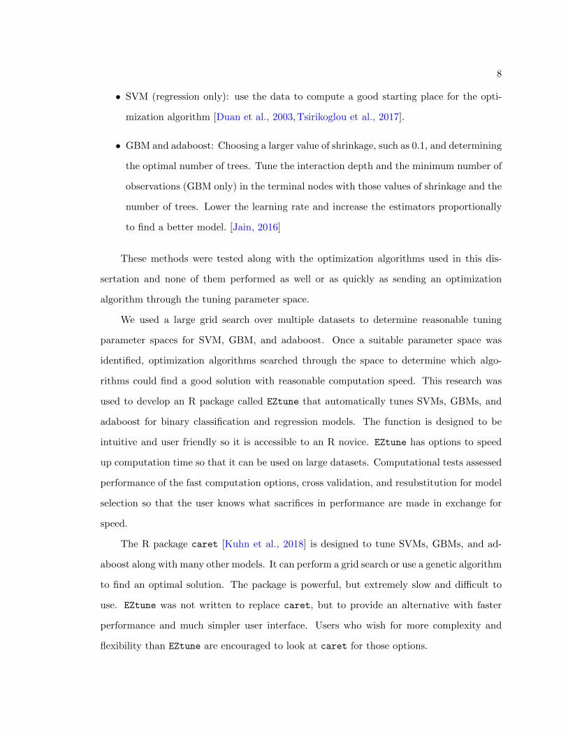
• GBM and adaboost: Choosing a larger value of shrinkage, such as 0.1, and determining
the optimal number of trees. Tune the interaction depth and the minimum number of
observations (GBM only) in the terminal nodes with those values of shrinkage and the
number of trees. Lower the learning rate and increase the estimators proportionally
to find a better model. [Jain, 2016]
These methods were tested along with the optimization algorithms used in this dis-
sertation and none of them performed as well or as quickly as sending an optimization
algorithm through the tuning parameter space.
We used a large grid search over multiple datasets to determine reasonable tuning
parameter spaces for SVM, GBM, and adaboost. Once a suitable parameter space was
identified, optimization algorithms searched through the space to determine which algo-
rithms could find a good solution with reasonable computation speed. This research was
used to develop an R package called EZtune that automatically tunes SVMs, GBMs, and
adaboost for binary classification and regression models. The function is designed to be
intuitive and user friendly so it is accessible to an R novice. EZtune has options to speed
up computation time so that it can be used on large datasets. Computational tests assessed
performance of the fast computation options, cross validation, and resubstitution for model
selection so that the user knows what sacrifices in performance are made in exchange for
speed.
The R package caret [Kuhn et al., 2018] is designed to tune SVMs, GBMs, and ad-
aboost along with many other models. It can perform a grid search or use a genetic algorithm
to find an optimal solution. The package is powerful, but extremely slow and difficult to
use. EZtune was not written to replace caret, but to provide an alternative with faster
performance and much simpler user interface. Users who wish for more complexity and
flexibility than EZtune are encouraged to look at caret for those options.

9
1.3.1 Genome-Wide Association Study Literature Review and Background
GWAS have been done since the early 2000s. The study done by the Wellcome Trust
Case Control Consortium (WTCCC) in 2007 [Wellcome Trust Case Control Consortium,
2007] was one of the first large scale GWAS. A GWAS looks for genetic variants that
are associated with a trait, or phenotype. The genetic variation is searched for in single
nucleotide polymorphisms (SNPs) which are single base pairs where genetic variation is
known to occur. GWAS data are ultra-high dimensional and can consist of hundreds of
thousands, or even millions, of SNPs that must be analyzed. A SNP is a single base pair
where genetic variation occurs. It is estimated that there are approximately 10 million
SNPs along the human genome. Breakthroughs in genetic technology have lead to an
increase in the number of genomes that can be sequenced for these analyses, but the large
number of SNPs results in a massive n<<p problem even with the increase in subjects.
Genetic properties such as linkage disequilibrium (LD) complicate statistical analysis. Many
methods have been used to conduct GWAS and development is ongoing as researchers
address the problems associated with data of this magnitude and complexity. This section
is not intended to list a comprehensive set of methods used to do GWAS, but rather it
introduces methods that inspired the method used in this dissertation.
Simple methods, such as logistic and linear regression, have been used to identify SNPs
associated with a trait, or phenotype. These models cannot be used on the entire dataset
because of the n<<p issue. A common method is to use single SNP regression [Wellcome
Trust Case Control Consortium, 2007]. This is where p regressions are done using the
phenotype as the response variable and a single SNP as the predictor. The p-values for the
coefficient are examined and SNPs with the smallest p-values are considered associated with
the phenotype. A similar method is implemented using distance correlation [Szekely et al.,
2007] where SNPs with a larger distance correlation with the phenotype are considered
associated with the trait. The Cochran-Armitage trend test [Freidlin et al., 2002] and χ2
statistic [Zeng et al., 2015] have also been extensively used for single SNP scans. Multiple
hypothesis testing is an issue that has been addressed in statistics for many years and several

10
methods for adjusting p-values have been developed to address this issue, but GWAS often
have at least tens of thousands, if not millions, of p-values to address. Existing methods
such as the Bonferroni correction [Perneger, 1998] are not equipped to handle so many tests.
Other methods such as the false discovery rate (FDR) [Benjamini and Hochberg, 1995] are
more appropriate, but still have limitations and best practices are not established [Wellcome
Trust Case Control Consortium, 2007]. Research is ongoing on how to handle the large
number of multiple tests.
LD poses other complications with single SNP scan methods. Neighboring SNPs are
typically highly correlated with each other and if a SNP is associated with the phenotype,
nearby SNPs that are not associated will have significant results because of their correlation
to the associated SNP. Conditional logistic regression has been used to correct for the effect
of LD in these situations. Conditional logistic regression repeats the single SNP logistic
regression for the SNPs that appear to be associated, but adds in the most significant
SNP as a covariate to correct for its effect. The p-value on the coefficient for the SNP of
interest is examined and if its association with the phenotype is due to the SNP on which
it is conditioned the p-value will no longer be significant [Chen et al., 2011]. This method
addresses LD, but it is not clear where to set p-value thresholds.
LASSO and elastic net have also been used to identify associated SNPs. LASSO was
used first and has been applied to the entire genome. This is computationally difficult and
LASSO is not able to select more SNPs that the number of subjects in a study [Wu et al.,
2009]. Elastic net was used to address this issue because it appeared that LASSO may be
too restrictive in SNP selection [Waldmann et al., 2013]. Both methods select SNPs that
have non-zero coefficients to go through another phase of statistical analysis. A common
follow up method was to compute a linear or logistic regression model with the SNPs that
have non-zero coefficients, compute the FDR for the p-values on the coefficients, and select
SNPs with FDRs that are less than a specified value. This method has shown promise, but
is is difficult to tune and perform LASSO or elastic net on such large datasets and there is
no clear guidance on how to select a threshold for the FDR. Despite these difficulties, good

11
results have been seen with these methods [Wu et al., 2009].
The field is actively being pursued as researchers seek new tools and better understand-
ing of existing tools. We seek to better understand how some of these popular methods
relate to each other when heritability in simulated data is controlled to different levels seen
in nature. We explore the efficacy of regression and distance correlation to filter out noise
while retaining regions with associated SNPs under low and high levels of heritability. We
also examine LASSO and elastic net after the noise has been removed. Random forests
and CART are used to identify SNPs that are strongly associated with the phenotype while
using LASSO and elastic net to identify SNPs that are less strongly correlated with the re-
sponse. The methods were evaluated using simulated data and an R package called gwas3
was created to implement the method and simulate GWAS data for study.

CHAPTER 2
TUNING SUPERVISED LEARNING METHODS
2.1 Introduction
In this chapter, we explore tuning parameters for SVMs, GBMs, and adaboost to
determine which parameters need tuning, determine a practical parameter space for each
model type, and explore optimization algorithms for searching over the parameter space.
This was done by identifying all of the tuning parameters for each model type and then
doing a large grid search for several datasets using each tuning parameter. The parameter
surface for each grid was examined for trends in model performance and computation speed.
Model performance was measured using error rate for binary classification models and MSE
for regression models. A parameter space was identified by this method which was then
searched by several optimization algorithms to find a set of parameters that resulted in a
good model. The results of this analysis were used to create an R package called EZtune
that is available on CRAN [R Core Team, 2019] which is discussed in chapter 3.
2.2 Optimization Algorithms
Optimization is a critical tool in machine learning and many algorithms have been
developed to perform this task. A large family of optimization algorithms look at the
neighborhood of the location of a point and determine a direction where the function value
is decreasing the most according to a certain criterion. Then, another point is chosen in the
decreasing direction and the process is repeated. Gradient based methods use the gradient
to determine which direction to go, but other algorithms may use a simplex or a line search
to determine which direction to travel. These methods can be very effective, but they also
run the risk of finding local minima and failing to find the global minimum. This has been
addressed by adding stochastic methods to some of the optimization algorithms. Other

13
methods use a completely different strategy to find an optimal solution. Genetic algorithms
use the idea of natural selection. Many points on the surface are tested and the best results
are kept as ”parents” to create optimal offspring. The concepts of mutation and breeding
introduce changes into the search so that the best solutions are not overlooked. Metaheuris-
tic algorithms, or nature inspired algorithms, use the behavior of natural organisms, such
as the swarming of bees or wolf hunting strategies, to devise a search method. Each of these
algorithm types work well in some situations and not well in others. We tried algorithms
from each of these areas to find tuning parameters for SVM, GBM, and adaboost that
minimize error measures.
2.3 Methods
Tuning parameters were assessed using six datasets with a binary response and seven
with a continuous response. Table 2.1 shows the datasets and their characteristics. Exten-
sive grid searchers were done with each dataset to determine a suitable tuning parameter
space. Then, a series of optimization algorithms were used to find a good set of tuning
parameters in that space. The results of each optimization algorithm were compared to the
best results that were found in the grid search. The error measure and computation time
were both considered when assessing the performance of the optimization algorithms.
2.3.1 Grid Search
Blog posts, books, and journal articles were read to explore the tuning parameter
ranges have been used by different sources. The parameter choice varies substantially for
each source. We used the widest range of parameters used by all of the sources we reviewed
and expanded some of them beyond what was seen in other sources. Table 2.2 shows the
ranges that were used for the grids. The results of the grid search indicate that the grids
were sufficiently large and did not need to be expanded beyond the limits in 2.2.
SVM, GBM, and adaboost models were computed throughout the grid region. The
error measure was evaluated at each grid location using 10-fold cross validation for most
datasets and and 3-fold cross validation for the largest datasets. The error measure is the

14
Tab
le2.
1:L
ist
ofd
atas
ets
use
dto
exp
lore
tun
ing
par
amet
ers.
Nu
mb
erof
Nu
mb
erof
Cat
egor
ical
Con
tinu
ous
Res
pon
seN
um
ber
ofN
um
ber
ofE
xp
lan
ator
yE
xp
lan
ator
yD
atase
tT
yp
eS
ourc
eO
bse
rvat
ion
sV
aria
ble
sV
aria
ble
sV
aria
ble
s
Bre
ast
Can
cer
Dat
aB
inary
mlb
ench
699
100
9[N
ewm
anet
al.,
1998
]Io
nos
ph
ere
Bin
ary
mlb
ench
351
341
33P
ima
Ind
ian
sB
inary
mlb
ench
768
90
8S
on
arB
inary
mlb
ench
208
610
60L
ich
enB
inary
EZ
tun
e84
034
231
[Lu
nd
ell,
2017
]M
ull
ein
Bin
ary
EZ
tun
e12
,094
320
31
Ab
alon
eR
egre
ssio
nA
pp
lied
Pre
dic
tive
Mod
elin
g4,
177
91
7[K
uh
nan
dJoh
nso
n,
2018
]B
osto
nH
ou
sin
g2
Reg
ress
ion
mlb
ench
506
171
15C
O2
Reg
ress
ion
dat
aset
s84
53
1[R
Cor
eT
eam
,20
19]
Cri
me
Reg
ress
ion
Ku
iper
4714
112
[Ku
iper
and
Skla
r,20
13]
Oh
ioH
ou
sin
gR
egre
ssio
nK
aggl
e1,
460
6136
24[D
eC
ock
,20
11,K
aggl
e,20
19]
Un
ion
Reg
ress
ion
Ku
iper
504
03
Wage
Reg
ress
ion
Ku
iper
3910
09
15
Table 2.2: List of tuning parameter ranges for grids.
Model Parameter Range
Support vector machine Cost [2−10, 225]γ [2−25, 210]
Gradient boosting machines Number of trees [50, 20,000]Interaction depth [1, 19]Shrinkage [0.001, 0.1]Minimum number of [5, 15]observations in terminal nodes
Adaboost Number of trees [100, 1400]Interaction depth [1, 20]Shrinkage (ν) [0.01, 1]
error rate for the binary data and the MSE for the continuous data. Computation time was
also recorded for each of the models. The surface of the error rates and MSEs across the
grid were examined for all datasets and models along with the computation time. A region
was found for all of the models that worked for all of the tested datasets. The regions
are identified in Section 2.4. Calculations were done using the packages e1071 [Meyer
et al., 2019], gbm [Greenwell et al., 2019], and ada [Culp et al., 2016] in the R statistical
software environment for statistical computing and graphics [R Core Team, 2019]. Note
that adaboost was not used on the regression datasets because the adaboost package that
was used does not have an option for regression data.
The stability of the models was of interest in this study. Error measures for each
fold of cross validation were used to compute a 95% upper confidence limit for the error
measures. This is because some learning models may provide results that are inconsistent.
The confidence limits were graphed and assessed for each grid location in addition to the
cross validated error measure and the computation time. In all cases, the surfaces produced
by the upper confidence limits yielded nearly identical surface patterns as the error measure
surfaces so they are not discussed further.
2.3.2 Optimization Algorithms
Once a parameter space was determined, the parameter spaces for each dataset were
searched by seventeen different optimization algorithms. Table 2.3 lists the algorithms with

16
a brief description of each one. Both the error measure and computation time were evaluated
for ten searches to determine the stability of the algorithm. If an algorithm was not able
to complete 10 runs within a specified time frame for one of the datasets, it was considered
a failure for that dataset. Different sizes of parameter spaces were tested if the grid search
surfaces indicated that there were multiple plausible parameter spaces. For example, the
error surface may show that a larger space is more likely to yield a good model than a
smaller space. However, the larger space may take too long to search.
The R statistical package [R Core Team, 2019] was used for all optimization computa-
tions. Table 2.4 shows the R packages and functions that were used. Computation time and
error measures were compared and it was assumed that different optimization algorithms
may perform better for different model types.
Table 2.3: List of optimization algorithms used to search tuning parameter spaces with abrief description of each method.
Algorithm Type Description
Ant Lion Metaheuristic Based on the hunting mechanisms
[Mirjalili, 2015a] of antlions
BOBYQA Derivative free Derivative free optimization by
[Powell, 2009] quadratic approximation
Dragonfly Metaheuristic Based on static and dynamic
[Mirjalili, 2016a] swarming behaviors of dragonflies
Firefly Metaheuristic Based on fireflies use of light to
[Yang, 2009] attract other fireflies
Genetic algorithm Metaheuristic Uses the principles of natural
[Goldberg, 1999] selection in successive generations
to find an optimal solution
Grasshopper Metaheuristic Mimics the behavior of
[Saremi et al., 2017] grasshopper swarms
Continued on next page

17
Table 2.3 – Continued from previous page
Algorithm Type Description
Grey wolf Metaheuristic Mimics leadership hierarchy
[Mirjalili et al., 2014] and hunting methods of grey wolves
Hooke-Jeeves Derivative free Pattern search that does a local
[Lai and Chan, 2007] search to find a direction where
performance improves and then
moves in that direction making
larger moves as long as
improvement continues
Improved harmony search Metaheuristic Mimics the improvisational
[Mahdavi et al., 2007] process of musicians
L-BFGS Quasi-Newton Second order method that
[Byrd et al., 1995] estimates the Hessian using
only recent gradients
Moth flame Metaheuristic Based on the navigation
[Mirjalili, 2015b] method of moths called
transverse orientation
Nelder-Mead Derivative free Direct search algorithm that
[Kelley, 1999] generates a simplex from sample
points, x, and uses
values of f(x) at the
vertices to search for an
optimal solution
Nonlinear conjugate Gradient The residual is replaced
gradient by a gradient and combined
[Dai and Yuan, 2001] with a line search method
Continued on next page

18
Table 2.3 – Continued from previous page
Algorithm Type Description
Particle swarm Metaheuristic Based on the evolutionary
[Shi and Eberhart, 1998] mechanisms that allows
organisms to adjust their flying
based on its own flying
experience and the experiences
of its companions
Sine cosine Metaheuristic Creates multiple initial random
[Mirjalili, 2016b] possible solutions and requires
them to fluctuate towards the
optimal solution using a
mathematical model based
on sine and cosine functions
Spectral projected Gradient Uses the spectrum of the
gradient underlying Hessian to
[Birgin et al., 2000] determine the step lengths
for gradient descent
Whale Metaheuristic Mimics the bubble-net
[Mirjalili and Lewis, 2016] hunting strategy of
humpback whales
2.4 Results
This section shows the results of the large grid search and the optimization tests. The
surfaces of the SVMs were smooth, but they were not smooth for either GBM or adaboost.
The tests showed that there are tuning parameter spaces that work for a wide choice of
datasets. Consistency was also found in optimization algorithm performance. Certain
optimization algorithms clearly outperformed the others.

19
Table 2.4: List of optimization algorithms along with the packages and functions in R thatwill be used to implement them.
Algorithm Package Function
Antlion MetaheuristicOpt ALO[Septem Riza et al., 2017]
BOBYQA minqa [Bates et al., 2014] bobyqaDragonfly MetaheuristicOpt DAFirefly MetaheuristicOpt FFAGenetic algorithm GA [Scrucca, 2013] gaGrasshopper MetaheuristicOpt GOAGrey wolf MetaheuristicOpt GWOHooke-Jeeves optimx [Nash, 2014a], hjk,
dfoptim [Varadhan et al., 2018] hjkbImproved harmony search MetaheuristicOpt HSL-BFGS lbfgsb3 [Nash et al., 2015], lbfgsb3,
stats [R Core Team, 2019] optimMoth flame MetaheuristicOpt MFONelder-Mead dfoptim nmkNonlinear conjugate gradient Rcgmin [Nash, 2014b] RcgminParticle swarm MetaheuristicOpt PSOSine cosine MetaheuristicOpt SCASpectral projected gradient BB [Varadhan and Gilbert, 2009] spgWhale MetaheuristicOpt WOA

20
2.4.1 Results of Grid Search
Grid searches were done using the data listed in Table 2.1 over the parameter ranges
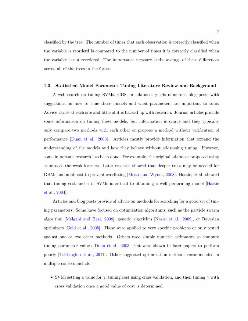
specified in Table 2.2. Figure 2.1 shows the surface of the errors obtained by the SVM
models for the six binary datasets. Although a distinct surface emerges across all of the
datasets, it is difficult to determine a smaller parameter area where performance is good
across all datasets. The grid results were subsetted to include only best 20% of the errors
and to include the best 20 error rates across the entire grid. Figure 2.2 shows the surface
for the computation times across the grid with the fastest 20 computation times highlighted
in orange.
The wide distribution of the orange dots in Figures 2.1 and 2.2 shows that there are
many local minima across the surface. Figure 2.2 also shows that there are areas in this
region that likely have slow computation time. The best computation times seemed to be
in the same grid regions with the best error rates. The MSE and computation time surfaces
for the regression datasets were similar to those for the binary data. Smaller values of ε
produced smaller MSEs but also had slower computation times for all datasets. Good error
rates with reasonable computation times can be obtained by models with a cost between 1
and 1000 and a γ between 2−10 to 210. The best results for regression were seen for values of
ε less than 0.5. It is clear from the analysis that cost, γ, and ε should all be tuned. Although
the regression and binary datasets showed similar results, the parameter spaces selected for
data types are slightly different. This is so the subtle differences between each model type
can be best utilized. Tables 2.5 and 2.6 show the selected tuning parameter spaces for all
of the models. Starting values for each of the parameter spaces were also selected from the
error surfaces. The starting locations were selected from areas that tend to have low error
measures and faster computation times across all datasets.
GBM was searched in a similar manner. The regression and binary plots showed the
same patterns although none of the error rate or computation time surfaces were smooth,
even when examined with multidimensional graphics. Computation times were unilater-
ally faster with smaller values for all tuning parameters with the exception of shrinkage.

21
Mullein Pima Sonar
Breast Cancer Ionosphere Lichen
−10 0 10 20 −10 0 10 20 −10 0 10 20
−20
−10
0
10
−20
−10
0
10
Cost ( 2x )
γ ( 2
y )
0.1
0.2
0.3
0.4
0.5
Error
All Errors for SVM Binary Data
●●
● ●●
●● ● ●●●
●●
●●●●
●●●
●●● ●●
●●●
●●
● ● ●● ● ●●
●● ●
●●
●
● ●●●
●● ●
●●
●●
●
●● ● ●
●
●
●
●
●
●
●
●
●
●
●●
● ●●
●
●
●
●
●
●
●
●●
●
●●●
●
●
●●
●
●●
●●
●●
●●
●● ● ●● ● ● ●●
● ●● ●●
● ●●
●
● ●
Mullein Pima Sonar
Breast Cancer Ionosphere Lichen
−10 0 10 20 −10 0 10 20 −10 0 10 20
−20
−10
0
10
−20
−10
0
10
Cost ( 2x )
γ ( 2
y )
0.05
0.10
0.15
0.20
Error
Best 20% Errors for SVM Binary Data with 20 Best Highlighted
Fig. 2.1: Error surface plots for support vector machines on datasets with a binary response.The orange dots on the bottom figure represent the best 20 models across the grid.

22
●● ●●●
●
●
●●
●
●
●
●
●●
●
●
●
●
●
Breast Cancer
−10 0 10 20
−20
−10
0
10
Cost ( 2x )
γ ( 2
y )
2
4
6
Time
Breast Cancer Time Surface
●
●●●
●●●● ● ●●
● ●●●●● ● ● ●
Ionosphere
−10 0 10 20
−20
−10
0
10
Cost ( 2x )
γ ( 2
y )
10
20
30
40
50
Time
Ionosphere Time Surface
●●●
●●
● ●
●
●
●
●
●
●● ●
●●
●
●
●
Lichen
−10 0 10 20
−20
−10
0
10
Cost ( 2x )
γ ( 2
y )
1000
2000
3000
Time
Lichen Time Surface
●●●
●●
●
●●
●
●
●
●
●
●●●
●●
●
●
Mullein
−10 0 10 20
−20
−10
0
10
Cost ( 2x )
γ ( 2
y )
1000
2000
3000
4000
Time
Mullein Time Surface
●●
●
●
●
●●●
●
●●
●●
●
●
●
●
●
●
●
Pima
−10 0 10 20
−20
−10
0
10
Cost ( 2x )
γ ( 2
y )
250
500
750
Time
Pima Time Surface
●●
●
●
●
●●
●
●
●
●
● ●
●●
●●
●●
●
Sonar
−10 0 10 20
−20
−10
0
10
Cost ( 2x )
γ ( 2
y )
0.5
1.0
Time
Sonar Time Surface
Fig. 2.2: Computation time surface plots for support vector machines on datasets with abinary response. The orange dots represent the 20 models with the shortest computationtimes across the grid. Time is in seconds.
Table 2.5: List of recommended tuning parameter spaces for binary classification modelsbased on grid search.
Model Parameter Ranges Start
SVM Cost [1, 1024] 10γ [2−10, 210] 2−5
GBM Num trees [50, 3000] 500Tree depth [1, 15] 5Shrinkage [0.001, 0.1] 0.1Min obs [5, 12] 8
Adaboost Num trees [50, 500] 300Tree depth [1, 10] 10Shrinkage [0.01, 0.5] 0.05
Surprisingly, shrinkage did not have much impact on computation time. The best error
measures were found across the range of shrinkage values, so a smaller shrinkage does not
always result in a better model. Better error rates were also found when fewer than 1000

23
Table 2.6: List of recommended tuning parameter spaces for regression models based ongrid search.
Model Parameter Ranges Start
SVM Cost [1, 1024] 2γ [2−10, 20] 2−5
ε [0, 0.5] 0.4
GBM Num trees [50, 5000] 2000Tree depth [1, 15] 8Shrinkage [0.001, 0.1] 0.1Min obs [5, 10] 5
iterations were done and often for only about 500 iterations. Good results were seen across
the spectrum of tested interaction depths and the different values of the minimum number
of observations in the terminal nodes that were tested. The areas of best performance var-
ied for each dataset so it was determined that the range of values should not be trimmed
much for those two tuning parameters. As with the SVM analysis, it was clear that it is
important to tune all four tuning parameters. Tables 2.5 and 2.6 show the selected tuning
parameter spaces.
Adaboost was assessed only for the binary datasets. The best computation times were
seen for the smallest number of trees and the smallest tree depths. Shrinkage did not have
much impact on computation times. Good error rates were seen across all values of shrinkage
that were tested and good models were found for all values of tree depth and the number
of iterations. The tuning parameter space was chosen to try to minimize computation time
while catching some of the best models for each dataset. Table 2.5 shows the selected tuning
parameter spaces.
Smaller regions than those listed in Tables 2.5 and 2.6 were tested during the opti-
mization phase to determine if reducing this region to a smaller area improves computation
time with little sacrifice in accuracy. It was found that smaller regions did not decrease
computation times for most optimization algorithms and often resulted in an increase in
error measure so the larger parameter space was retained.

24
2.4.2 Results of Optimization Algorithms
The optimization algorithms listed in Table 2.4 differed markedly in computation time
and in their ability to find a set of parameters that produced a good model. It was initially
thought that a gradient method would perform well for the SVM models because the error
surfaces were smooth and that non-gradient based algorithms would be better for GBM
and adaboost. The gradient based methods performed poorly for all models. The Hooke-
Jeeves algorithm consistently produced the best error measures and computation times
for all datasets across all model types. The genetic algorithm found the best error rates
overall, but computation times were slow. With larger datasets the computation time of
the genetic algorithm was prohibitive. Table 2.7 concisely summarizes the results of all of
the optimization algorithms. Figures 2.3 - 2.7 show parallel coordinate plots of the results
of the optimization tests. The times in the plots have been standardized by subtracting
the best error measure obtained from the grid search and then dividing by the maximum
resulting value. This means that the largest error measure for each dataset is expressed
by 1 and the best error measure seen in the grid search for a dataset is at 0. The time
plots were standardized by subtracting the fastest computation time from the optimization
tests from all of the times for each dataset and then dividing all of the resulting values by
the maximum. This means the slowest time for each dataset is represented by 1 and the
fastest time is represented by 0. The x-axis lists the R function name to avoid confusion
for algorithms tested with more than one function.
Optimization algorithms had some interesting behaviors. The non-linear conjugate
gradient algorithm had a very fast computation time, but it failed to move from the starting
values it was given. This may be an artifact of the Rcgmin function that was used [Nash,
2014b], but it is a gradient based function and it is unlikely it will perform well regardless
of how it is coded. The Nelder-Meade algorithm had fast computation times and low
error rates that rivaled the Hooke-Jeeves algorithm, but it often failed to converge. It is
worth exploring this algorithm in another programming language, such as Python, to see
if more stable performance can be achieved. The metaheuristic algorithms seem like they

25
Table 2.7: Performance summary of optimization algorithms.
Method Error Time Consistency
Genetic algorithm Good Slow ConsistentHooke and Jeeves Varies Varies InconsistentHooke and Jeeves B Good Good ConsistentL-BFGS Good Good Crashes oftenNocedal-Morales Poor Slow ConsistentNonlinear conjugate gradient Poor Fast Stays at startBOBYQA Poor Fast ConsistentL-BFGS B Poor Fast ConsistentSpectral projected gradient Moderate to Poor Good to moderate InconsistentAnt lion Poor Moderate ConsistentDragonfly Poor Good ConsistentFirefly Poor Slow ConsistentGrasshopper Moderate Moderate InconsistentGrey wolf Poor Moderate InconsistentHarmony search Poor Moderate InconsistentMoth flame Poor Moderate InconsistentParticle swarm Poor Slow ConsistentSine cosine Poor Moderate InconsistentWhale optimization Poor Slow Consistent
would perform well based on the appearance of the error rate surfaces and based on the
performance of the genetic algorithm so further investigation in Python or another language
may yield better results.
2.5 Conclusions
A large grid search was done for both binary classification and regression models us-
ing SVM and GBM. A grid search was done for adaboost for binary classification. It was
found that there were tuning parameter spaces for across all of the tested datasets that
contained models with small error measures and fast computation times. Areas that have
fast computation times for the SVM models also had good error rates for binary classifica-
tion. Regression models with SVM showed that this was true for cost and γ, but not for
ε. Tuning parameter spaces for binary and regression models were similar, but a smaller
region for γ can be used when the response is continuous.

26
0.00
0.25
0.50
0.75
1.00
alo
boby
qa da ffa ga goa
gwo
hjkb hjn hs
lbfgs
b3 mfo
nmkb
optim ps
osc
asp
gwoa
Sta
ndar
dize
d M
SE
Standardized MSEs
0.00
0.25
0.50
0.75
1.00
alo
boby
qa da ffa ga goa
gwo
hjkb hjn hs
lbfgs
b3 mfo
nmkb
optim ps
osc
asp
gwoa
Sta
ndar
dize
d T
ime
Standardized Computation Time
Abalone
Boston Housing
CO2
Crime
Ohio Housing
Union
Wage
Fig. 2.3: Standardized optimization results for support vector machines for regression.
GBM and adaboost have nearly identical tuning parameters, but they behave differ-
ently. GBM requires a larger range of trees and interaction depths than adaboost. They
also have different shrinkage ranges. A smaller shrinkage was not always better and did not
seem to increase computation time.
Optimization searches through the parameter spaces consistently shows that the genetic
algorithm was able to find the best error measures, but computation times were very slow.
It also shows that the Hooke-Jeeves algorithm outperforms all other algorithms in terms
of computation time, stability, and error measure. The Nelder-Meade algorithm had good
performance in regard to error measures and computation time, but it was unstable and
often failed to converge. Gradient based methods did not work well for any of the tested
models.
27
0.00
0.25
0.50
0.75
1.00
alo
boby
qa da ffa ga goa
gwo
hjkb hjn hs
lbfgs
b3 mfo
optim ps
o
Rcgm
in sca
woa
Sta
ndar
dize
d M
SE
Standardized MSEs
0.00
0.25
0.50
0.75
1.00
alo
boby
qa da ffa ga goa
gwo
hjkb hjn hs
lbfgs
b3 mfo
optim ps
o
Rcgm
in sca
woa
Sta
ndar
dize
d T
ime
Standardized Computation Time
Abalone
Boston Housing
CO2
Crime
Ohio Housing
Union
Wage
Fig. 2.4: Standardized optimization results for gradient boosting machines for regression.

28
0.00
0.25
0.50
0.75
1.00
ALO
boby
qa DAFFA ga
GOAGW
Ohjk
b hjn HS
lbfgs
b3M
FOnm
kbop
tim PSO
Rcgm
inSCA
spg
two
WOA
Sta
ndar
dize
d E
rror
Standardized Errors
0.00
0.25
0.50
0.75
1.00
ALO
boby
qa DAFFA ga
GOAGW
Ohjk
b hjn HS
lbfgs
b3M
FOnm
kbop
tim PSO
Rcgm
inSCA
spg
two
WOA
Sta
ndar
dize
d T
ime
Standardized Computation Time
Breast Cancer
Ionosphere
Lichen
Mullein
Pima
Sonar
Fig. 2.5: Standardized optimization results for support vector machines for binary classifi-cation.

29
0.00
0.25
0.50
0.75
1.00
alo
boby
qa da ffa ga goa
gwo
hjkb hjn hs
lbfgs
b3 mfo
nmkb
optim ps
o
Rcgm
in sca
spg
woa
Sta
ndar
dize
d E
rror
Standardized Errors
0.00
0.25
0.50
0.75
1.00
alo
boby
qa da ffa ga goa
gwo
hjkb hjn hs
lbfgs
b3 mfo
nmkb
optim ps
o
Rcgm
in sca
spg
two
woa
Sta
ndar
dize
d T
ime
Standardized Computation Time
Breast Cancer
Ionosphere
Lichen
Mullein
Pima
Sonar
Fig. 2.6: Standardized optimization results for gradient boosting machines for binary clas-sification.

30
0.25
0.50
0.75
1.00
alo da ffa ga goa
gwo
hjkb hjn hs
lbfgs
b3 mfo
nmkb
optim ps
o
Rcgm
in sca
spg
woa
Sta
ndar
dize
d E
rror
Standardized Errors
0.00
0.25
0.50
0.75
1.00
alo da ffa ga goa
gwo
hjkb hjn hs
lbfgs
b3 mfo
nmkb
optim ps
o
Rcgm
in sca
spg
woa
Sta
ndar
dize
d T
ime
Standardized Computation Time
Breast Cancer
Ionosphere
Lichen
Mullein
Pima
Sonar
Fig. 2.7: Standardized optimization results for adaboost models for binary classification.

31
CHAPTER 3
EZTUNE: AN R PACKAGE FOR AUTOMATIC TUNING OF SUPPORT VECTOR
MACHINES, GRADIENT BOOSTING MACHINES, AND ADABOOST
3.1 Introduction
EZtune is an R package that incorporates the information on tuning and optimiza-
tion from Chapter 2 into a few functions that can automatically tune SVMs, GBMs, and
adaboost. The idea for the package came from frustration in trying to tune supervised
learning models and finding that available tools are slow and difficult to use [Kuhn et al.,
2018], have limited capability [Meyer et al., 2019], or are not reliably maintained. EZtune
was developed to be as easy to use off the shelf as random forests while providing the user
with well tuned models within a reasonable computation time. The primary function in
EZtune searches the parameter spaces outlined in Chapter 2 using either a Hooke-Jeeves or
genetic algorithm. Data with a binary or continuous response can be tuned.
EZtune is not the only R package that can tune statistical learning models. The
package e1071 has a function called tune.svm that can tune SVMs quickly [Meyer et al.,
2019]. In comparing EZtune with tune.svm it appears that tune.svm tunes by optimizing
resubstitution error rates or MSE with a BFGS-L optimization algorithm. Tests from the
previous chapter show that other algorithms can consistently find a better model than
BFGS-L. Tests in this chapter show that using resubstitution to optimize does not produce
good results relative to other methods. However, SVMs tuned using tune.svm perform well
and it is a helpful tool to R users working with SVMs. If one wishes to tune a GBM or
adaboost to compare performance to the SVM, the e1071 package does not provide any
tools. The leading package for GBMs is gbm [Greenwell et al., 2019] and for adaboost it is
ada [Culp et al., 2016]. Neither of these packages provide tools for automatic tuning.
The most common tool for model tuning in R is caret [Kuhn et al., 2018]. The

32
caret package is a powerful tool that can tune dozens of different model types using several
different methods. Options for grid search and optimized search with a genetic algorithm
are available. It can also examine variable importance to aid in feature selection and has
graphical tools available for the different capabilities of the package. It is a tool that is
invaluable to someone who does a great deal of model tuning and needs a vast selection of
options from their tuning tools. Because caret is so all-inclusive, it is extremely difficult to
use. The documentation is extensive, but because so many options exist the documentation
is often inadequate for a user trying to perform a specific task. It also requires the user
to know what parameter spaces should be tuned over. Unless a user is proficient and
knowledgeable with tuning, using caret effectively is a daunting and time consuming task
that is nearly impossible for newcomers to tuning. Tuning with caret is also a long process
due to slow computation times. EZtune is not designed to replace caret. The functionality
of EZtune is nowhere near as extensive as that of caret, but it is designed to provide
a powerful alternative that is more accessible to non-experts and provide options for fast
computation.
EZtune consists of two functions and four datasets. One function finds a tuned model
that performs well and the other function verifies the performance of that model using
cross validation. The function returns the model and information about the model that
the user may find helpful. The default settings are designed to find a well tuned model
with short computation time, but several arguments can be changed by the user if different
options are desired. The philosophy behind the package is to allow even novice users to
easily tune SVMs, GBMs, and adaboost for both binary classification and regression models
without having to do significant research prior to tuning. Because the package is written
using the research presented in Chapter 2, the package produces well tuned models within
reasonable computation time. The EZtune package presented in this dissertation is version
2.0.0. EZtune 1.0.0 has many of the same capabilities as version 2.0.0 except that it does
not fit regression models and it was not based on the research in Chapter 2 so it does not
perform as well as version 2.0.0 [Lundell, 2017].

33
3.2 Package Components and How to Use Them
EZtune consists of the functions eztune and eztune cv. One function finds a well
tuned model and the other provides a cross validated error or MSE for that model. Four
datasets are also included in the package.
3.2.1 Datasets
The datasets included in EZtune are the mullein, mullein test, lichen, and lichen test
datasets from the article Random Forests for Classification in Ecology [Cutler et al., 2007].
Both datasets are large for automatic tuning and were used as part of package development
to test performance and computation speed for large datasets.
Lichen Data
The lichen data consist of 840 observations and 40 variables. One variable is a location
identifier, 7 (coded as 0 and 1) identify the presence or absence of a type of lichen species,
and 32 are characteristics of the survey site where the data were collected. Data were
collected between 1993 and 1999 as part of the Lichen Air Quality surveys on public lands
in Oregon and southern Washington. Observations were obtained from 1-acre (0.4 ha)
plots at Current Vegetation Survey (CVS) sites. Indicator variables denote the presences
and absences of seven lichen species. Data for each sampled plot include the topographic
variables elevation, aspect, and slope; bioclimatic predictors including maximum, minimum,
daily, and average temperatures, relative humidity precipitation, evapotranspiration, and
vapor pressure; and vegetation variables including the average age of the dominant conifer
and percent conifer cover.
Twelve monthly values were recorded for each of the bioclimatic predictors in the
original dataset. Principal components analyses suggested that for each of these predictors
two principal components explained the vast majority (95.0%-99.5%) of the total variability.
Based on these analyses, indices were created for each set of bioclimatic predictors. These
variables were averaged into yearly measurements. Variables within the same season were
also combined and the difference between summer and winter averages were recorded to

34
provide summer to winter contrasts. The averages and differences are included in the data
in EZtune.
Lichen Test Data
The lichen test data consist of 300 observations and 40 variables. Data were collected
from half-acre plots at CVS sites in the same geographical region and contain many of
the same variables, including presences and absences for the seven lichen species. The 40
variables are the same as those for the lichen data and it is a good test dataset for predictive
methods applied to the Lichen Air Quality data.
Mullein Data
The mullein dataset consists of 12,094 observations and 32 variables. It contains infor-
mation about the presence and absence of common mullein (Verbascum thapsus) at Lava
Beds National Monument. The park was digitally divided into 30m × 30m pixels. Park
personnel provided data on 6,047 sites at which mullein was detected and treated between
2000 and 2005, and these data were augmented by 6,047 randomly selected pseudo-absences.
Measurements on elevation, aspect, slope, proximity to roads and trails, and interpolated
bioclimatic variables such as minimum, maximum, and average temperature, precipitation,
relative humidity, and evapotranspiration were recorded for each 30m × 30m site.
Twelve monthly values were recorded for each of the bioclimatic predictors in the
original dataset. Principal components analyses suggested that for each of these predictors
two principal components explained the vast majority (95.0%-99.5%) of the total variability.
Based on these analyses, indices were created for each set of bioclimatic predictors). These
variables were averaged into yearly measurements. Variables within the same season were
also combined and the difference between summer and winter averages were recorded to
provide summer to winter contrasts. The averages and differences are included in the data
in EZtune.

35
Mullein Test Data
The mullein test data consists of 1512 observations and 32 variables. One variable
identifies the presence or absence of mullein in a 30m × 30m site and 31 variables are
characteristics of the site where the data were collected. The data were collected in Lava
Beds National Monument in 2006 that can be used to verify evaluate predictive statistical
procedures applied to the mullein dataset.
3.2.2 Automatic Tuning with eztune
The eztune function is the primary function in the EZtune package. The only required
arguments are the predictors and the response variable. The function is built on existing R
packages that are well maintained and well programmed to ensure that eztune performance
is reliable. SVM models are computed using the e1071 [Meyer et al., 2019], GBMs with
the gbm package [Greenwell et al., 2019], and adaboost with the ada package [Culp et al.,
2016]. The models produced by eztune are objects from each of these packages so all of
the peripheral functions for these packages can be used on models returned by eztune. A
summary of each of these packages and why they were chosen follows.
e1071 Package for Support Vector Machines
The e1071 package was written and is maintained by David Meyer [Meyer et al., 2019].
The package was built using the LIBSVM platform [Chang and Lin, 2011], which is written
in C++ and is considered one of the best open source libraries for SVMs. e1071 has been
around for many years and has continuously been updated during that time frame. It has
all of the features needed to perform the tasks needed by eztune and includes other features
that allow expansion of eztune in future versions, such as selection of kernels other than
the radial kernel and multi-class modeling.
gbm Package for Gradient Boosting Machines
The gbm package was written by Greg Ridgeway [Greenwell et al., 2019] and has been
maintained and updated for many years. It performs GBM by using the framework of an

36
adaboost model with an exponential loss function, but uses Friedman’s gradient descent
algorithm [Friedman, 2001] to optimize the trees rather than the algorithm originally pro-
posed in adaboost [Freund and Schapire, 1997]. This package was selected because it had all
of the features needed for eztune and included the ability to compute a multi-class model
for future EZtune versions.
ada Package for Adaboost Implementation
In contrast to SVMs and GBMs, there are several standard packages in R that can be
used to fit adaboost models. The most established and well known package is ada [Culp
et al., 2016]. Other packages that are often used are fastAdaboost [Chatterjee, 2016] and
adabag [Alfaro et al., 2013]. fastAdaboost is a new package with a fast implementation of
adaboost that is quickly gaining popularity. However, it is still being developed and does
not have all of the functionality needed for eztune. It may be considered as a platform
for later versions of eztune as fastAdaboost gains more functionality because adaboost
is currently the slowest model to tune. The package adabag provides an implementation
of adaboost that allows for bagging to be incorporated. This feature is useful, but it does
not allow for independent tuning of shrinkage or tree depth. Because these parameters
are important tuning parameters, adabag was not considered. The ada package has been
maintained and updated consistently for many years and had the capability to tune the
number of trees, tree depth, and shrinkage independently. Thus, ada was chosen as the
primary adaboost package for eztune.
Implementation of eztune
The eztune function was designed to be easy to use. It can be used when only data
are provided, but arguments can be changed for user flexibility. The default settings were
chosen to provide fast implementation of the function with good error rates. The syntax is:
eztune(x, y, method = "svm", optimizer = "hjn", fast = TRUE, cross = NULL)
Arguments:

37
• x: matrix or data frame of dependent variables.
• y: numeric vector of responses.
• method: ”svm” for SVMs, ”ada” for adaboost, and ”gbm” for GBMs.
• optimizer: ”hjn” for Hooke-Jeeves algorithm or ”ga” for genetic algorithm.
• fast: Indicates if the function should use a subset of the observations when optimizing
to speed up calculation time. Options include TRUE, a number between 0 and 1, and
a positive integer. A value of TRUE will use the smaller of 50% of the data or 200
observations for model fitting. A number between 0 and 1 specifies the proportion
of data that will be used to fit the model. A positive integer specifies the number of
observations that will be used to fit the model. A model is computed using a random
selection of data and the remaining data are used to validate model performance.
Validation error rate or MSE is used as the optimization measure.
• cross: If an integer k>1 is specified, k-fold cross validation is used to fit the model.
This parameter is ignored unless fast = FALSE.
The function determines if a response is binary or continuous and then performs the
appropriate grid search based on the function arguments. Testing showed that the SVM
model is faster to tune than GBMs and adaboost, with adaboost being substantially slower
than either of the other models. Tuning is also very slow as datasets get large. The mullein
and lichen datasets in this package tune very slowly because of their size. This is why the
fast options are set as the default. If a user wants a more accurate model and is willing
to wait for it, they can select cross validation or fit with a larger subset of the data. The
performance of the optimization algorithm features is presented in Section 3.3.
The Hooke-Jeeves optimization algorithm was chosen as the default optimization tool
because it outperformed all of the other algorithms tested in Table 2.4 in terms of speed
and finding an optimal model for all data and model types. It did not always produce the
best model out of the algorithms, but it was the only algorithm that was always among the

38
best performers. The only other algorithm that consistently produced models with error
measures as low or lower than those found by the Hooke-Jeeves algorithm were those found
by the genetic algorithm. The genetic algorithm was able to find a much better model than
Hooke-Jeeves in some situations, so it is included in the package. However, computation
time for the genetic algorithm is very slow, particularly for large datasets. If a user is in
need of a more accurate model and can wait for a longer computation time, the genetic
algorithm is worth trying. However, eztune will typically produce a very good model using
the Hooke-Jeeves option with a much faster computation time. The function hjn from
the optimx package [Nash, 2014a] is used to implement the Hooke-Jeeves algorithm. The
package dfoptim has a function called hjkb that also performs the Hooke-Jeeves algorithm,
but tests show that the hjn function performs better and more consistently than hjkb.
Several packages in R will implement a genetic algorithm, but the package GA is the most
comprehensive and best maintained genetic algorithm package on CRAN so it is used for
genetic algorithm optimization in eztune.
The fast options were chosen to allow the user to adjust computation time for different
dataset sizes. The default setting will use 50% of the data for datasets with less than 400
observations. If the data have more than 400 observations, 200 observations are chosen
at random as training data and the remaining data are used for model verification. This
options allows for very large datasets to be tuned quickly while ensuring there is a sufficient
amount of verification data for smaller datasets. The user can change these setting to meet
the needs of their project and accommodate their dataset. For example, 200 observations
may not be enough to tune a model for a dataset as large as the mullein dataset. The user
can increase that number of observations used to train the model using the fast argument.
The function returns a model and numerical measures that are associated with the
model. The model that is returned is an object from the package used to create the model.
The SVM model is of class svm, the GBM model is of class gbm.object, and the adaboost
model is of class ada. These models can be used with any of the features and functions
available for those objects. The accuracy and MSE is returned as well as the final tuning

39
parameters. The names of the parameters match the names from the function used to
generate them. For example, the number of trees used in gbm is called n.trees while the
same parameter is called iter for adaboost. This may seem confusing, but it was anticipated
that users may want to use the functionality of the e1071, gbm, and ada packages and naming
the parameters to match those packages will make moving from EZtune to the other packages
easier. If the fast option is used, eztune will return the number of observations used to
train the dataset. If cross validation is used, the function will return the number of folds
used for cross validation.
3.2.3 Model Performance Verification with eztune cv
Because eztune has many options for model optimization, a second function is in-
cluded to assess model performance using cross validation. It is known that model accuracy
measures based on resubstitution are overly optimistic. That is, when the data that were
used to create the model are used to verify the model, model performance will typically
look much better than it actually is. Fast options in eztune use data splitting so that
the models are optimized using verification data rather than training data. However, the
training dataset may be a small fraction of the original dataset to decrease computational
speed which may result in a model that is not as accurate as desired.
The function eztune cv was developed to easily verify a model computed by eztune
using cross validation so that a better estimate of model accuracy can be quickly obtained.
The predictors and response are inputs into the function along with the object obtained
from eztune. The eztune cv function returns a number that represents the cross validated
accuracy or MSE. Function syntax is:
eztune cv(x, y, model, cross = 10)
Arguments:
• x: Matrix or data frame of dependent variables.
• y: Numeric vector of responses.

40
• model: Object generated with the function eztune.
• cross: The number of folds for n-fold cross validation.
The function returns a numeric value that represents the cross validated accuracy of the
model.
3.3 Performance and Benchmarking
Tests were performed on the thirteen datasets listed in Table 2.1. Because a large
grid search was done for each of the datasets using all of the model types, results of the
package tests were compared to the best error rates and MSEs obtained from the grid
search. Computation times are also reported for all runs so that computation time and
model performance can be balanced by the user. Each of the tests were run 10 times so
that the stability of model results and test times could be assessed. Figures 3.1 - 3.5 show
the performance of the function for different argument inputs. The lines represent the
standardized cross validated MSEs or error rates for each of the model types and datasets.
For each dataset, the data were rescaled so that the largest MSE or error rate achieved by
a model type is represented by a 1 and the smallest MSE or error rate is represented by
a 0. The same standardization was done for computation time. Thus, results are directly
comparable for all results obtained for a dataset with a specific model type. Tables 3.1 -
3.5 show the mean cross validated MSEs and error rates for each run along with the mean
computation time in seconds. If a table entry is NA it means the computations could not
be completed because the dataset is too small for the argument setting. Note that ten
runs were not completed for some of the mullein genetic algorithm runs using 10-fold cross
validation because computation time was near 72 hours for that setting. However, at least
one run was obtained for each setting with mullein.
Both SVM and GBM regression results show that using resubstitution for optimization
is a poor choice. The MSEs obtained from resubstitution models are particularly bad for
SVMs, but are also consistently bad for GBMs. Computation time for this method is
also much slower than the fast options. Resubstitution also does not perform well for the

41
binary classifiers. It performs particularly poorly for the genetic algorithm with GBMs and
Hooke-Jeeves for adaboost. It is consistently the worst option for SVM for both optimization
algorithms. It is also not faster than the fast options. Hence, it is not recommended to use
resubstitution for optimization.
Cross validation and the fast options give the best MSEs and error rates. Cross val-
idation with 10-folds seems to perform the best most often for SVM regression and clas-
sification. It is also the best performer for the genetic algorithm for GBM classification
and does well for regression. However, it is not particularly good for adaboost. Ten-fold
cross validation is the slowest way to optimize by a substantial amount. Three-fold cross
validation produces good results for most datasets with much faster computation time, but
it is still much slower than the fast options.
The fast options improve computation time unilaterally, as they are intended. The
default fast option, which is to use the lesser of 50% of the data or 200 observations,
performs as well as many of the other fast options except for the mullein dataset and for
Hooke-Jeeves with the Boston Housing dataset. For datasets that are larger, such as lichen,
mullein, and abalone, using a larger set of observations as the training data for the fast
option often improves model performance, but it is not always needed. The fast option
is a good place to start for a model and for moderately sized datasets the default setting
produces a good model. However, for larger datasets, it may be worth sacrificing some
computation time to get better model accuracy.
Tables 3.1 - 3.5 show the performance of the package in comparison to the best model
obtained from the grid search. Tables 3.1 and 3.2 show that smaller datasets have unstable
results, with MSEs varying more from the grid search results than for larger datasets. In
particular, the MSE for the wage data is far larger than the best MSE obtained from the
grid. The wide range of results indicates that the models are volatile. Larger datasets are
able to obtain MSEs that are close to the best results seen in the grids for many of the
options. Cross validation options and fast options produce the MSEs that are closest to the
best grid values. The largest dataset that was tested is the mullein dataset and it appears

42
that it is better to use a larger proportion of the data rather than a low fixed value, but the
computation time increases substantially. It is also clear from Table 3.5 that adaboost seems
to produce models with larger error measures than SVM and GBM and the computation
times are much longer than for SVM and GBM. This likely due to the different platforms
used to construct the package, but it may warrant further investigation on better ways to
implement adaboost. It is also clear from the tables that the cross validation options are
very slow for large datasets and 10-fold cross validation can take several days for datasets
as large as mullein.
Comparison of the Hooke-Jeeves algorithm to the genetic algorithms shows that one
does not consistently outperform the other. In most cases, the Hooke-Jeeves algorithm
produces slightly better results than the genetic algorithm, but there are cases where the
reverse is true. The computation time for the genetic algorithm is typically much longer
than for Hooke-Jeeves, particularly for regression and for larger datasets.
EZtune tests indicate that different arguments in the eztune function have a big impact
on the performance of the function. If a model with low error measures is desired, it is best
to use 10-fold cross validation or a fast option that uses over 50% of the data. Computation
times vary for each of the function options, but the best options in terms of computation
speed and performance seem to be the Hooke-Jeeves algorithm in conjunction with the fast
feature. For most datasets the fast=TRUE option provides a good model, but if the dataset
is large and greater computation time is feasible, using 50% or more of the data to train
yields very good results. The trials also show that for very small datasets, the results of
eztune are unstable. However, SVM, GBM, and adaboost are machine learning methods
and tend to perform better with larger datasets so this finding is not surprising.
3.4 Conclusions
EZtune is a package that was designed to tune supervised learning methods with a
simple user interface. It is built with existing R packages that are well maintained and have
been in used for several years. EZtune takes advantage of the strengths of these packages to
provide a function that can quickly find a good set of tuning parameters for SVM, GBM,
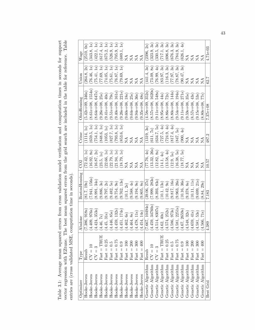
43
Tab
le3.
1:A
vera
ge
mea
nsq
uare
der
rors
from
cros
sva
lid
atio
nm
odel
veri
fica
tion
and
com
pu
tati
onti
mes
inse
con
ds
for
sup
por
tve
ctor
regr
essi
onw
ith
EZ
tun
e.T
he
bes
tm
ean
squ
ared
erro
rsfr
omth
egr
idse
arch
are
incl
ud
edin
the
tab
lefo
rre
fere
nce
.T
able
entr
ies
are
(cro
ssva
lid
ate
dM
SE
,co
mp
uta
tion
tim
ein
seco
nd
s).
Opti
miz
erT
yp
eA
balo
ne
Bost
onH
ousi
ng
CO
2C
rim
eO
hio
Hou
sing
Unio
nW
age
Hook
e-Jee
ves
Res
ub
(7.3
86,
918
s)(8
1.7,
19s)
(72.
42,
1s)
(111
4,1s)
(5.4
2e+
09,
346
s)(2
64.8
,2s
)(2
510,
0s)
Hook
e-Jee
ves
CV
=10
(4.4
09,
976
s)(7
.941
,156
s)(1
6.92
,8s
)(6
59.5
,1s
)(8
.61e+
08,
155
4s)
(76.
46,
1s)
(343
.8,
1s)
Hook
e-Jee
ves
CV
=3
(4.4
24,
353
s)(8
.991
,34s
)(1
6.87
,2s
)(7
54.1
,1s
)(8
.64e+
08,
647
s)(7
5.41
,1s
)(4
22.1
,1s
)H
ook
e-Jee
ves
Fast
=T
RU
E(4
.46,
7s)
(9.8
86,
3s)
(23.
5,1s
)(8
48.6
,1s
)(9
.26e+
08,
25s
)(7
7.69
,1s
)(6
17.4
,1s
)H
ook
e-Jee
ves
Fast
=0.
25(4
.45,
31s)
(9.7
97,
2s)
(22.
66,
1s)
(105
3,1s)
(9.4
1e+
08,
40s
)(7
4.05
,1s
)(6
75.2
,1s
)H
ook
e-Jee
ves
Fast
=0.
5(4
.446
,85s
)(9
.482
,5s)
(22.
79,
1s)
(827
.7,
1s)
(9.5
1e+
08,
79s
)(7
5.61
,1s
)(5
26.9
,1s
)H
ook
e-Jee
ves
Fast
=0.
75(4
.459
,132
s)(9
.754
,9s)
(21.
94,
1s)
(793
.8,
1s)
(9.4
0e+
08,
161
s)(7
6.87
,1s
)(7
05.9
,1s
)H
ook
e-Jee
ves
Fast
=0.
9(4
.451
,174
s)(9
.762
,13s
)(1
8.79
,1s
)(8
53.6
,1s
)(9
.26e+
08,
221
s)(7
9.69
,1s
)(6
89.1
,1s
)H
ook
e-Jee
ves
Fast
=10
0(4
.462
,6s)
(10.
1,2s
)N
AN
A(9
.60e+
08,
18s
)N
AN
AH
ook
e-Jee
ves
Fast
=20
0(4
.464
,8s)
(9.5
88,
4s)
NA
NA
(9.6
4e+
08,
25s
)N
AN
AH
ook
e-Jee
ves
Fast
=30
0(4
.478
,11s
)(9
.194
,9s)
NA
NA
(9.9
4e+
08,
36s
)N
AN
AH
ook
e-Jee
ves
Fast
=40
0(4
.454
,14s
)(9
.805
,8s)
NA
NA
(9.3
5e+
08,
48s
)N
AN
A
Gen
etic
Alg
ori
thm
Res
ub
(7.6
67,
104
94s)
(39.
06,
27s
)(7
7.76
,4s
)(1
319,
3s)
(4.5
8e+
09,
352
s)(4
41.4
,3s
)(2
396,
2s)
Gen
etic
Alg
ori
thm
CV
=10
(4.4
59,
347
60s)
(7.9
99,
283
s)(1
3.32
,26
s)(6
11,
7s)
(8.5
7e+
08,
162
0s)
(73.
09,
8s)
(323
.9,
3s)
Gen
etic
Alg
ori
thm
CV
=3
(4.5
14,
830
7s)
(8.3
93,
83s
)(1
2.82
,8s
)(6
34.7
,5s
)(9
.11e+
08,
548
s)(7
6.99
,4s
)(3
30.5
,3s
)G
enet
icA
lgori
thm
Fast
=T
RU
E(4
.62,
40s)
(10.
1,13
s)(1
4.1,
4s)
(727
.5,
4s)
(8.9
5e+
08,
44s
)(8
3.97
,3s
)(7
17.1
,3s
)G
enet
icA
lgori
thm
Fast
=0.
25(4
.574
,252
s)(1
0.42
,9s)
(13.
58,
4s)
(724
.9,
4s)
(8.8
6e+
08,
72s
)(1
16.3
,3s
)(6
96.8
,3s
)G
enet
icA
lgori
thm
Fast
=0.
5(4
.586
,973
s)(9
.817
,16s
)(1
2.9,
5s)
(817
.4,
4s)
(8.8
0e+
08,
144
s)(7
7.97
,3s
)(6
76.3
,3s
)G
enet
icA
lgori
thm
Fast
=0.
75(4
.581
,225
1s)
(9.9
63,
26s
)(1
6.38
,5s
)(8
47,
5s)
(9.5
4e+
08,
194
s)(7
8.87
,3s
)(7
84.9
,3s
)G
enet
icA
lgori
thm
Fast
=0.
9(4
.67,
2659
s)(1
0.16
,36s
)(1
8.77
,5s
)(9
00,
4s)
(9.1
1e+
08,
271
s)(9
0.47
,3s
)(6
26.1
,4s
)G
enet
icA
lgori
thm
Fast
=10
0(4
.548
,32s
)(9
.378
,8s)
NA
NA
(9.5
9e+
08,
35s
)N
AN
AG
enet
icA
lgori
thm
Fast
=20
0(4
.659
,41s
)(1
0.11
,11s
)N
AN
A(8
.57e+
08,
43s
)N
AN
AG
enet
icA
lgori
thm
Fast
=30
0(4
.581
,53s
)(9
.699
,21s
)N
AN
A(9
.15e+
08,
53s
)N
AN
AG
enet
icA
lgori
thm
Fast
=40
0(4
.566
,71s
)(8
.84,
29s)
NA
NA
(8.8
0e+
08,
77s
)N
AN
A
Bes
tG
rid
4.3
897.
183
10.5
748
7.2
7.37
e+08
62.
74.7
1e-0
3

44
Hooke−Jeeves
Genetic Algorithm
0.00
0.25
0.50
0.75
1.00
0.00
0.25
0.50
0.75
1.00
Sta
ndar
dize
d M
SE
Support Vector Regression
Abalone
BostonHousing
CO2
Crime
OhioHousing
Union
Wage
Hooke−Jeeves
Genetic Algorithm
Resub
CV = 1
0
CV = 3
Fast
= TRUE
Fast
= 0.
25
Fast
= 0.
5
Fast
= 0.
75
Fast
= 0.
9
Fast
= 10
0
Fast
= 20
0
Fast
= 30
0
Fast
= 40
0
0.00
0.25
0.50
0.75
1.00
0.00
0.25
0.50
0.75
1.00
Sta
ndar
dize
d T
ime
Fig. 3.1: Standardized mean squared error results and computation times for support vectorregression. The best mean squared errors and computation times for each dataset have avalue of 0 and the worst have a value of 1.

45
Tab
le3.2
:A
vera
ge
mea
nsq
uar
eder
rors
from
cros
sva
lid
atio
nm
od
elve
rifi
cati
onan
dco
mp
uta
tion
tim
esin
seco
nd
sfo
rgr
adie
nt
boos
ting
regre
ssio
nw
ith
EZ
tun
e.T
he
bes
tm
ean
squ
ared
erro
rsfr
omth
egr
idse
arch
are
incl
uded
inth
eta
ble
for
refe
ren
ce.
Tab
leen
trie
sar
e(c
ross
vali
date
dM
SE
,co
mp
uta
tion
tim
ein
seco
nd
s).
Opti
miz
erT
yp
eA
bal
one
Bos
tonH
ousi
ng
CO
2C
rim
eO
hio
Hou
sing
Unio
nW
age
Hook
e-Jee
ves
Res
ub
(5.6
59,
1832
s)(8
.036
,46
8s)
(8.4
09,
13s)
(570
.7,
13s)
(7.6
3e+
08,
4154s
)(1
31.4
,5s)
(2201
,4s)
Hook
e-Jee
ves
CV
=10
(4.5
88,
1136
6s)
(7.8
21,
2657
s)(5
.281
,10
3s)
(580
.2,
102s
)(7
.15e
+08
,22
685
s)(9
4.73,
37s
)(1
455
,39s)
Hook
e-Jee
ves
CV
=3
(4.5
79,
2515
s)(7
.664
,66
8s)
(6.5
67,
25s)
(550
.4,
20s)
(6.9
2e+
08,
5539s
)(9
6.38,
8s)
NA
Hook
e-Jee
ves
Fast
=T
RU
E(4
.961
,16
3s)
(8.4
7,14
4s)
(7.1
74,
6s)
(572
.8,
5s)
(7.1
8e+
08,
527s)
(94.
61,
2s)
NA
Hook
e-Jee
ves
Fast
=0.
25(4
.721
,42
3s)
(7.8
89,
90s)
(5.5
05,
1s)
(569
.8,
1s)
(6.6
7e+
08,
794s)
(107
.1,
0s)
NA
Hook
e-Jee
ves
Fast
=0.
5(4
.573
,70
6s)
(7.8
78,
167s
)(7
.017
,6s
)(6
45.6
,5s
)(6
.74e
+08
,15
77s
)(9
8.26,
2s)
NA
Hook
e-Jee
ves
Fast
=0.
75(4
.583
,88
1s)
(8.2
06,
253s
)(5
.355
,10
s)(6
28.4
,8s
)(7
.09e
+08
,19
07s
)(1
05.4
,3s)
NA
Hook
e-Jee
ves
Fast
=0.
9(4
.657
,11
93s)
(8.0
51,
322s
)(6
.248
,12
s)(6
07.4
,11
s)(7
.06e
+08
,25
34s
)(9
9.76,
4s)
(1744
,3s)
Hook
e-Jee
ves
Fast
=10
0(4
.928
,10
4s)
(7.9
23,
63s)
NA
NA
(7.0
3e+
08,
261s)
NA
NA
Hook
e-Jee
ves
Fast
=20
0(4
.947
,16
1s)
(8.1
31,
144s
)N
AN
A(7
.00e
+08
,51
9s)
NA
NA
Hook
e-Jee
ves
Fast
=30
0(5
.015
,18
2s)
(7.7
28,
209s
)N
AN
A(7
.26e
+08
,73
6s)
NA
NA
Hook
e-Jee
ves
Fast
=40
0(4
.97,
199
s)(8
.176
,25
3s)
NA
NA
(7.0
6e+
08,
981s)
NA
NA
Gen
etic
Alg
orit
hm
Res
ub
(5.7
78,
4067
s)(8
.082
,61
1s)
(9.2
86,
34s)
(594
.7,
20s)
(8.0
3e+
08,
5941s
)(1
33.2
,15s
)N
AG
enet
icA
lgor
ithm
CV
=10
(4.5
71,
1246
0s)
(7.9
87,
5843
s)(6
.343
,17
9s)
(570
.2,
194s
)(7
.00e
+08
,58
628
s)(9
9.73,
48s
)(1
751
,36s)
Gen
etic
Alg
orit
hm
CV
=3
(4.5
81,
3549
s)(7
.778
,13
98s)
(6.5
17,
53s)
(556
,42
s)(6
.58e
+08
,12
907
s)(1
11.3
,14s
)N
AG
enet
icA
lgor
ithm
Fast
=T
RU
E(4
.726
,20
9s)
(7.9
65,
259s
)(6
.882
,13
s)(5
80.7
,10
s)(7
.19e
+08
,92
7s)
(117
.5,
6s)
NA
Gen
etic
Alg
orit
hm
Fast
=0.
25(4
.588
,56
7s)
(8.0
97,
144s
)(7
.975
,2s
)N
A(6
.72e
+08
,16
49s
)(1
24.9
,2s)
NA
Gen
etic
Alg
orit
hm
Fast
=0.
5(4
.598
,10
98s)
(7.8
08,
419s
)(7
.059
,15
s)(5
44.5
,12
s)(7
.26e
+08
,27
80s
)(1
21.6
,4s)
NA
Gen
etic
Alg
orit
hm
Fast
=0.
75(4
.641
,14
89s)
(7.8
53,
447s
)(6
.758
,20
s)(5
73.4
,18
s)(7
.36e
+08
,52
29s
)(1
26.1
,9s)
NA
Gen
etic
Alg
orit
hm
Fast
=0.
9(4
.688
,18
14s)
(8.3
79,
538s
)(7
.084
,25
s)(5
80.7
,22
s)(7
.40e
+08
,44
33s
)(1
19.2
,10s
)(2
118
,7s)
Gen
etic
Alg
orit
hm
Fast
=10
0(4
.656
,16
9s)
(8.2
07,
113s
)N
AN
A(7
.10e
+08
,46
9s)
NA
NA
Gen
etic
Alg
orit
hm
Fast
=20
0(4
.69,
221
s)(7
.968
,32
6s)
NA
NA
(6.9
8e+
08,
1052s
)N
AN
AG
enet
icA
lgor
ithm
Fast
=30
0(4
.738
,27
3s)
(8.0
39,
484s
)N
AN
A(7
.24e
+08
,15
24s
)N
AN
AG
enet
icA
lgor
ithm
Fast
=40
0(4
.681
,30
3s)
(7.8
34,
603s
)N
AN
A(6
.86e
+08
,15
80s
)N
AN
A
Bes
tG
rid
4.44
26.
84.
568
391.
76.
04e+
0882
.86
0.0
262

46
Hooke−Jeeves
Genetic Algorithm
0.00
0.25
0.50
0.75
1.00
0.00
0.25
0.50
0.75
1.00
Sta
ndar
dize
d M
SE
Gradient Boosting Regression
Abalone
BostonHousing
CO2
Crime
OhioHousing
Union
Wage
Hooke−Jeeves
Genetic Algorithm
Resub
CV = 1
0
CV = 3
Fast
= TRUE
Fast
= 0.
25
Fast
= 0.
5
Fast
= 0.
75
Fast
= 0.
9
Fast
= 10
0
Fast
= 20
0
Fast
= 30
0
Fast
= 40
0
0.00
0.25
0.50
0.75
1.00
0.00
0.25
0.50
0.75
1.00
Sta
ndar
dize
d T
ime
Fig. 3.2: Standardized mean squared error results and computation times for gradientboosting regression. The best mean squared errors and computation times for each datasethave a value of 0 and the worst have a value of 1.

47
Tab
le3.3
:A
vera
gecl
assi
fica
tion
erro
rsfr
omcr
oss
vali
dat
ion
mod
elve
rifi
cati
onan
dco
mp
uta
tion
tim
esin
seco
nd
sfo
rsu
pp
ort
vect
orcl
ass
ifica
tion
wit
hE
Ztu
ne.
Th
eb
est
clas
sifi
cati
oner
rors
from
the
grid
sear
char
ein
clu
ded
inth
eta
ble
for
refe
ren
ce.
Tab
leen
trie
sare
(cro
ssva
lid
ated
erro
rra
te,
com
pu
tati
onti
me
inse
con
ds)
.
Op
tim
izer
Typ
eB
reas
tCan
cer
Ion
osp
her
eL
ich
enM
ull
ein
Pim
aS
onar
Hook
e-Jee
ves
Res
ub
(0.0
455,
2s)
(0.0
521,
2s)
(0.1
821,
11s)
(0.0
581,
6998
s)(0
.303
1,7s
)(0
.132
7,12
s)H
ook
e-Jee
ves
CV
=10
(0.0
312,
5s)
(0.0
544,
7s)
(0.1
446,
44s)
(0.0
574,
7013
0s)
(0.2
363,
26s)
(0.1
197,
48s)
Hook
e-Jee
ves
CV
=3
(0.0
338,
2s)
(0.0
587,
3s)
(0.1
538,
20s)
(0.0
575,
1882
7s)
(0.2
384,
10s)
(0.1
274,
26s)
Hook
e-Jee
ves
Fas
t=
TR
UE
(0.0
372,
1s)
(0.0
587,
2s)
(0.1
599,
4s)
(0.1
748,
70s)
(0.2
384,
1s)
(0.1
264,
15s)
Hook
e-Jee
ves
Fas
t=
0.25
(0.0
379,
1s)
(0.0
581,
2s)
(0.1
693,
3s)
(0.0
783,
539s
)(0
.239
3,1s
)(0
.127
4,13
s)H
ook
e-Jee
ves
Fas
t=
0.5
(0.0
401,
1s)
(0.0
57,
2s)
(0.1
64,
5s)
(0.0
581,
2745
s)(0
.233
6,3s
)(0
.126
4,15
s)H
ook
e-Jee
ves
Fas
t=
0.75
(0.0
379,
1s)
(0.0
55,
3s)
(0.1
705,
8s)
(0.0
576,
5128
s)(0
.253
4,4s
)(0
.129
8,17
s)H
ook
e-Jee
ves
Fas
t=
0.9
(0.0
397,
1s)
(0.0
544,
2s)
(0.1
681,
11s)
(0.0
681,
7179
s)(0
.243
6,5s
)(0
.130
8,19
s)H
ook
e-Jee
ves
Fas
t=
100
(0.0
391,
1s)
(0.0
524,
2s)
(0.1
623,
3s)
(0.1
645,
57s)
(0.2
374,
1s)
(0.1
25,
15s)
Hook
e-Jee
ves
Fas
t=
200
(0.0
351,
1s)
(0.0
553,
2s)
(0.1
74,
4s)
(0.1
69,
64s)
(0.2
43,
1s)
(0.1
298,
16s)
Hook
e-Jee
ves
Fas
t=
300
(0.0
365,
1s)
(0.0
524,
2s)
(0.1
6,5s
)(0
.162
7,70
s)(0
.241
7,2s
)N
AH
ook
e-Jee
ves
Fas
t=
400
(0.0
344,
1s)
NA
(0.1
582,
6s)
(0.1
563,
80s)
(0.2
435,
2s)
NA
Gen
etic
Alg
ori
thm
Res
ub
(0.0
53,
8s)
(0.1
598,
10s)
(0.2
098,
45s)
(0.0
578,
1306
4s)
(0.3
234,
25s)
(0.3
111,
58s)
Gen
etic
Alg
ori
thm
CV
=10
(0.0
321,
26s)
(0.0
481,
28s)
(0.1
496,
227s
)(0
.058
3,17
5904
s)(0
.230
2,24
8s)
(0.1
212,
176s
)G
enet
icA
lgori
thm
CV
=3
(0.0
327,
11s)
(0.0
55,
15s)
(0.1
494,
84s)
(0.0
587,
5853
1s)
(0.2
355,
72s)
(0.1
212,
105s
)G
enet
icA
lgori
thm
Fas
t=
TR
UE
(0.0
347,
5s)
(0.0
575,
9s)
(0.1
601,
14s)
(0.1
825,
137s
)(0
.232
2,8s
)(0
.126
9,80
s)G
enet
icA
lgori
thm
Fas
t=
0.25
(0.0
362,
4s)
(0.0
584,
8s)
(0.1
526,
15s)
(0.0
75,
1338
s)(0
.235
9,6s
)(0
.129
8,67
s)G
enet
icA
lgori
thm
Fas
t=
0.5
(0.0
329,
5s)
(0.0
581,
9s)
(0.1
487,
24s)
(0.0
608,
5163
s)(0
.237
1,15
s)(0
.126
,76
s)G
enet
icA
lgori
thm
Fas
t=
0.75
(0.0
378,
6s)
(0.0
601,
9s)
(0.1
606,
38s)
(0.0
587,
1360
4s)
(0.2
384,
25s)
(0.1
173,
76s)
Gen
etic
Alg
ori
thm
Fas
t=
0.9
(0.0
394,
6s)
(0.0
655,
8s)
(0.1
568,
41s)
(0.0
59,
1340
8s)
(0.2
44,
38s)
(0.1
212,
75s)
Gen
etic
Alg
ori
thm
Fas
t=
100
(0.0
397,
4s)
(0.0
604,
8s)
(0.1
662,
11s)
(0.1
898,
117s
)(0
.234
8,5s
)(0
.126
9,74
s)G
enet
icA
lgori
thm
Fas
t=
200
(0.0
354,
5s)
(0.0
621,
10s)
(0.1
539,
15s)
(0.1
813,
126s
)(0
.235
7,8s
)(0
.123
1,64
s)G
enet
icA
lgori
thm
Fas
t=
300
(0.0
359,
4s)
(0.0
644,
9s)
(0.1
551,
17s)
(0.1
786,
142s
)(0
.235
3,12
s)N
AG
enet
icA
lgori
thm
Fas
t=
400
(0.0
329,
6s)
NA
(0.1
515,
22s)
(0.1
709,
202s
)(0
.232
,15
s)N
A
Bes
tG
rid
0.02
340.
0427
0.13
10.
0682
0.21
740.
101

48
Hooke−Jeeves
Genetic Algorithm
0.00
0.25
0.50
0.75
1.00
0.00
0.25
0.50
0.75
1.00
Sta
ndar
dize
d E
rror
Rat
eSupport Vector Machine
BreastCancer
Ionosphere
Lichen
Mullein
Pima
Sonar
Hooke−Jeeves
Genetic Algorithm
Resub
CV = 1
0
CV = 3
Fast
= TRUE
Fast
= 0.
25
Fast
= 0.
5
Fast
= 0.
75
Fast
= 0.
9
Fast
= 10
0
Fast
= 20
0
Fast
= 30
0
Fast
= 40
0
0.00
0.25
0.50
0.75
1.00
0.00
0.25
0.50
0.75
1.00
Sta
ndar
dize
d T
ime
Fig. 3.3: Standardized classification error rates and computation times for support vectorclassification. The best error rates and computation times for each dataset have a value of0 and the worst have a value of 1.
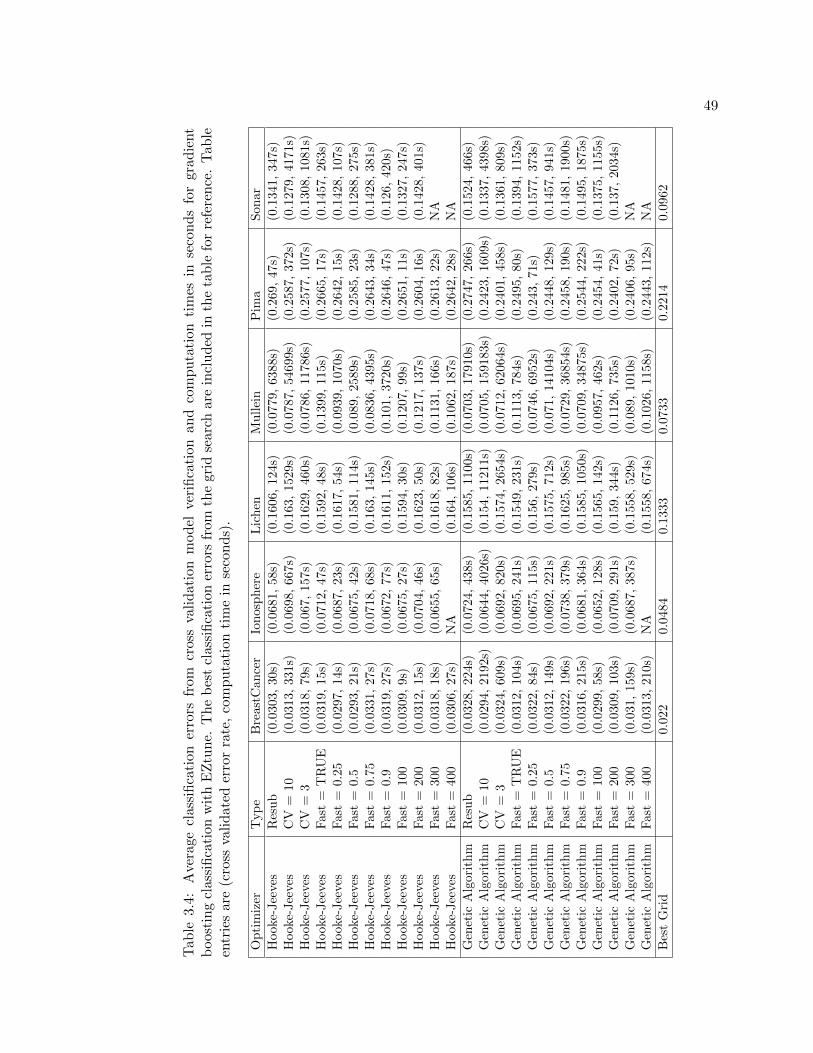
49
Tab
le3.
4:A
vera
gecl
assi
fica
tion
erro
rsfr
omcr
oss
vali
dat
ion
mod
elve
rifi
cati
onan
dco
mp
uta
tion
tim
esin
seco
nd
sfo
rgr
adie
nt
boos
ting
class
ifica
tion
wit
hE
Ztu
ne.
Th
eb
est
clas
sifi
cati
oner
rors
from
the
grid
sear
char
ein
clud
edin
the
tab
lefo
rre
fere
nce
.T
able
entr
ies
are
(cro
ssva
lid
ate
der
ror
rate
,co
mp
uta
tion
tim
ein
seco
nd
s).
Opti
miz
erT
yp
eB
reas
tCan
cer
Ionos
pher
eL
ichen
Mullei
nP
ima
Son
ar
Hook
e-Jee
ves
Res
ub
(0.0
303,
30s)
(0.0
681,
58s)
(0.1
606,
124s
)(0
.077
9,63
88s)
(0.2
69,
47s)
(0.1
341,
347s
)H
ook
e-Jee
ves
CV
=10
(0.0
313,
331s
)(0
.069
8,66
7s)
(0.1
63,
1529
s)(0
.078
7,54
699s
)(0
.258
7,37
2s)
(0.1
279,
4171
s)H
ook
e-Jee
ves
CV
=3
(0.0
318,
79s)
(0.0
67,
157s)
(0.1
629,
460s
)(0
.078
6,11
786s
)(0
.257
7,10
7s)
(0.1
308,
1081
s)H
ook
e-Jee
ves
Fast
=T
RU
E(0
.031
9,15
s)(0
.071
2,47
s)(0
.159
2,48
s)(0
.139
9,11
5s)
(0.2
665,
17s)
(0.1
457,
263s
)H
ook
e-Jee
ves
Fast
=0.
25
(0.0
297,
14s)
(0.0
687,
23s)
(0.1
617,
54s)
(0.0
939,
1070
s)(0
.264
2,15
s)(0
.142
8,
107s
)H
ook
e-Jee
ves
Fast
=0.
5(0
.029
3,21
s)(0
.067
5,42
s)(0
.158
1,11
4s)
(0.0
89,
2589
s)(0
.258
5,23
s)(0
.128
8,
275s
)H
ook
e-Jee
ves
Fast
=0.
75
(0.0
331,
27s)
(0.0
718,
68s)
(0.1
63,
145s
)(0
.083
6,43
95s)
(0.2
643,
34s)
(0.1
428,
381s
)H
ook
e-Jee
ves
Fast
=0.
9(0
.031
9,27
s)(0
.067
2,77
s)(0
.161
1,15
2s)
(0.1
01,
3720
s)(0
.264
6,47
s)(0
.126
,42
0s)
Hook
e-Jee
ves
Fast
=10
0(0
.030
9,9s
)(0
.067
5,27
s)(0
.159
4,30
s)(0
.120
7,99
s)(0
.265
1,11
s)(0
.132
7,
247s
)H
ook
e-Jee
ves
Fast
=20
0(0
.031
2,15
s)(0
.070
4,46
s)(0
.162
3,50
s)(0
.121
7,13
7s)
(0.2
604,
16s)
(0.1
428,
401s
)H
ook
e-Jee
ves
Fast
=30
0(0
.031
8,18
s)(0
.065
5,65
s)(0
.161
8,82
s)(0
.113
1,16
6s)
(0.2
613,
22s)
NA
Hook
e-Jee
ves
Fast
=40
0(0
.030
6,27
s)N
A(0
.164
,10
6s)
(0.1
062,
187s
)(0
.264
2,28
s)N
A
Gen
etic
Alg
ori
thm
Res
ub
(0.0
328,
224s
)(0
.072
4,43
8s)
(0.1
585,
1100
s)(0
.070
3,17
910s
)(0
.274
7,26
6s)
(0.1
524,
466s
)G
enet
icA
lgori
thm
CV
=10
(0.0
294,
2192
s)(0
.064
4,40
26s)
(0.1
54,
1121
1s)
(0.0
705,
1591
83s)
(0.2
423,
1609
s)(0
.133
7,
4398
s)G
enet
icA
lgori
thm
CV
=3
(0.0
324,
609s
)(0
.069
2,82
0s)
(0.1
574,
2654
s)(0
.071
2,62
064s
)(0
.240
1,45
8s)
(0.1
361,
809s
)G
enet
icA
lgori
thm
Fast
=T
RU
E(0
.031
2,10
4s)
(0.0
695,
241s
)(0
.154
9,23
1s)
(0.1
113,
784s
)(0
.249
5,80
s)(0
.139
4,
1152
s)G
enet
icA
lgori
thm
Fast
=0.
25
(0.0
322,
84s)
(0.0
675,
115s
)(0
.156
,27
9s)
(0.0
746,
6952
s)(0
.243
,71
s)(0
.157
7,
373s
)G
enet
icA
lgori
thm
Fast
=0.
5(0
.031
2,14
9s)
(0.0
692,
221s
)(0
.157
5,71
2s)
(0.0
71,
1410
4s)
(0.2
448,
129s
)(0
.145
7,
941s
)G
enet
icA
lgori
thm
Fast
=0.
75
(0.0
322,
196s
)(0
.073
8,37
9s)
(0.1
625,
985s
)(0
.072
9,36
854s
)(0
.245
8,19
0s)
(0.1
481,
1900
s)G
enet
icA
lgori
thm
Fast
=0.
9(0
.031
6,21
5s)
(0.0
681,
364s
)(0
.158
5,10
50s)
(0.0
709,
3487
5s)
(0.2
544,
222s
)(0
.149
5,
1875
s)G
enet
icA
lgori
thm
Fast
=10
0(0
.029
9,58
s)(0
.065
2,12
8s)
(0.1
565,
142s
)(0
.095
7,46
2s)
(0.2
454,
41s)
(0.1
375,
1155
s)G
enet
icA
lgori
thm
Fast
=20
0(0
.030
9,10
3s)
(0.0
709,
291s
)(0
.159
,34
4s)
(0.1
126,
735s
)(0
.240
2,72
s)(0
.137
,20
34s)
Gen
etic
Alg
ori
thm
Fast
=30
0(0
.031
,15
9s)
(0.0
687,
387s
)(0
.155
8,52
9s)
(0.0
89,
1010
s)(0
.240
6,95
s)N
AG
enet
icA
lgori
thm
Fast
=40
0(0
.031
3,21
0s)
NA
(0.1
558,
674s
)(0
.102
6,11
58s)
(0.2
443,
112s
)N
A
Bes
tG
rid
0.02
20.
0484
0.13
330.
0733
0.22
140.
096
2

50
Hooke−Jeeves
Genetic Algorithm
0.00
0.25
0.50
0.75
1.00
0.00
0.25
0.50
0.75
1.00
Sta
ndar
dize
d E
rror
Rat
eGradient Boosting Machine
BreastCancer
Ionosphere
Lichen
Mullein
Pima
Sonar
Hooke−Jeeves
Genetic Algorithm
Resub
CV = 1
0
CV = 3
Fast
= TRUE
Fast
= 0.
25
Fast
= 0.
5
Fast
= 0.
75
Fast
= 0.
9
Fast
= 10
0
Fast
= 20
0
Fast
= 30
0
Fast
= 40
0
0.00
0.25
0.50
0.75
1.00
0.00
0.25
0.50
0.75
1.00
Sta
ndar
dize
d T
ime
Fig. 3.4: Standardized classification error rates and computation times for gradient boostingclassification. The best error rates and computation times for each dataset have a value of0 and the worst have a value of 1.

51
Tab
le3.5
:A
vera
ge
clas
sifi
cati
oner
rors
from
cros
sva
lid
atio
nm
od
elve
rifi
cati
onan
dco
mp
uta
tion
tim
esin
seco
nd
sfo
rad
aboos
tw
ith
EZ
tun
e.T
he
bes
tcl
assi
fica
tion
erro
rsfr
omth
egr
idse
arch
are
incl
ud
edin
the
tab
lefo
rre
fere
nce
.T
able
entr
ies
are
(cro
ssva
lid
ated
erro
rra
te,
com
pu
tati
onti
me
inse
con
ds)
.
Opti
miz
erT
yp
eB
reas
tCan
cer
Ionos
pher
eL
ichen
Mullei
nP
ima
Son
ar
Hook
e-Jee
ves
Res
ub
(0.0
347,
131s
)(0
.073
8,20
7s)
(0.1
689,
381s
)(0
.125
4,12
601s
)(0
.278
6,12
16s)
(0.1
668
,234
s)H
ook
e-Jee
ves
CV
=10
(0.0
351,
1568
s)(0
.081
2,21
45s)
(0.1
615,
3472
s)(0
.126
5,12
3910
s)(0
.245
2,87
02s)
(0.1
659
,309
9s)
Hook
e-Jee
ves
CV
=3
(0.0
344,
455s
)(0
.078
1,66
2s)
(0.1
615,
1086
s)(0
.125
5,27
970s
)(0
.240
9,25
96s)
(0.1
553
,851
s)H
ook
e-Jee
ves
Fas
t=
TR
UE
(0.0
357,
114s
)(0
.075
5,22
1s)
(0.1
65,
299s
)(0
.179
5,52
8s)
(0.2
518,
709s
)(0
.1663
,322
s)H
ook
e-Jee
ves
Fas
t=
0.25
(0.0
34,
114s
)(0
.078
9,21
0s)
(0.1
708,
298s
)(0
.129
8,29
64s)
(0.2
49,
672s)
(0.1
582
,265
s)H
ook
e-Jee
ves
Fas
t=
0.5
(0.0
36,
148s
)(0
.076
4,19
8s)
(0.1
638,
322s
)(0
.127
2,62
86s)
(0.2
574,
778s
)(0
.1524
,315
s)H
ook
e-Jee
ves
Fas
t=
0.75
(0.0
334,
163s
)(0
.078
9,21
8s)
(0.1
599,
386s
)(0
.129
2,78
31s)
(0.2
479,
909s
)(0
.1562
,302
s)H
ook
e-Jee
ves
Fas
t=
0.9
(0.0
354,
145s
)(0
.077
2,24
5s)
(0.1
658,
370s
)(0
.132
7,90
46s)
(0.2
496,
940s
)(0
.1471
,312
s)H
ook
e-Jee
ves
Fas
t=
100
(0.0
366,
108s
)(0
.077
8,17
4s)
(0.1
667,
227s
)(0
.187
4,41
2s)
(0.2
543,
595s
)(0
.1591
,316
s)H
ook
e-Jee
ves
Fas
t=
200
(0.0
34,
124s
)(0
.076
6,23
9s)
(0.1
682,
220s
)(0
.186
4,44
5s)
(0.2
491,
767s
)(0
.1639
,228
s)H
ook
e-Jee
ves
Fas
t=
300
(0.0
351,
128s
)(0
.079
5,23
2s)
(0.1
667,
310s
)(0
.194
2,42
7s)
(0.2
418,
705s
)N
AH
ook
e-Jee
ves
Fas
t=
400
(0.0
348,
150s
)N
A(0
.168
7,29
7s)
(0.1
802,
523s
)(0
.247
,70
3s)
NA
Gen
etic
Alg
ori
thm
Res
ub
(0.0
306,
523s
)(0
.071
8,84
7s)
(0.1
582,
1999
s)(0
.113
7,51
756s
)(0
.276
,41
91s
)(0
.1404
,107
0s)
Gen
etic
Alg
ori
thm
CV
=10
(0.0
327,
5165
s)(0
.070
4,12
083s
)(0
.163
5,22
474s
)(0
.128
2,22
4020
s)N
A(0
.1341
,146
81s)
Gen
etic
Alg
ori
thm
CV
=3
(0.0
318,
1772
s)(0
.068
7,29
17s)
(0.1
573,
5970
s)(0
.120
2,77
899s
)(0
.260
7,12
742s
)(0
.1365
,412
8s)
Gen
etic
Alg
ori
thm
Fas
t=
TR
UE
(0.0
31,
568s
)(0
.072
4,79
3s)
(0.1
619,
1228
s)(0
.141
2,18
37s)
(0.2
698,
3064
s)(0
.1351
,135
8s)
Gen
etic
Alg
ori
thm
Fas
t=
0.25
(0.0
328,
528s
)(0
.069
8,73
8s)
(0.1
587,
1305
s)(0
.126
5,11
429s
)(0
.264
2,35
88s)
(0.1
413
,112
0s)
Gen
etic
Alg
ori
thm
Fas
t=
0.5
(0.0
321,
641s
)(0
.072
4,84
8s)
(0.1
543,
1395
s)(0
.128
1,21
992s
)(0
.261
8,35
08s)
(0.1
457
,121
0s)
Gen
etic
Alg
ori
thm
Fas
t=
0.75
(0.0
3,67
6s)
(0.0
709,
1070
s)(0
.161
1,17
70s)
(0.1
25,
3571
9s)
(0.2
674,
4699
s)(0
.1317
,133
2s)
Gen
etic
Alg
ori
thm
Fas
t=
0.9
(0.0
316,
473s
)(0
.070
9,79
4s)
(0.1
571,
2247
s)(0
.127
7,47
479s
)(0
.266
1,51
61s)
(0.1
308
,128
3s)
Gen
etic
Alg
ori
thm
Fas
t=
100
(0.0
335,
428s
)(0
.072
9,94
4s)
(0.1
608,
933s
)(0
.138
3,13
37s)
(0.2
745,
2580
s)(0
.1418
,109
9s)
Gen
etic
Alg
ori
thm
Fas
t=
200
(0.0
309,
466s
)(0
.072
1,82
5s)
(0.1
57,
1165
s)(0
.135
9,17
29s)
(0.2
682,
3134
s)(0
.1413
,113
7s)
Gen
etic
Alg
ori
thm
Fas
t=
300
(0.0
313,
821s
)(0
.074
6,85
9s)
(0.1
568,
1502
s)(0
.127
1,24
33s)
(0.2
755,
3895
s)N
AG
enet
icA
lgori
thm
Fas
t=
400
(0.0
324,
807s
)N
A(0
.159
9,15
76s)
(0.1
294,
2619
s)(0
.266
9,43
92s)
NA
Bes
tG
rid
0.01
90.
0484
0.12
50.
0814
0.21
090.
0865
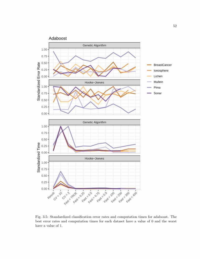
52
Hooke−Jeeves
Genetic Algorithm
0.00
0.25
0.50
0.75
1.00
0.00
0.25
0.50
0.75
1.00
Sta
ndar
dize
d E
rror
Rat
eAdaboost
BreastCancer
Ionosphere
Lichen
Mullein
Pima
Sonar
Hooke−Jeeves
Genetic Algorithm
Resub
CV = 1
0
CV = 3
Fast
= TRUE
Fast
= 0.
25
Fast
= 0.
5
Fast
= 0.
75
Fast
= 0.
9
Fast
= 10
0
Fast
= 20
0
Fast
= 30
0
Fast
= 40
0
0.00
0.25
0.50
0.75
1.00
0.00
0.25
0.50
0.75
1.00
Sta
ndar
dize
d T
ime
Fig. 3.5: Standardized classification error rates and computation times for adaboost. Thebest error rates and computation times for each dataset have a value of 0 and the worsthave a value of 1.

53
and adaboost. The package includes a function that can quickly compute cross validated
error measure so that the user can use faster methods to find a model and then obtain a
more accurate error measure.
Package performance tests show that optimizing on resubstitution error does not prod-
uct good results, particularly for regression models. It is also not particularly fast, so this
method is not recommended. The best error measures are obtained when 10-fold cross
validation is done, but it also has the slowest computation times. The fast options in the
function typically produce models with lower error measures with fast computation times.
The larger datasets get much better error measures when at least 50% of the data are used
for the training dataset. Models computed for small datasets are not stable and that should
be considered when using EZtune. Adaboost does not perform as well as SVM and GBM
and it had the longest computation times. The overall best performing options seem to be
SVM and GBM with 10-fold cross validation if the time can be spared, or a fast option that
uses at least 50% of the data to train the model. The fast default option is very fast and
performs well for moderately sized datasets.
CHAPTER 4
THREE-PHASE FILTERING METHOD FOR GENOME-WIDE ASSOCIATION
STUDIES
4.1 Introduction
GWAS has been done since the early 2000s and continues to be an active field of
research. Many methods for GWAS continue to be developed to address the many diffi-
culties that arise with analyses of ultra-high dimensional datasets with complex structure.
It is difficult to identify SNPs that are weakly associated with a phenotype, but identi-
fication of these SNPs is important for understanding how genetics affect physical traits.
Another complication is LD, which can cause SNPs to be erroneously identified as asso-
ciated with a phenotype when they are, in fact, only associated with a nearby SNP that
is associated [Chen et al., 2011]. Many of the GWAS methods rely on statistical methods
that produce a p-value for each SNP. This escalates the multiple statistical testing issue
to a level that correction measures were never intended to address [Wellcome Trust Case
Control Consortium, 2007].
This chapter explores some of these issues using several common GWAS methods and
using a few that have not been previously used in a GWAS setting, but have been used
extensively for feature selection. The method is comprised of three phases. The first
phase consists of a simple filter that uses distance correlation [Szekely et al., 2007], linear
regression, or logistic regression to remove noise from the dataset [Zeng et al., 2015]. The
SNPs that are retained are further trimmed using either a LASSO or elastic net model
[Waldmann et al., 2013]. This further removes noise while allowing all of the SNPs that
pass through the first filter to assess as a group rather than in isolation. The last phase of
the method uses either random forests [Breiman, 2001] or CART [Breiman et al., 1984] to
identify SNPs that are most strongly associated with the phenotype.

55
This method was developed by reading GWAS papers that use distance correlation
[Carlsen et al., 2016], linear regression, and logistic regression to identify SNPs associated
with the phenotype. These methods are rarely used in isolation because they contain many
false-positive values due to LD. However, they are a useful tool in eliminating noise [Zeng
et al., 2015]. LASSO and other penalized regression methods have gained popularity as a
method for finding a subset of SNPs that should be further evaluated for association with the
phenotype [Wu et al., 2009]. LASSO has a low false positive rate, but it also has a high false
negative rate. Elastic net has been examined as an alternative to avoid the large number
of false negatives, but it has a much higher false positive rate than LASSO [Waldmann
et al., 2013]. As the value of α decreases for elastic net, the number of false positives
increases, but the number of false negatives decreases. Both LASSO and elastic net require
additional evaluation for SNPs with non-zero coefficients. Methods involving linear and
logistic regression and the FDR have been proposed [Wu et al., 2009], but there is much
exploration that is still needed with this phase. Tuning λ and α is also an area that needs
further exploration [Waldmann et al., 2013]. We replicated the logistic regression method
for final SNP selection on several datasets and found that it appeared to work well in some
situations, but not in others. It is also unclear what a good FDR cutoff value is for final
SNP selection. Because random forests and CART can be used for more refined feature
selection and do not rely on p-values, we explore the use of these tools in lieu of logistic
and linear regression for the final phase of our method.
The exploration done for this chapter uses simulated data with low heritability. Most
of the papers we read on GWAS that used simulated data did not disclose the level of
heritability in the simulated data. We decided to conduct our exploration of these methods
using only data with heritability of 0.1, 0.3, and 0.8 because these levels are indicative of
what is see in nature and what is expected for a GWAS in a medical setting. This analysis
shows that heritability has a strong impact on the efficacy of all of these methods.
4.2 Method
Data were simulated using the genomes of a fruit fly (Rhagoletis pomonella) [Egan

56
et al., 2015], a stick insect (Timema cristinae) [Comeault et al., 2015], and an NMRI
mouse population [Zhang et al., 2012]. Different options within the GWAS method were
tested to determine performance using the following methodology.
4.2.1 Data Simulation
Data were simulated using genomes obtained from three different animals. A descrip-
tion of the data is in Table 4.1. SNPs were randomly selected to be functional SNPs, that
is, SNPs that have a direct outcome on the phenotype, and then phenotypes were gener-
ated such that they only rely on the functional SNPs. Because natural systems are noisy,
random noise was added to the computed phenotype to make the data more realistic. The
amount of noise that is introduced is determined by the desired amount of heritability.
The heritability is a measure of how much the genotype influences the phenotype [National
Institutes of Health United States Library of Medicine, 2019]. It is equivalent to R2 in
statistics. This method produces simulated data that retains all of the complexity of the
genotype while allowing for control of data characteristics that impact the relationship be-
tween the genotype and phenotype. The algorithm for generating the simulated data is
shown in Algorithm 1.
Table 4.1: List of datasets used for data simulation.
Dataset Type of Animal Number of Observations Number of SNPs
Rhagoletis Pomonella Fruit Fly 149 33,723Timema Cristinae Stick Insect 592 246,258NMRI Mice Mouse 288 44,428
Phenotypes were created using 5, 10, and 50 SNPs and using heritabilities of 0.1, 0.3,
and 0.8 for each of the datasets. These levels of heritability were selected because they mimic
different natural scenarios. Heritabilities of 0.1 and 0.3 are often seen in ecological settings,
but in medical genetics heritabilities of 0.8 or larger are often seen. Six phenotypes were
simulated for each dataset using each combination of these settings. Three of the phenotypes
were left as continuous and three were changed to binary responses. This resulted in a total

57
Algorithm 1: Generating simulated data for genome-wide association studies.
1 Determine how many SNPs will be functional SNPs (N). That is, how many SNPswill have a direct impact on the phenotype. Randomly select N SNPs from all ofthe SNPs in the genotype.
2 Generate N normal random variables with a mean of 0 and standard deviation of1. These values form the vector of effects.
3 Use the random normal variables as coefficients in a linear model and compute aphenotype for each observation using the equation:phenotype = effect× (functional SNPs).
4 Compute the variation for the noise that will be added to the phenotype using thedesired heritability with:V ar(phenotype noise) = V ar(phenotype)× 1−heritability
heritability
5 Create random noise for the phenotype by computing random normal variableswith µ = 0 and σ2 = V ar(phenotype noise).
6 Add the noise to the phenotype.7 If a binary phenotype is desired, change all of the phenotype values less than the
median to 0 and the values greater than or equal to the median to 1.
of thirty-six simulated phenotypes for each of the three genotypes.
4.2.2 Initial Filtering
The first step in the method is to remove the majority of the SNPs from the remainder
of the analysis using a simple filter. Filters are based on distance correlation and linear or
logistic regression, depending on the type of response variable. Filtering using single SNP
analysis and using neighborhoods of SNPs were tested.
Distance correlation is a measure of dependence introduced in 2007 that has gained
popularity in GWAS. It is similar to the product-moment correlation, but it is only 0
if the random vectors are independent. The distance correlation is based on Euclidean
distances between sample elements rather than sample moments. It can be used both on
continuous and binary variables. Distance correlation measures were obtained for each SNP
by comparing a single SNP with the phenotype and also by comparing neighborhoods of 10
SNPs at a time with the phenotype. Distance correlations were computed using the energy
package [Rizzo and Szekely, 2018].
Linear and logistic regression filters were treated in the same manner and will be

58
referred to as the regression models to avoid redundancy. Regression models were computed
both by using a single SNP as a predictor and by using a neighborhood of 10 SNPs around
a SNP as the predictors. If the predictor was a single SNP, the p-value on the coefficient
was recorded as the filter value for that SNP. If the predictors included the SNP and the
neighborhood around the SNP, the p-value for the likelihood ratio test was used as the filter
value for that SNP. Both the raw p-values and the FDR were examined to determine which
method produced better final results after all stages of the GWAS method.
Once the filter values are computed, several methods can be used to determine which
SNPs to keep for the next phase of analysis. The distance correlations or p-values can
be plotted using a Manhattan plot and an appropriate threshold can be visually selected.
Another method is to select the number of SNPs that will pass through the filter and retain
that number of SNPs. The latter method was used to ensure that the method could be
tested in the second phase with a dataset that had more SNPs than observations and with
a dataset that had fewer SNPs than observations. This was done to see how the n<p
issue affected the LASSO and elastic net phase of the GWAS method. Seventy-five and 175
SNPs retained from the R. pomonella data, 300 and 700 were retained from the T. chrisinae
data, and 150 and 350 from the mouse data. Slightly more than this were retained from
the data that used a window of ten SNPs around the target SNP because if a a SNP has a
distance correlation or p-value that passes through the filter, the entire set of eleven SNPs
was retained.
An advantage of using distance correlation and regression in this manner is that the
data can be partitioned and calculations can be done in sections. This can speed up com-
putation time by allowing for parallelization with a cluster computing system or allowing
the user to perform computations over several different R sessions. Large genotypes are
computationally accessible using a personal computer. Once the initial filtering is done, the
LASSO, elastic net, random forest, and CART calculations are fast because the data are
manageable in size.

59
4.2.3 LASSO and Elastic Net for Further Refinement
LASSO and elastic net models were computed using the data that passed through the
first phase of filtering. Computations were done using the glmnet package in R. Cross
validation was used to select a value for λ on the LASSO model. This value of λ was used
for the LASSO and all of the elastic net models computed for a dataset. Multiple values
of α were used to determine how parameter selection affected final SNP selection and the
ability of this second phase to detect SNPs with even a small effect. Values were α = 0,
0.005, 0.01, 0.1, 0.25, 0.5, 0.75, 0.9, 1.0, where α = 0 will allow all of the SNPs to pass onto
the third phase of the method and allow for assessment of the necessity of this phase. SNPs
that have non-zero coefficients are passed onto the third phase of the GWAS method.
4.2.4 Random Forests and Classification and Regression Trees for Final SNP
Selection
The final stage of this GWAS method uses the SNPs that have non-zero coefficients
to compute a CART and a random forest. The trees created by CART were pruned using
the 1-se rule. All SNPs where the pruned tree splits are considered SNPs with a strong
association with the phenotype. This selection criteria is automatic and does not require
user subjectivity.
Random forests compute an importance measure for each of the predictors. This mea-
sure was examined graphically to determine which SNPs are important. This method
involves subjectivity in that the variable importance plot is visually inspected and natural
changes in the importance measures are used to determine a threshold for the SNPs that
are most associated with each phenotype.
4.2.5 Final Assessment of Results
It was anticipated that the final SNP selection part of this method is too restrictive to
identify SNPs that are associated with the phenotype that have a small effect. The LASSO
and elastic net piece was designed to identify SNPs that are associated, but have a small
effect. The random forests and CART portion of the method are used to identify the SNPs

60
that have the strongest association with the phenotype. Both pieces were examined to see
how much noise is picked up in the elastic net phase of testing and how sensitive the final
phase is.
It is known that when data are genotyped a SNP that is primarily associated with the
phenotype may not be sequenced, but its neighbors may be. The purpose of a GWAS is
not to identify the causal SNP, but to identify a region where there is a likely causal SNP.
This means that if the SNP that is most strongly associated with the trait is not sequenced
the area may still be identified as important because of the LD in the region. Because of
this, it is not essential that a specific SNP is identified, but rather it is important that a
SNP nearby is identified. Because of this, results not only consider identification of a SNP
that was chosen to be a functional SNP during simulation to be a true-positive, but if a
SNP nearby is chosen it is also considered a successful find.
The results were assessed graphically to see how closely the SNPs selected at various
stages of the method lined up with the associated SNPs. The graphs display the associated
SNPs along with their effect, the results of the initial filter, the SNPs that pass through the
different elastic net model, the SNPs selected by trees, and the importance of each of the
SNPs that pass through elastic net as determined by random forest. Figure 4.1 shows an
example plot. The x-axis represents the position of each SNP along the genome. The red
lines on the plot show the associated SNPS with the height of the line scaled to represent
the effect size of each SNP. Taller lines represent SNPs with a larger effect. The gray dots
on the plot show the results of the initial filter with the y-axis. If the filter was a distance
correlation the raw values are displayed. If the filter was a regression model, the y-axis is
− log10(p). The dots underneath the filter graph represent the results of the rest of the SNP
selection method. The purple points show the SNPs that had non-zero coefficients in the
elastic net model. The blue points are the SNPs that were selected by CART. The green
points show all of the SNPs that had non-zero coefficients with the elastic net model, but the
size represents the importance of each SNPs with larger importance measures represented
by circles with larger radii.

61
Fig. 4.1: Example plot for assessing the performance of the GWAS method with the mousedata. The radius of the green circles represents the importance as determined by randomforests. The blue circles represent the SNPs that trees found to be important and purplecircles represent the SNPs with non-zero coefficients in the elastic net model. The radiusof the blue and purple circles does not represent anything. The red lines show the positionof the functional SNPs.

62
4.3 Results
The graphs proved insightful in assessing what was happening across all phases of the
method. It was clear that the ability of the initial filter to find the associated SNPs was
critical to finding the SNPs through the other stages of the method. If the initial filter could
not see that there was an associated SNP, elastic net, CART, and random forests could not
identify the SNP either. The following provides a summary of what was observed in the
graphs.
4.3.1 Heritability
Heritability proved to be the most important factor in how well the method performed.
When the heritability was very low, none of the filters were able to find the associated SNPs.
When heritability was high, filters were able to find many of the associated SNPs. When the
heritability was low (0.1 or 0.3) the filter plots often looked as if they were finding signals,
but when compared to the associated SNPs it was noise. Occasionally, the filters were able
to find SNPs with a strong signal, but they often missed even the most strongly associated
SNPs when the heritability was low. A heritability of 0.3 produced better results and the
filters were able to find some of strongly associated SNPs. However, the success rate with
this was unsatisfactorily low. When the heritability was increased to 0.8, the filters had
much more success at detecting the target SNPs. Variables selected by elastic net typically
covered the regions with associated SNPs and tree and random forest variable selection
found many of the SNPs. Figures 4.2 - 4.11 show a clear pattern on how heritability affects
the ability to identify functional SNPs.
4.3.2 Initial Filter
The plots for the initial filters differed in appearance based on the type of filter used.
The filters using the raw p-values for a linear or logistic regression model appear to have
stronger signals, as seen in Figure 4.8, while the regression models using FDR have few
strong signals as in Figure 4.9. Figure 4.10 shows the distance correlation has weaker ap-
pearing signals than the raw p-values as well. However, comparison with the truly associated

63
SNPs shows that the supposed strong signals with the raw p-values are often false-positives
and that many of even the most strongly associated SNPs are not observed with the filter
when heritability was low. When heritability was high, the filters were able to capture the
SNPs that were associated along with many that were not associated. The FDR p-values
frequently do not show a signal, but they find associated SNPs as often as the raw p-values.
Distance correlation performs similarly well to the regression filters. Although all of the
filters choose different subsets of potentially significant SNPs, none of the filters seem to
outperform the others.
The number of points that were allowed through did not seem to have an affect on
the performance of the method in future phases for low heritability. When heritability was
0.8 more SNPs were selected by elastic net for the larger filter size, but it rarely made an
impact on the SNPs selected by trees or random forests.
Testing a neighborhood around each SNP did seem to matter slightly for low heritabil-
ity. When we tested SNPs in groups of 10, the performance of the method was worse. For
a higher heritability it did not matter if a single SNP or neighborhood of SNPs was used.
4.3.3 Elastic Net
It was hoped that the elastic net would be able to detect the underlying architecture
of the associated SNPs, even with low heritability. Most of the time associated SNPs were
in regions that had non-zero coefficients. However, the SNPs identified by elastic net were
frequent in regions that were not near associated SNPs and sometimes elastic net did not
represent regions with strongly associated SNPs as seen in Figure 4.2. The selection of α
is difficult to assess as well. When α is close to 0, so many SNPs are often selected it is
not particularly helpful in assessing architecture. When α is close to 1, far fewer SNPs are
selected and the regions of associated SNPs are often identified, but areas with associated
SNPs are also more likely to get missed. Figure 4.2 shows that sometimes elastic net fails
to find many associated SNPs even with low levels of α when the heritability is small.
When heritability was 0.8, elastic net typically selected SNPs from regions that included
the associated SNPs. This was not always the case, but for most of the tests run, elastic

64
Fig. 4.2: NMRI mouse data with heritability of 0.1 demonstrating inability of filter to findtruly associated SNPs.

65
Fig. 4.3: NMRI mouse data with heritability of 0.3 demonstrating inability of filter to findtruly associated SNPs.

66
Fig. 4.4: NMRI mouse data with heritability of 0.8 demonstrating improvement in methodwith stronger heritability.

67
Fig. 4.5: T. cristinae data with heritability of 0.1 demonstrating inability of filter to findtruly associated SNPs.

68
Fig. 4.6: T. cristinae data with heritability of 0.3 demonstrating inability of filter to findtruly associated SNPs.

69
Fig. 4.7: T. cristinae data with heritability of 0.8 demonstrating improvement in methodwith stronger heritability.

70
Fig. 4.8: R. pomonella data with heritability of 0.3 and with the linear regression filterusing the FDR p-values transformed using − log10 P . This plot demonstrates inability offilter to find truly associated SNPs with such low heritability and the difference in the filterplot between FDR p-values and raw p-values.

71
Fig. 4.9: R. pomonella data with heritability of 0.3 and with the linear regression filter withthe raw p-values transformed using − log10 P . This plot demonstrates inability of filter tofind truly associated SNPs with such low heritability and the difference in the filter plotbetween distance correlation, the FDR p-values, and raw p-values.

72
Fig. 4.10: R. pomonella data with heritability of 0.3 and with the distance correlationfilter. This plot demonstrates inability of filter to find truly associated SNPs with suchlow heritability and the difference in the filter plot between distance correlation, the FDRp-values, and raw p-values.

73
Fig. 4.11: R. pomonella data with heritability of 0.8 demonstrating improvement in methodwith stronger heritability.

74
net covered the desired regions as in Figure 4.7. When α was small, the number of SNPs
with non-zero coefficients was often too large to be particularly helpful. When α was large,
the number of SNPs was small enough to help narrow down the genome. Elastic net results
often missed some of the exact associated SNPs, but it would show the region as being
associated.
4.3.4 Random Forests and CART
Random forests and CART had mixed results. CART often identified different SNP
regions as significant than random forests. There were many false positives and false nega-
tives with both methods. If the initial filter did not clearly identify a region as associated
with the phenotype, CART and random forests were not able to find those locations either.
Figures 4.2 - 4.11 demonstrate these qualities of CART and random forests.
Some patterns were detected in the tests where heritability was 0.8. Random forests
did not find as many SNPs as CART, but it rarely had a false positive. Essentially, it
was not able to find associated SNPs as well, but when it found one, it was most likely
associated. CART found more of the associated SNPs that random forests, but had quite a
few false-positives. A combination of CART and random forests was often able to find the
SNPs most strongly associated with the phenotype, but not always. This was particularly
true for the mouse data.
4.3.5 Datasets
The methods performed differently for the different datasets. Although none of them
performed particularly well, all of the methods performed better on the mouse data than on
the R. pomonella data. The filters were better able to find signals in the associated SNPs
even for the lowest level of heritability. However, there are still many false positives and
false negatives with the mouse data and the T cristenae data.
4.4 Conclusions
Evaluation of linear models, distance correlation, elastic net, CART, and random forests

75
show that when heritability is low, these methods are not able to identify associated SNPs
well. When heritability is high, they can find many of the most strongly associated SNPs,
but there are still many false negatives. Linear models and distance correlation were used
as initial filters to remove the majority of the noise from the data, but all of the filters
had difficulty finding the regions where the associated SNPs were located unless heritability
is strong. The inability of the initial filter to identify the locations of associated SNPs
percolated down through the rest of the methods that were tested. Elastic net and LASSO
are often used in GWAS to find associated SNPs, but when heritability is low, elastic net
struggles to identify important regions and misses many of the areas of highest association.
Random forests and CART are also unable to identify areas of association when the filters
fail to find them in that situation. When heritability is strong, CART and random forest
often find the most strongly associated SNPs, but they sometimes miss a few and typically
miss SNPs that have a weaker association. Random forests usually selects fewer SNPs than
CART, but the are more likely to be true positives.
This exploration shows that heritability must be carefully considered when evaluating
methods for GWAS using simulated data. It is not sufficient to simulate data with a
known architecture to evaluate a method. Heritability should be assessed from real datasets
to understand the level that can be expected in the type of problem being studied. If
heritability is low, as it often is, methods should be carefully selected to ensure they can
detect associated SNPs in that situation. If a new method is developed, it should be tested
to evaluate the limitations of performance with different levels of heritability so that its
limitations are well understood.

CHAPTER 5
FUTURE WORK AND CONCLUSIONS
In Chapter 2, we explored tuning parameters for SVMs, GBMs, and adaboost. We were
able to find tuning parameter spaces for each of the methods and find a fast optimization
algorithm for tuning a good model. Other statistical learning models, such as elastic net,
require tuning and similar evaluation for the behavior of α and λ would be beneficial.
Random forests typically performs well without additional tuning, but for datasets with
many features, the default parameter values do not perform well. We used R to explore the
tuning parameters, but Python is a powerful tool for machine learning and the functions
available in sci-kit learn [Pedregosa et al., 2011] may behave differently than those in R.
Replication of the analysis presented in this dissertation in Python could add insight into
the behavior of tuning parameters and may provide additional options for finding an optimal
model.
In Chapter 3 we presented the R package EZtune, which was written using the research
presented in Chapter 2. Further work can be done by providing a tool for tuning elastic
net and for including options for tuning random forests with large datasets. A multi-class
model tuning feature is also planned for the future. The current options in R for computing
multi-class models for SVM, GBM, and adaboost are computationally far more expensive
than those for binary classification or regression. Optimization algorithms failed to tune
the model with reasonable computation time. Python does not have an automatic tuning
tool similar to EZtune so we plan to do a Python implementation as well. Python has
some tools that may allow for expansion of capabilities beyond what can be done in R at
this time because of faster computation times. In particular, multi-class model tuning and
faster adaboost implementation may be more feasible in Python than it is in R.
Chapter 4 explores the behavior of some common, and not so common, GWAS tools for
different sizes of heritability. We found that the methods that were tested did not perform

77
well with low heritability. Further work can be done by testing other commonly used
GWAS methods for a range of heritability values to determine how the different methods
perform with different physical traits. Our results show that when heritability is low it can
appear that there are strong signals where there is, in fact, no association at all. Careful
data simulation is needed to ensure methods are fully evaluated. In situations where we
are looking for SNPs that are associated with a specific disease, the heritability can be
estimated from real data and then simulated data can be created that more closely mimics
the physical characteristics of the data.

78
APPENDICES

79
APPENDIX A
EZtune Vignette
A.1 Introduction to EZtune
EZtune is an R package that can automatically tune support vector machines (SVMs),
gradient boosting machines (GBMs), and adaboost. The idea for the package came from
frustration with trying to tune supervised learning models and finding that available tools
are slow and difficult to use, have limited capability, or are not reliably maintained. EZtune
was developed to be easy to use off the shelf while providing the user with well tuned
models within a reasonable computation time. The primary function in EZtune searches
through the hyperparameter space for a model type using either a Hooke-Jeeves or genetic
algorithm. Models with a binary or continuous response can be tuned.
EZtune was developed using research that explored effective hyperparameter spaces
for SVM, GBM, and adaboost for data with a continuous response variable or with a
binary response variable. Many optimization algorithms were tested to identify ones that
were able to find an optimal model with reasonable computation time. The Hooke-Jeeves
optimization algorithm out-performed all of the other algorithms in terms of model accuracy
and computation time. A genetic algorithm was sometimes able to find a better model than
the Hooke-Jeeves optimizatation algorithm, but the computation time is significantly longer.
Thus, the genetic algorithm is included as an option, but it is not the default.
The package includes two functions and four datasets. The functions are eztune and
eztune cv. The datasets are lichen, lichenTest, mullein, and mulleinTest.
A.2 Functions: eztune and eztune cv
The eztune function is used to find an optimal model given the data. eztune cv provides
a cross validated accuracy or MSE for the model.

80
eztune
The eztune function is the primary function in the EZtune package. The only required
arguments are the predictors and the response variable. The function is built on existing R
packages that are well maintained and well programmed to ensure that eztune performance
is reliable. SVM models are computed using the e1071 package, GBMs with the gbm
package, and adaboost with the ada package. The models produced by eztune are objects
from each of these packages so all of the peripheral functions for these packages can be used
on models returned by eztune. A summary of each of these packages and why they were
chosen follows.
Support vector machines using the e1071 package
The e1071 package was written by and is maintained by David Meyer. The package
was built using the LIBSVM platform, which is written in C++ and is considered one
of the best open source libraries for SVMs. e1071 has been around for many years and
has continuously been updated during that time frame. It has all of the features needed
to perform the tasks needed by eztune and includes other features that allow expansion
of eztune in future versions, such as selection of kernels other than the radial kernel and
multi-class modeling.
Gradient boosting machines using the gbm package
The gbm package was written by Greg Ridgeway gbm and has been maintained and
updated for many years. It performs GBM by using the framework of an adaboost model
with an exponential loss function, but uses Friedman’s gradient descent algorithm to op-
timize the trees rather than the algorithm originally proposed in adaboost. This package
was selected because it had all of the features needed for eztune and included the ability to
compute a multi-class model for future EZtune versions.
Adaboost implementation with the ada package
In contrast to SVMs and GBMs, there are several standard packages in R that can be

81
used to fit adaboost models. The most established and well known package is ada. Other
packages that are often used are fastAdaboost and adabag. fastAdaboost is a new package
with a fast implementation of adaboost that is quickly gaining popularity. However, it
is still being developed and does not have all of the functionality needed for eztune. It
may be considered as a platform for later versions of eztune as fastAdaboost gains more
functionality because adaboost is currently the slowest model to tune. The package adabag
provides an implementation of adaboost that allows for bagging to be incorporated. This
feature is useful, but it does not allow for independent tuning of shrinkage or tree depth.
Because these parameters are important tuning parameters, adabag was not considered.
The ada package has been maintained and updated consistently for many years and has the
capability to tune the number of trees, tree depth, and shrinkage independently. Thus, ada
was chosen as the primary adaboost package for eztune.
Implementation of eztune
The eztune function was designed to be easy to use. It can be used when only data
are provided, but arguments can be changed for user flexibility. The default settings were
chosen to provide fast implementation of the function with good error rates. The syntax is:
eztune(x, y, method = "svm", optimizer = "hjn", fast = TRUE, cross = NULL)
The arguments are:
• x: matrix or data frame of dependent variables
• y: numeric vector of responses
• method: ”svm” for SVMs, ”ada” for adaboost, and ”gbm” for GBMs
• optimizer: ”hjn” for Hooke-Jeeves algorithm or ”ga” for genetic algorithm
• fast: Indicates if the function should use a subset of the observations when optimizing
to speed up calculation time. Options include TRUE, a number between 0 and 1, and
a positive integer. A value of TRUE will use the smaller of 50% of the data or 200

82
observations for model fitting. A number between 0 and 1 specifies the proportion
of data that will be used to fit the model. A positive integer specifies the number of
observations that will be used to fit the model. A model is computed using a random
selection of data and the remaining data are used to validate model performance.
Validation error rate or MSE is used as the optimization measure.
• cross: If an integer k<1 is specified, k-fold cross validation is used to fit the model.
This parameter is ignored unless fast = FALSE.
The function determines if a response is binary or continuous and then performs the
appropriate grid search based on the function arguments. Testing showed that the SVM
model is faster to tune than GBMs and adaboost, with adaboost being substantially slower
than either of the other models. Tuning is also very slow as datasets get large. The mullein
and lichen datasets included this package tune very slowly because of their size. Testing
the package on these datasets indicated that the fast options should be set as the default.
If a user wants a more accurate model and is willing to wait for it, they can select cross
validation or fit with a larger subset of the data.
The Hooke-Jeeves optimization algorithm was chosen as the default optimization tool
because it is fast and it outperformed all of the other algorithms tested. It did not always
produce the best model out of the algorithms, but it was the only algorithm that was always
among the best performers. The only other algorithm that consistently produced models
with error measures as low, or lower, than those found by the Hooke-Jeeves algorithm were
those found by the genetic algorithm. The genetic algorithm was able to find a much better
model than Hooke-Jeeves in some situations, so it is included in the package. However,
computation time for the genetic algorithm is very slow, particularly for large datasets. If
a user is in need of a more accurate model and can wait for a longer computation time,
the genetic algorithm is worth trying. However, eztune will typically produce a very good
model using the Hooke-Jeeves option with a much faster computation time. The function
hjn from the optimx package optimx is used to implement the Hooke-Jeeves algorithm. The
package GA is used for genetic algorithm optimization in eztune.

83
The fast options were chosen to allow the user to adjust computation time for different
dataset sizes. The default setting uses 50% of the data for datasets with less than 400
observations. If the data have more than 400 observations, 200 observations are chosen
at random as training data and the remaining data are used for model verification. This
options allows for very large datasets to be tuned quickly while ensuring there is a sufficient
amount of verification data for smaller datasets. The user can change these setting to meet
the needs of their project and accommodate their dataset. For example, 200 observations
may not be enough to tune a model for a dataset as large as the mullein dataset. The user
can increase that number of observations used to train the model using the fast argument.
The function returns a model and numerical measures that are associated with the
model. The model that is returned is an object from the package used to create the model.
The SVM model is of class svm, the GBM model is of class gbm.object, and the adaboost
model is of class ada. These models can be used with any of the features and functions
available for those objects. The accuracy and MSE is returned as well as the final tuning
parameters. The names of the parameters match the names from the function used to
generate them. For example, the number of trees used in gbm is called n.trees while the same
parameter is called iter for adaboost. This may seem confusing, but it was anticipated that
users may want to use the functionality of the e1071, gbm, and ada packages and naming the
parameters to match those packages will make moving from EZtune to the other packages
easier. If the fast option is used, eztune will return the number of observations used to train
the dataset. If cross validation is used, the function will return the number of folds used
for cross validation.
eztune cv
Because eztune has many options for model optimization, a second function is included
to assess model performance using cross validation. It is known that model accuracy mea-
sures based on resubstitution are overly optimistic. That is, when the data that were used to
create the model are used to verify the model, model performance will typically look much
better than it actually is. Fast options in eztune use data splitting so that the models are

84
optimized using verification data rather than training data. Because the training dataset
may be a small fraction of the original dataset the resulting model may not be as accurate
as desired.
The function eztune cv was developed to easily verify a model computed by eztune
using cross validation so that a better estimate of model accuracy can be quickly obtained.
The predictors and response are inputs into the function along with the object obtained
from eztune. The eztune cv function returns a number that represents the cross validated
accuracy or MSE. Function syntax is:
eztune_cv(x, y, model, cross = 10)
Arguments:
• x: Matrix or data frame of dependent variables.
• y: Numeric vector of responses.
• model: Object generated with the function eztune.
• The number of folds for n-fold cross validation.
The function returns a numeric value that represents the cross validated accuracy or
MSE of the model.
A.3 Datasets
The datasets included in EZtune are the mullein, mullein test, lichen, and lichen test
datasets from the article “Random Forests for Classification in Ecology” [Cutler et al., 2007].
Both datasets are large for automatic tuning and were used as part of package development
to test performance and computation speed for large datasets. Datasets can be accessed
using the following commands:
data(lichen)
data(lichenTest)

85
data(mullein)
data(mulleinTest)
Lichen Data
The lichen data consist of 840 observations and 40 variables. One variable is a location
identifier, 7 (coded as 0 and 1) identify the presence or absence of a type of lichen species,
and 32 are characteristics of the survey site where the data were collected. Data were
collected between 1993 and 1999 as part of the Lichen Air Quality surveys on public lands
in Oregon and southern Washington. Observations were obtained from 1-acre (0.4 ha)
plots at Current Vegetation Survey (CVS) sites. Indicator variables denote the presences
and absences of seven lichen species. Data for each sampled plot include the topographic
variables elevation, aspect, and slope; bioclimatic predictors including maximum, minimum,
daily, and average temperatures, relative humidity precipitation, evapotranspiration, and
vapor pressure; and vegetation variables including the average age of the dominant conifer
and percent conifer cover.
Twelve monthly values were recorded for each of the bioclimatic predictors in the
original dataset. Principal components analyses suggested that for each of these predictors
two principal components explained the vast majority (95.0%-99.5%) of the total variability.
Based on these analyses, indices were created for each set of bioclimatic predictors. These
variables were averaged into yearly measurements. Variables within the same season were
also combined and the difference between summer and winter averages were recorded to
provide summer to winter contrasts. The averages and differences are included in the data
in EZtune.
Lichen Test Data
The lichen test data consist of 300 observations and 40 variables. Data were collected
from half-acre plots at CVS sites in the same geographical region and contain many of
the same variables, including presences and absences for the seven lichen species. The 40
variables are the same as those for the lichen data and it is a good test dataset for predictive

86
methods applied to the Lichen Air Quality data.
Mullein Data
The mullein dataset consists of 12,094 observations and 32 variables. It contains infor-
mation about the presence and absence of common mullein (Verbascum thapsus) at Lava
Beds National Monument. The park was digitally divided into 30m × 30m pixels. Park
personnel provided data on 6,047 sites at which mullein was detected and treated between
2000 and 2005, and these data were augmented by 6,047 randomly selected pseudo-absences.
Measurements on elevation, aspect, slope, proximity to roads and trails, and interpolated
bioclimatic variables such as minimum, maximum, and average temperature, precipitation,
relative humidity, and evapotranspiration were recorded for each 30m × 30m site.
Twelve monthly values were recorded for each of the bioclimatic predictors in the
original dataset. Principal components analyses suggested that for each of these predictors
two principal components explained the vast majority (95.0%-99.5%) of the total variability.
Based on these analyses, indices were created for each set of bioclimatic predictors). These
variables were averaged into yearly measurements. Variables within the same season were
also combined and the difference between summer and winter averages were recorded to
provide summer to winter contrasts. The averages and differences are included in the data
in EZtune.
Mullein Test Data
The mullein test data consists of 1512 observations and 32 variables. One variable
identifies the presence or absence of mullein in a 30m × 30m site and 31 variables are
characteristics of the site where the data were collected. The data were collected in Lava
Beds National Monument in 2006 that can be used to verify evaluate predictive statistical
procedures applied to the mullein dataset.
A.4 Examples
The following examples demonstrate the functionality of EZtune.

87
Examples with binary classifier as a response
The following examples use the Ionosphere dataset from the mlbench package to demon-
strate the package. The first variable is excluded because it only takes on a single value.
Note that the user does not need to specify the type of the response variable. EZtune
will automatically choose the binary response options if the response variable has only two
unique values.
library(mlbench)
data(Ionosphere)
y <- Ionosphere[, 35]
x <- Ionosphere[, -c(2, 35)]
dim(x)
This example shows the default options for eztune. It will fit an SVM using 50% of the
data and the Hooke-Jeeves algorithm. The eztune cv function returns the cross validated
accuracy of the model using 10-fold cross validation. Because the fast argument was used,
the n value that is returned indicates the number of observations that were used to train the
model. The accuracy value is the best accuracy obtained by the optimization algorithm.
ion_default <- eztune(x, y)
ion_default$n
ion_default$accuracy
eztune_cv(x, y, ion_default)
This next example tunes an SVM with a Hooke-Jeeves optimization algorithm that is
optimized using the accuracy obtained from 3-fold cross validation. Note that eztune will
only optimize on a cross validated accuracy of fast=FALSE. The function only returns the
nfold object if it cross validation is used.
ion_svm <- eztune(x, y, fast = FALSE, cross = 3)

88
ion_svm$nfold
ion_svm$accuracy
eztune_cv(x, y, ion_svm)
The following code tunes a GBM using a genetic algorithm and using only 50 randomly
selected observations to train the model.
ion_gbm <- eztune(x, y, method = "gbm", optimizer = "ga", fast = 50)
ion_gbm$n
ion_gbm$accuracy
eztune_cv(x, y, ion_gbm)
Examples with a continuous response
The following examples use the BostonHousing2 dataset from the mlbench package to
demonstrate the package. The variable medv is excluded because it is an incorrect version of
the response. Note that the user does not need to specify the type of the response variable.
EZtune will automatically choose the continuous response options if the response variable
has more than two unique values.
data(BostonHousing2)
x <- BostonHousing2[, c(1:4, 7:19)]
y <- BostonHousing2[, 6]
dim(x)
This example shows the default values for eztune with the regression response. It is
uses 200 observations to train an SVM because there are more than 400 observations in the
BostonHousing2 dataset. The MSE is returned along with the number of observations used
to train the model.
bh_default <- eztune(x, y)
bh_default$n

89
bh_default$mse
eztune_cv(x, y, bh_default)
This example tunes an SVM using a genetic algorithm and 200 observations.
bh_ga <- eztune(x, y, optimizer = "ga")
bh_ga$n
bh_ga$mse
eztune_cv(x, y, bh_ga)
This example tunes a GBM using Hooke-Jeeves and training on 50% of the data.
bh_gbm <- eztune(x, y, method = "gbm", fast = 0.75)
bh_gbm$n
bh_gbm$mse
eztune_cv(x, y, bh_gbm)
A.5 Performance and speed guidelines
Performance and speed were tested on seven datasets with a continuous response and
six datasets with a binary classifier as a response. The datasets varied in size. The following
guidelines and observations were made during the analysis:
• The default fast option produces very good results for most datasets. However, larger
datasets, such as the mullein dataset, often need more than 200 observations to get a
well tuned model. It is recommended to use at least 50% of the data in these situations
if the computation time can be spared.
• The best results are seen with models optimized using 10-fold cross validation. How-
ever, computation time is very slow and may be prohibitive for very large datasets.
• The fast options decrease computation time unilaterally and often produce results
nearly as good as with 10-fold cross validation.

90
• Tuning on resubstitution error or MSE is slow and yields poor results. It is recom-
mended to avoid this method.
• SVM has the fastest computation time and adaboost has the slowest computation
time.
• Models computed using small datasets (<75 observations) do not yield good results.

91
APPENDIX B
Guide to Dissertation Code
The primary code used to do the computations in this dissertations can be found at
https://github.com/jillbo1000/Dissertation-code. A brief guide to the code follows.
B.1 Tuning Research
The Tuning Research folder contains the code used to do the grid searches and opti-
mization tests for the research presented in Chapter 2. It consists of four primary folders:
• Data Files: contains all of the datasets used for the research that were not found in
R.
• Data Scripts: R scripts that were used to read in the data and wrangle it for use in
the grid search and optimization functions. The source of all of the datasets is listed
in Chapter 2.
• Examples of Grid Search Code: Subset of R scripts and bash files used to perform
the grid searches. An examples for each of the five types of models (SVM, GBM, and
adaboost for regression and binary classification) is included.
• Examples of Optimization Code: Contains the R scripts and bash files used to test the
optimization algorithms. R scripts for generating the graphs seen in the dissertation
are also included.
Data Files
Most of the data used in this dissertation was obtained from R packages that are
identified in chapter 2. The datasets Crime, Ohio Housing, Union, and Wage were obtained
from outside sources and the data files are included in the Data Files folder.

92
Data Scripts
The datasets were wrangled into the same format to enable better automation of the
grid searches and optimization tests on a cluster computing system. The scripts in the Data
Scripts folder retrieve the data from its folder or R package, rearranges the variables, and
changes the name of the response variable to y. The data that are returned by these scripts
can be used in the script in the grid search or optimization code. There is one script for
each dataset.
Examples of Grid Search Code
This folder contains examples of all of the scripts that were used to do the grid searches.
The code was run on a cluster computing system and an example slurm batch file and
configure file is included to illustrate how the scripts were run. The files are organized by
model type and each of the sub-folders have similar files. The files from the GBM binary
models are used as a guide through the script files.
The initial set of files were used to do the grid search. The grid search script is
GBM Bin.R. The GBM lit1.slurm and myGBMlit1.conf files controlled one of the grid search
runs on the cluster computing system. Dozens of slurm bash and configure files were used
to do the grid search so only one example is included. The file GBMbin-cvpred.R was called
by GBM Bin.R to do compute the cross validation error rates.
The remaining script files were used to retrieve the data obtained from the grid search
and plot it. The get-data.R was called by the GBM Binary Plots X .R scripts to generate
the plots that were used to determine a practical hyperparameter space.
Examples of Optimization Code
The scripts in the Examples of Optimization Code folder are also organized by model
type. The primary number crunching was done using a cluster computing system and an
example of the slurm bash file and the configuration file is also included. The code for each
of the folders is organized similarly so the GBM binary code is used as a guide through the
scripts.

93
The data scripts from the Data Scripts folder were called by the GBM X.R script, where
X represents the optimization algorithm used. The script GBM opt funs.R controlled the
optimization calculations. The files GBM bin opt1.slurm and myGBMopt1.conf were used
to control the optimization calculations on the cluster computing system. Dozens of runs
were done on the cluster computing system so many slurm bash and configuration scripts
were used. The two in the folder are examples of the how all of them worked.
Once the optimization runs were completed on the cluster computing system, the
GBM bin opt graphs.R file was used to create the plots used to analyze the performance
of each algorithm. Get opt data.R and get-data.R were sourced by the plotting script
to retrieve and organize the data from the optimization runs and the grid search. The
file make summary tables.R was used to compute summary statistics within the plotting
script.
B.2 EZtune
The EZtune folder contains the code used to test the performance of the EZtune package
and compare the performance of the fast options to resubstitution and cross validation. The
code is organized into the folders Run Calculations with EZtune and Analyze EZtune Test
Results.
Run Calculations with EZtune
The code in the Run Calculations with EZtune contains the scripts used to test the
functionality of the different eztune argument choices and the verification of each with
eztune cv. There are two R script files that were used to do the calculations. The file
eztune test2.R was used to do most of the calculations. Each tested set of argument
options was tested ten times and the results were returned by the script. The ez1 2.slurm
and ez1 2.conf files were used to compute the calculations on the cluster computing system.
As with the Tuning Research script, many slurm bash files and configuration files were
used to run all of the calculations. The two in the folder are examples. Some of the
cross validation calculations were too slow to complete ten runs in the allowed time. The

94
eztune test3.R file was used to compute one run and the script was run ten times to obtain
all of the results. Examples of the slurm bash and configuration files are ez3 1.slurm and
ez3 1.conf
Analyze EZtune Test Results
The Analyze EZtune Test Results folder contains the code for generating the plots and
tables that were used to analyze the tests on EZtune. The files Get eztune results.R,
Get eztune results.R, eztune table.R, Get opt data.R, and get data.R were sourced
by the eztune X Y performance2.R script to retrieve and summarize the data from the
EZtune.
B.3 GWAS Work
The GWAS Work folder contains four sub-folders: genotypes, Data Simulation, CHPC,
and Plot Scripts.
genotypes
The genotypes folder contains the genotypes that were used to simulate the data. The
genotypes are for the fruit fly (rhag), stick insect (timema), and mouse (moust) data. These
files were called by many of the files in the other folders.
Data Simulation
The files in this folder contain the code used to simulate the data. Each organism
has two files associated with it because the data with a heritability of 0.8 were simulated
separately than those with heritability of 0.1 and 0.3.
CHPC Files
These are the files that were used to do the analysis on the cluster computer system.
The gwas filter.R file was used to run the first phase filter calculations. The slurm
and configuration files are f1.slurm and f2.conf. The en.R script was used to do the

95
elastic net, CART, and random forests calculations for each of the simulated datasets. The
en.slurm and en.conf files are the slurm batch and configure files for those runs.
Plot Scripts
This folder contains the files that were used to construct the plots that were shown in
the dissertation. The plots were initially constructed as PDF files, but they were too large
to maneuver or include in the latex file. PNG files were computed later because the smaller
file size was more manageable. The folder only contains the examples for the fruit fly data.
The other files were identical with only a few variable references, plot titles, and file name
changes to reflect the different organism. the files that have png in the file name were used
to construct the PNG files. The other files were used to create PDFs.

96
REFERENCES
[Alfaro et al., 2013] Alfaro, E., Gamez, M., and Garcıa, N. (2013). adabag: An R packagefor classification with boosting and bagging. Journal of Statistical Software, 54(2):1–35.
[Bates et al., 2014] Bates, D., Mullen, K. M., Nash, J. C., and Varadhan, R. (2014). minqa:Derivative-free optimization algorithms by quadratic approximation. R package version1.2.4.
[Benjamini and Hochberg, 1995] Benjamini, Y. and Hochberg, Y. (1995). Controlling thefalse discovery rate: a practical and powerful approach to multiple testing. Journal ofthe Royal Statistical Society: Series B (Methodological), 57(1):289–300.
[Birgin et al., 2000] Birgin, E. G., Martınez, J. M., and Raydan, M. (2000). Nonmonotonespectral projected gradient methods on convex sets. SIAM Journal on Optimization,10(4):1196–1211.
[Breiman, 2001] Breiman, L. (2001). Random forests. Machine Learning, 45(1):5–32.
[Breiman et al., 1984] Breiman, L., Friedman, J., Stone, C., and Olshen, R. (1984). Clas-sification and regression trees. Chapman and Hall/CRC, New York, NY, USA.
[Byrd et al., 1995] Byrd, R. H., Lu, P., Nocedal, J., and Zhu, C. (1995). A limited memoryalgorithm for bound constrained optimization. SIAM Journal on Scientific Computing,16(5):1190–1208.
[Carlsen et al., 2016] Carlsen, M., Fu, G., Bushman, S., and Corcoran, C. (2016). Exploit-ing linkage disequilibrium for ultrahigh-dimensional genome-wide data with an integratedstatistical approach. Genetics, 202(2):411–426.
[Chang and Lin, 2011] Chang, C.-C. and Lin, C.-J. (2011). LIBSVM: A library for supportvector machines. ACM Transactions on Intelligent Systems and Technology (TIST),2(3):27.
[Chatterjee, 2016] Chatterjee, S. (2016). fastAdaboost: A fast implementation of adaboost.R package version 1.0.0.
[Chen et al., 2011] Chen, Z., Zhao, H., He, L., Shi, Y., Qin, Y., Shi, Y., Li, Z., You, L.,Zhao, J., Liu, J., Liang, X., Zhao, X., Zhao, J., Sun, Y., Zhang, B., Jiang, H., Zhao,D., Bian, Y., Gao, X., Geng, L., Li, Y., Zhu, D., Sun, X., Xu, J., Hao, C., Ren, C.,Zhang, Y., Chen, S., Zhang, W., Yang, A., Yan, J., Li, Y., Ma, J., and Zhao, Y. (2011).Genome-wide association study identifies susceptibility loci for polycystic ovary syndromeon chromosome 2p16. 3, 2p21 and 9q33. 3. Nature Genetics, 43(1):55.
[Comeault et al., 2015] Comeault, A. A., Flaxman, S. M., Riesch, R., Curran, E., Soria-Carrasco, V., Gompert, Z., Farkas, T. E., Muschick, M., Parchman, T. L., Schwander,T., Slate, J., and Nosil, P. (2015). Selection on a genetic polymorphism counteractsecological speciation in a stick insect. Current Biology, 25(15):1975–1981.

97
[Cortes and Vapnik, 1995] Cortes, C. and Vapnik, V. (1995). Support-vector networks.Machine Learning, 20(3):273–297.
[Culp et al., 2016] Culp, M., Johnson, K., and Michailidis, G. (2016). ada: The R packageada for stochastic boosting. R package version 2.0-5.
[Cutler et al., 2007] Cutler, D. R., Edwards Jr, T. C., Beard, K. H., Cutler, A., Hess, K. T.,Gibson, J., and Lawler, J. J. (2007). Random forests for classification in ecology. Ecology,88(11):2783–2792.
[Dai and Yuan, 2001] Dai, Y.-H. and Yuan, Y. (2001). An efficient hybrid conjugate gradi-ent method for unconstrained optimization. Annals of Operations Research, 103(1-4):33–47.
[De Cock, 2011] De Cock, D. (2011). Ames, Iowa: Alternative to the Boston housing dataas an end of semester regression project. Journal of Statistics Education, 19(3).
[Duan et al., 2003] Duan, K., Keerthi, S. S., and Poo, A. N. (2003). Evaluation of simpleperformance measures for tuning svm hyperparameters. Neurocomputing, 51:41–59.
[Egan et al., 2015] Egan, S. P., Ragland, G. J., Assour, L., Powell, T. H., Hood, G. R.,Emrich, S., Nosil, P., and Feder, J. L. (2015). Experimental evidence of genome-wideimpact of ecological selection during early stages of speciation-with-gene-flow. EcologyLetters, 18(8):817–825.
[Freidlin et al., 2002] Freidlin, B., Zheng, G., Li, Z., and Gastwirth, J. L. (2002). Trendtests for case-control studies of genetic markers: power, sample size and robustness.Human Heredity, 53(3):146–152.
[Freund and Schapire, 1997] Freund, Y. and Schapire, R. E. (1997). A decision-theoreticgeneralization of on-line learning and an application to boosting. Journal of Computerand System Sciences, 55(1):119–139.
[Friedman, 2001] Friedman, J. H. (2001). Greedy function approximation: a gradient boost-ing machine. Annals of Statistics, pages 1189–1232.
[Gold et al., 2005] Gold, C., Holub, A., and Sollich, P. (2005). Bayesian approach to featureselection and parameter tuning for support vector machine classifiers. Neural Networks,18(5-6):693–701.
[Goldberg, 1999] Goldberg, D. (1999). Genetic algorithms in search optimization and ma-chine learning. Addison-Wesley Longman Publishing Company, Boston, MA, USA.
[Greenwell et al., 2019] Greenwell, B., Boehmke, B., Cunningham, J., and Developers, G.(2019). gbm: Generalized boosted regression models. R package version 2.1.5.
[Hastie et al., 2004] Hastie, T., Rosset, S., Tibshirani, R., and Zhu, J. (2004). The en-tire regularization path for the support vector machine. Journal of Machine LearningResearch, 5(Oct):1391–1415.
98
[Hastie et al., 2009] Hastie, T., Tibshirani, R., and Friedman, J. (2009). The elements ofstatistical learning: data mining, inference, and prediction. Springer, New York, NY,USA.
[Jain, 2016] Jain, A. (2016). Complete guide to parameter tuning in gradientboosting (gbm) in python. https://www.analyticsvidhya.com/blog/2016/02/
complete-guide-parameter-tuning-gradient-boosting-gbm-python/. Accessed:2010-09-30.
[Kaggle, 2019] Kaggle (2019). Kaggle. https://www.kaggle.com/. Accessed: 2019-02-13.
[Kelley, 1999] Kelley, C. T. (1999). Iterative methods for optimization. Society for Industrialand Applied Mathematics, Philidelphia, PA, USA.
[Kuhn and Johnson, 2018] Kuhn, M. and Johnson, K. (2018). AppliedPredictiveModeling:Functions and data sets for ’Applied Predictive Modeling’. R package version 1.1-7.
[Kuhn et al., 2018] Kuhn, M., Wing, J., Weston, S., Williams, A., Keefer, C., Engelhardt,A., Cooper, T., Mayer, Z., Kenkel, B., the R Core Team, Benesty, M., Lescarbeau, R.,Ziem, A., Scrucca, L., Tang, Y., Candan, C., and Hunt., T. (2018). caret: Classificationand regression training. R package version 6.0-81.
[Kuiper and Sklar, 2013] Kuiper, S. and Sklar, J. (2013). Practicing statistics: Guidedinvestigations for the second course. Pearson, Boston, MA, USA.
[Lai and Chan, 2007] Lai, L. L. and Chan, T. F. (2007). Distributed generation. DistributedGeneration Induction and Permanent Magnet Generators, John Wiley & Sons, Hoboken,NJ, USA].
[Lundell, 2017] Lundell, J. F. (2017). There has to be an easier way: a simple alterna-tive for parameter tuning of supervised learning methods. JSM Proceedings, StatisticalComputing Section. Alexandria, VA: American Statistical Association, pages 3028–3036.
[Mahdavi et al., 2007] Mahdavi, M., Fesanghary, M., and Damangir, E. (2007). An im-proved harmony search algorithm for solving optimization problems. Applied Mathemat-ics and Computation, 188(2):1567–1579.
[Mease and Wyner, 2008] Mease, D. and Wyner, A. (2008). Evidence contrary to the sta-tistical view of boosting. Journal of Machine Learning Research, 9(Feb):131–156.
[Melgani and Bazi, 2008] Melgani, F. and Bazi, Y. (2008). Classification of electrocar-diogram signals with support vector machines and particle swarm optimization. IEEEtransactions on information technology in biomedicine, 12(5):667–677.
[Meyer et al., 2019] Meyer, D., Dimitriadou, E., Hornik, K., Weingessel, A., and Leisch, F.(2019). e1071: Misc functions of the Department of Statistics, Probability Theory Group(Formerly: E1071), TU Wien. R package version 1.7-0.1.
[Mirjalili, 2015a] Mirjalili, S. (2015a). The ant lion optimizer. Advances in EngineeringSoftware, 83:80–98.

99
[Mirjalili, 2015b] Mirjalili, S. (2015b). Moth-flame optimization algorithm: A novel nature-inspired heuristic paradigm. Knowledge-Based Systems, 89:228–249.
[Mirjalili, 2016a] Mirjalili, S. (2016a). Dragonfly algorithm: a new meta-heuristic optimiza-tion technique for solving single-objective, discrete, and multi-objective problems. NeuralComputing and Applications, 27(4):1053–1073.
[Mirjalili, 2016b] Mirjalili, S. (2016b). SCA: a sine cosine algorithm for solving optimizationproblems. Knowledge-Based Systems, 96:120–133.
[Mirjalili and Lewis, 2016] Mirjalili, S. and Lewis, A. (2016). The whale optimization algo-rithm. Advances in Engineering Software, 95:51–67.
[Mirjalili et al., 2014] Mirjalili, S., Mirjalili, S. M., and Lewis, A. (2014). Grey wolf opti-mizer. Advances in Engineering Software, 69:46–61.
[Nash, 2014a] Nash, J. C. (2014a). On best practice optimization methods in R. Journalof Statistical Software, 60(2):1–14.
[Nash, 2014b] Nash, J. C. (2014b). Rcgmin: Conjugate Gradient Minimization of NonlinearFunctions. R package version 2013-2.21.
[Nash et al., 2015] Nash, J. C., Zhu, C., Byrd, R., Nocedal, J., and Morales, J. L. (2015).lbfgsb3: Limited memory BFGS minimizer with bounds on parameters. R package version2015-2.13.
[Nasiri et al., 2009] Nasiri, J. A., Naghibzadeh, M., Yazdi, H. S., and Naghibzadeh, B.(2009). ECG arrhythmia classification with support vector machines and genetic algo-rithm. In 2009 Third UKSim European Symposium on Computer Modeling and Simula-tion, pages 187–192. IEEE.
[National Institutes of Health United States Library of Medicine, 2019] National Insti-tutes of Health United States Library of Medicine (2019). What is heritability?https://ghr.nlm.nih.gov/primer/inheritance/heritability. Accessed: 2019-06-10.
[Newman et al., 1998] Newman, D., Hettich, S., Blake, C., and Merz, C. (1998). UCI reposi-tory of machine learning databases. http://www.ics.uci.edu/~mlearn/MLRepository.html.
[Pedregosa et al., 2011] Pedregosa, F., Varoquaux, G., Gramfort, A., Michel, V., Thirion,B., Grisel, O., Blondel, M., Prettenhofer, P., Weiss, R., Dubourg, V., Vanderplas, J.,Passos, A., Cournapeau, D., Brucher, M., Perrot, M., and Duchesnay, E. (2011). Scikit-learn: Machine learning in Python. Journal of Machine Learning Research, 12:2825–2830.
[Perneger, 1998] Perneger, T. V. (1998). What’s wrong with Bonferroni adjustments. BMJ,316(7139):1236–1238.
[Powell, 2009] Powell, M. J. D. (2009). The BOBYQA algorithm for bound constrainedoptimization without derivatives. Cambridge NA Report NA2009/06, University of Cam-bridge, Cambridge, pages 26–46.
100
[R Core Team, 2019] R Core Team (2019). R: A language and environment for statisticalcomputing. R Foundation for Statistical Computing, Vienna, Austria.
[Rizzo and Szekely, 2018] Rizzo, M. and Szekely, G. (2018). energy: E-statistics: Multi-variate inference via the energy of data. R package version 1.7-5.
[Saremi et al., 2017] Saremi, S., Mirjalili, S., and Lewis, A. (2017). Grasshopper optimisa-tion algorithm: theory and application. Advances in Engineering Software, 105:30–47.
[Schumacher et al., 2001] Schumacher, C., Vose, M. D., and Whitley, L. D. (2001). The nofree lunch and problem description length. In Proceedings of the 3rd Annual Conferenceon Genetic and Evolutionary Computation, pages 565–570. Morgan Kaufmann PublishersInc.
[Scrucca, 2013] Scrucca, L. (2013). GA: A package for genetic algorithms in R. Journal ofStatistical Software, 53(4):1–37.
[Septem Riza et al., 2017] Septem Riza, L., Iip, and Prasetyo Nugroho, E. (2017). meta-heuristicOpt: Metaheuristic for optimization. R package version 1.0.0.
[Shi and Eberhart, 1998] Shi, Y. and Eberhart, R. (1998). A modified particle swarm opti-mizer. In 1998 IEEE International Conference on Evolutionary Computation Proceedings.IEEE World Congress on Computational Intelligence (Cat. No. 98TH8360), pages 69–73.IEEE.
[Smola and Scholkopf, 2004] Smola, A. J. and Scholkopf, B. (2004). A tutorial on supportvector regression. Statistics and Computing, 14(3):199–222.
[Szekely et al., 2007] Szekely, G. J., Rizzo, M. L., and Bakirov, N. K. (2007). Measuring andtesting dependence by correlation of distances. The Annals of Statistics, 35(6):2769–2794.
[Tibshirani, 1996] Tibshirani, R. (1996). Regression shrinkage and selection via the Lasso.Journal of the Royal Statistical Society: Series B (Methodological), 58(1):267–288.
[Tsirikoglou et al., 2017] Tsirikoglou, P., Abraham, S., Contino, F., Lacor, C., and Ghor-baniasl, G. (2017). A hyperparameters selection technique for support vector regressionmodels. Applied Soft Computing, 61:139–148.
[Varadhan and Gilbert, 2009] Varadhan, R. and Gilbert, P. (2009). BB: An R packagefor solving a large system of nonlinear equations and for optimizing a high-dimensionalnonlinear objective function. Journal of Statistical Software, 32(4):1–26.
[Varadhan et al., 2018] Varadhan, R., University, J. H., Borchers, H. W., and ABB Corpo-rate Research. (2018). dfoptim: Derivative-free optimization. R package version 2018.2-1.
[Waldmann et al., 2013] Waldmann, P., Meszaros, G., Gredler, B., Fuerst, C., and Solkner,J. (2013). Evaluation of the lasso and the elastic net in genome-wide association studies.Frontiers in Genetics, 4:270.
[Wellcome Trust Case Control Consortium, 2007] Wellcome Trust Case Control Consor-tium (2007). Genome-wide association study of 14,000 cases of seven common diseasesand 3,000 shared controls. Nature, 447(7145):661.

101
[Wu et al., 2009] Wu, T. T., Chen, Y. F., Hastie, T., Sobel, E., and Lange, K. (2009).Genome-wide association analysis by lasso penalized logistic regression. Bioinformatics,25(6):714–721.
[Yang, 2009] Yang, X.-S. (2009). Firefly algorithms for multimodal optimization. In Inter-national Symposium on Stochastic Algorithms, pages 169–178. Springer.
[Zeng et al., 2015] Zeng, P., Zhao, Y., Qian, C., Zhang, L., Zhang, R., Gou, J., Liu, J., Liu,L., and Chen, F. (2015). Statistical analysis for genome-wide association study. Journalof Biomedical Research, 29(4):285.
[Zhang et al., 2012] Zhang, W., Korstanje, R., Thaisz, J., Staedtler, F., Harttman, N., Xu,L., Feng, M., Yanas, L., Yang, H., Valdar, W., Churchill, G. A., and DiPetrillos, K.(2012). Genome-wide association mapping of quantitative traits in outbred mice. G3:Genes, Genomes, Genetics, 2(2):167–174.
[Zou and Hastie, 2005] Zou, H. and Hastie, T. (2005). Regularization and variable selec-tion via the elastic net. Journal of the Royal Statistical Society: Series B (StatisticalMethodology), 67(2):301–320.

102
CURRICULUM VITAE
Jill F. Lundell
EDUCATION
Ph.D. in Mathematical Sciences with and emphasis in Statistics 2015-2019
Utah State University, Logan, Utah
M.S. Statistics 1997-1998
Utah State University, Logan, Utah
B.S. in Mathematics with an emphasis in Statistics 1993-1996
Utah State University, Logan, Utah
CREDENTIALS
Accredited Professional StatisticianTM (PSTAT) 2014-Present
American Statistical Association
EMPLOYMENT HISTORY
Senior Statistician, North Wind, Inc. 2017-Present
Idaho Falls, Idaho
Senior Statistician, Portage, Inc. 2000-2016
Idaho Falls, Idaho
Faculty, Brigham Young University Idaho 2011-2014
Rexburg, Idaho
Adjunct Faculty, Idaho State University 2001-2003
Idaho Falls, Idaho
Temporary Lecturer and Consultant, Utah State University 1998-2000
Logan, Utah

103
Graduate Research Assistant, Los Alamos National Laboratories 1997
Los Alamos, New Mexico
AWARDS
Second place winner of the 2018 Data Expo at JSM 2017-Present
Ellis R. Ott Scholarship for Applied Statistics 2018
Presidential Doctoral Research Fellow at Utah State University 2015-2019
Exemplary Faculty Award at Brigham Young University Idaho 2013
Superior Student Scholarship at Utah State University 1993-1996
Hunsaker Scholarship for Mathematics at Utah State University 1993-1996
Cora T. Hayward Scholarship for Community Service 1992
NSF travel award for the Conference on Statistical Learning and Data Science 2018
Travel award for the Graybill Conference on Statistical Genomics and Genetics 2017
R PACKAGES
EZtune: a package for auto tuning supervised learning models 2018
gwas3: a package for GWAS tools and data simulation 2019
SUBMITTED PUBLICATIONS
• Lundell JF, Bean B, and Symanzik J. Lets talk about the weather: a cluster-based
approach to weather forecast accuracy. Submitted to Computational Statistics April
2019.
• Lundell JF, Bean B, Symanzik J. Lets talk about the weather. JSM Proceedings,
Statistical Computing Section. Alexandria, VA: American Statistical Association.
August 2018.

104
• Lundell JF. There has to be an easier way: a simple alternative for parameter tuning
of supervised learning methods. JSM Proceedings, Statistical Computing Section.
Alexandria, VA: American Statistical Association. August 2017.
• Lundell JF, Magnuson SO, Scherbinske P, Case MJ. Data quality objectives support-
ing the environmental direct radiation monitoring program for the Idaho National
Laboratory. INL/EXT-15-34803. June 2015.
• Lundell JF. On the model selection in a frailty setting, Unpublished Masters Thesis.
Utah State University Department of Mathematics and Statistics. August 1998.
PRESENTATIONS
• Lundell JF. “Tuning hyperparameters in supervised learning models and applications
of statistical learning in genome-wide association studies with an emphasis on heri-
tability,” Doctoral Dissertation Defense, Utah State University, Logan, Utah. 2019.
• Lundell JF. “Where do I begin? Tuning support vector machines and boosted trees,”
Joint Statistical Meetings, Denver, Colorado. 2019.
• Lundell JF, Bean B, Symanzik J. “Lets talk about the weather,” Joint Statistical
Meetings, Vancouver, British Columbia. 2018.
• Lundell JF. “Which genes are really causing my problems? Filtering with LASSO
and elastic net to find the signal in ultra-high dimensional data,” The Conference
on Statistical Learning and Data Science / Nonparametric Statistics, New York City,
New York. 2018.
• Lundell JF. “There has to be an easier way: a simple alternative for parameter tuning
of supervised learning methods,” Joint Statistical Meetings, Baltimore, Maryland.
2017.

105
• Lyons R, Lundell JF, Peralta R, “Groundwater modeling of the Uinta Basin, Utah,
as a boundary condition of the Birds Nest Aquifer”, Utah State University Spring
Run-Off Conference, Logan, Utah. 2016.
• Lundell JF, Fu G, “Analysis of ultra-high-dimensional polycystic ovary syndrome
genome using DC-RR,” Joint Statistical Meetings, Chicago, Illinois. 2016.
• Lundell JF, Oates B, “Why I should stick my nose in other peoples business or why I
should participate in all phases of the data life cycle,” Radiobioassay and Radiochem-
ical Measurements Conference, Knoxville, Tennessee. 2014.
• Lundell JF, Oates B, “How far can you drive with three flat tires and one good
tire or why the data life cycle matters to me,” Radiobioassay and Radiochemical
Measurements Conference, Knoxville, Tennessee. 2014.
• Lundell JF, LaCroix D, Oates B, “Data quality assessment: what is it, why use it,
and whats in it for me?” EPA Quality Management Conference, San Antonio, Texas.
2009.
TEACHING EXPERIENCE
Utah State University
STAT 1040 (formally STAT 201) Introduction to Statistics 1998-2000, 2016-2017
STAT 508 Sampling 2000
MATH 121 Calculus Techniques 1999
STAT 502 Intermediate Statistics 1998
STAT 2000 Statistics for Life Sciences 1998
MATH 101 Algebra 1997
Brigham Young University Idaho
MATH 325 Intermediate Statistics 2012-2014
MATH 221X Introduction to Statistics 2011-2014

106
MATH 108 Math for the Real World 2011-2013
Portage, Inc.
Introduction to Data Quality Assessment 2007
Introduction to Sampling Design 2004
Idaho State University
MATH 1153 Introduction to Statistics 2002-2003
MATH 1108 Intermediate Algebra 2002-2003
MATH 0015 Arithmetic and Pre-Algebra 2002
COMPUTER SKILLS
Proficient Working Knowledge Exposure
R Deep learning C++
Python C
SAS
cluster computing
LaTeX
GIT
Linux, Unix
AFFILIATIONS
American Statistical Association 2005-Present
Society of Industrial and Applied Mathematics 2016-Present
Western North American Region of The International Biometric Society 2016-Present


![DeepTraffic: Crowdsourced Hyperparameter Tuning of Deep ...of challenges not present in supervised learning competitions [28]. Rather than evaluation being a passive, static process](https://img.pdfslide.net/doc/110x75/5fb2af68303590057a7b6444/deeptrafic-crowdsourced-hyperparameter-tuning-of-deep-of-challenges-not-present.jpg)
![Katarzyna Woznica´ arXiv:2002.04276v1 [stat.ML] 11 Feb 2020 · 5 hyperparameters per configuration 1 performance per configuration 4 landmark features 61 data characteristics 5 hyperparameters](https://img.pdfslide.net/doc/110x75/5fb262db80022676f977fc3d/katarzyna-woznica-arxiv200204276v1-statml-11-feb-2020-5-hyperparameters-per.jpg)