Tuomas Turunen

Analysis of Multi-Propeller MarineApplications by Means of ComputationalFluid Dynamics

School of Engineering

Thesis submitted for examination for the degree of Master of

Science in Technology.

Espoo 5.5.2014

Thesis supervisor:

Prof. Timo Siikonen

Thesis advisor:

M.Sc. Timo Rauti

aalto-yliopisto

insinööritieteiden korkeakoulu

diplomityön

tiivistelmä

Tekijä: Tuomas Turunen

Työn nimi: Monipotkuristen meritekniikan laitteiden analysointi laskennallisenvirtausmekaniikan keinoin

Päivämäärä: 5.5.2014 Kieli: Englanti Sivumäärä:8+77

Sovelletun mekaniikan laitos

Professuuri: Virtausmekaniikka Koodi: ENE-39

Valvoja: Prof. Timo Siikonen

Ohjaaja: DI Timo Rauti

Työssä tarkastellaan laskentamenetelmiä, joiden avulla voidaan analysoida use-ampipotkurisia meritekniikan laitteita. Tavoitteena on luoda laskentatyökalu,jolla voidaan parantaa olemassa olevia laitteita ja arvioida uusien konseptiensuorituskykyä ja siten suunnitella hyötysuhteeltaan nykyistä parempia tuot-teita. Ensiksi käydään läpi tällä hetkellä saatavilla olevia laskentamenetelmiä jaarvioidaan niiden soveltuvuutta kirjallisuustutkimuksen avulla. Potkurin pyörimi-nen mallinnetaan MRF-menetelmällä sekä pyörivän hilan menetelmällä, jossa hilaneri osat on erotettu niin sanotulla liukuvalla pinnalla. Turbulenssi mallinnetaanRANS-tyyppisellä kaksiyhtälömallilla SST k-ω. Teoria, johon laskentamenetelmätperustuvat, käydään läpi ja mallien toimivuutta tutkitaan vertaamalla laskettujatuloksia mittauksiin. Vertailutapauksia on kaksi. Ensimmäisessä tapauksessa onyksi potkuri avovesiolosuhteissa ja toisessa tapauksessa yksikkö, johon kuuluuvastakkainpyörivä potkuri (CRP). Laskenta tehdään avoimen lähdekoodin vir-taussimulointiohjelmistolla OpenFOAM-2.2.x, jossa sovelletaan esitettyjä lasken-tamenetelmiä. Kaikki käytetyt menetelmät toimivat yksittäin, mutta edelleentarvitaan jatkotutkimuksia, jotta saavutettaisiin tavoiteltu laskentatyökalu use-ampipotkuristen laitteiden analysoimiseen.

Avainsanat: Vastakkain pyörivä potkuri (CRP), Moving Reference Frame(MRF), OpenFOAM, RANS, SST k-ω, laivan potkuri, avovesikäyrä

aalto university

school of engineering

abstract of the

master's thesis

Author: Tuomas Turunen

Title: Analysis of Multi-Propeller Marine Applications by Means ofComputational Fluid Dynamics

Date: 5.5.2014 Language: English Number of pages:8+77

Department of Applied Mechanics

Professorship: Fluid Dynamics Code: ENE-39

Supervisor: Prof. Timo Siikonen

Advisor: M.Sc. Timo Rauti

Computational methods applied for the analysis of marine applications with morethan one propellers are studied. The goal is to establish a computational toolthat allows an improvement of existing products and the evaluation of new con-cepts so that new products with an improved e�ciency can be designed. First, anoverall view of current possibilities is given and their capabilities are evaluated bysummarizing results from literature. The moving reference frame (MRF) methodand moving meshes based on the sliding grid method are used to account for thee�ects due to propeller rotation. Turbulence is modelled with the two-equationRANS-model SST k-ω. The theory behind these methods is presented and theirperformance is evaluated by comparing computational results to measured data.Two test cases are used: The �rst one is a single propeller in open-water conditionsand the other one is a contra-rotating propeller (CRP) unit in a towing tank. Thesoftware adopted is the open-source CFD toolkit OpenFOAM-2.2.x that providesthe required methods. All methods tested are found to work well, although reach-ing the ultimate goal of analysing multi-propeller marine applications still requiresfurther studies.

Keywords: Contra-Rotating Propeller (CRP), Moving Reference Frame (MRF),OpenFOAM, RANS, SST k-ω, Marine propeller, Open-water curve.

iv

Preface

This Master's Thesis project has been something I would not have expected whenI �rst accepted the position. I have had the change to learn to know three newcities in Sweden and one in Finland. I have also seen the way of working of aninternational world-class organisation and a new university other than my own. Iwas taken as a part of the team and I am sure the contacts that have been formed,both personal and professional, will last after this project.

Out of the multitude of people that have somehow been involved with this work,I owe the most gratitude to Johan Lundberg from the Rolls-Royce team in Kristine-hamn, Sweden, and professor Rickard Bensow from the Chalmers university of Tech-nology in Gothenburg, Sweden. I have found our discussions very interesting.

Furthermore, I want to thank two people who have greatly in�uenced not onlythis work but my entire professional path so far. The �rst one is my professor TimoSiikonen who lured me into the world of �uid mechanics by o�ering me my �rstacademic summer job in the summer of 2010 and has kept me busy with all kinds ofprojects since then. The other person is Mikko Auvinen who has always had time towalk me through all possible problems during the years and inspired with his ownexample. Furthermore, I am grateful for the support from all other people who haveworked with me at the university.

The �nal and the most important person I want to mention here is my beloved�ancée Niina who has stood by me all of these years. My life would not be what itis without you.

Otaniemi, 9.3.2014

Tuomas A. I. Turunen

v

Contents

Abstract (in Finnish) ii

Abstract iii

Preface iv

Contents v

1 Background 11.1 Motivation . . . . . . . . . . . . . . . . . . . . . . . . . . . . . . . . . 11.2 Propeller Performance . . . . . . . . . . . . . . . . . . . . . . . . . . 21.3 CFD Methods . . . . . . . . . . . . . . . . . . . . . . . . . . . . . . . 3

1.3.1 Propeller-Structure Interaction . . . . . . . . . . . . . . . . . 41.3.2 Contra-Rotating Propellers . . . . . . . . . . . . . . . . . . . . 51.3.3 Propeller Acting in a Wake Field . . . . . . . . . . . . . . . . 61.3.4 Conclusions . . . . . . . . . . . . . . . . . . . . . . . . . . . . 7

1.4 Experimental Methods . . . . . . . . . . . . . . . . . . . . . . . . . . 81.4.1 Cavitation Tunnel . . . . . . . . . . . . . . . . . . . . . . . . . 81.4.2 Towing Tank . . . . . . . . . . . . . . . . . . . . . . . . . . . 9

1.5 Overview of the Computations . . . . . . . . . . . . . . . . . . . . . . 10

2 Governing Equations 112.1 Conservation of Mass . . . . . . . . . . . . . . . . . . . . . . . . . . . 122.2 Conservation of Momentum . . . . . . . . . . . . . . . . . . . . . . . 122.3 Moving Reference Frame . . . . . . . . . . . . . . . . . . . . . . . . . 142.4 Turbulence . . . . . . . . . . . . . . . . . . . . . . . . . . . . . . . . . 172.5 Turbulence Modelling: SST k − ω RANS-Model . . . . . . . . . . . . 18

2.5.1 k- and ω - Equations . . . . . . . . . . . . . . . . . . . . . . . 182.5.2 Model Parameters . . . . . . . . . . . . . . . . . . . . . . . . 192.5.3 Boundary Treatment . . . . . . . . . . . . . . . . . . . . . . . 20

3 Numerical Methods 233.1 Discretization in Space . . . . . . . . . . . . . . . . . . . . . . . . . . 233.2 Equation Discretization . . . . . . . . . . . . . . . . . . . . . . . . . . 24

3.2.1 Linear interpolation . . . . . . . . . . . . . . . . . . . . . . . . 263.2.2 Upwind Interpolation . . . . . . . . . . . . . . . . . . . . . . . 273.2.3 Blended Interpolation . . . . . . . . . . . . . . . . . . . . . . 28

3.3 The SIMPLE-algorithm . . . . . . . . . . . . . . . . . . . . . . . . . 283.4 Linear Solvers . . . . . . . . . . . . . . . . . . . . . . . . . . . . . . . 32

4 Steady Computations with a Single Blade 344.1 Boundary Conditions . . . . . . . . . . . . . . . . . . . . . . . . . . . 354.2 Results . . . . . . . . . . . . . . . . . . . . . . . . . . . . . . . . . . . 37

4.2.1 Force Prediction . . . . . . . . . . . . . . . . . . . . . . . . . 37

vi

4.2.2 Distributions on the Blade Surface . . . . . . . . . . . . . . . 394.3 Grid Convergence . . . . . . . . . . . . . . . . . . . . . . . . . . . . . 44

5 Steady Computations with the Hybrid Mesh 475.1 Stability . . . . . . . . . . . . . . . . . . . . . . . . . . . . . . . . . . 485.2 Comparison of MRF Domains . . . . . . . . . . . . . . . . . . . . . . 49

6 Time-Accurate Computations with the Hybrid Mesh 586.1 Force Prediction . . . . . . . . . . . . . . . . . . . . . . . . . . . . . . 596.2 Convergence Within a Time Step . . . . . . . . . . . . . . . . . . . . 626.3 Wake Prediction . . . . . . . . . . . . . . . . . . . . . . . . . . . . . . 63

7 CRP Computation 677.1 Results . . . . . . . . . . . . . . . . . . . . . . . . . . . . . . . . . . . 69

8 Conclusions and Discussion 73

vii

Symbols

a VectoraP Diagonal coe�cient of matrix A divided by cell volume VAP Diagonal coe�cient of matrix AAN O�-diagonal coe�cient of matrix ACµ Turbulence model coe�cientCp Pressure coe�cientCo Courant numberD Propeller diametere Unit vectorE Coe�cient in the log-lawF ForceG Turbulence generationI Turbulence intensityJ Advance coe�cintk Turbulence kinetic energyKQ Torque coe�cientKT Thrust coe�cientm Massn Number of propeller revolutions per secondp Pressurep0 Ambient pressureq Source termQ Torquer Position vectorR Reynols stress tensorRe Reynolds numberS Strain rate tensorSf Face area vectorT Thrustu+ Dimensionless velocityuτ Friction velocityV VolumeU Velocityw Weight factory+ Dimensionless wall distance

viii

α Di�usion coe�cientβ? Turbulence model coe�cientβ1 Turbulence model coe�cientδij Kroenecker deltaη E�ciencyγ Blending factorκ Von-Karman constant, condition numberλ Lambda viscosity, eigenvalue of a matrixµ Dynamic viscosityν Kinematic viscosityω Rotation vector, Speci�c dissipation of turbulence kinetic energyφ General variableρ Densityσ Cavitation numberτ Stress tensor

Operators

∇A Gradient of vector A∇ ·A Divergence of vector A∇×A Curl of vector AA ·B Inner product of vectors A and BAB Outer product of vectors A and BD

DtTotal derivative in time

∂

∂tPartial derivative in time∑

i Sum over index i

Abbreviations

AMI Arbitrary Mesh InterfaceCFD Computational �uid dynamicsCRP Contra-rotating propellerGAMG Geometric-algebraic multi-gridITTC International Towing Tank ConferenceMRF Moving Reference FramePBiCG Preconditioned Biconjugate GradientRANS Reynolds Averged Navier-StokesR&D Research and DevelopmentRRHRC Rolls-Royce Hydrodynamic Research Center

1

1 Background

1.1 Motivation

The motivation for this study is the wish to introduce modern tools into the analysisof �uid dynamics problems related to products of Rolls-Royce Marine. A specialinterest is in the analysis of multi-propeller devices such as the current Contazproduct that is a thruster unit with two propellers rotating in opposite directions(contra-rotating propeller, CRP) manufactured by Rolls-Royce Oy Ab in Rauma,Finland.

Figure 1: A contra-rotating propeller (CRP) unit manufactured by Rolls-Royce.

One bene�t of the contra-rotating concept in comparison to a single propeller isthe fact that it reduces the loading on each single blade improving e�ciency andcavitation performance. In particular, this helps in situations where the propellersize is limited for some reason (like shallow water) but still a given thrust is neededthat would otherwise lead to a too highly loaded single propeller.

Another bene�t of the CRP-concept comes from the fact that the second pro-peller reduces the tangential velocity component produced by the �rst propeller.Reducing the swirl directly contributes to e�ciency, since the rotational movementof water behind the ship produces no thrust and is thus a pure loss [1, Ch.10.7].

The current concept is certainly not the hydrodynamically best possible solutionand it could be improved. Furthermore, there is a need to evaluate the performanceof new concepts such as a pulling CRP unit to see, if they allow further improvementsin e�ciency and, at the same time, evaluate if they are otherwise feasible. Currentlythere are no large-scale pulling CRP units in the market and it might be that thesteering moments become too large for the overall costs to be reasonable. To beable to improve the current products and to evaluate the feasibility of new concepts,a tool for predicting the hydrodynamic performance of multi-propeller devices isneeded. Establishing such a tool is the main goal of this work.

Historically, problems in propeller hydrodynamics have been approached throughso called potential methods that are based on several simpli�cations. A discussionof such methods is provided for example in Reference [2]. At present, a standardanalysis by means of computational �uid dynamics (CFD) includes full Navier-Stokes equations which is also pursued in this work. There is a range of softwareavailable for the task, both commercial codes with licensing costs and open-sourcecodes. Since the computations are expected to become quite large and need parallel

2

processing, the open source CFD software package, OpenFOAM, was chosen for thiswork in order to avoid licensing costs. OpenFOAM is licensed and distributed by theOpenFOAM Foundation and developed by OpenCFD Ltd. [3].

This work consists of a general discussion of propeller analysis in Chapter 1.2which is followed by an overview on relevant computational and experimental meth-ods based on literature in Chapters 1.3 and 1.4. After the overview, the computa-tional methods used in this work are presented in more detail in Chapters 2 and 3and the rest of the work documets the performed CFD-analyses. An outline of thecomputations will be presented in Chapter 1.5.

1.2 Propeller Performance

The simplest way to analyze propeller performance is to measure the thrust (T )produced by the propeller and the torque (Q) used to drive the propeller. E�ciencycan be de�ned as the ratio of the acquired power in thrust production to the powerused to drive the propeller.

In the marine context, thrust and torque are usually given as non-dimensionalmeasures as a function of a non-dimensional speed called the advance coe�cient.The de�nitions of thrust- and torque coe�cients, KT and KQ, and the advancecoe�cient, J , are given as

KT =T

ρn2D4(1)

KQ =Q

ρn2D5(2)

J =U

nD. (3)

Above, propeller diameter is denoted as D, n is the number of propeller revolutionsin one second, ρ is the water density and U is the advance speed, for example thespeed of a ship. The coe�cients are found by applying dimensional analysis andassuming that free surfaces have no e�ect on the propeller performance. Under suchconditions the coe�cients are theoretically identical for all geometrically similarblade forms.

The de�nition of e�ciency can be written as

η =T U

2 π nQ(4)

=KT

KQ

J

2π

The thrust and torque coe�cients (KT and KQ) being similar for all cases withan identical blade shape is not entirely true. There are several factors that a�ectpropeller performance even with a constant advance coe�cient J . One is turbulence

3

around the propeller which is, to a large extent, a function of the Reynolds number(Re)

Re =UD

ν(5)

where ν is the kinematic viscosity of water. With increasing propeller dimensionsthe Reynolds number increases which will generally lead to a higher turbulence level.Above su�ciently high Reynolds numbers when most of the blade is surrounded by aturbulent boundary layer, the e�ect is probably not very signi�cant. The di�erencebetween a model scale and a full scale propeller may, however, be signi�cant. Alsothe turbulence of the incoming �ow plays a role. Since propeller computationsand measurements are conducted in model scale with a considerably lower Reynoldsnumber than those of real world applications in their operating conditions, Reynoldsnumber e�ects lead to an uncertainty the computations. The uncertainty can bedecreased by running simulations or making experiments with full scale geometries.Both approaches are, however, expensive.

Another factor a�ecting force prediction is cavitation. It depends on the sur-rounding pressure level and propeller loading. A non-dimensional number relatedto cavitation, the cavitation number, is de�ned as

σ =p0 − ps12ρU2

(6)

where p0 is the static pressure on the shaft center line and ps is the vapor pressureat the ambient temperature. Cavitation has a relatively small in�uence on propellerperformance even in quite large extents. At a point called thrust breakdown, how-ever, when cavitation increases above a certain level, it has a considerable negativee�ect on thrust [4]. Thus, at moderate values of the advance coe�cient, cavitationis not expected to impose considerable uncertainties into the computations.

1.3 CFD Methods

The �ow around contra-rotating propellers is always turbulent and unsteady due tothe interaction between propellers. There are ways to reduce an unsteady probleminto a steady one and thus save computational time. However, at the same timesimpli�cations are made and the feasibility of these simpli�cations depends on theirability to depict the phenomena of interest [5]. In the following, an overview ofpossible CFD-methods that might be used for tasks described above is given witha literature review. The methods are discussed on a general level and are notspeci�cally related to OpenFOAM.

According to [6] there are basically three ways to treat the propeller rotationswhen the propeller is geometrically resolved: the sliding plane, the Moving Ref-erence Frame (MRF) and the mixing-plane approaches. The most computationallydemanding out of these but also the most accurate is the sliding plane approach.Propeller movement is included by actually moving di�erent parts of the mesh. Sincesome parts rotate and some parts remain unchanged the mesh will, in general, havediscontinuities. In order to handle the communication over the discontinuity, an

4

interface is needed. The method is, by de�nition, time-dependent and as such alsocomputationally relatively expensive [6].

The moving reference frame (MRF) is a steady-state method in which di�erentzones are given di�erent rigid body motions (such as a rotational speed) withoutactually moving the mesh. The otherwise time-dependent �ow is turned into steady-state by writing the governing equations as observed from a moving or, in otherwords, relative coordinate system that follows the body movement. In such a co-ordinate system there clearly seems to be no movement. A thorough descriptionof the MRF method in OpenFOAM will be given in Chapter (2.3). Since the geome-try remains �xed throughout the simulation the method is also known as the �xedrotor -approach. The MRF approach can be used when the transient interactions be-tween adjacent zones is weak but not if the interactions need to be resolved [6]. Yetanother name for the MRF method is the quasi-steady method.

The mixing plane approach also leads to a steady-state solution. The �uiddomain is divided into zones and terms are added and modi�ed like in the MRF

method. All regions with di�erent motions are treated as independent problemsand information is passed between adjacent regions by averaging information in thecircumferential direction on zone boundaries. The averaging removes any oscillationsotherwise present in the solution [6].

In the following three subsections, experiences conserning these three methods,their feasibility and usage, are presented. The applicability of the methods is dis-cussed separately in case of thruster units, CRP units and problems with a non-uniform in�ow to the propeller. The literary results are re�ected on the currentstudy in order to make a decision on what methods will be applied in the computa-tional part of this work.

1.3.1 Propeller-Structure Interaction

In a study of Sànchez-Caja et al. [5], the mixing-plane- and the MRF methods werecompared to unsteady computations with a sliding plane in the case of a ductedsingle propeller with a rudder. They found out that propeller forces were betterpredicted with the MRF approach than with the mixing-plane approach. Grid sizewas approximately 1 · 106 cells in the coarsest and 9 · 106 cells in the �nest grid.The MRF method predicted propeller forces that were within one percent of thetime-accurate results. However, the mixing plane approach performed better atpredicting e�ciencies producing results within half a percent of the time accurateresults. Also rudder forces were better predicted with the mixing plane approach.They state that, if the simpler models (mixing plane or MRF) are used, it is importantto ensure that there is no signi�cant interaction between the mesh regions that areseparated by an interface. In particular, there should be no solid walls downstreamof the interface that block the �ow [5].

The above mentioned implies that the interface should be set far enough fromthe propellers which is impossible in CRP cases. Thus it does not encourage to useeither of the mixing plane or the MRF methods in CRP cases. It also implies that theprecense of the thruster unit downstream of the propellers in the case of a pulling

5

CRP will involve di�culties.Guo et al. [7] studied the interaction of a single pulling propeller and a pod using

the mixing plane and sliding plane approaches with the RANS-solver FLUENT.The mesh size was approximately 3.6 · 106 cells. They concluded that the forcesand moments of a single blade vary by about 7% and 6%, respectively, during onepropeller revolution. The variations are due to the pod located downstream of thepropeller. The total forces and moments on the propeller vary, however, by only0.6% and 0.7%, respectively. Guo did not validate the results, however, due to thelack of experimental data. He pointed out one problem with the mixing plane. Partof the inbound �ow to the strut is averaged on the mixing plane and part is notwhich leads to physically debatable �ow conditions at the strut [7].

Re�ecting on the present study, Guo's results imply that the mixing plane willdecrease the reliability of forces on the strut at least in the case of a pulling con�g-uration. Sànchez-Caja et al. [5] yielded better rudder forces with the mixing-planethan the MRF approach but in a case of a ducted propeller. Thus, the two �ndingsare not in contradiction. Furthermore, the presence of solid structures even on thedownstream side of the propeller will a�ect forces on a single blade which con�rmsthe unsteadiness of all CRP cases where there are always several bodies interactingwith each other.

Sànchez-Caja et al. [8] studied a podded propeller construction constisting of asingle pulling propeller, pod and a strut using the sliding mesh and mixing planeapproaches. They also computed the propeller in open-water conditions. In thelatter study they obtained thrust- and torque coe�cients as well as e�ciencies within1.5% of results measured at MARIN. Their results, however, predicted by 4.5% toohigh thrust- and torque coe�cients as compared to measurements conducted atVTT. E�ciency was, however, predicted within an error of 0.2%. The di�erencesbetween the two measurements are discussed in the report and they can at leastpartially be attributed to di�erent hub geometries, Reynolds numbers and measuringequipment. In their study, one time increment ∆t corresponds to 0.625◦ propellerrotation.

The propeller performance in the mixing plane thruster computation gave thethrust within 8.5% and e�ciency within 6.5% of measured values. The reasons forthe deviation are also discussed. The grid near the propeller was not �ne enough,about one percent is attributed to the di�erence between the time dependent andquasi steady methods. Less than 2% error is estimated to be due to simpli�cationsin the computational model. The time accurate computation was able to predictthe forces on the strut and pod much better than the mixing plane approach. Theyalso found out that the time dependent computation predicts lower pressure peaksthan the mixing plane approach. This is addressed to the lack of shed vortices inthe steady computation which increases loads.

1.3.2 Contra-Rotating Propellers

Wang et al. [9] computed a contra-rotating propeller in open water conditions. Theyused a time-accurate RANS-based method with the sliding plane approach and

6

tested the in�uence of time-step size and three two-equation turbulence modelson the thrust- and torque coe�cients. They tested three di�erent time step sizescorresponding to propeller rotations of 0.25◦, 0.50◦ and 1.0◦ in a time step. All resultsdi�er from each other and the accuracy improves with a decreasing time increment.This implies that not even 0.25◦ is a su�ciently small time step to capture the time-accurate history of the thrust- and torque coe�cients without some error from thetime discretization. They ran computations with two CRP combinations. In the�rst set, both propellers had the same number of blades and, in the second one, theblade numbers were di�erent. The e�ect of time step size was found to be weakerin the case of di�erent blade numbers than when both propellers have the samenumber of blades. The turbulence models tested were the standard k-ε, the RNGk-ε and the SST k-ω model. Out of these three models, the SST k-ω model gavethe most accurate solutions while the standard k-ε model was least accurate. Theerrors of the predicted time-averaged thrust- and torque coe�cients compared toexperimental values were of the order of 5%. The prediction of the front propellerwas found to be more accurate than the prediction of the aft propeller.

Feng et al. [10] studied the open-water performance of a contra-rotating propellerwith FLUENT. They studied the performance of the front propeller in three ways.One steady-state computation was made with a single blade (without aft propeller)so that periodic boundary conditions were imposed on the sides of the blade domainand the MRF approach was used. The second computation was conducted with asingle complete front propeller without including the aft propeller. The case wascomputed as a time accurate analysis where the sliding mesh approach was usedto model the rotation. In the third computation, two propellers were computedusing the sliding mesh approach. The time step was chosen to correspond to a frontpropeller rotation of 2◦ per time step. They kept the rotational speed of the aftpropeller constant and the speed of the front propeller was varied. In each case thedi�erencies from measured values were less than 2% for KT and KQ and less than4% for e�ciency at advance coe�cients of J = 0.9. At larger advance coe�cients(J > 1) the errors were of the order of 10% where, however, the accuracy of theexperimental values is not clear. At small values of advance coe�cient the time-accurate method performed better than the single-blade steady-state computation.However, all computations reproduce the trends correctly[10].

Opposed to the study of Wang et al. [9] who used time steps down to 0.5◦/∆t thestudy of Feng et al. shows that even a time step of 2◦/∆t can be an acceptable choiseat least at moderate values of advance coe�cient J . It should also be noted thatthe di�erences between results acquired with di�erent time steps in Ref. [9] were notvery large, either. According to these two CRP studies, a propeller force predictionin open water conditions within approximately 5 percent could be expected, inparticular at moderate values of advance coe�cient, J .

1.3.3 Propeller Acting in a Wake Field

Dhinesh [11] computed a single propeller �rst in open water conditions and thenin a ship wake with the STAR CCM+ software. The open water computation was

7

conducted using the MRF approach which gave KT and KQ values within the orderof 1% from measured values. No numerical data is given in the report so the erroris evaluated visually from graphs. The case with the ship hull included was a time-accurate analysis and was computed using the sliding plane approach. In that case,the force coe�cients were predicted within 5% of measured values [11].

Even if the two cases were computed using di�erent methods the di�erence inerrors also implies that a loss in reliability can be expected when moving from openwater computations to cases where the propeller is located in a wake. This is quiteexpected since the wake is, �rstly, not well-de�ned and secondly, more complicatedthan a uniform �ow. In the current study this implies an increased uncertainty inthe force prediction in the case of a pushing CRP compared to a pulling propellerset-up.

1.3.4 Conclusions

The computational tool under development is expected to be able to analyze bothpushing and pulling propeller concepts. The results of Guo [7] indicate that themixing plane approach is debatable due to the lack of physicality of the �ow leavingthe aft propeller and forces on structures. Also Ref. [5] states that using the mixingplane or the MRF methods with structures downstream of solid structures is notrecommended. Furthermore, it is shown in [8] that the mixing plane performs quitepoorly in predicting propeller loads while, however, Feng [10] states that trends aremodelled correctly by all methods which is the �rst priority in an R&D tool.

The sliding plane is shown to perform well in several studies which was expected,since it contains the least simpli�cations. Earlier experience both at the AaltoUniversity and at Rolls-Royce imply that at some point the MRF will no more beable to give reasonable results. One of such cases is for example an inclined in�owto the propeller. Thus, both literature and experience encourage to study such amethod.

According to results by Wang [9], a complete convergence from the time steppoint of view is not reached even with a time step corresponding to a propellerrotation of a quarter of a degree. However, Feng [10] used a time step correspondingto two degrees of rotation and still achieved reasonable results. Thus, in this studytwo degrees of rotation per time step will be used as a starting point for the time stepsize in time-accurate computations and a time step corresponding to 0.5◦ propellerrotation will also be used as in order to provide good comparison.

Wang [9] reported the SST k-ω turbulence model to work properly in propellercomputations so it will be used as a basis also in this work. According to theliterature review it is clear that the sliding plane method must be a part of this study.Both steady methods have their advantages and disadvantages but at least one ofthem should be included due to their much lower computational costs compared tothe time-accurate method. The standard OpenFOAM distribution does not have animplementation of the mixing plane method at present but includes both the MRF

and sliding plane approaches so those two methods will be studied in more detail.Also the �ndings of Refs. [5] and [7] show the MRF as a slightly better option than

8

the mixing-plane. For future studies, the mixing plane should, however, also be keptin mind.

1.4 Experimental Methods

The traditional method for studying propeller performance is to conduct experi-ments. They are quite expencive but irreplacable due to the lack of reliable enoughcomputational tools to predict complicated �ow phenomena.

Measurements can be made in so called towing tanks where the propeller istransported in a pool. Usually the propeller, hub and possible surrounding structuresare attached to a frame that is moved relative to water. Propeller forces and torquesare measure with a dynamometer.

Another way to measure propeller performance is the cavitation tunnel. Contraryto towing tank, in a cavitation tunnel the propeller is �xed in space and the water�ows inside the tunnel like air �ows in a wind tunnel. The pressure can be adjustedin cavitation tunnels. It can be either increased to prevent cavitation or decreasedto accentuate cavitation e�ects.

A third way to conduct measurements is to perform full-scale tests. Due toobvious reasons, they are expensive and no full-scale data is available for this study.In this work, two measurements are used as a basis for validation of computationalresults. The �rst measurements have been conducted in a cavitation tunnel and thesecond tests in a towing tank. The measurements used are dicussed closer in thefollowing two subsections.

1.4.1 Cavitation Tunnel

The open-water tests were conducted at the Rolls-Royce Hydrodynamic ResearchCenter (RRHRC) in Kristinehamn, Sweden. The facility has a closed section cavi-tation tunnel (T-32) that can be pressurized or depressurized in order to decreaseor increase cavitation e�ects. Propeller forces and moments are measured with aninhouse dynamometer consisting of stretch slips that are coated with resin to protectthem against water.

The tunnel itself is driven by a 250 kW motor. The propeller is driven by anothersmaller motor located outside of the tunnel in the upstream direction from thepropeller. The driving moment is passed to the propeller through a shaft on theupstream side of the propeller. Between the shaft and water there is a non-rotatingcover and at the end of the shaft there is the dynamometer for force and momentmeasurement. Since the motor is in the atmospheric pressure and the propeller inthe pressurized tunnel, the forces induced by the pressure di�erence are taken outcomputationally by measuring the tunnel pressure at the propeller level and pressureoutside the tunnel.

The test section of the tunnel 800× 800mm2 and the water velocity in it ismeasured using a pitot tube. The velocity is kept within ± 0.01m/s of the nominalvalue which usually ranges from 3 to 5m/s. The pitot tube is located upstream of

9

the propeller outside the tunnel wall boundary layer to represent the free velocity.This velocity is used in calculating the advance coe�cients J .

The measurement uncertainties depend on the operating conditions such as watervelocity and propeller rotational speed and furthermore on sensors such as the pitottube and dynamometer. At high values of advance coe�cient J , relatively high watervelocities can be used which makes the uncertainty related to the in�ow smaller.However, at high J-values the measured forces and moments approach zero andthus their relative uncertainty increases. At small water velocities the case is theopposite. The fact that the forces increase at low J-values poses a limit for the tunnelvelocity through limitations through to dynamometer. The forces are not allowedto rise above a certain level to prevent damage on the dynamometer. Reaching agiven J = U

nDwith lower absolute loads on the propeller is possible by decreasing

both the water velocity and the rotational speed of the propeller [12]. The propellerused in the measurements is a Rolls-Royce design so there is also reliable surfacedata available for modeling with a computer.

1.4.2 Towing Tank

Tests for a CRP arrangement have been conducted at SVAtech GmbH Potsdamin a towing tank. The set-up includes a thruster and two propellers designed byRolls-Royce. Thrust and torque were measured from both propellers through ashaft arrangement located behind the propellers. The dynamometer was the R40from Kempf & Remmers. Thruster drag was measured with the balance R35X fromKempf & Remmers attached to the frame supporting the model. A sketch of thearrangement is shown in Figure 2. For more information on the towing tank facility,see Reference [13].

Figure 2: Sketch of the CRP measurement set-up in the towing tank.

10

1.5 Overview of the Computations

As discussed earlier, the methods used for the analysis are the sliding plane methodthat is time-accurate and the steady-state MRF method. There are two sets of mea-surements that are chosen to be used for validation purposes. One is an open-watercase with one propeller and the other is a CRP case consisting of two propellers anda thruster unit.

In order to establish a computational method for the analysis of multi-propellermarine applications, the performance of each of the methods chosen is tested. Thecomputations consist of six steps that are presented in Figure 3. From one case toanother, new methods are introduced and the simulation becomes more complicated.At the end, all methods will have been tested and knowledge on di�culties and errorsrelated to them will be gained, which will allow the evaluation of the feasibility ofthe established computational method. In the following, each step is discussed inmore detail.

Figure 3: Outline of the computations.

The �rst step is the simplest possible one with open water conditions and only oneblade. Thus, the grid has periodic boundaries and, therefore, also the least numberof cells of all cases. Yet another simpli�cation is the steady-state approximation withthe MRF -method. The least number of cells and the lack of time accuracy makesthis the computationally most e�cient case and it is used as much as possible fordi�erent kinds of tests and comparisons. It is used for

• con�rming the correctness of the case set-up

• testing di�erent discretizations and other solver settings,

11

• grid convergence study and

• computation of an open-water curve and error analysis.

The open-water curve and the comparison to the experimental data will give the �rstidea of errors present in the computations. The grid convergence study ensures thatthe computational grid is su�ciently �ne before proceeding to more complicatedsimulations and gives additional information on the magnitude of grid based errors.

The second case is identical with the �rst one with the exception that the com-plete propeller is included. The mesh is created from the periodic grid by rotating it�ve times and merging the resulting parts together. Consequently, there is no needfor periodic boundaries. No signi�cant di�erences were observed compared to the�rst case so no further results will be given conserning step 2.

In the third step, the discontinuity is introduced into the mesh. Otherwise thecase will be identical to the previous ones. The new type of mesh will in�uencethe applicability of certain solver settings and, in particular, give new informationabout errors and robustness of the computations. The main objective is to studythe performance of the non-conformal interface between the two mesh regions. InOpenFOAM, the interface is called the Arbitraty Mesh Interface (AMI) [14].

The fourth step will give the �rst experiences with the time-accurate solver andmoving meshes. It is the same case as the one computed in the third step but adi�erent solver, pimpleDyMFoam, is used. The main focus will be on the e�ects due totemporal discretizations. Di�erent parameters a�ecting the time accurate methodare discussed and their e�ect on the accuracy of the computations will be studied.By the end of the fourth step all methods will have been tested in the open watercase and knowledge gained on how they perform and how they are used.

In the �fth step the CRP-case will be built up and computed as a steady-stateproblem. The settings used in the open water case are applied on the more compli-cated case. The main focus is on the performance of the steady-state approximationapplied on a clearly unsteady case.

The �nal step is a time-accurate analysis of the CRP case. It will give knowl-edge of computation times and possible new errors. The open water time-accuratecomputation has theoretically no time-dependent nature so also the performance ofthe time discretizations is evaluated again in a truly unsteady case.

After completing the six steps, there will be a computational set-up that is capa-ble of analysing multi-propeller applications which was the original goal. Further-more, there is knowledge about the errors, robustness and required computationaltimes of the method used.

2 Governing Equations

Fluid �ow must ful�ll the same conservation laws as any mechanical system. Usuallythree laws are applied and they are the conservation of mass, momentum and energy.The di�erence to, for example, rigid body dynamics is that it is di�cult or sometimeseven impossible to track a speci�c set of particles that the conservation laws apply to

12

(Lagrangian systems). A common way to come around this problem is to write theequations for a �xed volume in space that does not move (Eulerian system). Theconservation law then connects the time rate of change of the conserved variablewithin the volume and the �uxes through the volume boundaries. The total timederivative ( D

Dt) is expressed as

D

Dt=

∂

∂t+ U · ∇ =

∂

∂t+ Ui

∂

∂xi(7)

where ( ∂∂t) denotes the partial derivative with respect to time, U is the �uid velocity

vector and ∇ is the nabla-operator including spacial derivatives.Water is to a very good accuracy an incompressible �uid. It means that the e�ect

of pressure on water density is very weak. There can still be a connection betweenfor example temperature and density. In this work also temperature is, however,in all cases constant in space and time, so consequently the water density will beconstant in all cases. This simpli�es the solution routines as will be seen later. Inthe following sections the equations that incorporate the conservation laws of massand momentum are �rst presented in their general forms and then simpli�cationsare made based on the incompressibility assumption.

2.1 Conservation of Mass

The conservation of mass in a general case can be written as [15, 2.3]

∂ρ

∂t+∇ · (ρU) =

∂ρ

∂t+∂ρUi∂xi

= 0 (8)

where ρ is density and U is the �uid velocity vector. Setting ρ = constant simpli�esthe continuity equation to the form in which it is used throughout this work:

∇ ·U =∂Uj∂xj

= 0 . (9)

2.2 Conservation of Momentum

The conservation of momentum is fundamentally a statement of Newtons secondlaw

F = mDU

Dt(10)

where F is a force vector and m is the mass of some set of particles. The forcesinclude surface forces such as pressure- and viscous forces and body forces such asgravity. Being a vector equation in a three dimensional space the conservation ofmomentum introduces three new scalar equations.

The total derivative of velocity in Eq. (10) includes the partial time derivativeand the momentum �ux according to Eq. (7). Thus the conservation of momentum

13

per unit volume can be written

ρ∂(U)

∂t+ ρ∇ · (UU) = −∇p+∇ · τ + ρq (11)

ρ∂(Ui)

∂t+ ρ

∂(UiUj)

∂xj= − ∂p

∂xi+∂τij∂xj

+ ρ qi

The convection term, ρ∇ · (UU), has a total of nine terms corresponding tothree convective terms in each of the three equations. Even if the term with thedivergence of velocity is zero in an incompressible case it must be included in theequations when an iterative procedure is used for solving a steady-state case. Thereason is that mass conservation is not guaranteed during the solution process.

For a Newtonian �uid such as water the shear stress tensor can be written interms of velocity gradients and viscosity [15, 2.4.3]

τ = µ

(∂ui∂xj

+∂uj∂xi

)+ δijλ

= 0, by continuity︷ ︸︸ ︷(∇ ·U) (12)

where µ is the dynamic viscosity and λ is the so called λ-viscosity that will vanishsince the divergence of velocity vanishes for incompressible �ows. Dividing furtherby density gives

τ/ρ = ν

(∂ui∂xj

+∂uj∂xi

)(13)

By de�ning the strain rate tensor

S =1

2

(∇U + (∇U)T

)Sij =

1

2

(∂ui∂xj

+∂uj∂xi

)(14)

the shear stress tensor can be expressed in a shorter form

τ/ρ = 2 νS (15)

If the density is constant the equation can be divided by ρ. By further substi-tuting the shear stress in Eq. (15) into the momentum equation, Eq. (11), we getthe momentum equation for an incompressible newtonian �uid.

∂U

∂t+∇ · (UU) = −∇(p/ρ) +∇ · (2 νS) + q (16)

∂Ui∂t

+∂

∂xj(UiUj) =

−∂(p/ρ)

∂xj+∂(2 νSij)

∂xj+ qi

The equation is in the di�erential form and incorporates the conservation of mo-mentum for every point in space.

14

2.3 Moving Reference Frame

A time-dependent case with rotating geometries can be reduced into a steady prob-lem by changing the reference frame to follow the rotational movement. The methodhas been presented already in 1985 by Holmes and Tong [16] and applied for exam-ple by Siikonen [17]. In OpenFOAM the MRF method is implemented so that absolutevelocities are solved with equations expressed in the relative coordinate system. Toderive the equations, �rst some helpful de�nitions are introduced and then Eq. (16)is expressed in the relative coordinate system.

The rotational movement can be expressed by a rotation vector ω. The tangentialvelocity caused by the rotation at any point given by the displacement from originr can be expressed as the cross product

Ut = ω × r (17)

The time derivative of any vector a is experienced in a di�erent way by an observerin the accelerating (rotating) coordinate system than by an observer in the inertialframe of reference. The relation between the time derivatives in the case of rotationalmovement is given as [18]

Da

Dt

∣∣∣I

=Da

Dt

∣∣∣R

+ω × a . (18)

Setting a = r gives the relationship between the absolute and relative velocities.

UI =Dr

Dt

∣∣∣I

=Dr

Dt

∣∣∣R

+ω × r = UR + ω × r (19)

Furthermore, setting a = UI , using Eq. (19) to express velocity in the relative frame

of reference and noting that d rDt

∣∣∣R

= UR gives an expression for the total derivative

of velocity [19]

DUI

Dt

∣∣∣∣∣I

=DUI

Dt

∣∣∣∣∣R

+ ω ×UI =

D(UR + ω × r)

Dt

∣∣∣∣∣R

+ ω × (UR + ω × r) = (20)

DUR

Dt+

Dω

Dt× r + 2 ω ×UR + ω × ω × r .

The momentum equation, Eq. (16), is rewritten

DUI

Dt= −∇(p/ρ) +∇ · (2 νS) + q

Now it is emphasized that so far the equation has been expressed in the inertialcoordinate system in terms of the absolute velocity. In the following, the terms inthe momentum equation will be expressed in the relative coordinate system. The

15

total derivative is already given in Eq. (19). Pressure is a scalar quantity andthus independent of coordinate system. The di�usion term needs to be treatedseparately. Before starting manipulating it a helpful relation is derived. Let usde�ne a cylindrical coordinate system (r,θ,z) whose z-axis is aligned with the ωvector and e refers to a unit vector in that system. Direction er points radially outfrom the z-axis and eθ is perpendicular to both er and ez. In such a system therotational movement can be simply expressed as

ω × r = ω r eθ (21)

and the ∇-operator is de�ned as

∇ = er∂

∂r+ eθ

1

r

∂

∂θ+ ez

∂

∂z. (22)

A term that will arise in the derivation of the di�usion term is given as

∇(ω × r) = ∇(ω r eθ) =

er [ωeθ + ωr∂eθ∂r︸︷︷︸=0

] + eθ ω∂eθ∂θ︸︷︷︸

=−er

= ωereθ − ωeθer = (23)

0 ωereθ 0−ωeθer 0 0

0 0 0

.

As can be seen, the gradient of the rotational velocity is an antisymmetric matrix.Expressing the di�usion term in the relative coordinate system yields

∇ · (2 νS) = ∇ ·[ν(∇UI + (∇UI)

T)]

=

∇ ·[ν(∇(UR + ω × r) + (∇(UR + ω × r))T

)]=

∇ ·[ν(∇UR +∇(ω × r) + (∇UR +∇(ω × r))T

)]= (24)

∇ ·[ν(∇UR +∇(ω × r) + (∇UR)T + (∇(ω × r))T

)]=

∇ ·

ν (∇UR + (∇UR)T)

+ ν

∇(ω × r) + (∇(ω × r))T︸ ︷︷ ︸=0 , since∇(ω×r) is antisymmetric

) =

∇ ·[ν(∇UR + (∇UR)T

)])

The manipulation above shows that the di�usion term can be expressed by either ofthe velocities, the absolute or the relative velocity. Considering the source term q

16

independent of the frame of reference the momentum equation can now be expressedin the relative coordinate system

DUR

Dt= −∇(p/ρ) +∇ ·

[ν(∇UR + (∇UR)T

)]+ q (25)

−Dω

Dt× r− 2 ω ×UR − ω × ω × r︸ ︷︷ ︸

Additional terms

The total derivative of UR can still be further expanded and partially expressedwith absolute velocities. The reason for doing so becomes apparent later.

DUR

Dt=∂UR

∂t+∇ · (URUR) =

∂UR

∂t+∇ · (URUI −UR ω × r) = (26)

∂UR

∂t+∇ · (URUI)−∇ ·UR︸ ︷︷ ︸

=0

(ω × r)− UR · ∇(ω × r)︸ ︷︷ ︸=UR,r ω eθ−UR,θ ω er=ω×r

=

∂UI

∂t+∂(ω × r)

∂t+∇ · (URUI)− ω ×UR)

Substituting Eq. (26) to Eq. (25) and assuming that ω is constant in time we get

∂UI

∂t+∇ · (URUI) = −∇(p/ρ) +∇ ·

[ν(∇UR + (∇UR)T

)]+ q+

ω ×UR − ω × ω × r︸ ︷︷ ︸=ω×UI

(27)

∂UI

∂t+∇ · (URUI) = −∇(p/ρ) +∇ ·

[ν(∇UI + (∇UI)

T)]

+ q− ω ×UI

Comparison with the original momentum equation, Eq. (16), shows that thereare only two changes in the momentum equation when it is expressed in the movingreference frame. The �rst di�erence is in the convection term. The change can beinterpreted so that the convective velocity is the relative velocity but the velocitybeing solved for is the original absolute velocity. The second change is on the right-hand-side of the equation. There is an additional source term ω ×UI that comesfrom the coordinate transformation.

If a method for solving the Navier-Stokes equations in the inertial coordinatesystem exists it can be used for MRF computations by accounting for these twochanges in the momentum equation. In practice, the new acceleration term can beincluded as a part of the original source q and is thus very easy to implement. Theconvective �ux, which will be introduced in Chapter 3.2, must be computed in adi�erent way and the continuity equation needs no changes whatsoever.

17

2.4 Turbulence

The governing equations given earlier in Eqs. (9) and (16) describe both laminar andturbulent �ows. Solving turbulent �ows with the basic equations is called Direct

Numerical Simulation (DNS) and is a valid and accurate method for turbulenceprediction. It is, however, too expensive for engineering purposes. The main reasonfor that is the ratio of largest to the smallest turbulent eddies being too large inpractical �ows. The smallest eddies require a very �ne mesh and the largest eddiesrequire the computational domain to be large enough so that the overall number ofcells is very large. To overcome the costs di�erent ways to model, not fully compute,turbulence have been developed [20].

In this work the Reynolds Averaged Navier-Stokes (RANS )-equations are used.It means that the governing equations are averaged in time and the e�ect of turbu-lence on the average �ow �eld is modelled. For the temporal averaging velocity andpressure are divided into a temporally constant part and a �uctuating part.

U = U + u′ (28)

p = p+ p′ (29)

The time average of velocity U is de�ned as

U(x) = limT→∞

1

T

T∫0

U(x, t) dt (30)

where the averaging interval T must be larger than the temporal �uctuations butsmaller than temporal variations of interest. Another way to interpret the average�ow �eld called ensemble averaging is to take an average of solutions obtained bysolving the same �ow N times, which is described as [20, Ch. 9.4.1]

U(x, t) = limN→∞

1

N

N∑1

U(x, t) (31)

The continuity equation being linear in velocity U remains unchanged in the av-eraging process. The case is the same for all other terms in the momentum equationexcept for the unlinear convection term. When averaged in time new terms contain-ing turbulent velocity �uctuations arise. The time averaged momentum equation iswritten as

∂U

∂t+∇ · (UU) = −∇(p/ρ) +∇ · (2 νS) + q +∇ ·R (32)

where the only di�erence to the original momentum equation is the term R, whichis a second-order tensor including nine terms. Written in index notation the tensorand its divergence read

Rij = −u′iu′j (33)

(∇ ·R)i =−∂u′iu′j∂xj

. (34)

18

Since R is, by de�nition, symmetric only six new terms arise due to turbulence [20,Ch. 9.4.1].

The new term is problematic, since it contains velocity �uctuations which are notknown if only time averaged equations are used. A fundamental assumption behindthe RANS-models is that the new term R is modelled as a di�usive term and thusit is often called the Reynolds stress tensor. This also explaines the notation R.According to the Boussinesq-hypothesis, Reynolds stresses are given as

Rij = −u′iu′j = 2 νTSij −2

3kδij (35)

which implies that turbulence can be modelled through two terms: The turbulentviscosity, νT , and the turbulence kinetic energy, k. Comparing to the moleculardi�usion term it is seen that the turbulent viscosity works exactly as the molecularviscosity. The turbulence kinetic energy is de�ned as

k =1

2u′ku

′k (36)

and is, as implied by its name, the kinetic energy of the turbulent velocity �uctu-ations per unit mass. The last term in Eq. (35) ensures that k is always correctlyreproduced from the de�nition of R.

2.5 Turbulence Modelling: SST k − ω RANS-Model

The SST k-ω-model is a two-equation RANS model. It includes two new equationsfrom which the e�ect of turbulence can be modelled. One equation is written forthe turbulence kinetic energy, k. The second equation is written for the speci�cdissipation rate, ω, of the turbulence kinetic energy k and the turbulent viscosity isde�ned as

νT =k

ω(37)

but is computed according to the Bradshaw assumption presented later. The tur-bulence equations are presented in more detail in the following.

2.5.1 k- and ω - Equations

The model equation for the turbulent kinetic energy k is given as

∂k

∂t+∇ · (Uk)− (∇ · U)k − ∇ · (Dk,eff∇k) (38)

= min{G , c1β∗kω} − β∗ωk

and the model equation for the speci�c dissipation, ω, reads

∂ω

∂t+∇ · (Uω)− (∇ · U)ω − ∇ · (Dω,eff∇ω) (39)

= γ(F1)G/νT − β(F1)ω2 − (F1 − 1)CDk,ω .

19

The expressions for the parameters and �ltering functions in Eqs. (38) and (39) willbe given later.The third terms on the left-hand-sides of Eqs. (38) and (39) shouldvanish according to the conservation of mass but are still required in iterative steady-state computations. The term may in�uence the iteration process but should nothave any e�ect on the �nal result. Turbulent kinetic energy production G in Eq.(38) is given as

G = 2νT |S|2 (40)

2.5.2 Model Parameters

The di�usion coe�cients Dk,eff and Dω,eff are de�ned in Eq. (41).

Dk,eff = αk(F1)νT + ν

Dω,eff = αω(F1)νT + ν (41)

The value of the coe�cients γ(F1), αk(F1), αω(F1) and β(F1) are �ltered betweenthe model coe�cients by function F1 according to Eq. (43).

(γ αk αω β)T = F1 (γ αk αω β)T1 + (1− F1) (γ αk αω β)T2 (42)

with the following values

γ1 = 0.5532 αk1 = 0.85034 αω1 = 0.5 β1 = 0.075

γ2 = 0.4403 αk2 = 1.0 αω2 = 0.85616 β2 = 0.0828

Coe�cient β∗ has the constant value of β∗ = 0.09 and c1 = 10. The switchingfunction which governs the choice between the ω- and the ε-equations is

F1 = tanh (Γ4) (43)

where

Γ = min

{min

[max

( √k

β∗ωy;500ν

ωy2

);

4αω2k

CDkωy2

]; 10.0

}(44)

Term CDkω in Eq. (44) is de�ned as

CDkω =2αω2

ω(∇k · ∇ω) (45)

and is limited to the lower limit of CDkω ≥ 1 · 10−10. The eddy viscosity νT iscalculated according to the Bradshaw modi�cation as

νT =a1k

max (a1ω; β1F21√2|S|)

(46)

where a1 = 0.31. The term F2 is a switching function dependent on wall distanse.It is de�ned as

F2 = tanh (Γ22) (47)

where

Γ2 = min

[max

(2√k

β∗ωy;500ν

ωy2

); 100

](48)

20

2.5.3 Boundary Treatment

The behaviour of turbulence near solid walls di�ers from the free stream conditions.This is easy to understand if one thinks of turbulence as eddies. The viscinity of awall must a�ect the behaviour of eddies and, on the other hand, eddies change �owbehaviour compared to laminar �ow.

Turbulent boundary layers have been researched over the years and it is pos-sible (and mandatory) to introduce some of the results into a CFD-computation.The domain where the viscous e�ects in the wall region a�ect the �ow is called aboundary layer and can be divided into three parts. The division is made accordingto the following non-dimensional quantities: a dimensionless velocity (u+) and adimensionless distance from the wall (y+). The non-dimensionalisation is made asfollows

u+ =U

uτ(49)

y+ =yuτν

(50)

where the friction velocity, uτ , is de�ned as

uτ =

√τwρ

. (51)

Friction velocity is a velocity scale based on the friction force on the wall. It hasoriginally been derived by conducting a dimensional analysis of the velocity pro�lein the lower parts of a viscous boundary layer [15].

A turbulent boundary layer is shown in Figure 4. The overlap layer or log-layerin the middle of the boundary layer obeys a logarithmic relationship to the distancefrom wall, which has been theoretically derived and con�rmed experimentally. Itextends approximately from y+ = 35 to y+ = 350. The velocity pro�le in thelog-layer is given as

u+ =1

κln(Ey+) (52)

where κ = 0.41, called von Kàrmàn constant, and E = 9.8 are experimental con-stants. The �ow in the log-layer is dominated by both viscous e�ects and turbulenteddies.

The part closest to the surface (y+ ≤ 5) is dominated by viscous e�ects only andis called a viscous sublayer. Within the viscous sublayer, the dimensionless velocity,u+, is directly proportional to the dimensionless distance from wall, y+, and is givenas

u+ = y+ . (53)

Between these two regions there is the so called bu�er layer where velocity does notobey either of the laws. Spalding has proposed a �tting that matches data in all ofthe three parts well up to the outermost part of the boundary layer [15]. However,for the computational model only a distinction between the viscous sublayer and

21

Figure 4: Turbulent boundary layer.

the logarithmic layer is made. By setting expressions (52) and (53) equal, the inter-section of the logarithmic and linear pro�les can be found. Ten Newton's iterationswith the initial guess of y+ = 11 gives approximately the boundary between the twolayers.

y+lam =

1

κln(E y+

lam) =⇒ y+lam ≈ 11.530 (54)

Under the assumptions of di�usion dominating over convective terms and pres-sure gradient and the turbulent di�usion dominating over molecular di�usion, k andω, respectively, must ful�ll Eqs. (55) and (56) in the logarithmic layer [21, Ch. 4.6].

kLog =u2τ√β?

(55)

ωLog =uτ√β?κy

=

√k

C1/4µ κy

(56)

Wilcox also shows that ω is proportional to ω ∝ 1y2

in the viscous sublayer:

ωSublayer =6ν

β1y2(57)

Such an asymptotic behaviour may lead to considerable numerical errors if ω isevaluated from the transport equations so, in order to avoid the errors, ω-value

22

should be explicitly set according to Eq. (57) in 7 to 10 cells closest to wall thatshould all lie within y+ < 2.5 [21, Ch. 7.2]. Further discussion of the possibilities ofmodelling turbulence near the walls is given by Hellsten [22].

In OpenFOAM, the expressions of ω given for the viscous sublayer and logarithmiclayer are averaged in the �rst cell

ω =√ω2Sublayer + ω2

Log (58)

If one considers how the two terms behave as a function of the distance from wall,y, the sublayer expression (57) being proportional to

ωSublayer ∝1

y2

dominates near the wall and the expression for the logarithmic layer, Eq. (56), beingproportional to

ωLog ∝1

y

will dominate at a greater distance from wall.In addition to speci�c turbulent dissipation ω, also the turbulent viscosity is

treated in a special way near walls. If y+ is above the point where the linearpro�le of the viscous sublayer and the logarithmic layer cross, turbulent viscosityis evaluated according to the logaritmic layer relations by introducing an e�ectivekinematic viscosity de�ned as

τw = ρ νeff∂U

∂y≈ ρ νeff

UP

yP

νeff ≈ (τw/ρ)yPUP

(59)

where the index P refers to the �rst cell center from wall. Substituting the logarith-mic velocity pro�le, Eq. (52), and the de�nition of friction velocity, Eq. (51)

u+ =U

uτ=

1

κln(Ey+)

uτ =

√τwρ

=⇒ τw =ρ uτ κU

ln(Ey+)(60)

into Eq. (59) yields the expression for the e�ective viscosity.

νeff = ν

uτ︷ ︸︸ ︷κ

ln(Ey+)

y+︷ ︸︸ ︷uτ

1

νyP = ν

κ y+

ln(Ey+)(61)

23

Below the intersection point, turbulent viscosity is neglected and the e�ective vis-cosity is the molecular viscosity.

νeff = ν , if y+ < y+lam (62)

With the treatments for ω and νT , no direct treatment is applied for the turbulentkinetic energy k. The transport equation for k, Eq. (38), is modi�ed near walls.The production term G is evaluated from

Gnear wall = νeff|∇U · n|C1/4

µ

√k

κy(63)

which a�ects the value of k near boundaries.

3 Numerical Methods

The governing equations described in Sect. 2 are partial di�erential equations. Theyare also non-linear and have continuous solutions. Analytical solutions to the equa-tion are nowadays only known for rather simple cases and usually numerical methodsare used to solve cases of engineering interest. For computers the equations mustbe brought into an algebraic form. Furthermore, the equations are linearized. Theoutcome is a set of algebraic linear equations that is solved iteratively.

In order to turn the continuous equations into several discrete algebraic equa-tions, the governing equations are formulated for discrete points in space and time.There are several ways to achieve this. A traditional way is the �nite di�erencemethod that is used for solving variables at some discrete points and approximatingderivatives with the Taylor series expansion. Another way is to divide the physicaldomain into �nite blocks inside which a shape function is used to approximate thevariables. Variables are solved for in nodal points on the �nite block. The mostcommon way in computational �uid dynamics (CFD) is the �nite-volume approach.It means that the governing equations are integrated over a control volume that isalso called a cell. Nowadays the so called co-located method is used. It means thatvariables are solved in the center of each cell. In this chapter some basic principlesused in the formulation of the algebraic equations are shown with the help of ageneral transport equation, Eq. (65), for a general variable φ. The discretization ofthe computational domain will be explained in Chapter 3.1 and the discretizationof the equations in Chapter 3.2.

3.1 Discretization in Space

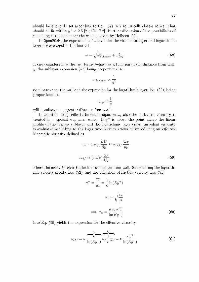
The physical domain is divided into control volumes that must ful�ll some require-ments such as they are never negative and they must completely �ll the solutiondomain. An example of two cells is shown in Figure 5.

All values are solved in the cell centers (points P and N). The terminology usedin OpenFOAM is used here which will make the derivation of the numerical schemes

24

Figure 5: Cell in OpenFOAM.

more understandable. Cells are connected by faces. Each face is owned by oneadjacent cell and the other cell is called the neighboring cell. The face f has an area|Sf | and a unit normal vector n pointing towards the neighbor. Thus a surface areavector is de�ned as

Sf = |Sf |n

The vector d points from the center of the owner cell to the center of the neighborcell

d = PN (64)

The vector Pf points from the center of the owner cell to the center of face f and thevector Nf from the center of the neighbor cell to the center of face f . The volumeof the owner cell is de�ned as VP .

The cells are not ordered in any way and they are connected to each otherthrough the faces only, not by any special indexing system. Such a mesh is calledunstructured. [23]

3.2 Equation Discretization

A general form of a transport equation is used to present how di�erent terms aretransformed from the di�erential forms into the discrete form.

∂φ

∂t+∇ · (Uφ) = ∇ · (α∇φ) + qφ (65)

25

In order to discretize the equation according to the �nite-volume approach, theequation is integrated over a control volume V to obtain.

time derivative︷ ︸︸ ︷∫V

∂φ

∂tdV +

convection term︷ ︸︸ ︷∫V

∇ · (Uφ) dV =

diffusion term︷ ︸︸ ︷∫V

∇ · (α∇φ) dV +

source term︷ ︸︸ ︷∫V

qφ dV (66)

The integration of the time derivative and the source term is straightforward. Theterms are simply multiplied by the cell volume VP . There are several ways forapproximating the time derivative itself. The simplest one is the implicit Eulermethod where the time derivative is approximated as∫

V

∂φ

∂tdV ≈ (φV )n+1 − (φV )n

∆t(67)

where n is the readily solved time level and n+1 the time level in which the variablesare being solved. The method is �rst-order accurate in time but unconditionallystable. The more accurate option is the backward method given as∫

V

∂φ

∂tdV ≈ 3(φV )n+1 − 4(φV )n + (φV )n−1

2 ∆ t. (68)

The backward method is second-order accurate in time with the cost of higherrequirements for memory due to the need to store the solution from two previoustime levels (n and n− 1) [20].

The integration of convection and di�usion terms needs a special attention. TheGauss divergence theorem is applied on them which, in its general form, can bewritten as [18, Ch. 16.4] ∫

V

∇ ? φdV =

∫S

φ ? dS (69)

where φ is a (smooth) tensor �eld, ∇? represents any of the derivatives ∇· (diver-gence), ∇× (curl) or simply ∇ (gradient). Surface S is closed and encloses thevolume VP and dS is the surface vector pointing out from the volume VP . Apply-ing the Gauss theorem on the convection term the outer divergence operation willvanish and the volume integral will be turned into a surface integral∫

V

∇ · (Uφ) dV =

∫S

φU · dS (70)

By further approximating the surface integral by a sum over �nite discrete parts,Sf , of surface S, the convection term becomes∫

V

∇ · (Uφ) dV =

∫S

φU · dS ≈∑f

φU · Sf (71)

26

Similar steps can be taken with the outer divergence operation in the di�usion term.The discrete form of the transport equation is then obtained as

VP∂φ

∂t+∑f

φU · Sf =∑f

(α∇φ) · Sf + VPqφ (72)

Since the volume integral is turned into a surface integral the variables (U, α, φ,∇φ)need to be expressed on the surfaces, too. Since they are normally expressed incell centers, a need for interpolation arises. There are several ways to interpolatevariables. In the following, three schemes are introduced.

3.2.1 Linear interpolation

Linear Interpolation or Central Di�erencing means that the value φ is interpolatedonto the face by weighting the two adjacent cell center values by their distances tothe face

φf ≈ wφP + (1− w)φN (73)

so that the weight factor (w) is the ratio of the neighboring cell center distance tothe face and to the owner cell center [23]

w = fN/PN (74)

Central di�erencing is symmetrical and is used in the discretization of di�usionterms. It is, however, unbounded which means that non-physical new minimum ormaximum values may arise due to interpolation. At the worst, this may lead to un-stable computation which usually prevents its usage in conjunction with convectiveterms.

Looking at the truncation error in a one-dimensional non-equally spaced mesh(Figure 6), expressing φ in points P and N , and by developing it into a Taylor series

Figure 6: Set-up for studying truncation errors.

around the face f yields

φP = φf − d1∂φ

∂x+d2

1

2

∂2φ

∂x2− d3

1

6

∂3φ

∂x3+d4

1

24

∂4φ

∂x4+O(d5

1) (75)

φN = φf + d2∂φ

∂x+d2

2

2

∂2φ

∂x2+d3

2

6

∂3φ

∂x3+d4

2

24

∂4φ

∂x4+O(d5

2) (76)

27

Substituting φP and φN into Eq. (73) yields

φf ≈ wφP + (1− w)φN = φf + d1d21

2

∂2φ

∂x2+O(d3

1) +O(d32)︸ ︷︷ ︸

Truncation error

(77)

The leading term in the truncation error is proportional to second spatial derivativeof φ (∂

2φ∂x2 ) and to d1d2 which means that the method is second-order accurate in

space. If the cell size is halved the leading term of truncation error reduces to onefourth of the initial magnitude.

3.2.2 Upwind Interpolation

Another simple interpolation scheme is the Upwind interpolation. It is used in thediscretization of the convection term and can be thought to represent the transport-ing nature of the term. As the name implies it needs information on which side ofthe face is on the upwind or upstream side. In the convection term, there is alwaysthe convecting �ux (usually surface normal velocity) and the convected variable φ. Itis the convected variable that is interpolated with the upwind scheme. The upwindinterpolation of φ is written as

φf =

{φP ,Uf · Sf ≥ 0

φN ,Uf · Sf < 0(78)

Eq. (78) can be written in the same form as Eq. (73). Then the the weight factor is

wupwind =

{1 ,Uf · Sf ≥ 0

0 ,Uf · Sf < 0(79)

The upwind interpolation is bounded so that it can never produce oscillations [23].In the case of a positive convective velocity one can use Eq. (75) to study the

truncation error of the upwind interpolation.

φf ≈ φP = φf −d1∂φ

∂x+d2

1

2

∂2φ

∂x2+O(d3

1)︸ ︷︷ ︸Truncation error

(80)

The truncation error consists of a �rst-order term in addition to a similar sec-ond -order term that was present in the truncation error of the linear interpolationmethod. The �rst-order term is proportional to ∂φ

∂xand is thus damping or di�usive

in its nature so that it tends to smooth out any local peaks in the values of φ. Beinga �rst-order term it is also larger than the truncation error of the linear interpola-tion method which makes the upwind method usually too inaccurate to be used forobtaining a reliable �nal result. Due to its robustness it can be used for startingcomputations, however.

28

3.2.3 Blended Interpolation

A combination of central- and upwind interpolations can be formulated as

φf = (1− γ)(φ)upwind + γ(φ)CD (81)

where γ is a blending coe�cient [23]. This formulation o�ers a possibility to improvethe accuracy from that of the upwind scheme but still maintain stability.

In the blended di�erencing the value of γ is a constant. There are, however,methods that locally determine γ so that new extreme values are avoided with as highan accuracy as possible. The local value for γ is calculated based on the �ow �elditself. There are a range of such limiters in OpenFOAM such as the limitedLinear

scheme and many more in literature (see for example Hirsch [24, Ch. 21.3]) such asminmod and van Leer to mention a few.

The truncation error of the blended scheme consists of those of the upwindand linear schemes. Thus it includes a �rst-order term that is scaled according tothe value of γ which makes the scheme more di�usive compared with the linearinterpolation, but also improves stability [23].

3.3 The SIMPLE-algorithm

The Semi-Implicit Method for Pressure Linked Equations (SIMPLE) is a commonmethod for �nding a solution to the continuity- and momentum equations in par-ticular in incompressible cases. A traditional description of the algorithm is givenby Patankar [25] and the description in this chapter follows the implementation inOpenFOAM. The solution algorithm is very similar in both steady-state and time-accurate cases with moving meshes. In a time-dependent case, the algorithm is usedinside each time step while in a steady-state solution it can be used as such. Thesolver used in the steady-state computations is simpleFoam and the time-accuratesolver is pimpleDyMFoam. The name of the time-accurate solver stands for a com-bination of the PISO-algorithm, that is a common method for solving time-accurateproblems [26], and of the SIMPLE-algorithm. The code allows the use of dynamicmeshes, which is expressed by the part DyM in the name. The two codes have somedi�erencies that will be pointed out in the following derivation.

First, the momentum equation is formed. Each term in Eq. (16) is discretizedby integrating over a control volume (VP ) and applying the Gauss law, Eq. (69), totransform the volume integrals into surface integrals.

time derivative︷ ︸︸ ︷∂U

∂tVP +

conv︷ ︸︸ ︷∑f

φfUf −∑f

νfSf

1.diff︷ ︸︸ ︷

(∇U)f +

2.diff︷ ︸︸ ︷(∇U)Tf −

1

3tr(∇U)T I

= Q−

RVP

∇p dV︷ ︸︸ ︷∑f

(Sfp)

(82)where

φf = Uf · Sf (83)

29

is the volume �ux through face f that is obtained at the end of the iteration processor, if no previous loop has been conducted, by a linear interpolation of cell-centervelocities. If the MRF method is applied the volume �ux is expressed in the relativecoordinate system as discussed in Chapter 2.3. In the case of a moving mesh, φf isrelative to mesh motion

ω × r · Sf . (84)

The velocity gradient tensors are not yet in their discrete form nor is the timederivative for the sake of a clearer presentation. In Eq. (82), only the surface areavector Sf and the volume �ux φf are, by de�nition, known on cell faces. Theface values of other variables must somehow be approximated from their cell-centervalues. The e�ective viscosity νeff was chosen to be linearly interpolated whichre�ects the symmetric nature of di�usion.

The calculation of the viscosity term is divided into two parts since the treatmentof the velocity gradient tensor di�ers between them in the code. In the �rst term,denoted by 1. di�, a part of the gradient (the orthogonal part) is computed directlyfrom face adjacent cell-center values

(∇U)f =Un −Uo

d(85)

This is a good approximation if the vector d that connects the cell centers is parallelto the surface area vector Sf . If the vectors are not aligned, however, velocitygradients computed in the cell centers are used as a correction term. In order toconstruct the correction term, the cell-center velocity gradients are computed usingthe Gauss law

∇U =1

VP

∑f

SfUf (86)

where the velocities are interpolated onto the cell faces according to the linear in-terpolation method. The velocity gradients in the second part of the di�usion term(2. di� ) are �rst computed in cell centers according to Gauss law, Eq. (69), andthen linearly interpolated onto the faces. Also the pressure gradient is computed bylinearly interpolating the cell-center values onto the cell faces. The time derivativeis non-zero only in time accurate computations and can be approximated by usingany of the schemes presented in Chapter 3.2. The source term Q = qVP can containany volume force (per unit mass) such as gravity or electromagnetic forces. If themoving reference frame (MRF) is activated, the additional source term

ω ×UIVP (87)

is also included in Q. Eq. (82) stands for force balance in one control volumeVP . Writing a similar equation for each cell leads to a set of equations with asmany equations as there are cells. The set of equation can be presented as a matrixequation. Splitting the left-hand-side into diagonal and o�-diagonal contributionsand writing the equation for only one cell gives

APUP +∑n

AnUn = RHS (88)

30

where AP stands for the diagonal term and An for the o�-diagonal terms in onerow of the (n × n) coe�cient matrix A. The diagonal term (AP ) multiplies thevelocity UP that the equation is written for. Accordingly, the o�-diagonal terms (An)multiply the velocities of the neighboring cells Un which gives a more understandablemeaning to the matrix coe�cients: the diagonal term represents the contribution ofthe cell itself on the new value to be solved, and the o�-diagonal terms contain thecontributions of the neighboring cells. The fact that usually only up to the secondneighbours are included in each equation (e.g. in ∇U-term) explains the fact thatthe coe�cient matrix is quite sparse i.e. most of its terms are zero. The term RHScontains all explicit terms in Eq. (82) which includes among others the second partof the di�usion term and the pressure gradient as such.

Before solving the momentum equation the matrix equation is under-relaxedin order to increase the diagonal dominance of the coe�cient matrix and improvecomputational stability. If the coe�cient matrix is not diagonally dominant

AP <∑n

An

the diagonal term is �rst replaced by the sum of the o�-diagonal terms and a corre-sponding term ∑

n

An − AP

is added onto the right-hand-side of the equation. The actual under-relaxationmeans that the diagonal terms AP are divided by a relaxation factor 0 < αU ≤ 1. Acorresponding term is added to the right-hand-side to keep the equation valid, andthus the momentum equation becomes

APαU

UP +∑n

AnUn = RHS +(1− αU)

αUAPUP (89)

from which a new velocity can be solved.In order to de�ne the pressure equation, new de�nitions are needed. Firstly,

the pressure dependent part is removed from the right-hand-side of the momentumequation (RHS). The pressure gradient is not written in its discretized form for thesake of clarity

RHS = rhs−∇p VP . (90)

Furthermore, a so called H-operator is de�ned as

H(U) =rhs−

∑nAnUn

VP(91)

and the diagonal term is divided by the cell volume VP .

aP =APVP

(92)

Dividing Eq. (88) and substituting de�nitions (90), (91) and (92) gives

aP UP = H(U)−∇p. (93)

31

Dropping out the pressure gradient, a velocity-like term and a corresponding volume�ux are obtained. They are denoted by an upper index ∗

U∗ =H(U)

aP(94)

φ∗f = U∗f · Sf (95)

The linear interpolation of U∗ is used to obtain the �ux φ∗f on each face. If the MRFis active φ∗f is expressed in the relative coordinate system by subtracting the term

(ω × r) · Sf .

Substituting U∗ back into Eq. (93) and dividing by aP gives an expression forvelocity

UP = U∗ − ∇paP

(96)

The continuity equation, Eq. (9), states that the velocity �eld has no divergence.Taking the divergence of Eq. (96) leads to an expression between the velocity andpressure.

∇ ·UP = ∇ ·U∗ −∇ ·(∇paP

)= 0

=⇒ ∇ ·(∇paP

)= ∇ ·U∗

Both divergence terms are discretized using the Gauss law (Eq. 69)∑f

((

1

aP)f (∇p · Sf )f

)=∑f

φ∗f (97)

The coe�cient1

aP

that comes from the coe�cient matrix of the momentum equation and is stored foreach cell, is interpolated onto the faces using the linear interpolation. The surfacenormal pressure gradient

∇p · Sfis evaluated partly in an explicit and partly implicit manner like the �rst part of thedi�usion term in the momentum equation (see Eqs. (85) and (86)).

To account for the explicit non-orthogonality correction, the pressure equation(97) is repeated several times. After solving the pressure equation, a new volume�ux φf is obtained by subtracting a �ux term (Fp) obtained from the actual discretepressure equation based on Eq. (97) from φ∗f , so that φf has zero divergence i.e. theconvective �ux exactly ful�lls the continuity constraint.

φf = φ∗f − Fp (98)

32

After obtaining �ux φf , the pressure is explicitly under-relaxed as

pn+1 = αpp+ (1− αp)pn (99)

Finally, a new velocity is obtained by correcting U∗ with the latest pressure gradient

Un+1 = U∗ − 1

aP∇pn+1 (100)

3.4 Linear Solvers

The matrix equations arising from the governing equations are typically sparse inCFD. In this Chapter, solution methods for a general matrix equation, written as

Aφ = Q (101)

are presented mainly by following the description by Ferziger and Peri¢ [20]. Sincethe matrices are sparse, they are solved iteratively and for which there is a range ofdi�erent algorithms available. Two solvers, the preconditioned biconjugate gradient(PBiCG) and the generalized geometric-algebraic multi-grid (GAMG), are used inthe computations presented in this study. The PBiCG method is used for solvingthe equations for velocity and turbulence quantities, and the GAMG for the pressureequation.

The idea of conjugate gradient methods is that solving the matrix equation isreformulated as a minimization problem of a function F .

F =1

2φTAφ− φTQ (102)

The minimum is searched for by �nding minima in one direction at a time. Alldirections can be thought to be perpendicular to all preceeding directions and theerror is reduced on every iteration. In theory there are as many linearly indepen-dent directions as there are equations (rows) in the matrix equation. The rate ofconvergence depends on the condition number

κ =λmaxλmin

(103)

of the coe�cient matrix A where λmax and λmin are the largest and the smallesteigenvalues of the matrix. The condition number is often very large in CFD appli-cations and manipulating it allows to improve convergence. The condition numbercan be reduced by multiplying the original equation by some matrix so that thesolution of the equation is not changed but the eigenvalues of the matrix are. Thisstep is called preconditioning.

Conjugate gradient methods are only applicable for symmetric matrices which isnot the case if upwind biasing is used in the discretization procedure. To overcomethis problem, unsymmetric systems are turned into symmetric ones for example by

33

creating a larger system of equations from the original coe�cient matrix A and itstranspose AT (

0 AAT 0

)(φ

φ

)=

(Q0

)(104)

where φ plays no role. The size of the matrix is increased but symmetry is achieved.Pressure equation is solved using GAMG. In GAMG the idea is that the solver

starts solving the matrix equation from the �nest grid level which corresponds tothe computational grid. The grid is �rst coarsened step by step and then re�nedwhile the equations are solved on each grid level. There are also several possibilitiesfor how to do the mapping both from a �ner to a coarser grid level (restriction)and the other way around (prolongation). The bene�t of using several grid levels isthat the solution is considerably faster on the coarser grid levels. Furthermore, thesolution on a coarser grid level e�ciently takes out large-scale errors. Provided thatthe bene�ts due to an improved convergence are greater than what mapping thesolution between grid levels and creating grids costs in time, the use of the GAMGmethod is justi�ed. Clearly, the bene�ts grow with a growing computational grid.

Before mapping any solution from one grid level to another, the solution shouldbe smooth. This is ensured by using an iterative method that produces smoothsolutions. According to Ref. [20, Ch. 5.3.8], it does not play a critical role whichmethods are used, provided that the method ful�lls certain conditions. In particular,with elliptic equations such as the pressure equation, using basic iterative methodson the �nest level only is ine�ective due to properties related to the eigenvalues ofsuch problems. Thus GAMG is a good choise for solving the pressure equation andalso OpenFOAM documentation recommends to do so.

34

4 Steady Computations with a Single Blade

The �rst computations are conducted in the simplest possible case. One propeller inopen-water conditions is analysed as a steady-state problem with periodic boundaryconditions so that only one of the �ve blades is included in the grid. There is mea-sured data of thrust and torque coe�cients, KT and KQ, with 14 values of advancecoe�cient J for validation of the computed results. This case is extensively used toevaluate the correctness of boundary conditions, solver settings and discretizationschemes. As a result, a computational set-up is �xed and subsequently throughlytested. This chapter includes a documentation of the testing phase while initialcomputations are omitted for the sake of a clearer presentation. The settings testedwill be used as a basis in the more demanding cases where trial and error would bemore expensive.

The computational domain consists of a volume around one blade. The completepropeller with hub is shown in Figure 7. The part inside the periodic domain is

Figure 7: The complete propeller with the part included in the periodic grid coloredin blue.

colored in blue while the grey color represents the rest of the propeller. The caseset-up of the periodic computation is shown in Figure 8. The periodic boundaries,shown in grey, are identical with each other. Inlet and outlet boundaries of themesh are de�ned as separate patches so that boundary conditions can be de�ned onthem. Furthermore, the hub and the surrounding boundary (cavitation tunnel wall)

35

are de�ned as separate parts of the mesh boundary.The surface grid on the propeller is shown in Figure 9. The grid is re�ned close to

the leading and trailing edges while the �atter parts of the blade surface are coarser.In order to achieve a better mesh quality, there is a band that follows the leading andtrailing edges that allows the construction of a more regular structure of the surfacemesh in those regions. Figure 10 shows the volume mesh around the propeller. Thesub�gures illustrate the internal mesh at di�erent radial positions around the blade.The mesh is mostly tetrahedral but, close to the propeller surface, there are twentyprismatic layers that ensure a su�cient mesh density inside the boundary layer. Theboundary layer mesh is best shown in sub�gure d) but is present everywhere on theblade surface.

4.1 Boundary Conditions

At the inlet, velocity is �xed to give a desired advance coe�cient J . As described inChapter 1.4.1, the advance coe�cient in measurements was evaluated from a velocitymeasured 150 mm upstream from the propeller plane at a distance of 60 mm fromthe tunnel wall. Thus reaching exactly the same J value as in measurements wasnot possible which was, however, accounted for by evaluating an individual advancecoe�cient in each computation. As can be seen in Figure 11, the J values correspondquite well to the measured ones.

The turbulence quantities were estimated at the inlet by setting turbulence in-tensity between

0.5% < I =

√23k

|Uinlet|< 1% (105)

and turbulence viscosity ratio approximately

νTν

=k

νω≈ 10 (106)

which gives the boundary conditions

k = 0.001 m2/s2 (107)

ω = 100 s−1. (108)

Turbulence handling near walls is as described in Chapter 2.4.The surface normal gradient of pressure is set to zero (∇p · Sf = 0) at all

boundaries except for the outlet where pressure is �xed to be zero (p = 0 m2/s2).Thus, it is the relative (or gauge) pressure that is solved for, which is additionallyscaled by density as discussed earlier. All other quantities have the numerical zero-gradient condition at the outlet in order to keep the computation well de�ned.

The hub and the tunnel walls were de�ned as frictionless walls. The velocitycomponent normal to the wall is set to zero in order to prevent �ow through it.The velocity component parallel to the surfaces and all other variables have thezero-gradient condition.

36

(a) Outer boundaries.

(b) A view with the foremost periodic boundaries hidden.

(c) A closer view on the propeller and hub.

Figure 8: The case set-up in the steady-state computations with one blade only.Boundary names are given in part b).

37

(a) The view from the upwind direction. (b) The view from the leading edge.

(c) The view from the trailing edge. (d) The view from the downwind direction.

Figure 9: Surface grid on the propeller surface.

4.2 Results

The case was computed with several discretizations. Most of the results are notpresented here, since they only served as initial tests to give understanding of howdi�erent settings a�ect the computation. With most settings, the force coe�cientswere within 2 % of each other which tentatively implies that the mesh is adequateand the computation is also otherwise set up correctly.

4.2.1 Force Prediction

With a �xed computational set-up, the performance of the settings was evaluated bycomparing the thrust and torque coe�cients, KT and KQ, against the experimentaldata over a range of operating points (see Figure 11). Since the correct advance co-e�cient was di�cult to set precisely and the computational results are not in perfectcorrespondence with the experimental data, an individual advance coe�cient wascalculated for each computation. The velocity was probed at the location where itis measured with a Prandtl tube in the test facility. By eye, one can draw a con-clusion that the results at lower J-values are often slightly overpredicted comparedto the experimental data. The evaluation of J , however, reduces the overprediction.All forces lie within 3 percent of the experimental data except for the lowest value

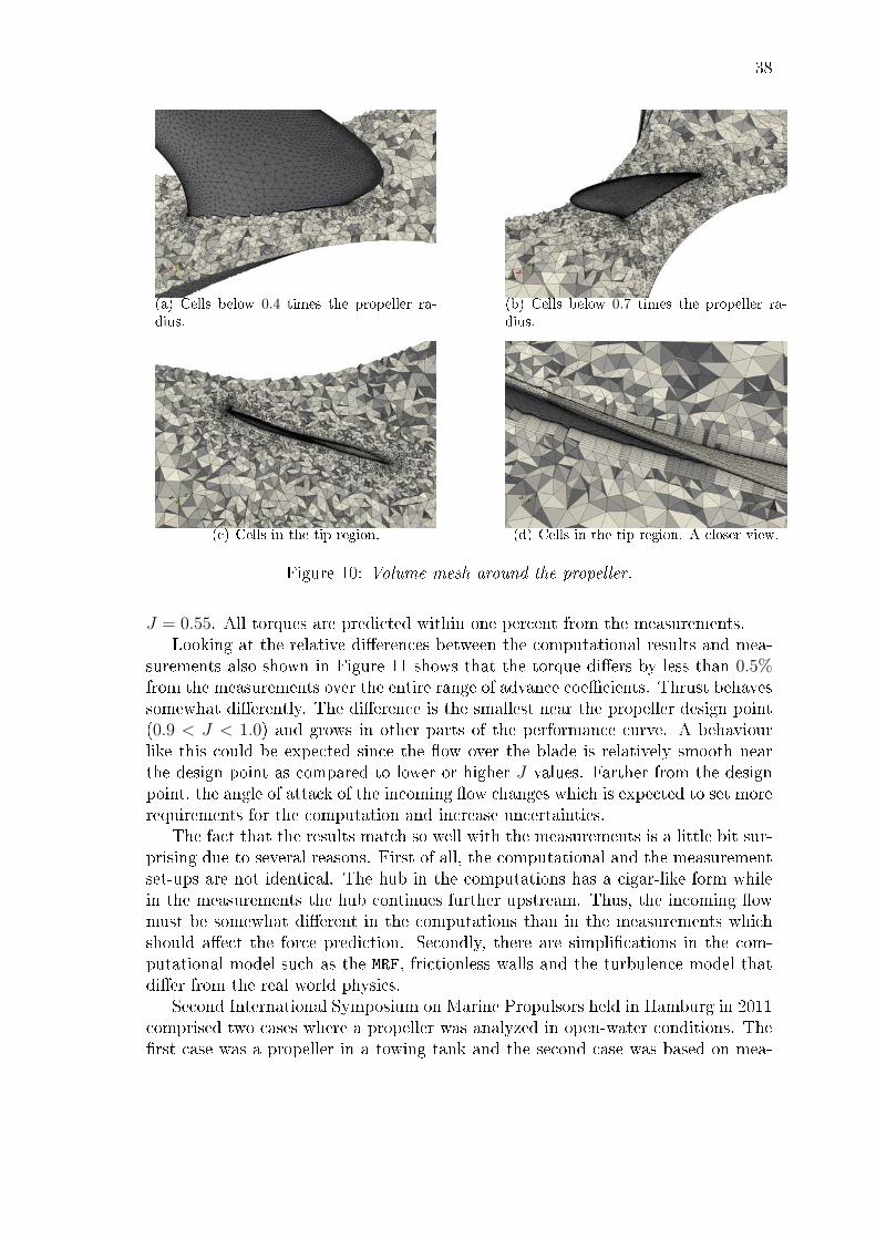
38

(a) Cells below 0.4 times the propeller ra-dius.

(b) Cells below 0.7 times the propeller ra-dius.

(c) Cells in the tip region. (d) Cells in the tip region. A closer view.

Figure 10: Volume mesh around the propeller.

J = 0.55. All torques are predicted within one percent from the measurements.Looking at the relative di�erences between the computational results and mea-

surements also shown in Figure 11 shows that the torque di�ers by less than 0.5%from the measurements over the entire range of advance coe�cients. Thrust behavessomewhat di�erently. The di�erence is the smallest near the propeller design point(0.9 < J < 1.0) and grows in other parts of the performance curve. A behaviourlike this could be expected since the �ow over the blade is relatively smooth nearthe design point as compared to lower or higher J values. Farther from the designpoint, the angle of attack of the incoming �ow changes which is expected to set morerequirements for the computation and increase uncertainties.

The fact that the results match so well with the measurements is a little bit sur-prising due to several reasons. First of all, the computational and the measurementset-ups are not identical. The hub in the computations has a cigar-like form whilein the measurements the hub continues further upstream. Thus, the incoming �owmust be somewhat di�erent in the computations than in the measurements whichshould a�ect the force prediction. Secondly, there are simpli�cations in the com-putational model such as the MRF, frictionless walls and the turbulence model thatdi�er from the real world physics.

Second International Symposium on Marine Propulsors held in Hamburg in 2011comprised two cases where a propeller was analyzed in open-water conditions. The�rst case was a propeller in a towing tank and the second case was based on mea-

39

surements of the same propeller in a cavitation tunnel. More detailed descriptions ofthe results are described in Ref. [27]. Apart from di�erent measuring equipment, thehub geometries di�ered between the cases and the measured forces in the cavitationtunnel case had no e�ects due to cavitation. The measured thrusts di�ered betweenthe two cases by only about 1%, so the e�ect of the experimental set-up seems notto be very dominant. Thus, the force prediction presented in this chapter is credibleand shows that the computational model used reproduces propeller forces within anaccuracy of a few percent. Furthermore, it also predits the trends properly with avarying advance coe�cient and is in line with results presented in literature that arebased on similar computational methods.

(a) Absolute values of KT and KQ as com-pared against experimental data over a rangeof advance coe�cient values J .

(b) Relative errors of the thrust- and torquecoe�cients relative to measurements over arange of advance coe�cient values J .

Figure 11: Open-water performance.

4.2.2 Distributions on the Blade Surface

Three operating points, J = 0.65, J = 0.90 and J = 1.15, are inspected in moredetail. The pressure coe�cient (Cp) distributions on the pressure- and suction sideswith all three values of J are presented in Figure 12. Clearly, the loading is largerat the lower J-values which is in line with general knowledge and the open-watercurve (Figure 11). The forces acting on propeller increase with a decreasing advancecoe�cient.

Turbulent viscosity (νT ) scaled by the molecular kinematic viscosity ν at a dis-tance of 0.5% times the propeller diameters from the blade surface is given in Figure13. In an incompressible �ow, the turbulent viscosity is the only turbulence variablethat shows up in the conservation equation for momentum (or continuity). It actsthrough the di�usion term and increases the viscous forces. The turbulent viscosityseems to increase with an increasing advance coe�cient J on the pressure side of theblade and to decrease on the suction side of the blade. This is explained by the factthat the stagnation point moves towards the pressure side when J decreases. Thusat a low J , the �ow is smoother on the pressure side, but passes a tighter turn overthe leading edge before reaching the suction side which can be seen as an increasedtendence to turbulence. With an increasing J , the opposite happens.

40

Figure 14 shows wall bounded streamlines on the propeller blade. The surfacesare colored by the friction factor (Cf ), that is based on the magnitude of the wallshear stress. The streamlines show that the �ow separates close to the trailing edgewith all of the three advance coe�cients. The separation is shown as a divide in thestreamlines and is present on both the suction and pressure side of the propeller.With a decreasing advance coe�cient, the tendence for separation on the suction sideseems to increase which is expected due to the increased angle of attack of the blade.Apart from areas close to the trailing edge, the �ow stays attached to the surface. Itcould be that the separation should increase more with advance coe�ents far fromthe design point of the propeller and that the current method fails to reproduce thebehaviour. It would explain the di�erences in the errors of the force coe�cients witha varying J . A more detailed analysis would require experimental data on the �ow�eld.

41

(a) J = 0.65, suction side. (b) J = 0.65, pressure side.

(c) J = 0.90, suction side. (d) J = 0.90, pressure side.

(e) J = 1.15, suction side. (f) J = 1.15, pressure side.

Figure 12: Pressure coe�cient Cp on the blade surface.

42

(a) J = 0.65, suction side. (b) J = 0.65, pressure side.

(c) J = 0.90, suction side. (d) J = 0.90, pressure side.

(e) J = 1.15, suction side. (f) J = 1.15, pressure side.

Figure 13: Turbulent viscosity ratio νT/ν on the blade surface.

43

(a) J = 0.65, suction side. (b) J = 0.65, pressure side.

(c) J = 0.90, suction side. (d) J = 0.90, pressure side.

(e) J = 1.15, suction side. (f) J = 1.15, pressure side.

Figure 14: Friction factor Cf and streamlines on the blade surface.

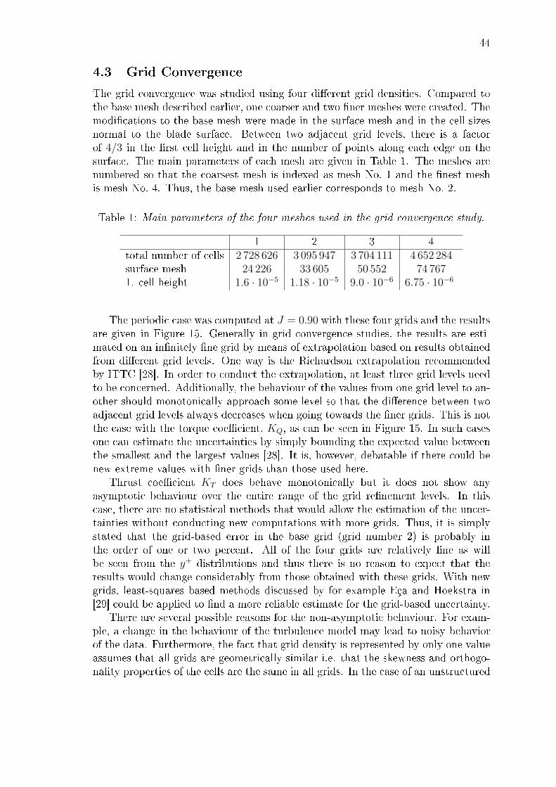
44

4.3 Grid Convergence

The grid convergence was studied using four di�erent grid densities. Compared tothe base mesh described earlier, one coarser and two �ner meshes were created. Themodi�cations to the base mesh were made in the surface mesh and in the cell sizesnormal to the blade surface. Between two adjacent grid levels, there is a factorof 4/3 in the �rst cell height and in the number of points along each edge on thesurface. The main parameters of each mesh are given in Table 1. The meshes arenumbered so that the coarsest mesh is indexed as mesh No. 1 and the �nest meshis mesh No. 4. Thus, the base mesh used earlier corresponds to mesh No. 2.

Table 1: Main parameters of the four meshes used in the grid convergence study.

1 2 3 4total number of cells 2 728 626 3 095 947 3 704 111 4 652 284surface mesh 24 226 33 605 50 552 74 7671. cell height 1.6 · 10−5 1.18 · 10−5 9.0 · 10−6 6.75 · 10−6

The periodic case was computed at J = 0.90 with these four grids and the resultsare given in Figure 15. Generally in grid convergence studies, the results are esti-mated on an in�nitely �ne grid by means of extrapolation based on results obtainedfrom di�erent grid levels. One way is the Richardson extrapolation recommendedby ITTC [28]. In order to conduct the extrapolation, at least three grid levels needto be concerned. Additionally, the behaviour of the values from one grid level to an-other should monotonically approach some level so that the di�erence between twoadjacent grid levels always decreases when going towards the �ner grids. This is notthe case with the torque coe�cient, KQ, as can be seen in Figure 15. In such casesone can estimate the uncertainties by simply bounding the expected value betweenthe smallest and the largest values [28]. It is, however, debatable if there could benew extreme values with �ner grids than those used here.

Thrust coe�cient KT does behave monotonically but it does not show anyasymptotic behaviour over the entire range of the grid re�nement levels. In thiscase, there are no statistical methods that would allow the estimation of the uncer-tainties without conducting new computations with more grids. Thus, it is simplystated that the grid-based error in the base grid (grid number 2) is probably inthe order of one or two percent. All of the four grids are relatively �ne as willbe seen from the y+ distributions and thus there is no reason to expect that theresults would change considerably from those obtained with these grids. With newgrids, least-squares based methods discussed by for example Eça and Hoekstra in[29] could be applied to �nd a more reliable estimate for the grid-based uncertainty.

There are several possible reasons for the non-asymptotic behaviour. For exam-ple, a change in the behaviour of the turbulence model may lead to noisy behaviorof the data. Furthermore, the fact that grid density is represented by only one valueassumes that all grids are geometrically similar i.e. that the skewness and orthogo-nality properties of the cells are the same in all grids. In the case of an unstructured

45

grid this is not the case, which re�ects on the results [29]. As an example, non-orthogonalities in the grid directly a�ect the computation of laplacian terms thatplay an important role in solving the pressure �eld. Pressure, on the other hand,dominates propeller forces.

The results may also change due to geometrical di�erences between the grids.Since the surface grid is di�erent on each grid level, also the surface area di�ersbetween the grids and the surface integration is performed di�erently with eachgrid. The di�erences in surface areas were found to be less than 0.2% between allof the grids so the in�uence of the area is quite negligible.

(a) Thrust coe�cient, KT . (b) Torque coe�cient, KQ.

Figure 15: Force coe�cients computed with four di�erent grids.

The y+ values in the �rst cells next to the wall play an important role in thequality of the results. In Figures 16 and 17, there are the distributions of the y+

values on the blade computed with all of the four grids on the suction and thepressure sides, respectively. With the �nest grid, the y+ values are well below oneso the surface normal density of the grid is adequate. Up to the second coarsest grid(grid number 3), y+ is mostly below 2, which is usually considered �ne enough. Inthe coarsest mesh, there are signi�cant regions where y+ > 2. The contours presentthe discrete distibutions of the values without any interpolation that would smooththe �eld in order to emphasize the di�erences in the grids.

The grid dependence study shows that there is dependence on the grid in thesolutions, but it is relatively small. The order of magnitude of the errors is approx-imately 1% and in the case of the torque coe�cient, it is even smaller. The errorbeing small, it can be expected that the base grid is adequate and similar meshescan be used to study the e�ects caused by a hybrid mesh and time discretization.

46

(a) Grid 1, suction side. (b) Grid 2, suction side.

(c) Grid 3, suction side. (d) Grid 4, suction side.

Figure 16: y+ on the suction side with four mesh densities at J = 0.90.

(a) Grid 1, suction side. (b) Grid 2, suction side.

(c) Grid 3, suction side. (d) Grid 4, suction side.

Figure 17: y+ on the pressure side with four mesh densities at J = 0.90.

47

5 Steady Computations with the Hybrid Mesh

The second computed case is the same as that analysed previously but the meshconsists of the two following parts:

• a cylidrical volume around the propeller with a mesh similar to that usedearlier (referred to as propeller mesh) and

• a hexahedral mesh around the propeller mesh (referred to as surroundings).

The propeller mesh was created with the same template as the mesh used earlierand consists, for the most part, of tetrahedral cells, but has prismatic cells in theboundary layer. The tetrahedral propeller mesh was cut close to the propeller sothat it con�nes a cylindrical volume. Both the MRF and the moving mesh requirethat the boundary faces of the propeller mesh have no component in the directionof the rotational movement so the cylindrical shape is adequate in that sense.

The surrounding mesh was created using snappyHexMesh that is part of theOpenFOAM distribution. A hole for the propeller mesh was left inside the surroundingpart so that the two separate meshes could be merged with the mesh handling toolsavailable in OpenFOAM. The hybrid mesh is illustrated in Figure 18.

(a) Propeller mesh. (b) Surrounding mesh around the propeller mesh.

Figure 18: Hybrid mesh.

One main objective in the computations with the hybrid mesh is to inspect howa discontinuity in the mesh with the Arbitrary Mesh Interface (AMI) between theregions a�ects not only the thrust and torque coe�cients, but also the propagation

48

of �ow structures downstream of the propeller. The correct propagation of the wakeis important when there are multiple propellers behind one another.

5.1 Stability

With the hybrid mesh, the computation was not as stable as earlier and di�erentdiscretizations were needed. The instability was traced back to the solution ofthe momentum equation. A stable computation was achieved by discretizing theconvection of momentum with the blended scheme with a ratio of 0.75 instead oflimitedLinear that was used earlier.The new method is more dissipative but alsoconsiderably more robust. Probably the main reason for the additional robustnessis the fact that the limiter does not depend on the solution itself as in the case ofthe limitedLinear scheme. Clearly, due to a greater contribution of the �rst-orderupwind, di�usivity is increased.

In order to evaluate the performance of the new settings, they were tested inthe periodic case and compared to earlier results and measurements. In Figure 19,there are iso-volumes of vorticity (∇ × U = 300 1

s) computed with the old and

the new settings. One can see that the new settings produce less vorticity. Thetip vortex is slightly thinner and also less vorticity emanates from the central partsof the blade. No considerable di�erence can be seen in the distance that the tipvortex is transported. The decrease in vorticity could be expected due to the higherdi�usivity of the new settings but these results imply that no dramatic losses arecaused in the prediction of propeller wake if the blended 0.75 scheme is used.

(a) Old settings (limitedLinear 0.33). (b) New settings (blended 0.75).

Figure 19: Iso-volumes of vorticity ω = 300 1sin the periodic case with the old and

the new settings. Colored by velocity magnitude.

In addition to the propagation of the tip vortex, also the force coe�cients wereevaluated with the new settings. They change from those computed with thelimitedLinear 0.33 scheme. The relative di�erences to both earlier results and tomeasurements (relative error) of the thrust and torque coe�cients, KT and KQ, at

49

J = 0.65, 0.90 and 1.15 are given in Tables 2 and 3, respectively. The force coe�-cients change by less than 1% from the previous results which can still be consideredacceptable concerning the overall accuracy of the simulation. In summary, the newsettings yield larger errors in the force coe�cients but they are, on the other hand,considerably more robust. Thus, they provide an adequate computational tool forthe purposes of this study.

Table 2: Comparison of thrust coe�cient, KT , computed with the blended 0.75

scheme (KT,BL) to that computed with the limitedLinear 0.33 scheme (KT,LL)and to the measured values (KT,M). Computations conducted with the periodic grid.

J Relative di�erence(

KT,BL−KT,LL

KT,LL

)Relative di�erence

(KT,BL−KT,M

KT,M

)0.65 0.81 3.500.90 0.40 0.641.15 0.86 1.24

Table 3: Comparison of torque coe�cient, KQ, computed with the blended 0.75

scheme (KQ,BL) to that computed with the limitedLinear 0.33 scheme (KQ,LL)and to the measured values (KQ,M). Computations conducted with the periodic grid.

J Relative di�erence(

KQ,BL−KQ,LL

KQ,LL

)Relative di�erence

(KQ,BL−KQ,M

KQ,M

)0.65 1.07 1.220.90 0.72 0.721.15 1.15 0.39

5.2 Comparison of MRF Domains

In order to further analyze how the MRF method is to be used, the hybrid mesh caseis computed using two di�erent MRF domains. In the �rst case, MRF is only appliedinside the propeller mesh, and, in the second case, it is active everywhere in themesh and thus similar to earlier computations. Figure 20 illustrates iso-volumes ofvorticity, ω = ∇×U = 300 1

sin order to track the tip vortex emanating from the

propeller. In the case illustrated on the right-hand-side, MRF is only applied insidethe propeller mesh and, in that region, the two solutions are very close to eachother. In the left-hand-side case where MRF is applied in the entire mesh, the tipvortex is transported through the mesh boundary. The mesh boundaries are shownas the shaded grey surfaces on the upstream and downstream sides of the propeller.A small change can be seen in the vortex when it penetrates the mesh boundary,but it is nevertheless transported through the interface quite nicely. If the MRF isdeactivated outside the propeller mesh, however, the vortex immediately dies at theboundary. It seems that the mesh interface itself does not a�ect the solution asmuch as the MRF boundary. The reason for the vortex dying at the MRF boundaryis discussed later.

50

(a) MRF method is applied in domain 2.Outer disturbances are not shown.

(b) MRF method is applied inside the propellermesh.

Figure 20: Iso-volumes of vorticity with the MRF method applied in two di�erentdomains.

The thrust and torque coe�cients computed with the hybrid mesh are shownin Figure 21. Applying the MRF only inside the propeller mesh yields lower thrustand torque coe�cients which, compared to measurements, have errors of 0.5 % and0.6 %, respectively. The results are also in line with the periodic computations withthe same settings. However, applying MRF everywhere with the hybrid mesh givesdi�erent results. The force coe�cients become larger and have errors of about 1.2 %(KT ) and 1.3 % (KQ).

In either computation, there are no signi�cant di�erences between single blades(approximately 0.1 %) which is expected and also an important implication of howwell the computational solution method works. The mesh introduces some asymme-try to the computation but the case itself is symmetrical so that all blades shouldyield the same results. Since the propeller mesh is identical around each blade, alldi�erences must be due to the numerical solution procedure and to the asymmetryin the surrounding mesh and the mesh interface. The variation in the coe�cientvalues between di�erent iterations is yet by an order of magnitude smaller.

51

(a) MRF method is applied in the entiremesh. Thrust coe�cient, KT .

(b) MRF method is applied inside the pro-peller mesh. Thrust coe�cient, KT .

(c) MRF method is applied in the entiremesh. Torque coe�cient, 10 KQ.

(d) MRF method is applied inside the pro-peller mesh. Torque coe�cient, 10 KQ.

Figure 21: Force coe�cients (KT and KQ) with the MRF method applied in twodi�erent domains at advance coe�cient J = 0.90.

Contours of tangential velocities at adjacent cross-sections behind the propellerare studied in order to see how the propeller wake propagates downstream. Anoverall picture of the contours under focus and their locations are shown in Figure22.

The cross-sections are shown separately in Figure 23. The �rst three contours atz = 0.025 m, z = 0.030 m and z = 0.035 m are from inside the propeller mesh andthe three latter contours at z = 0.045 m, z = 0.050 m and z = 0.055 m from thedownstream side of the propeller mesh boundary. In the �rst contours, there aresmall �ow structures near the blade tip that imply the existence of the tip vortex.Further downstream they gradually become weaker. The same trend can be seenin the overall �ow structure. Velocity peaks become smoother towards downstreamand thus the high velocity region grows and becomes more uniform. The resultsshown here are from the computation with MRF applied inside the propeller meshonly.

52

Figure 22: Cross-sections behind the propeller. The position of the propeller meshboundary is shown in green.

Tangential velocities at di�erent radial positions behind one propeller blade areplotted in Figure 24. The picture on the left-hand-side shows the velocities in thecase when the MRF is only applied inside the propeller mesh. In the right-hand-sidepicture, the MRF has been applied in the entire mesh. The location of the propellermesh boundary (and the MRF boundary in the �rst case) is shown as a vertical line(at z = 0.04 m). There is a slight notch in all of the velocity pro�les across the meshboundary but the overall form of the pro�les does not seem to be disturbed verymuch. Clearly, an interpolation at the mesh discontinuity must have some kind ofan e�ect on the velocities in a general case but the results show that it is not verylarge.

53

(a) z = 0.025 m. (b) z = 0.030 m.

(c) z = 0.035 m. (d) z = 0.045 m.

(e) z = 0.050 m. (f) z = 0.055 m.

Figure 23: Tangential velocities behind the propeller. MRF applied in the propellermesh.

54

(a) MRF applied in the propeller mesh. (b) MRF applied in the entire mesh.

Figure 24: Tangential velocities behind the propeller at several radial positions.

A much clearer trend can also be seen in the same �gure. When the MRF isactive the �ow �eld is convected by the relative velocity which is seen as a di�erentbehaviour of velocities at di�erent radial positions. In the case where MRF is onlyapplied inside the propeller mesh, it is the absolute velocity that convects �ow struc-tures outside of the propeller mesh. In that case the �ow is transported downstreammore or less as it is on the MRF boundary, since the axial velocity dominates overother components.

The same e�ect is seen in the velocity �elds at di�erent cross-sections. Thecontours from Figure 23 and corresponding contours from the case of the MRF appliedeverywhere are put together into Figure 25. The last three cross-sections in the twocases show the di�erent behaviour of the overall �ows. If MRF is applied, the �owrotates against the propeller rotation (counter clock-wise) when going downstreamwhich is caused by the relative velocity being responsible for convection. In the partwhere no MRF is applied, the rotation changes direction and is much weaker, hardlyvisible in still pictures. An animation makes the behaviour more apparent.

At the last cross-sections in both cases, the velocity �elds di�er from each other.In the case of MRF applied everywhere, the velocity di�erences are much smootherthan in the case of MRF applied only inside the propeller mesh. A possible reasonfor this is grid based di�usion that is stronger if the �ow direction is not alignedwith the cells. The mesh created with snappyHexMesh is aligned with the coordinateaxes (x, y, z), so removing MRF at the mesh boundary makes the �ow more alignedwith the cells and thus reduces numerical di�usion. On the other hand, numericaldi�usion only di�ers between the cases outside of the propeller mesh so it is probablynot the main reason for the di�erent results near the propeller. Figure 26 shows thatthe di�erence is present already inside the propeller mesh and upstream of it. Thetangential velocities are illustrated in both sides of the upstream side boundary ofthe propeller mesh and the di�erence seems to be present already upstream of thepropeller mesh. The di�erences in the velocities before the propeller mesh implythat the upstream side of the propeller mesh is probably not far enough from thepropeller which would cause the di�erences.

55

(a) MRF applied in the propeller mesh. (b) MRF applied in the entire mesh.

Figure 25: The e�ect of the MRF method on the propagation of �ow structures.

The propagation of the �ow reveals one interesting feature of the MRF. Lookingat the velocities at, say, the propeller mesh boundary, the solution corresponds toa situation where the propeller is in a di�erent position than what the modelledgeometry implies. The wake at the boundary looks like it is coming from a propellerthat has not rotated as much as the modelled propeller. Thus each cross-section,or in fact each point, corresponds to a di�erent propeller position and that positiondepends on the time that it takes for the �ow to come from the propeller to thatspeci�c point. When applying the MRF stops, the physics change abruptly so it isnot surprising that something happens to �ow structures such as tip vortex acrossthe boundary.

As a conclusion, the propagation of the �ow across the mesh boundary seemsto work nicely. An e�ect of a spatial change in the MRF method (stopping it orchanging it abruptly) is, however, not that simple and implies problems in steady-state CRP computations. Changes in the MRF source do a�ect the �ow downstreamof the propeller but also upstream of it. If possible, the upstream side of the MRF

domain should be as far as possible from the propeller to avoid any e�ects on the�ow around the propeller. In the case of a CRP, however, it is not possible to takethe boundary far from both propellers.

56

(a) MRF in the propeller mesh. z = 0.035 m. (b) MRF in the entire mesh. z = 0.035 m.

(c) MRF in the propeller mesh. z = 0.045 m. (d) MRF in the entire mesh. z = 0.045 m.

Figure 26: Comparison of velocities around the downstream side mesh boundary.

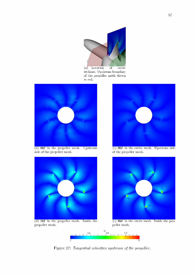
57

(a) Location of cross-sections. Upstream boundaryof the propeller mesh shownin red.

(b) MRF in the propeller mesh. Upstreamside of the propeller mesh.

(c) MRF in the entire mesh. Upstream sideof the propeller mesh.

(d) MRF in the propeller mesh. Inside thepropeller mesh.

(e) MRF in the entire mesh. Inside the pro-peller mesh.

Figure 27: Tangential velocities upstream of the propeller.

58

6 Time-Accurate Computations with the Hybrid Mesh

In this chapter, the same hybrid mesh that was described in Chapter 5 is used withthe time-accurate code pimpleDyMFoam. The boundary conditions are the same asearlier except for the propeller blades. They are de�ned as moving walls and themovement is de�ned to be the rotating movement.

The main focus in the time-accurate computations is to learn about errors arisingfrom temporal discretizations and how they depend on chosen settings. Three mainparameters that are expected to in�uence the temporal discretization are

• time discretization,

• time step size and

• the number of iterations inside one time step.

Increasing the number of iterations a�ects not only the accuracy but also increasesthe computational time. Therefore, it is important to �nd a number of iterationsthat gives an acceptable accuracy without spending too much time on unnecessaryiterations.

The time step size clearly a�ects the computational time required for a simulationover a certain time interval by a�ecting the number of taken time steps. On theother hand, the longer the time step the more iterations are needed inside each timestep, since the two adjacent solutions di�er more from each other.

The type of the temporal discretization a�ects the accuracy of the computationbut its e�ect on the simulation time is probably not very important. It does, howevera�ect the memory requirements considerably. Both the Euler and the backward timediscretizations are used and the number of iterations inside a time step is varied overa range from �ve to 40.

The open-water case is computed with three time steps corresponding to thefollowing propeller rotations:

• 0.5◦/∆t,

• 2◦/∆t and

• 5◦/∆t.

A clear motivation for the use of iterations inside a time step is given in Figure 28that illustrates the iso-surface of a Courant number of Co = 2 on the left-hand-sideand the isosurface Co = 10 on the right-hand-side. The maximum Courant numbersoccur at the propeller blade tip where the mesh is dense and velocities are high butthere are also regions with Co > 2 between the blades. These regions are causedby a denser region in the volume mesh that can be seen in the outer boundary ofthe propeller mesh also illustrated in the �gures. The maximum Courant numbersare approximately Co = 95 in the case of the smallest time step. With 2 degreesof propeller rotation per time step it is Co ≈ 375. The use of inner iterationsallows the introduction of under-relaxation also in the transient computation, which

59

considerably stabilizes the solution procedure. In order to use this kind of a gridand, at the same time, take the Courant number down to approximately Co = 1,the time step would need to be in the order of 0.005◦ propeller rotation per timestep, which would increase the number of time steps enormously.

(a) Courant number Co = 2. (b) Courant number Co = 10.

Figure 28: Isovolumes of Courant number.

The three parameters pose requirements to one another and they need to beconsidered as a whole in order to choose resonable settings. In the following, eachparameter is varied separately and resulting changes in the force coe�cients andin the wake �eld studied. Only one advance coe�cient, J = 0.90, is used in thetime-dependent case.

6.1 Force Prediction

The resulting force coe�cients are plotted against time in Figure 29. In each sub-�gure, the measured value is given as a solid horizontal line and the steady-stateresult from Chapter 5 is represented by the dashed horizontal line. The steady-stateresults are those computed with MRF applied in the entire grid.

The �rst two sub�gures illustrate the results with the smallest time step corre-sponding to 0.5◦ propeller rotation per time step. Both time discretizations yieldthe same average results. The backward-scheme gives more oscillations which isprobably due to its lower dissipation compared to the Euler method. The numberof iterations inside a time step does not a�ect the average results either which meansthat the error due to time discretization is not dominant compared to other factors.A further implication of a su�ciently accurate temporal discretization is the factthat the results are very close to the steady-state results computed with MRF appliedin the entire grid. These results are referred to as temporally converged results inthe following.

60

(a) Thrust coe�cient KT . Mesh movementper time step corresponds to 0.5◦.

(b) Torque coe�cient KQ. Mesh movementper time step corresponds to 0.5◦.

(c) Thrust coe�cient KT . Mesh movementper time step corresponds to 2◦.

(d) Torque coe�cient KQ. Mesh movementper time step corresponds to 2◦.

(e) Thrust coe�cient KT . E�ect of the timestep size.

(f) Torque coe�cient KQ. E�ect of the timestep size.

Figure 29: Force coe�cients (KT and KQ) against time at J = 0.90.

61

With a larger time step, 2◦ propeller rotation per time step, shown in the next twosub�gures, the time discretization plays a clear role. With an increasing number ofiterations inside a time step, the results approach the level obtained with the smallertime step (rotation of 0.5◦/∆t). Using ten iterations yields results that di�er fromthe temporally converged results by approximately two percent. With 20 iterations,the values are closer and with 40 iterations the results are the same as with thesmaller time step. Thus it seems that the numerical error due to time discretizationdoes not play a signi�cant role even with 2 degrees of rotation per time step but theerror due to insu�cient iteration (iterative error) does a�ect the solution.

If other parameters are kept constant the backward discretization predicts theforces better than the Euler discretization. This could be expected since the errorof the backward scheme is theoretically lower than that of the Euler scheme. Ac-cording to the conclusion that only the iterative error a�ects the forces with thetime step of 2◦ rotation per time step, not the numerical error, the di�erences in thenumerical errors should not explain the di�erence, however. Based on these results,the backward scheme seems to reduce the iterative error, too, compared to the Eulermethod. Thus, the results encourage to use the backward scheme whenever there isenough memory available.

The lowest sub�gures illustrate results with the three used time step sizes. Asmentioned earlier, the two smallest time steps yield the same average values, ifenough iterations are used inside a time step. A time step corresponding to apropeller rotation of 5◦ clearly underpredicts the forces with 40 inner iterations. Alarger amount of iterations might lead to better results but that was not tested. Thissubject will be further analyzed later with the conclusion that even a considerablylarger amount of iterations might not yield correct results.

An interesting trend is seen in the temporal variation of the forces. The larger thetime step the less oscillations there are in the results. The time discretization (thatwas just found not to a�ect solutions with su�ciently low time steps) �lters awayoscillations from the computations. This observation is in line with the theory. Thenumerical error damps oscillations and with an increased time step the numericalerror grows. Based on these observations, it can be concluded that the numericalerror in the case of 2◦ rotation per time step is small enough not to a�ect theaverage value of predicted forces but does still a�ect the temporal oscillations of theforces. Even if the results are the same with di�erent time step sizes provided that asu�cient amount of iterations are conducted within a time step, one thing needs tobe kept in mind. The case itself is probably not time-dependent, in particular in thesense of global forces. The time step determines the time scale of reproducable �owphenomena, since the time scale of events one is interested in must, of course, belarger than the time step used in order for the computation to be able to reproducethem. If there are structures on a smaller time scale in other cases such as theCRP-case the results should also have a stronger dependence on the time step size.

62

Table 4: Comparison of force coe�cients, KT and KQ, computed with moving mesh(0.5◦/∆t), backward discretization and ten inner iterations) and steady-state (MRFapplied everywhere).

KT 10KQ

steady-state 0.3005 0.6630time-accurate 0.3000 0.6625

Relative difference (%) 0.17 0.08

Compared to the steady-state results obtained with MRF applied everywhere inthe mesh, the time-accurate results are very similar. This fact was already seenqualitatively in Figure 29 but, for a quantitative comparison, the average valuescomputed with the smallest time step (0.5◦ rotation per time step), backward dis-cretization and ten inner iterations and those given by the steady-state computationare given in Table 4. The results di�er only by a fraction of a percent which is wellbelow the accuracy of the computations themselves. Thus the results are in linewith earlier computations and verify the correct usage and performance of the time-accurate code.

6.2 Convergence Within a Time Step

In order to better understand the connection between the time step size and conver-gence inside a time step, convergence histories of pressure inside one time step areplotted in Figure 30. The computations that yielded results una�ected by the timediscretization (temporally converged results) are plotted in green, and the computa-tions with errors in red. With a short time step, the residual level in the beginningof a time step is lower than in the case of a longer time step, and that level isindependent on the number of iterations conducted inside the time step. A longertime step seems not only to decrease the convergence rate but also the achievablelevel of accuracy inside a time step. These results show that the computation wherepropeller is rotated by 5◦ in a time step would probably not give good results evenwith a very large number of inner iterations.

It is di�cult to see from the residual histories when the iterative error no moreimpairs the solution. The residuals in cases of 0.5◦ rotation per time step with 5iterations are higher than the residuals with 2◦ rotation and 20 iterations. However,the results in the latter case have an error while the other results are good. Theredoes not seem to be any clear correlation between the residuals and the force predic-tion. It is, however, interesting to see that the convergence �rst reaches a maximalrate which then decreases with an increasing number of iterations. This impliesthat it might be bene�cial to have such a short time step that the convergence levelrequired to remove the e�ect of iterative error is reached during the fastest conver-gence, whatever the required level may be. A further optimisation of the solutionprocedure is left for further studies. For example, the use of a PISO-loop at the end

63

of a time step should decrease the iterative error but it was omitted in this studydue to stability reasons.

Figure 30: Residual histories of pressure.

6.3 Wake Prediction

The velocity �elds at 0.055 m behind the propeller (see the last cross-section inFigure 22) is shown in Figure 31. The �rst two contours are from the cases with0.5◦ rotation per time step that both reproduced the forces well. The �gure onthe left-hand-side should, with the smallest time step, backward time discretizationand 20 iterations per time step, theoretically be the most accurate out of all of thesix cases under consideration. There seem to be less velocity peaks in the wake,however, than in the less accurate case with only �ve iterations per time step (topright sub�gure).

The same trend can be seen in other sub�gures. The less iterations conductedwithin a time step the sharper velocity peaks there are in the wake (see 'middleleft' and 'middle right' sub�gures). Similarly, the longer the time step the strongerthe peaks are (see 'middle left' and 'bottom right' sub�gures). The numerical errorrelated to the time discretizations is di�usive in its nature so theoretically, a longertime step should yield a smoother velocity �eld. How the iterative error a�ects isnot that clear.

Comparing the cases with the Euler and backward schemes (see 'middle right'and 'bottom left' sub�gures) shows that the Euler scheme gives a smoother wakethan the backward scheme. By theory, this is expected since the error related to theEuler scheme should be more di�usive.

64

The streamwise propagation of the propeller wake is illustrated in Figure 32.The cases are the same as in Figure 31 and the same observations made based onFigure 31 are con�rmed by looking at any streamwise position behind the propeller.There is a possible explanation to the results that seemingly contradict with theory.A less di�usive (more accurate) computation is able to reproduce smaller �ow struc-tures that e�ectively smooth the �ow �eld. A numerical dissipation preventing such�ow structures can thus reduce mixing processes in the �ow and thus give sharpergradients in the propeller wake. The fact that there are less oscillations in the forcecoe�cients with longer time steps is in line with this explanation.

Anyway, even if the propeller forces may be correctly predicted with less accuratehandling of temporal changes, the wake may not be correctly reproduced with thesame settings. In a case of two propellers, the di�erences in the wake �elds certainlya�ect at least the distribution of forces at the aft propeller. Thus, they can alsoa�ect the global force prediction. The sensitivity of forces on the wake predictionneeds to be treated more carefully in the CRP computations. At this point it isonly clear that the forces on the front propeller do not directly indicate anything ofthe quality of the propeller wake.

In all cases in Figure 32, the mesh boundary can be seen in the �ow �eld,in particular in the outer part of the wake. No clear di�erences can be pointedout between di�erent numerical settings, however. Somehow the boundary isolatesstructures on its opposite sides. Based on these �gures, the mesh boundary doesnot seem to impair the solution too much but anyway attention must be paid onthe subject in the CRP computations.

The time-accurate code seems to work as expected. The force prediction is inline with the steady-state results and, even if the case itself is more or less steady,the e�ect of important parameters a�ecting the error of the temporal discretizationscan be seen. As a conclusion, the usage of the second-order backward scheme isencouraged. Using a time step of 0.5◦ rotation per time step, should yield goodresults quite e�ciently with even less than ten iterations per time step, providedthat it is enough to resolve the global �ow correctly. In a CRP-case, a rotation of2◦ per time step is probably not enough to predict all transient e�ects between thepassing blades but can be used in initial computations where it is not necessary toobtain accurate results.

65

(a) Rotation per time step is 0.5◦ with

the backward time discretization and 20

iterations.

(b) Rotation per time step is 0.5◦ with

the backward time discretization and 5

iterations.

(c) Rotation per time step is 2◦ with

the backward time discretization and 40

iterations.

(d) Rotation per time step is 2◦ with

the backward time discretization and 20

iterations.

(e) Rotation per time step is 2◦ with the

Euler time discretization and 20 iterations.

(f) Rotation per time step is 5◦ with

the backward time discretization and 40

iterations.

Figure 31: Tangential velocities at a distance of 0.055 m behind the propeller (seethe last cross-section in Figure 22).

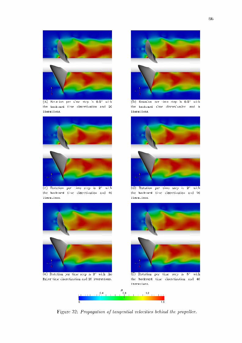
66

(a) Rotation per time step is 0.5◦ with

the backward time discretization and 20

iterations.

(b) Rotation per time step is 0.5◦ with

the backward time discretization and 5

iterations.

(c) Rotation per time step is 2◦ with

the backward time discretization and 40

iterations.

(d) Rotation per time step is 2◦ with

the backward time discretization and 20

iterations.

(e) Rotation per time step is 2◦ with the

Euler time discretization and 20 iterations.

(f) Rotation per time step is 5◦ with

the backward time discretization and 40

iterations.

Figure 32: Propagation of tangential velocities behind the propeller.

67

7 CRP Computation

All computational methods, that were chosen for the computations in this work,have been applied on the open-water case. The computational set-up has beenchosen, �xed and tested, and knowledge has been gained on how to use the relevantmethods. In this chapter, the methods are applied on the more complicated casethat has a thruster unit with two pushing propellers. Measurements have beenconducted with the same set-up in a towing tank as discussed in Chapter 1 [30].

The modelled geometry is shown in Figure 33. The yellow surfaces (outer walls,hub and shaft) are modelled as symmetry planes which e�ectively means that noth-ing can �ow through them and no friction is accounted for. Propeller blades arehandled in the same way as in the open-water case and the thruster surface is mod-elled as a wall. The thruster is divided in two parts. The lower part is submergedin water in the experimental set-up and the upper part is above the water line. Thecomputational domain spans approximately six propeller diameters upstream and�ve diameters downstream of the front propeller. There are ten diameters free spaceto both sides and downwards from the propeller axis and the space between the twopropellers is a quarter of the propeller diameter.

There are two propeller domains and a surrounding region in the computationalmesh that have all been meshed separately and afterwards merged together. Thesurfaces with discontinuities are illustrated in the lowest sub�gure of Figure 33. Theboundaries of the front propeller mesh are colored in turquoise and the boundariesof the aft propeller mesh in blue consistently with the propeller blades in othersub�gures. Between the two propeller meshes, there is yet another meshing interface(grey in the lowest sub�gure) where both sides move in the time-dependent case andwhere the MRF source changes direction in the steady-state computation.

The upstream side of the front propeller mesh is perpendicular to the incom-ing �ow direction (z-axis) and both outer boundaries are cylindrical surfaces. Theboundary between the two propeller meshes is divided in three parts. There is onepart perpendicular to the z-axis beginning from the hub and one limiting to thecylindrical outer boundaries. Between them, there is an axisymmetric surface thatconnects the other two parts. The reason for dividing the surface is to bring themesh interface su�ciently far from both propellers. Since the propeller tips are benttowards the downstream direction, a straight surface would unavoidably be close toeither one or both of the propellers. The downstream side boundary of the aft pro-peller mesh is a single axisymmetric surface that begins from the end of the hub andis tilted towards the downstream direction in order to avoid having the boundarytoo close to the aft propeller near the propeller tip.

The mesh has a total of 11.8 Mio. cells which is the largest number of cells thatcan be computed with the 16GB of RAM available in the workstation that was usedfor most of the computations. The propellers are meshed in exactly the same way asthe propeller in the open-water case. The blade surfaces are divided and the surfacemesh density is de�ned identically. Furthermore, the volume mesh in the surfacenormal direction is also similar to the mesh in the open-water case. Referring to theresults in the previous chapters, such a mesh around the propellers is not expected

68

to cause any considerable errors into the solution. The main parameters of thepropellers are approximately as given in Table 5.

Table 5: Main dimensions of the propellers.

Front propeller Aft propellerD [mm] 213 203Dhub [mm] 62 48

Number of blades 4 5

(a) Overall view of the modelled geometry.

(b) Closer view of the thruster unit.

(c) Propeller mesh boundaries (mesh discontinu-ities).

Figure 33: Geometry in the CRP case.

69

7.1 Results

As opposed to the open-water case, the CRP case is truly time-dependent whichis also seen in the global forces. No results were obtained with the MRF and itwas concluded that steady-state computations with multiple propellers are, if notimpossible, clearly involved with di�culties.

With the time-accurate code, thrust and torque coe�cients computed with theEuler time discretization, 2◦ of propeller rotation per time step and 35 inner iter-ations are shown in Figure 34. The contribution of each blade is shown separatelywith di�erent colors and the total value of the propeller is illustrated in black. Thetotal contribution varies in time at the frequency of a single blade of the front pro-peller passing the thruster unit. In the contributions of a single blade (colored linesin Figure 34), an additional frequency of the front propeller blade passing an aftpropeller blade is observed.

(a) Thrust coe�cient, KT on the front pro-peller.

(b) Torque coe�cient, KQ on the front pro-peller.

(c) Thrust coe�cient, KT on the aft pro-peller.

(d) Torque coe�cient, KQ on the aft pro-peller.

Figure 34: Thrust and torque coe�cients of the front and aft propellers of the CRPunit. Rotation per time step is 2◦ with the Euler time discretization and 35 iterations.

70

The force coe�cients computed with a 0.5◦ propeller rotation per time step aregiven in Figure 35. Additional variation of the coe�cients can be observed at theaft propeller. The shorter time step seems to reproduce more details about theinteraction between the propellers than the longer time step which is in line withthe discussion in the open-water case. The change in average values was, however,in the order of only half a percent.

(a) Thrust coe�cient, KT on the front pro-peller.

(b) Torque coe�cient, KQ on the front pro-peller.

(c) Thrust coe�cient, KT on the aft pro-peller.

(d) Torque coe�cient, KQ on the aft pro-peller.

Figure 35: Thrust and torque coe�cients of the front and aft propellers of the CRPunit. Rotation per time step is 0.5◦ with the Euler time discretization and 17 itera-tions.

The average levels of the force coe�cients are given in Table 6. The values aregiven in relative di�erences to the measured values in percent. The thrust on thefront propeller is overpredicted in both cases as is the torque on the aft propeller.The front propeller torque and the aft propeller thrust are underpredicted by two -three percent. The errors are considerably larger than those observed in the open-water case.

The results show that the time discretization with the parameters used clearlya�ects the solution. It does, however, not explain the whole deviation from themeasured values. Despite �nding the backward scheme bene�cial compared to the

71

Euler scheme, all the CRP results presented here are computed with the Eulerscheme. The reason for this is the larger memory requirements of the backwardscheme.

Table 6: Comparison of the aft and the front propeller force coe�cients to the mea-sured values. Results are given in relative di�erences to measured values in percent.

KT , fore KQ, fore KT , aft KQ, aft2◦/∆t, 16 iterations 5.2 -3.6 -2.5 8.22◦/∆t, 35 iterations 6.9 -2.3 -3.1 7.6

0.5◦/∆t, 17 iterations 7.4 -2.2 -2.3 8.0

The y+ values illustrated in Figure 36 reveal one source of uncertainty. Thefront propeller mesh yields to y+ values of greater than four in large areas of theblades. In the open-water case, the y+ values were smaller than 2 in most parts andthere was still a dependence on the grid in that case. There are also areas with highy+ values on the thruster which may a�ect the boundary layer development on thethruster and thus the thruster wake, too.

Figure 37 shows the velocity magnitude on a plane located behind the thruster.The velocity �eld clearly shows that the mesh between the thruster and the frontpropeller is too coarse. The non-conformal boundary between the surrounding partand the propeller meshes is clearly visible which is re�ected in the results. Since thein�ow to the front propeller is incorrect, it is di�cult to evaluate the correctness ofthe force prediction on either of the propellers.

Figure 36: y+ values.

72

(a) No mesh visible.

(b) Mesh visible.

Figure 37: Velocity �eld behind the thruster unit. The mesh boundary is clearly seendue to too coarse a mesh.

73

8 Conclusions and Discussion

Computational methods available in OpenFOAM were tested by applying them on theanalysis of marine propellers. The methods included the Moving Reference Frame(MRF) used to reduce the analysis of a rotating propeller into a steady-state problem.Furthermore, time-accurate computations were conducted using moving meshes andan iterative solution process inside each time step.

All methods were found to work well when applied on the analysis of a singlepropeller in open-water conditions. The �nal computational set-up is stable andpredicts propeller forces within approximately two percent of the measured valuesat moderate values of advance coe�cient. The methods have not been tested inbollard pull conditions.

When applied on a case with two propellers and a thruster unit in front of them,no steady-state results could be obtained. Even with the time-accurate code, forceprediction was no longer as good as in the case of a single propeller in open-waterconditions. There are several possible reasons for this. As discussed in Chapter7, the mesh was found to be too coarse both on the front propeller and in thespace between the front propeller and the thruster. With the current set-up andmesh, forces were predicted within eight percent of the measured values. Accordingto the literature review in Chapter 1, an accuracy of approximately �ve percentcould be expected in CRP computations in open-water conditions and additionaluncertainties are caused by the propellers operating in the thruster wake. In thisrespect, the results are acceptable but, since it was shown that the prediction ofthe thruster wake clearly poses uncertainties due to a coarse grid in this study, theevaluation of the reliablility of the code requires further studies.

The simulation must be continued with a re�ned mesh in order to reach reli-able estimates on the best possible accuracy of the computational method. It canbe stated here that such computations were made later and the e�ect of the griddiscontinuities on the results was solved. Further results will not be given in thiswork. In order to make further studies, a su�cient amount of computer resourcesshould be available. Most of the computations presented here were conducted witha workstation with six cores and 16GB of RAM. For further studies, the amountof RAM needs to be increased in order to allow the use of denser meshes and moreaccurate time discretizations. Doubling the RAM to 32GB would enable much moreaccurate studies. Furthermore, the number of cores should be increased. Adoptinga workstation with 16 cores would probably decrease the computation time even if�ner meshes were used. That would enable tests with a reasonable response timewhich is essential for e�cient working. The most demanding computations in thisstudy were conducted with 128 cores at CSC - IT Center for Science, that can pro-vide su�cient computer capacity. A more extensive use of the capacity o�ered bythem would provide a good basis for e�cient further studies.

An interesting path for additional studies is the evaluation of ways to reduce thecost of the computations. In this study, no wall functions were applied to reducethe number of cells near solid structures, since the main focus was on the evaluationof the other methods. Since the methods have now been found to work reliably, the

74

introduction of wall functions is an obvious topic for further studies. Even withoutthe wall functions, it could be expected that also multi-propeller applications canbe analysed in a feasible way with OpenFOAM. With the help of a few workstations,comparisons can be conducted in the time span of some weeks. Keeping in mind thepossibility of clusters and the advances in the computer technology, the durationof the computations does not seem to be a problem. The lack of licence costs inOpenFOAM further contributes to its feasibility. All in all, it seems probable that, afterthe proposed further studies, OpenFOAM will provide a reliable tool for the analysisof multi-propeller marine applications in R&D purposes.

75

References

[1] Lewis, E., Principles of Naval Architecture Volume II Resistance, Propulsionand Vibration. New Jersey, NJ: The Society of Naval Architects and MarineEngineers, 1988.

[2] Katz, J. and Plotkin, A., Low-Speed Aerodynamics. Cambridge: CambridgeUniversity Press, 2nd ed., 2001. ISBN 0�521�66219�2.

[3] OpenFOAM. http://www.openfoam.org.

[4] Carlton, J., Marine Propellers and Propulsion. Elsevier Ltd.

[5] Sanchez-Caja, A., Sipilä, T., and Pylkkänen, J., �Simulation of Viscous Flowaround a Ducted Propeller with Rudder Using Di�erent RANS-Based Ap-proaches,� in First International Symposium on Marine Propulsion, 2009.

[6] Ansys Inc., Canonsburg, PA 15317, USA, ANSYS FLUENT 13.0 User's Guide,2010.

[7] Guo, C., Ma, N., and Yang, C., �Numerical Simulation of a Podded Propulsorin Viscous Flow,� Journal of Hydrodynamics, Vol. 21, No. 1, 2009, pp. 71�76.

[8] Sanchez-Caja, A., Rautaheimo, P., Salminen, E., and Siikonen, T., �Compu-tation of the Incompressible Viscous Flow around a Tractor Thruster Usinga Sliding-Mesh Technique,� in Seventh International Conference on NumericalShip Hydrodynamics, July 1999.

[9] Wang, Z. and Xiong, Y., �E�ect of Time Step Size and Turbulence Model onthe Open Water Hydrodynamic Performance Prediction of Contra-RotatingPropellers,� China Ocean Eng., Vol. 27, No. 2, 2013, pp. 193�204.

[10] Feng, X., Lu, C., and Wu, Q., �Numerical Researches on interaction betweenPropellers in Uniform Flow,� Journal of Hydrodynamics, Vol. 24, No. 5, 2012,pp. 675�683.

[11] Dhinesh, G., Murali, K., and Subramanian, V., �Estimation of hull-propellerinteraction of a self-propelling model hull using RANSE solver,� Ships andO�shore Structures, Vol. 5, No. 2, 2010, pp. 125�139.

[12] Xia, L., Lundberg, J., and Bensow, R., �Performance Prediction of a NozzlePropeller,� in 29th Symposium on Naval Hydrodynamics, (Gothenburg).

[13] SVA, http://www.svapotsdam.de/towingtank.html, SVA website, Accessed2/17/2014.

[14] Farrell, P. E. and Maddison, J. R., �Conservative interpolation between volumemeshes by local Galerkin projection,� Comput. Methods Appl. Mech Engrg,Vol. 200, 2011, pp. 89�100.

76

[15] White, F. M., Viscous �uid �ow. Singapore: McGraw-Hill Book Co., 3nd ed.,2006. ISBN 0�07�124493�X.

[16] Holmes, D. and Tong, S., �A Three-Dimensional Euler Solver for Turbomachin-ery Blade Rows,� J. of Engineering and Gas Turbines and Power, Vol. 107,April 1985.

[17] Siikonen, T. and Pan, H., �Application of Roe's Method for the Simulation ofViscous Flow in Turbomachinery,� in Proceedings of the First European Compu-tational Fluid Dynamics Conference, (Brussels), pp. 635�641, Elsevier SciencePublishers B.V., Sept. 1992.

[18] Mans�eld, M. and O'Sullivan, C., Understanding Physics. Chichester: JohnWiley & Sons Ltd, 2006. ISBN10 0�470�06529�X.

[19] See the MRF development.http://openfoamwiki.net/index.php/See_the_MRF_development, 2013.

[20] Ferziger, J. and Peri¢, M., Computational methods for �uid dynamics. Berlin:Springer-Verlag, 3rd ed., 2002. ISBN 3�540�42074�6.

[21] Wilcox, D., Turbulence modeling for CFD. La Canada: DCW Industries, Inc.,1993. ISBN 0�9636051�0�0.

[22] Hellsten, A., �Some improvements in Menter's k − ω SST turbulence model,�in 29th AIAA Fluid Dynamics Conference, (Albuquerque, New Mexico, USA),AIAA paper 98�2554, 1998.

[23] OpenFOAM Foundation, OpenFOAM Programmer's Guide, version 2.2.0.

[24] Hirsch, C., Computational Methods for Inviscid and Viscous Flows, Vol. 2 ofNumerical Computation of Internal and External Flows. Chichester: John Wi-ley & Sons Ltd, 1990. ISBN 0�471�92351�6.

[25] Patankar, S., Numerical Heat Transfer and Fluid Flow. Washington, D.C:Hemisphere, 1980.

[26] Issa, R. I., �Solution of the Implicitly Discretised Fluid Flow Equations byOperator-Splitting,� Journal of Computational Physics, Vol. 62, No. 11, 1986,pp. 40�65.

[27] Balkmann, U., Heinke, H.-J., and Lübke, L., �Potsdam Propeller Test Case(PPTC), Test Case Description,� in Second International Symposium on MarinePropulsors.

[28] �Uncertainty Analysis in CFD, Veri�cation and Validation, Methodology andProcedures, 7.5−03−01−01,� International Towing Tank Conference (ITTC),2005.

77

[29] Eça, L. and Hoekstra, M., �A procedure for the estimation of the numericaluncertainty of CFD calculations based on grid re�nement studies,� Journal ofComputational Physics, Vol. 262, 2014, pp. 104�130.

[30] �Comparative Open Water and Cavitation Tests with Three Thrusters with CRPropellers,� SVAtech GmbH, Potsdam, 2012.