Embed Size (px)
Citation preview

Note: Turbidity Date: January 2018
1
www.leovanrijn-sediment.com
TURBIDITY DUE TO DREDGING AND DUMPING OF SEDIMENTS
by L.C. van Rijn, www.leovanrijn-sediment.com Content 1. Introduction 2. Dredging methods 3. Turbidity caused by dredging 3.1 General aspects 3.2 Turbidity values measured at field dredging sites 3.3 Measures reducing turbidity during dredging 3.4 Summary 3.5 Examples of predicted turbidity values at dredging sites 4. Turbidity at dumping sites 4.1 Dumping/disposal sites 4.2 Dumping processes in open water 4.3 Turbidity measured at field dumping sites 4.4 Examples of predicted turbidity values at dumping sites 5 Numerical simulation of dispersion processes 5.1 Theory of diffusion/dispersion/dilution processes 5.2 Settling and dispersion in uniform flow with and without lateral mixing 5.3 Dispersion by three -dimensional models 6. References
Note: Turbidity Date: January 2018
2
www.leovanrijn-sediment.com
1. Introduction Dredging of sediments deposited in harbour basins and approach channels is known as maintenance dredging and is a basic element of the economic performance of many ports. Usually, the dredged materials
consist of clay, silt and sand particles/flocs. The fraction with particles < 64 m is known as mud, the fraction
between 64 m and 2000 m (2 mm) is known as sand.
The mud fraction < 64 m can be subdivided in:
• fraction < 4 m; colloidal fraction (remaining in suspension in all conditions);
• fraction < 4-8 m; settling velocity 0.03 mm/s (flocculation limit 0.25 mm/s);
• fraction 8-16 m; settling velocity 0.12 mm/s; (flocculation limit 0.25 mm/s);
• fraction 16-32 m; settling velocity 0.45 mm/s;
• fraction 32-64 m; settling velocity 1.8 mm/s. The three essential elements of dredging are: excavation, transport and disposal. Often, the most critical elements are the excavation and the disposal (dumping) of sediments at the disposal site due to environmental pollution problems. In many cases the dredged material has to be dumped in the outer estuary or at open sea. Dumping in rivers and inner estuaries is most often not allowed if the dredged material is polluted. Efficient management of dredging works requires:
• detailed and regular monitoring of the area considered;
• sufficient knowledge of the sediment transport processes in the area considered;
• sufficient knowledge of dredging and disposal methods;
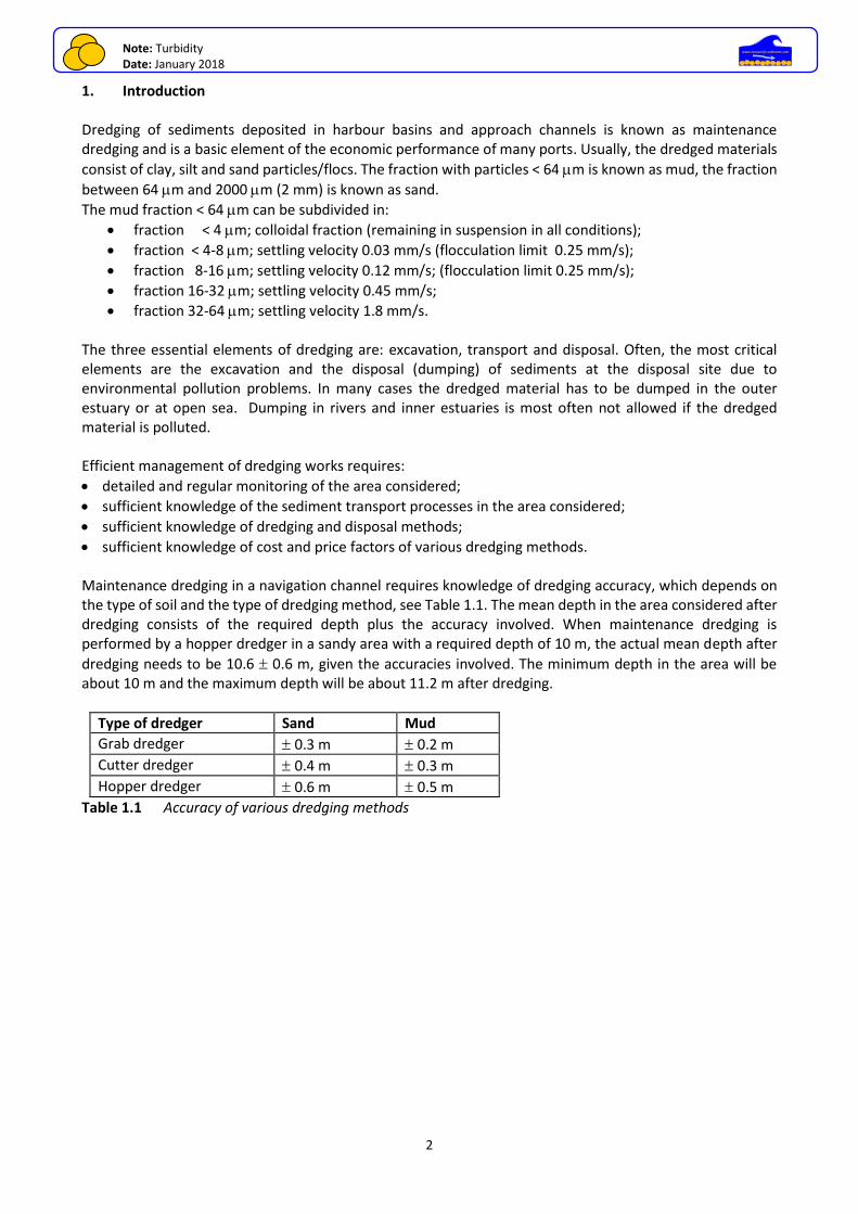
• sufficient knowledge of cost and price factors of various dredging methods. Maintenance dredging in a navigation channel requires knowledge of dredging accuracy, which depends on the type of soil and the type of dredging method, see Table 1.1. The mean depth in the area considered after dredging consists of the required depth plus the accuracy involved. When maintenance dredging is performed by a hopper dredger in a sandy area with a required depth of 10 m, the actual mean depth after
dredging needs to be 10.6 0.6 m, given the accuracies involved. The minimum depth in the area will be about 10 m and the maximum depth will be about 11.2 m after dredging.
Type of dredger Sand Mud
Grab dredger 0.3 m 0.2 m
Cutter dredger 0.4 m 0.3 m
Hopper dredger 0.6 m 0.5 m
Table 1.1 Accuracy of various dredging methods

Note: Turbidity Date: January 2018
3
www.leovanrijn-sediment.com
2. Dredging methods Each type of dredger has its own typical characteristics such as:
• sensitivity to waves and currents (operational conditions);
• minimum water depth required for excavation (dredging) and sailing;
• minimum horizontal channel dimensions required for manoeuvering;
• type of soils that can be dredged;
• production in relation to soil composition;
• vertical accuracy of dredged bed profile. The following three main types of dredging methods are available:
• Cutter dredging (hydraulic); - positioned by anchors (hindrance to ships); - sensitive to waves and currents; - connected to floating pipe line (removal of dredged materials); - large range of soils (soft to consolidated, rocky soils); - large production range (upto 10,000 m3/hour); 10% to 20% solids (by weight) in slurry; - reasonably smooth bed profile after dredging; - wide suction mouth can be used to remove a wide, but thin layer (dustpan dredger);
• Trailing-suction hopper dredging (hydraulic); - self sailing with suction pipes and draghead suspended from cables (midships alongside); - sediment is pumped into hopper and excess water is ultimately forced to flow overboard; - no hindrance to other ships (no floating pipeline); - not very sensitive to waves and currents; - minimum water depth required for dredging and sailing (approx. 7 m); - suitable for relatively soft unconsolidated soils; - very suitable for large channel maintenance projects; - large production range (up to 10,000 m3/hour); - unloading through pipeline pumping; by rainbowing or by bottom-doors; - rough bed profile after dredging; - environmental problems due to overflow;
• Grab dredging by crane/backhoe (mechanical); - dredging from a fixed platform (hindrance); - able to work close to structures (piers, quays); - not sensitive to waves and currents; - closed clamshell bucket for minimum turbidity levels; - removal of dredged material by barges for off-site transport; - small production range (500 m3/hour); - large range of soils (soft clay to soft rock); - smooth bed profile after dredging.
During dredging and dumping activities, mud is most often released in the system as spill (side effect). Two types of mud spill sources can be distinguished (see also Table 2.1):
• single point-spill event (< 1 hour; spill area of 10x10 m2) generating a mud cloud; the mud cloud is carried downstream by the current and the mud concentration decreases due to settling and mixing (vertical , longitudinal and lateral); Examples: mud overflow from a hopper dredger; mud dumping though bottom doors of barge
• (semi)continuous point-spill over a certain period (hours to days; spill area 10x10 m2); Examples: free fall spraying of sand-mud into the water (rainbowing ) to make land.
Note: Turbidity Date: January 2018
4
www.leovanrijn-sediment.com
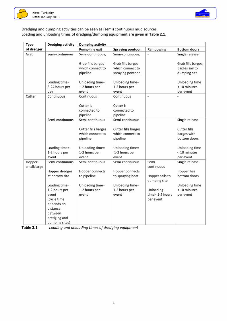
Dredging and dumping activities can be seen as (semi) continuous mud sources. Loading and unloading times of dredging/dumping equipment are given in Table 2.1.
Type of dredger
Dredging activity Dumping activity
Pump-line exit Spraying pontoon Rainbowing Bottom doors
Grab Semi-continuous Loading time= 8-24 hours per day
Semi-continuous; Grab fills barges which connect to pipeline Unloading time= 1-2 hours per event
Semi-continuous; Grab fills barges which connect to spraying pontoon Unloading time= 1-2 hours per event
- Single release Grab fills barges; Barges sail to dumping site Unloading time < 10 minutes per event
Cutter Continuous Continuous Cutter is connected to pipeline
Continuous Cutter is connected to pipeline
- -
Semi-continuous Loading time= 1-2 hours per event
Semi-continuous Cutter fills barges which connect to pipeline Unloading time= 1-2 hours per event
Semi-continuous Cutter fills barges which connect to pipeline Unloading time= 1-2 hours per event
- Single release Cutter fills barges with bottom doors Unloading time < 10 minutes per event
Hopper-small/large
Semi-continuous Hopper dredges at borrow site Loading time= 1-2 hours per event (cycle time depends on distance between dredging and dumping sites)
Semi-continuous Hopper connects to pipeline Unloading time= 1-2 hours per event
Semi-continuous Hopper connects to spraying boat Unloading time= 1-2 hours per event
Semi-continuous Hopper sails to dumping site Unloading time= 1-2 hours per event
Single release Hopper has bottom doors Unloading time < 10 minutes per event
Table 2.1 Loading and unloading times of dredging equipment
Note: Turbidity Date: January 2018
5
www.leovanrijn-sediment.com
3. Turbidity caused by dredging 3.1 General aspects The increase of suspended sediment concentrations due to the dredging process is generally expressed as a total suspended solids concentration (TSS in kg/m3; gr/l or in mg/l). TSS is a simple measure of the dry-weight mass of non-dissolved solids suspended per unit volume of water. TSS includes inorganic solids such as clay, silt, sand, etc. It may also include organic solids such as algae, zooplankton, and detritus, depending on the type of analysis method. When direct measurement of the quantity of suspended particulate matter present in water is needed, TSS mass determination in a laboratory is the most common method. Turbidity is a common standard method used to describe the cloudy or muddy appearance of water. Turbidity measurements have often been used for water quality studies because they are relatively quick and easy to perform in the field. The concept of turbidity involves optical properties of the water and is not a direct measure of the concentration of suspended sediments. Turbidity has been defined as an optical measurement of light that is scattered and absorbed. The standard unit of measurement for turbidity is the Nephelometric Turbidity Unit (NTU) measured with a nephelometer. NTUs are based on a standard
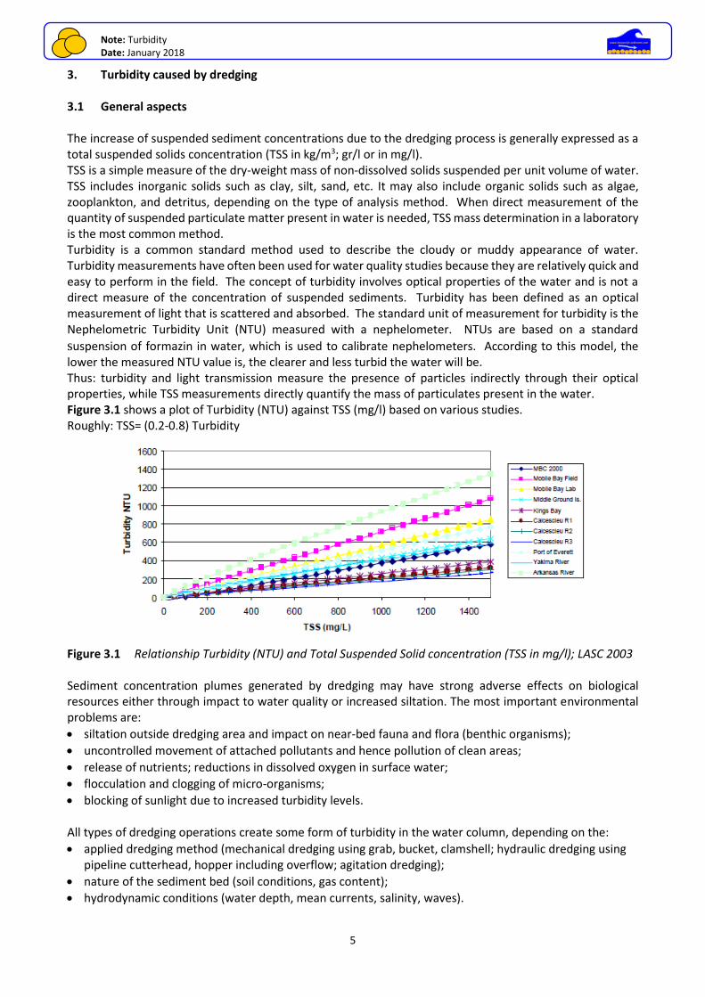
suspension of formazin in water, which is used to calibrate nephelometers. According to this model, the lower the measured NTU value is, the clearer and less turbid the water will be. Thus: turbidity and light transmission measure the presence of particles indirectly through their optical properties, while TSS measurements directly quantify the mass of particulates present in the water. Figure 3.1 shows a plot of Turbidity (NTU) against TSS (mg/l) based on various studies. Roughly: TSS= (0.2-0.8) Turbidity
Figure 3.1 Relationship Turbidity (NTU) and Total Suspended Solid concentration (TSS in mg/l); LASC 2003 Sediment concentration plumes generated by dredging may have strong adverse effects on biological resources either through impact to water quality or increased siltation. The most important environmental problems are:
• siltation outside dredging area and impact on near-bed fauna and flora (benthic organisms);
• uncontrolled movement of attached pollutants and hence pollution of clean areas;
• release of nutrients; reductions in dissolved oxygen in surface water;
• flocculation and clogging of micro-organisms;
• blocking of sunlight due to increased turbidity levels. All types of dredging operations create some form of turbidity in the water column, depending on the:
• applied dredging method (mechanical dredging using grab, bucket, clamshell; hydraulic dredging using pipeline cutterhead, hopper including overflow; agitation dredging);
• nature of the sediment bed (soil conditions, gas content);
• hydrodynamic conditions (water depth, mean currents, salinity, waves).
Note: Turbidity Date: January 2018
6
www.leovanrijn-sediment.com
Turbidity during dredging activities is caused by the:
• actual dredging/excavation process at the sediment bed (resuspension effect), including gas releases from disturbed bed;
• spillage during vertical transportation from bed to vessel or barge; - grab dredger and bucket dredger: sediments washed off during vertical movements; impact on bed, losses during emptying in barge; - hopper dredger: movement of suction pipes through bed, return flow under vessel during sailing, jet flow due to propeller of vessel, emptying of suction pipes after blockings (flow reversal in pipe), overflow during filling process (pumping continues after hopper is full in order to displace the water and increase the material density in the hopper, excess sediment-laden water overflows and re-enters the water column);
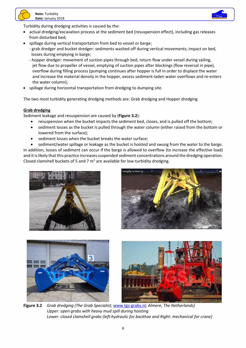
• spillage during horizontal transportation from dredging to dumping site. The two most turbidity generating dredging methods are: Grab dredging and Hopper dredging Grab dredging Sediment leakage and resuspension are caused by (Figure 3.2):
• resuspension when the bucket impacts the sediment bed, closes, and is pulled off the bottom;
• sediment losses as the bucket is pulled through the water column (either raised from the bottom or lowered from the surface);
• sediment losses when the bucket breaks the water surface;
• sediment/water spillage or leakage as the bucket is hoisted and swung from the water to the barge. In addition, losses of sediment can occur if the barge is allowed to overflow (to increase the effective load) and it is likely that this practice increases suspended sediment concentrations around the dredging operation. Closed clamshell buckets of 5 and 7 m3 are available for low-turbidity dredging. Figure 3.2 Grab dredging (The Grab Specialist; www.tgs-grabs.nl; Almere, The Netherlands) Upper: open grabs with heavy mud spill during hoisting Lower: closed clamshell grabs (left:hydraulic for backhoe and Right: mechanical for crane)
Note: Turbidity Date: January 2018
7
www.leovanrijn-sediment.com
Hopper dredging Basically, the loading process consists of three phases (Van Rhee, 2002):
• filling phase to overflow level; three layers are present in the hopper: a lower layer of settled sand, a sediment-water mixture and a top layer of clear water;
• overflow phase (5 to 15 min); the hopper is filled with sand and the excess water is forced out of the hopper by overflow through a pipe system; a high-concentration density current is present above the bed gradually reducing in time; a low-concentration top layer is present near the water surface flowing in horizontal direction to the overflow system;
• final phase; high-concentration layer reaches the water surface and the overflow losses of sediment increase considerably; the maximum sediment concentrations in the overflow pipeline may be as large as 30% by volume when the hopper approaches its capacity .
In fine sandy conditions, the total overflow generally is of the order of 5% to 10%. In muddy conditions, the overflow can reach values up to 30% of the total volume of sediment pumped into the hopper and may cause significant environmental problems. Van Rhee (2002) performed large-scale laboratory tests (fine sand of 0.105 mm and 0.14 mm) of the hopper filling process and the associated overflow processes. The maximum overflow loss of sediment was about 40% in the tests with fine sand of 0.115 mm. A field hopper test at the sandy Dutch shoreface (Hopper Cornelia of Boskalis Westminster Dredging: B=11.5 m, L=52 m, Q=6 m3/s, d50=0.24 mm) showed an overflow loss of sand of about 8%. Van Parys et al. (2001) compared various techniques to reduce the turbidity during hopper dredging operations in the outer Port of Zeebrugge (Belgium). The turbidity levels were reduced by a factor 5 in case of dredging without overflow. 3.2 Turbidity values measured at field dredging sites Stuber (1976) presents data of turbidity studies during agitation dredging works near wharves, slips and docks (using drag beams behind tugs) in the Savannah River channel in the USA. The slips and wharves (siltation areas of 100x300 m2; water depths of about 10 m) are located adjacent to the main river channel and experience siltation rates in the range of 0.2 to 1 m per month. The tidal range varies in the range of 1.5 to 3 m; the peak tidal currents in the middle of the channel are in the range of 1 to 1.5 m/s. The background concentrations are in the range of 500 mg/l (near bed) to 50 mg/l (near surface). Agitation dredging is performed during ebb tidal flow. Suspended solids were measured at sampling control stations located at about 100 to 300 m downcurrent from the dredging sites and at a slightly greater distance from the bank than the centerline of the dredging area. Samples were taken at the water surface and at depths of about 4.5 m and 9 m from the water surface. The background concentrations varied in the range of 20 to 100 mg/l at most sites. The maximum silt concentrations in the downcurrent control stations varied in the range of 100 to 200 mg/l at a depth of 4.5 m and in the range of 200 to 400 mg/l near the bed (at depth of 9 m). The largest increase observed was from a background value of 30 mg/l to 300 mg/l during dredging (factor 10). Sosnowski (1984) studied the sediment resuspension near grab dredging works in the New Thames River and Eastern Long Island Sound (USA). The tidal range is about 1 m; the tidal currents are in the range of 0.5 to 0.8 m/s in the Thames River and in the range of 1.3 to 2 m/s in the Sound. The dredging operation consisted of a barge-mounted crane using an open clamshell bucket. Samples were taken at three depths (surface, mid-depth and near-bottom) in the dredge plume at 30 to 300 m downstream from the dredging site. Background concentrations were taken about 100 m upstream of the dredging site. Near the bottom the sediment concentrations were in the range of 100 to 1000 mg/l within 50 m from the dredging site. At a distance of about 300 m the near-bottom sediment concentrations were back to the background values of about 10 to 20 mg/l. Near the water surface the sediment concentrations were in the range of 10 to 100 mg/l within 50 m from the dredging site. At a distance of about 200 m the surface sediment concentrations were back to the background values of about 5 mg/l.
Note: Turbidity Date: January 2018
8
www.leovanrijn-sediment.com
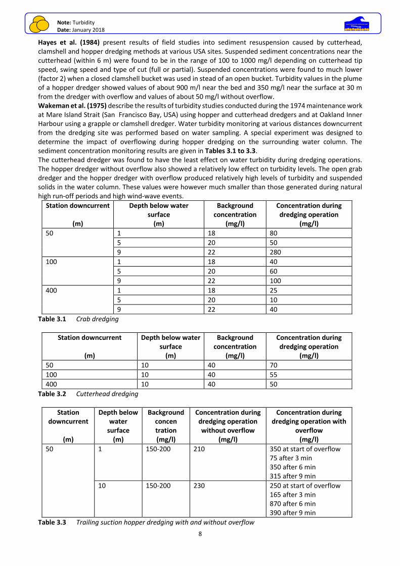
Hayes et al. (1984) present results of field studies into sediment resuspension caused by cutterhead, clamshell and hopper dredging methods at various USA sites. Suspended sediment concentrations near the cutterhead (within 6 m) were found to be in the range of 100 to 1000 mg/l depending on cutterhead tip speed, swing speed and type of cut (full or partial). Suspended concentrations were found to much lower (factor 2) when a closed clamshell bucket was used in stead of an open bucket. Turbidity values in the plume of a hopper dredger showed values of about 900 m/l near the bed and 350 mg/l near the surface at 30 m from the dredger with overflow and values of about 50 mg/l without overflow. Wakeman et al. (1975) describe the results of turbidity studies conducted during the 1974 maintenance work at Mare Island Strait (San Francisco Bay, USA) using hopper and cutterhead dredgers and at Oakland Inner Harbour using a grapple or clamshell dredger. Water turbidity monitoring at various distances downcurrent from the dredging site was performed based on water sampling. A special experiment was designed to determine the impact of overflowing during hopper dredging on the surrounding water column. The sediment concentration monitoring results are given in Tables 3.1 to 3.3. The cutterhead dredger was found to have the least effect on water turbidity during dredging operations. The hopper dredger without overflow also showed a relatively low effect on turbidity levels. The open grab dredger and the hopper dredger with overflow produced relatively high levels of turbidity and suspended solids in the water column. These values were however much smaller than those generated during natural high run-off periods and high wind-wave events.
Station downcurrent
(m)
Depth below water surface
(m)
Background concentration
(mg/l)
Concentration during dredging operation
(mg/l)
50 1 18 80
5 20 50
9 22 280
100 1 18 40
5 20 60
9 22 100
400 1 18 25
5 20 10
9 22 40
Table 3.1 Crab dredging
Station downcurrent
(m)
Depth below water surface
(m)
Background concentration
(mg/l)
Concentration during dredging operation
(mg/l)
50 10 40 70
100 10 40 55
400 10 40 50
Table 3.2 Cutterhead dredging
Station downcurrent
(m)
Depth below water
surface (m)
Background concen tration (mg/l)
Concentration during dredging operation without overflow
(mg/l)
Concentration during dredging operation with
overflow (mg/l)
50 1 150-200 210 350 at start of overflow 75 after 3 min 350 after 6 min 315 after 9 min
10 150-200 230 250 at start of overflow 165 after 3 min 870 after 6 min 390 after 9 min
Table 3.3 Trailing suction hopper dredging with and without overflow
Note: Turbidity Date: January 2018
9
www.leovanrijn-sediment.com
Bernard (1978) synthesizes the results of eight research studies into sediment resuspension and turbidity levels near various dredging sites in the USA. Water-column turbidity generated by dredging operations is usually restricted to the vicinity of the operation and decreases rapidly with increasing distance from the operation. The results can be summarized, as follows:
• Grab (Clamshell): maximum concentrations of suspended solids within 50 to 100 m from the dredging site will be less than about 200 mg/l; the visible plume will be about 300 m long at the surface and approximately 500 m near the bottom; maximum concentrations will decrease rapidly to background values within 500 m;
• Cutter: the increase of suspended concentrations around cutterhead dredges is restricted to the immediate vicinity of the cutter, where concentrations may be as high as 10 gr/l within 3 m of the cutter; near-bottom levels of 100 to 200 mg/l may be found within a few hundred metres of the cutter;
• Hopper: during overflow operations, turbidity plumes with concentrations of 200 to 300 mg/l may extend behind the dredge for distances up to 1200 m; without overflow the concentrations are considerably smaller (factor 3 to 5); near-bottom concentrations of 1 to 2 gr/l are generated near the dragheads.
Turbidity levels around dredging operations can be reduced when necessary, but not without appreciable cost, by improving existing cutterhead dredging equipment techniques (large sets and very thick cuts should be avoided), using watertight buckets and eliminating hopper dredge overflow, or using a submerged overflow system. The dispersion of near-surface turbidity can be controlled, to a certain extent, by placing a silt curtain downstream or around certain types of dredging/disposal operations. Under quiescent current conditions (<0.1 m/s) turbidity levels in the water column outside the curtain may be reduced by as much as 80 to 90 percent. Silt curtains can not be used in conditions with currents larger than 0.5 m/s. Willoughby and Crabb (1983) studied the behaviour of dredge-generated sediment plumes in Moreton Bay, Australia. The data were collected during June and July 1982 in the overflow plume generated from a trailing suction hopper dredger during sand (0.25 mm) dredging at Middle Banks in the Bay area. Close to the dredge, the measured concentrations ranged between about 500 mg/l (near the bed) and 50 mg/l (near the surface). The background concentration were of the order of about 5 mg/l. The concentrations in the plume were found to be reduced to at or just above background levels within approximately one hour. About 90% of this reduction occurred within the first 20 minutes. Given the local current velocity of about 0.6 m/s, the major proportion of the dredge suspended material settled within about 600 to 700 m downcurrent from the dredge. Battisto and Friedrichs (2003) studied the suspended sediment plume characteristics during oyster shell dredging (on 22 August 2001; northeast of Hogg Island in the James River estuary, Virginia, USA) using ADCP, OBS and bottle samples. During strong tidal flow, the dredge plume was confined mainly to the bottom of the estuary channel with a width of about 200 m and an estimated maximum length of 5 km. At distances of 100 to 400 m downstream of the dredge, the plume was about 1 to 2 m thick with concentrations of 50 to 100 mg/l higher than the background values of about 100 mg/l. At distances of 700 m downstream of the dredge, the plume was about 3 to 4 m thick with concentrations of 30 to 50 mg/l higher than the background values (100 mg/l). Active dredging around slack water produced a spatially less extensive but higher concentration suspension in the immediate vicinity of the dredge. During slack after ebb, a plume of 8 m thick, 200 m wide and concentration of 100 mg/l was formed near the dredge before collapsing and spreading along the bottom of the main channel as a layer of 1.5 m thick, concentrations up to 150 to 200 mg/l and an estimated length of 500 m. This concentration pool was then advanced landward with the flood tide. When dredging was stopped at slack after flood, the plume outside the immediate vicinity of the dredge settled to below detection levels within an hour. Comparison of OBS and ADCP profiles showed good agreement. A typical ADCP transect across the dredge plume provides better visualization of the extent of the dredge plume than is possible with only OBS profiles.
Note: Turbidity Date: January 2018
10
www.leovanrijn-sediment.com
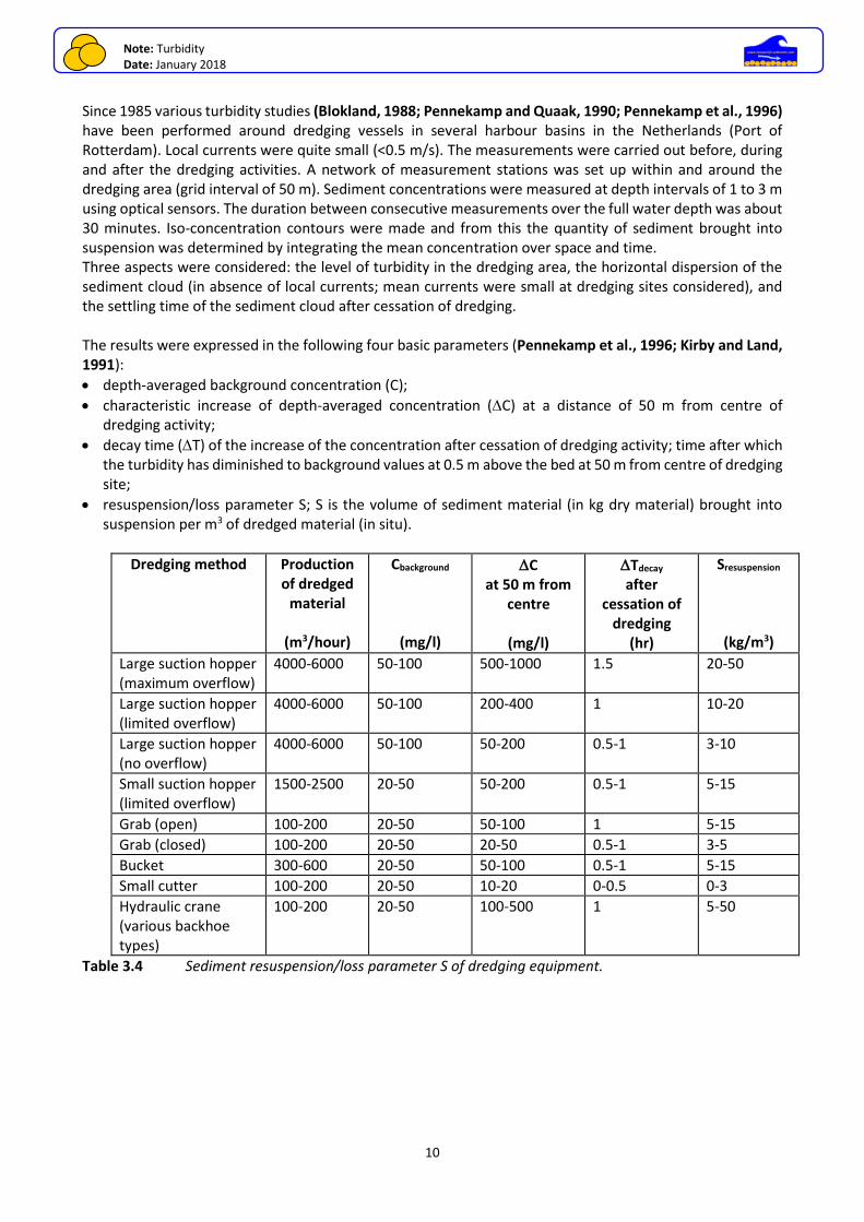
Since 1985 various turbidity studies (Blokland, 1988; Pennekamp and Quaak, 1990; Pennekamp et al., 1996) have been performed around dredging vessels in several harbour basins in the Netherlands (Port of Rotterdam). Local currents were quite small (<0.5 m/s). The measurements were carried out before, during and after the dredging activities. A network of measurement stations was set up within and around the dredging area (grid interval of 50 m). Sediment concentrations were measured at depth intervals of 1 to 3 m using optical sensors. The duration between consecutive measurements over the full water depth was about 30 minutes. Iso-concentration contours were made and from this the quantity of sediment brought into suspension was determined by integrating the mean concentration over space and time. Three aspects were considered: the level of turbidity in the dredging area, the horizontal dispersion of the sediment cloud (in absence of local currents; mean currents were small at dredging sites considered), and the settling time of the sediment cloud after cessation of dredging. The results were expressed in the following four basic parameters (Pennekamp et al., 1996; Kirby and Land, 1991):
• depth-averaged background concentration (C);
• characteristic increase of depth-averaged concentration (C) at a distance of 50 m from centre of dredging activity;
• decay time (T) of the increase of the concentration after cessation of dredging activity; time after which the turbidity has diminished to background values at 0.5 m above the bed at 50 m from centre of dredging site;
• resuspension/loss parameter S; S is the volume of sediment material (in kg dry material) brought into suspension per m3 of dredged material (in situ).
Dredging method Production of dredged
material
(m3/hour)
Cbackground
(mg/l)
C at 50 m from
centre
(mg/l)
Tdecay after
cessation of dredging
(hr)
Sresuspension
(kg/m3)
Large suction hopper (maximum overflow)
4000-6000 50-100 500-1000 1.5 20-50
Large suction hopper (limited overflow)
4000-6000 50-100 200-400 1 10-20
Large suction hopper (no overflow)
4000-6000 50-100 50-200 0.5-1 3-10
Small suction hopper (limited overflow)
1500-2500 20-50 50-200 0.5-1 5-15
Grab (open) 100-200 20-50 50-100 1 5-15
Grab (closed) 100-200 20-50 20-50 0.5-1 3-5
Bucket 300-600 20-50 50-100 0.5-1 5-15
Small cutter 100-200 20-50 10-20 0-0.5 0-3
Hydraulic crane (various backhoe types)
100-200 20-50 100-500 1 5-50
Table 3.4 Sediment resuspension/loss parameter S of dredging equipment.
Note: Turbidity Date: January 2018
11
www.leovanrijn-sediment.com
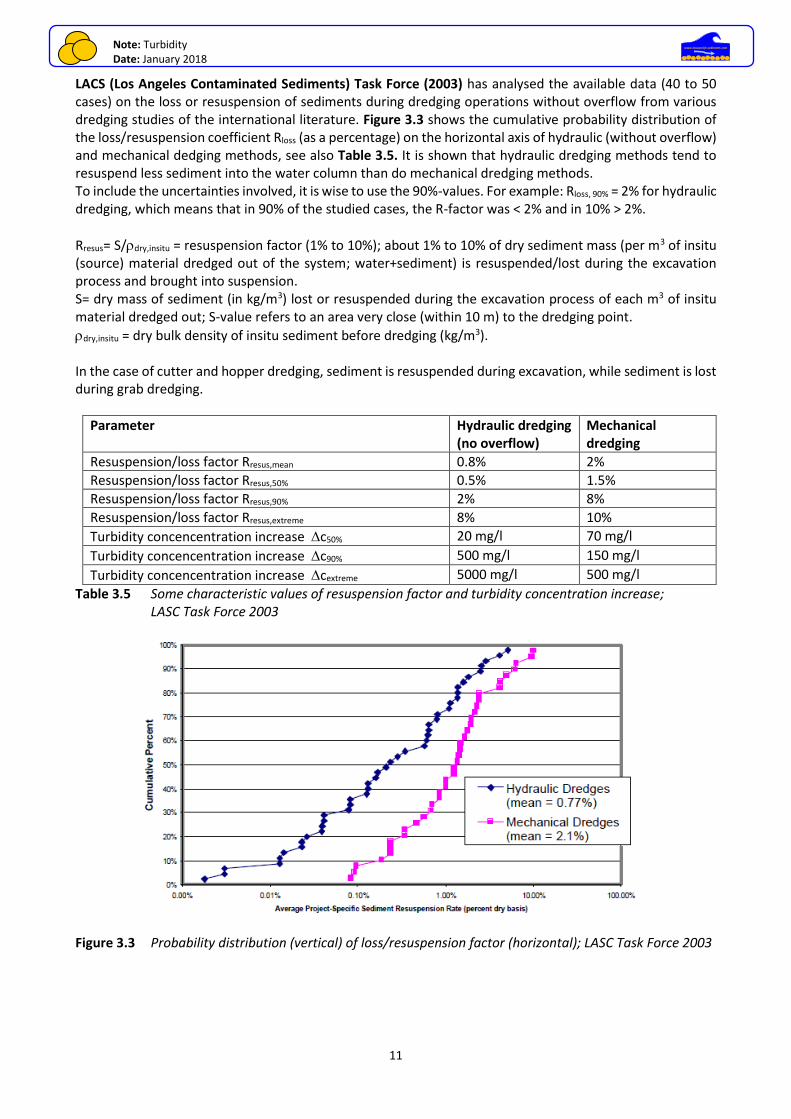
LACS (Los Angeles Contaminated Sediments) Task Force (2003) has analysed the available data (40 to 50 cases) on the loss or resuspension of sediments during dredging operations without overflow from various dredging studies of the international literature. Figure 3.3 shows the cumulative probability distribution of the loss/resuspension coefficient Rloss (as a percentage) on the horizontal axis of hydraulic (without overflow) and mechanical dedging methods, see also Table 3.5. It is shown that hydraulic dredging methods tend to resuspend less sediment into the water column than do mechanical dredging methods. To include the uncertainties involved, it is wise to use the 90%-values. For example: Rloss, 90% = 2% for hydraulic dredging, which means that in 90% of the studied cases, the R-factor was < 2% and in 10% > 2%.
Rresus= S/dry,insitu = resuspension factor (1% to 10%); about 1% to 10% of dry sediment mass (per m3 of insitu (source) material dredged out of the system; water+sediment) is resuspended/lost during the excavation process and brought into suspension. S= dry mass of sediment (in kg/m3) lost or resuspended during the excavation process of each m3 of insitu material dredged out; S-value refers to an area very close (within 10 m) to the dredging point.
dry,insitu = dry bulk density of insitu sediment before dredging (kg/m3). In the case of cutter and hopper dredging, sediment is resuspended during excavation, while sediment is lost during grab dredging.
Parameter Hydraulic dredging (no overflow)
Mechanical dredging
Resuspension/loss factor Rresus,mean 0.8% 2%
Resuspension/loss factor Rresus,50% 0.5% 1.5%
Resuspension/loss factor Rresus,90% 2% 8%
Resuspension/loss factor Rresus,extreme 8% 10%
Turbidity concencentration increase c50% 20 mg/l 70 mg/l
Turbidity concencentration increase c90% 500 mg/l 150 mg/l
Turbidity concencentration increase cextreme 5000 mg/l 500 mg/l
Table 3.5 Some characteristic values of resuspension factor and turbidity concentration increase; LASC Task Force 2003
Figure 3.3 Probability distribution (vertical) of loss/resuspension factor (horizontal); LASC Task Force 2003
Note: Turbidity Date: January 2018
12
www.leovanrijn-sediment.com
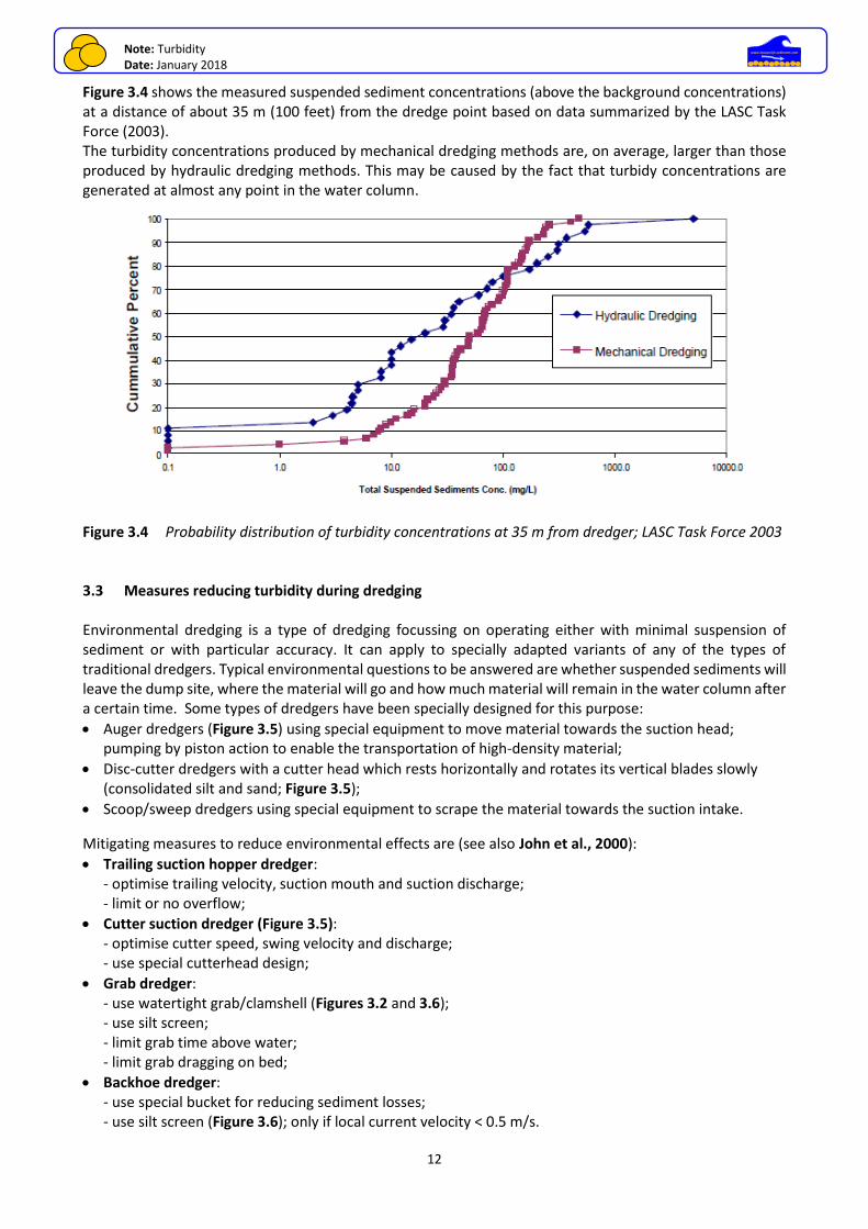
Figure 3.4 shows the measured suspended sediment concentrations (above the background concentrations) at a distance of about 35 m (100 feet) from the dredge point based on data summarized by the LASC Task Force (2003). The turbidity concentrations produced by mechanical dredging methods are, on average, larger than those produced by hydraulic dredging methods. This may be caused by the fact that turbidy concentrations are generated at almost any point in the water column.
Figure 3.4 Probability distribution of turbidity concentrations at 35 m from dredger; LASC Task Force 2003 3.3 Measures reducing turbidity during dredging Environmental dredging is a type of dredging focussing on operating either with minimal suspension of sediment or with particular accuracy. It can apply to specially adapted variants of any of the types of traditional dredgers. Typical environmental questions to be answered are whether suspended sediments will leave the dump site, where the material will go and how much material will remain in the water column after a certain time. Some types of dredgers have been specially designed for this purpose:
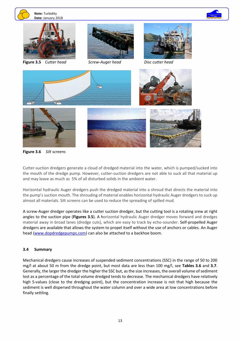
• Auger dredgers (Figure 3.5) using special equipment to move material towards the suction head; pumping by piston action to enable the transportation of high-density material;
• Disc-cutter dredgers with a cutter head which rests horizontally and rotates its vertical blades slowly (consolidated silt and sand; Figure 3.5);
• Scoop/sweep dredgers using special equipment to scrape the material towards the suction intake.
Mitigating measures to reduce environmental effects are (see also John et al., 2000):
• Trailing suction hopper dredger: - optimise trailing velocity, suction mouth and suction discharge; - limit or no overflow;
• Cutter suction dredger (Figure 3.5): - optimise cutter speed, swing velocity and discharge; - use special cutterhead design;
• Grab dredger: - use watertight grab/clamshell (Figures 3.2 and 3.6); - use silt screen; - limit grab time above water; - limit grab dragging on bed;
• Backhoe dredger: - use special bucket for reducing sediment losses; - use silt screen (Figure 3.6); only if local current velocity < 0.5 m/s.
Note: Turbidity Date: January 2018
13
www.leovanrijn-sediment.com
Figure 3.5 Cutter head Screw-Auger head Disc cutter head
Figure 3.6 Silt screens Cutter-suction dredgers generate a cloud of dredged material into the water, which is pumped/sucked into the mouth of the dredge pump. However, cutter-suction dredgers are not able to suck all that material up and may leave as much as 5% of all disturbed solids in the ambient water. Horizontal hydraulic Auger dredgers push the dredged material into a shroud that directs the material into the pump’s suction mouth. The shrouding of material enables horizontal hydraulic Auger dredgers to suck up almost all materials. Silt screens can be used to reduce the spreading of spilled mud. A screw-Auger dredger operates like a cutter suction dredger, but the cutting tool is a rotating srew at right angles to the suction pipe (Figures 3.5). A horizontal hydraulic Auger dredger moves forward and dredges material away in broad lanes (dredge cuts), which are easy to track by echo-sounder. Self-propelled Auger dredgers are available that allows the system to propel itself without the use of anchors or cables. An Auger head (www.dopdredgepumps.com) can also be attached to a backhoe boom. 3.4 Summary Mechanical dredgers cause increases of suspended sediment concentrations (SSC) in the range of 50 to 200 mg/l at about 50 m from the dredge point, but most data are less than 100 mg/l, see Tables 3.6 and 3.7. Generally, the larger the dredger the higher the SSC but, as the size increases, the overall volume of sediment lost as a percentage of the total volume dredged tends to decrease. The mechanical dredgers have relatively high S-values (close to the dredging point), but the concentration increase is not that high because the sediment is well dispersed throughout the water column and over a wide area at low concentrations before finally settling.
Note: Turbidity Date: January 2018
14
www.leovanrijn-sediment.com
Table 3.8 shows dilution factors based on measured data and theoretical dispersion studies (Section 5). In most cases, the SSC decay to the background values within 500 m, except for hopper dredging with overflow. Cutter suction dredgers produce SSC which are quite high near the cutterhead (about 1,000 to 10,000 mg/l), but are quite small away from the cutter. Trailing suction hopper dredgers can inject considerable quantities of fines into the water column when overflowing. SSC close behind the dredger can reach up to 500 mg/l at the water surface and as much as 5000 mg/l near the bed. If operating without overflow, very little sediment is brought into suspension (generally smaller than about 200 mg/l). The overflow mixture tends to descend towards the bed quite rapidly as a dense plume due to its relatively high density and high rate of delivery. Large suction hopper dredgers can produce just as much turbidity (in terms of S-values) as small Backhoe grab dredgers. The S-values do not depend greatly on production capacity. The study results from various field sites show that the turbidity concentrations:
• are greatest near the bottom;
• decrease rapidly with distance from the dredger; decrease is less rapid if currents are relatively large;
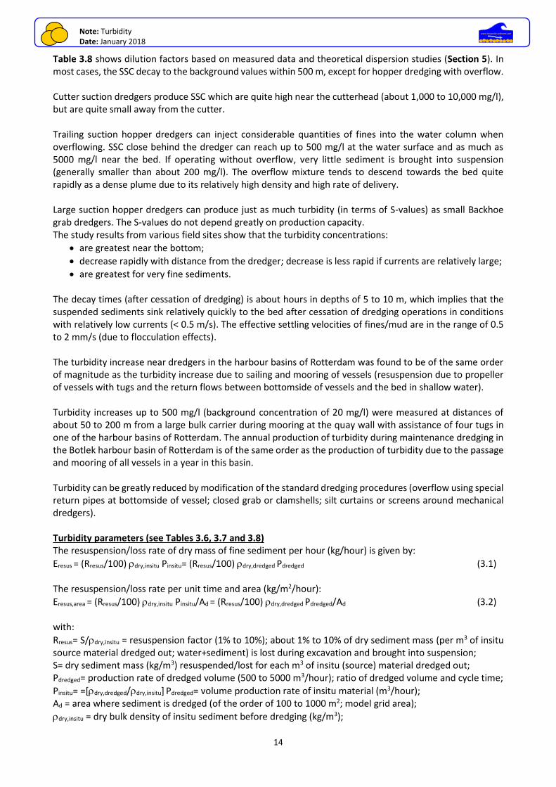
• are greatest for very fine sediments. The decay times (after cessation of dredging) is about hours in depths of 5 to 10 m, which implies that the suspended sediments sink relatively quickly to the bed after cessation of dredging operations in conditions with relatively low currents (< 0.5 m/s). The effective settling velocities of fines/mud are in the range of 0.5 to 2 mm/s (due to flocculation effects). The turbidity increase near dredgers in the harbour basins of Rotterdam was found to be of the same order of magnitude as the turbidity increase due to sailing and mooring of vessels (resuspension due to propeller of vessels with tugs and the return flows between bottomside of vessels and the bed in shallow water). Turbidity increases up to 500 mg/l (background concentration of 20 mg/l) were measured at distances of about 50 to 200 m from a large bulk carrier during mooring at the quay wall with assistance of four tugs in one of the harbour basins of Rotterdam. The annual production of turbidity during maintenance dredging in the Botlek harbour basin of Rotterdam is of the same order as the production of turbidity due to the passage and mooring of all vessels in a year in this basin. Turbidity can be greatly reduced by modification of the standard dredging procedures (overflow using special return pipes at bottomside of vessel; closed grab or clamshells; silt curtains or screens around mechanical dredgers). Turbidity parameters (see Tables 3.6, 3.7 and 3.8) The resuspension/loss rate of dry mass of fine sediment per hour (kg/hour) is given by:
Eresus = (Rresus/100) dry,insitu Pinsitu= (Rresus/100) dry,dredged Pdredged (3.1) The resuspension/loss rate per unit time and area (kg/m2/hour):
Eresus,area = (Rresus/100) dry,insitu Pinsitu/Ad = (Rresus/100) dry,dredged Pdredged/Ad (3.2) with:
Rresus= S/dry,insitu = resuspension factor (1% to 10%); about 1% to 10% of dry sediment mass (per m3 of insitu source material dredged out; water+sediment) is lost during excavation and brought into suspension; S= dry sediment mass (kg/m3) resuspended/lost for each m3 of insitu (source) material dredged out; Pdredged= production rate of dredged volume (500 to 5000 m3/hour); ratio of dredged volume and cycle time;
Pinsitu= =[dry,dredged/dry,insitu] Pdredged= volume production rate of insitu material (m3/hour); Ad = area where sediment is dredged (of the order of 100 to 1000 m2; model grid area);
dry,insitu = dry bulk density of insitu sediment before dredging (kg/m3);
Note: Turbidity Date: January 2018
15
www.leovanrijn-sediment.com
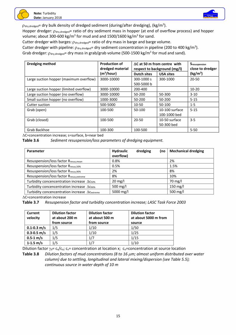
dry,dredged= dry bulk density of dredged sediment (during/after dredging), (kg/m3).
Hopper dredger: dry,dredged= ratio of dry sediment mass in hopper (at end of overflow process) and hopper volume; about 300-600 kg/m3 for mud and and 1500/1600 kg/m3 for sand.
Cutter dredger with barges: dry,dredged= ratio of dry mass in barge and barge volume.
Cutter dredger with pipeline: dry,dredged= dry sediment concentration in pipeline (200 to 400 kg/m3).
Grab dredger: dry,dredged= dry mass in grab/grab volume (500-1500 kg/m3 for mud and sand).
Dredging method Production of dredged material (m3/hour)
C at 50 m from centre with respect to background (mg/l)
Sresuspension
close to dredger (kg/m3) Dutch sites USA sites
Large suction hopper (maximum overflow) 3000-10000 300-1000 s 500-5000 b
300-1000 20-50
Large suction hopper (limited overflow) 3000-10000 200-400 10-20
Large suction hopper (no overflow) 3000-10000 50-200 50-300 3-10
Small suction hopper (no overflow) 1000-3000 50-200 50-200 5-15
Cutter suction 500-5000 10-50 50-100 1-5
Grab (open) 100-500 50-100 10-100 surface 100-1000 bed
5-15
Grab (closed) 100-500 20-50 10-50 surface 50-300 bed
3-5
Grab Backhoe 100-300 100-500 5-50
C=concentration increase; s=surface, b=near bed Table 3.6 Sediment resuspension/loss parameters of dredging equipment.
Parameter Hydraulic dredging (no overflow)
Mechanical dredging
Resuspension/loss factor Rresus,mean 0.8% 2%
Resuspension/loss factor Rresus,50% 0.5% 1.5%
Resuspension/loss factor Rresus,90% 2% 8%
Resuspension/loss factor Rresus,extreme 8% 10%
Turbidity concencentration increase c50% 20 mg/l 70 mg/l
Turbidity concencentration increase c90% 500 mg/l 150 mg/l
Turbidity concencentration increase cextreme 5000 mg/l 500 mg/l
C=concentration increase Table 3.7 Resuspension factor and turbidity concentration increase; LASC Task Force 2003
Current velocity
Dilution factor at about 200 m from source
Dilution factor at about 500 m from source
Dilution factor at about 5000 m from source
0.1-0.3 m/s 1/5 1/10 1/50
0.3-0.5 m/s 1/5 1/10 1/25
0.5-1 m/s 1/5 1/7 1/15
1-1.5 m/s 1/5 1/7 1/10
Dilution factor d= cx/co; cx= concentration at location x; co=concentration at source location
Table 3.8 Dilution factors of mud concentrations (8 to 16 m; almost uniform distributed over water column) due to settling, longitudinal and lateral mixing/dispersion (see Table 5.5);
continuous source in water depth of 10 m
Note: Turbidity Date: January 2018
16
www.leovanrijn-sediment.com
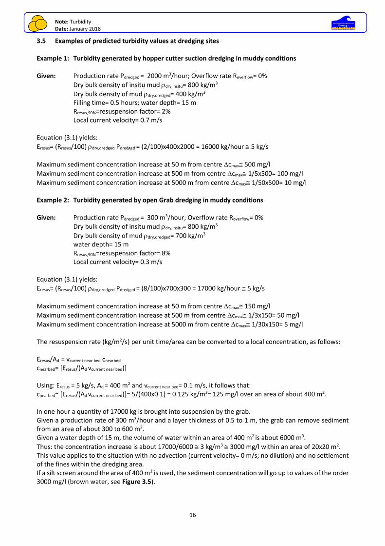
3.5 Examples of predicted turbidity values at dredging sites Example 1: Turbidity generated by hopper cutter suction dredging in muddy conditions Given: Production rate Pdredged = 2000 m3/hour; Overflow rate Roverflow= 0%
Dry bulk density of insitu mud dry,insitu= 800 kg/m3
Dry bulk density of mud dry,dredged= 400 kg/m3 Filling time= 0.5 hours; water depth= 15 m Rresus,90%=resuspension factor= 2% Local current velocity= 0.7 m/s Equation (3.1) yields:
Eresus= (Rresus/100) dry,dredged Pdredged = (2/100)x400x2000 = 16000 kg/hour 5 kg/s
Maximum sediment concentration increase at 50 m from centre cmax 500 mg/l
Maximum sediment concentration increase at 500 m from centre cmax 1/5x500= 100 mg/l
Maximum sediment concentration increase at 5000 m from centre cmax 1/50x500= 10 mg/l Example 2: Turbidity generated by open Grab dredging in muddy conditions Given: Production rate Pdredged = 300 m3/hour; Overflow rate Roverflow= 0%
Dry bulk density of insitu mud dry,insitu= 800 kg/m3
Dry bulk density of mud dry,dredged= 700 kg/m3 water depth= 15 m Rresus,90%=resuspension factor= 8% Local current velocity= 0.3 m/s Equation (3.1) yields:
Eresus= (Rresus/100) dry,dredged Pdredged = (8/100)x700x300 = 17000 kg/hour 5 kg/s
Maximum sediment concentration increase at 50 m from centre cmax 150 mg/l
Maximum sediment concentration increase at 500 m from centre cmax 1/3x150= 50 mg/l
Maximum sediment concentration increase at 5000 m from centre cmax 1/30x150= 5 mg/l The resuspension rate (kg/m2/s) per unit time/area can be converted to a local concentration, as follows: Eresus/Ad = vcurrent near bed cnearbed cnearbed= [Eresus/(Ad vcurrent near bed)] Using: Eresus = 5 kg/s, Ad = 400 m2 and vcurrent near bed= 0.1 m/s, it follows that: cnearbed= [Eresus/(Ad vcurrent near bed)]= 5/(400x0.1) = 0.125 kg/m3= 125 mg/l over an area of about 400 m2. In one hour a quantity of 17000 kg is brought into suspension by the grab. Given a production rate of 300 m3/hour and a layer thickness of 0.5 to 1 m, the grab can remove sediment from an area of about 300 to 600 m2. Given a water depth of 15 m, the volume of water within an area of 400 m2 is about 6000 m3.
Thus: the concentration increase is about 17000/6000 3 kg/m3 3000 mg/l within an area of 20x20 m2. This value applies to the situation with no advection (current velocity= 0 m/s; no dilution) and no settlement of the fines within the dredging area. If a silt screen around the area of 400 m2 is used, the sediment concentration will go up to values of the order 3000 mg/l (brown water, see Figure 3.5).
Note: Turbidity Date: January 2018
17
www.leovanrijn-sediment.com
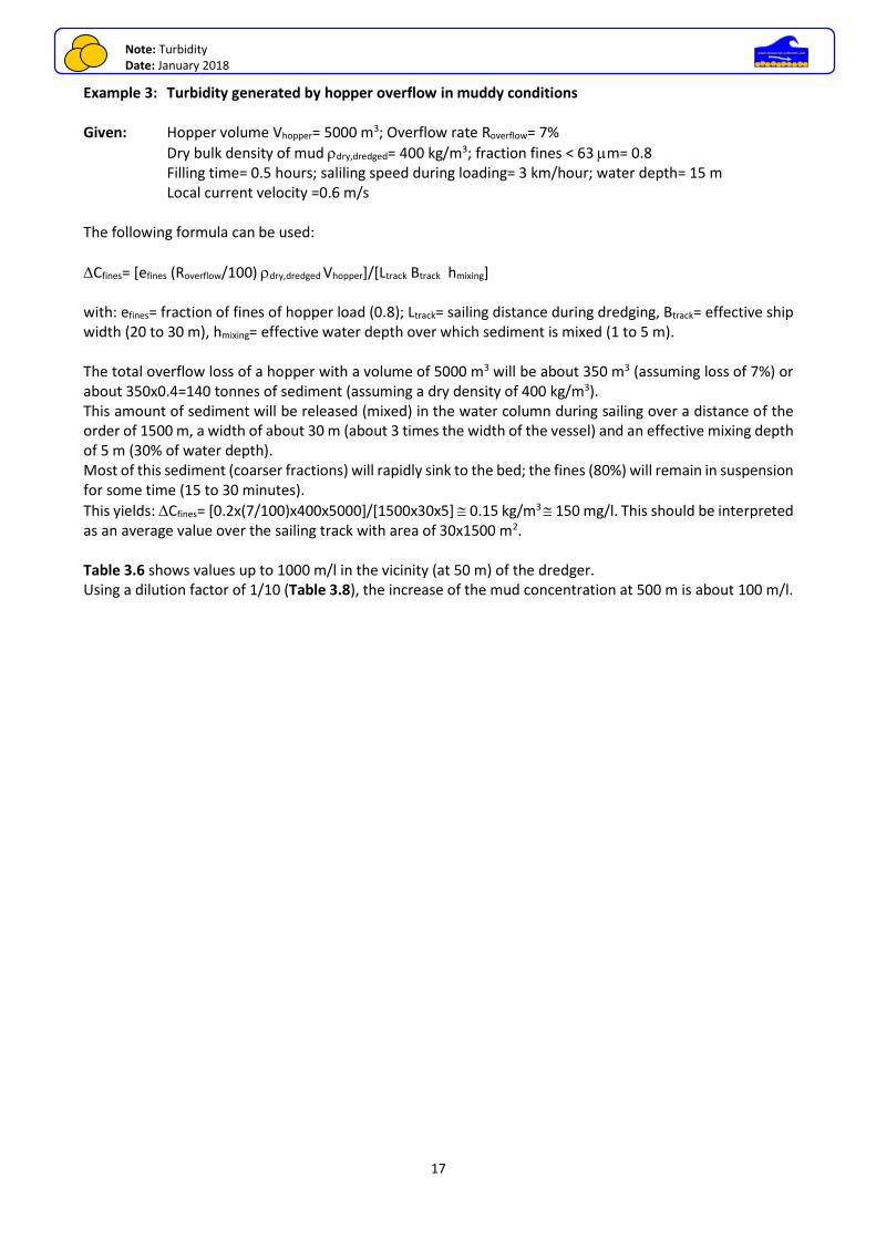
Example 3: Turbidity generated by hopper overflow in muddy conditions Given: Hopper volume Vhopper= 5000 m3; Overflow rate Roverflow= 7%
Dry bulk density of mud dry,dredged= 400 kg/m3; fraction fines < 63 m= 0.8 Filling time= 0.5 hours; saliling speed during loading= 3 km/hour; water depth= 15 m Local current velocity =0.6 m/s The following formula can be used:
Cfines= [efines (Roverflow/100) dry,dredged Vhopper]/[Ltrack Btrack hmixing] with: efines= fraction of fines of hopper load (0.8); Ltrack= sailing distance during dredging, Btrack= effective ship width (20 to 30 m), hmixing= effective water depth over which sediment is mixed (1 to 5 m). The total overflow loss of a hopper with a volume of 5000 m3 will be about 350 m3 (assuming loss of 7%) or about 350x0.4=140 tonnes of sediment (assuming a dry density of 400 kg/m3). This amount of sediment will be released (mixed) in the water column during sailing over a distance of the order of 1500 m, a width of about 30 m (about 3 times the width of the vessel) and an effective mixing depth of 5 m (30% of water depth). Most of this sediment (coarser fractions) will rapidly sink to the bed; the fines (80%) will remain in suspension for some time (15 to 30 minutes).
This yields: Cfines= [0.2x(7/100)x400x5000]/[1500x30x5] 0.15 kg/m3 150 mg/l. This should be interpreted as an average value over the sailing track with area of 30x1500 m2. Table 3.6 shows values up to 1000 m/l in the vicinity (at 50 m) of the dredger. Using a dilution factor of 1/10 (Table 3.8), the increase of the mud concentration at 500 m is about 100 m/l.
Note: Turbidity Date: January 2018
18
www.leovanrijn-sediment.com
4. Turbidity at dumping sites 4.1 Dumping/disposal sites Two options are available for disposal:
• on land (reclamation); - requiring design and construction of dikes; - requiring compaction and drainage of dumped materials;
• open water (river, estuary or coastal sea); - near-field dumping and far-field dumping.
The selection of a dumping site in open water depends on:
• hydrodynamic conditions at the disposal site (wave action and currents should be minimum);
• location of the disposal site with respect to the recirculation of fines to the dredging site (preferably on downdrift side of net current); some recirculation is acceptable as long as the cost of additional dredging is less than disposing it at another site without recirculation; the storage capacity should be sufficient;
Near-field dumping This disposal method is a cheap solution and consists of:
• side-casting at dredging location (channel) resulting in a mound along the channel (relatively high mounds are more easily resuspended); downdrift bypassing (maintenance dredging in a channel through a large shoal can be best dumped at downdrift location so that the sand remains in the system);
• thin-layer disposal over wide area to prevent resuspension and backflow to dredging location (area should be much larger than the dredging area).
Far-field dumping This disposal method is relatively expensive as it is aimed at dumping the sediments as far as possible from the dredging site to prevent sediments from returning to the dredging site. The following methods can be distinguished;
• offshore mounds in deep water; it may be attractive to make an offshore reef protecting the coast landward of the reef (if dredged material is sand);
• nearshore feeder berm; it may be attactive to keep the dredged material (if sandy) in the nearshore system with possible effect of nourishing the beach system.
Unpolluted or lightly polluted dredged material can generally be dumped at a near-field or far-field disposal sites. Very polluted materials should preferably be dumped on land in confined areas. 4.2 Dumping processes in open water The method of dumping strongly depends on the environmental effects (turbidity should be minimum); silts and clays are generally dispersed over relatively large areas in the presence of currents (mud plumes). The resuspension potential at dumping site (stirring up of deposited sediment by local currents and storm waves) should be studied. Most of the disposed materials will sink relatively quickly to the bed as a density current. In shallow water, the deposited sediments can be stirred up easily in relatively shallow water by wind waves. The thickness of the deposits at the dump site should remain relatively small (not more than 10% of local water depth) at the end of the project to minimize resuspension; preferably, the disposal site should be selected at a location where the wave and current-related bed-shear stresses remain relatively small so that the sediments are not dispersed or carried away from the designated limits of the site (Scheffner, 1991).
Note: Turbidity Date: January 2018
19
www.leovanrijn-sediment.com
The available dumping methods are:
• free fall dumping (bulk load) using hopper or barges with bottom doors or split hull hopper/barges;
• continuous jet or plume disposal by pumping of mixture through a floating or submerged pipe (with or without a diffusor) into the water column;
• side casting at dumping site (sediment is pumped from the hopper into the water column at disposal site); submerged or emerged methods can be used;
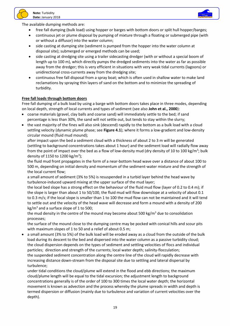
• side casting at dredging site using a trailer sidecasting dredger (with or without a special boom of length up to 100 m), which directly pumps the dredged sediments into the water as far as possible away from the dredger; this is very efficient in situations with very weak tidal currents (lagoons) or unidirectional cross-currents away from the dredging site;
• continuous free fall disposal from a spray boat; which is often used in shallow water to make land reclamations by spraying thin layers of sand on the bottom and to minimize the spreading of turbidity.
Free fall loads through bottom doors Free fall dumping of a bulk load by using a barge with bottom doors takes place in three modes, depending on local depth, strength of local currents and types of sediment (see also John et al., 2000):
• coarse materials (gravel, clay balls and coarse sand) will immediately settle to the bed; if sand percentage is less than 30%, the sand will not settle out, but tends to stay within the slurry;
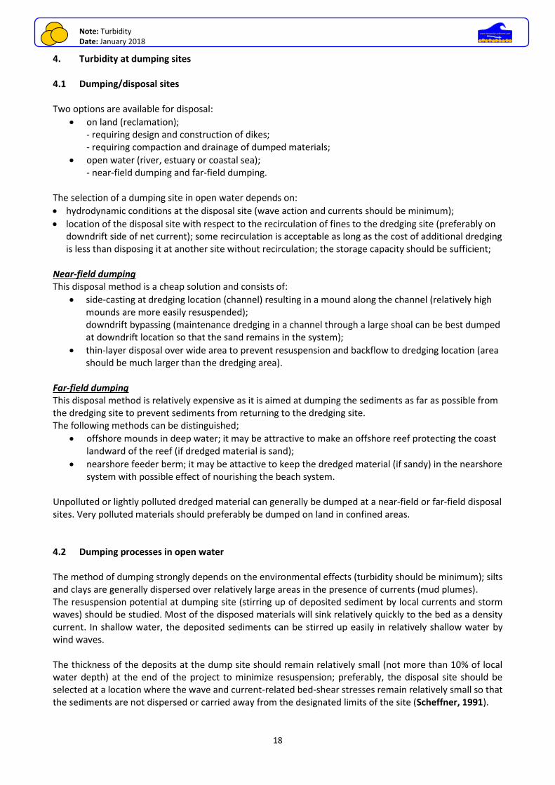
• the vast majority of the fines will also sink (descend) rapidly to the bottom as a bulk load with a cloud settling velocity (dynamic plume phase; see Figure 4.1); where it forms a low-gradient and low-density circular mound (fluid mud mound); after impact upon the bed a sediment cloud with a thickness of about 2 to 3 m will be generated (settling to background concentrations takes about 1 hour) and the sediment load will radially flow away from the point of impact over the bed as a flow of low-density mud (dry density of 10 to 100 kg/m3; bulk density of 1150 to 1200 kg/m3); the fluid mud front propagates in the form of a near-bottom head wave over a distance of about 100 to 500 m, depending on initial density and momentum of the sediment-water mixture and the strength of the local current flow; a small amount of sediment (3% to 5%) is resuspended in a turbid layer behind the head wave by turbulence-induced upward mixing at the upper surface of the mud layer; the local bed slope has a strong effect on the behaviour of the fluid mud flow (layer of 0.2 to 0.4 m); if the slope is larger than about 1 to 50/100, the fluid mud will flow downslope at a velocity of about 0.1 to 0.3 m/s; if the local slope is smaller than 1 to 100 the mud flow can not be maintained and it will tend to settle out and the velocity of the head wave will decrease and form a mound with a density of 200 kg/m3 and a surface slope of 1 to 500; the mud density in the centre of the mound may become about 500 kg/m3 due to consolidation processes; the surface of the mound close to the dumping centre may be pocked with conical hills and scour pits with maximum slopes of 1 to 50 and a relief of about 0.5 m;
• a small amount (3% to 5%) of the bulk load will be eroded away as a cloud from the outside of the bulk load during its descent to the bed and dispersed into the water column as a passive turbidity cloud; the cloud dispersion depends on the types of sediment and settling velocities of flocs and individual particles; direction and strength of the currents; local water depth; salinity-flocculation; the suspended sediment concentration along the centre line of the cloud will rapidly decrease with increasing distance down-stream from the disposal site due to settling and lateral dispersal by turbulence; under tidal conditions the cloud/plume will extend in the flood and ebb directions; the maximum cloud/plume length will be equal to the tidal excursion; the adjustment length to background concentrations generally is of the order of 100 to 300 times the local water depth; the horizontal movement is known as advection and the process whereby the plume spreads in width and depth is termed dispersion or diffusion (mainly due to turbulence and variation of current velocities over the depth).
Note: Turbidity Date: January 2018
20
www.leovanrijn-sediment.com
Jet disposal through submerged pipeline Continuous jet disposal through horizontal or vertical submerged pipelines can take place in two modes (see Figures 4.1, 4.2, 4.3);
• low-concentration mixture pumped into the water column and dispersed over the depth by turbulence and settling due to individual sediments (passive plume moving due to external forces); basic processes are: - segregation of fractions (heterogeneous sediments); larger particles have larger settling velocities; - horizontal advection by wind-driven, tide-driven and wave-driven currents; - lateral diffusion due to turbulent forces generated by currents; modelling techniques are: - random walk models including advection and diffusion; - gaussian diffusion models; - numerical transport models including advection and diffusion;
• high-concentration mixture pumped into the water column behaving as a density jet or as a cloud/plume of particles (cloud settling) descending rapidly to the bed (dynamic plume moving due to internal forces); basic processes are: - initial descent of plume to bottom (cloud or convective settling); - settling from high-concentration near-bottom layers as density current; - horizontal flow of density current along bed; dynamic plume behaviour depends on: - nature of sediment; - density and momentum in descent phase; - degree of aggregation during descent (increased settling velocity).
Figure 4.1 Dynamic and passive plumes at hopper disposal site
Figure 4.2 Side casting of maintenance dredging using a boom dredger in channel
Dynamic plume
(Density current)
Sea bed
Hopper
Passive plume
(Mixing)Sea bed
Hopper
Boom dredger
(up to 100 m)
Side casting
Note: Turbidity Date: January 2018
21
www.leovanrijn-sediment.com
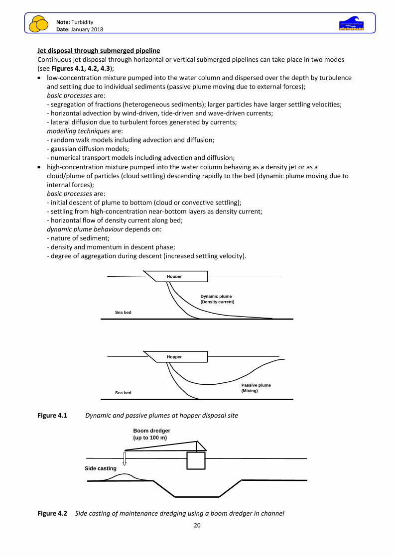
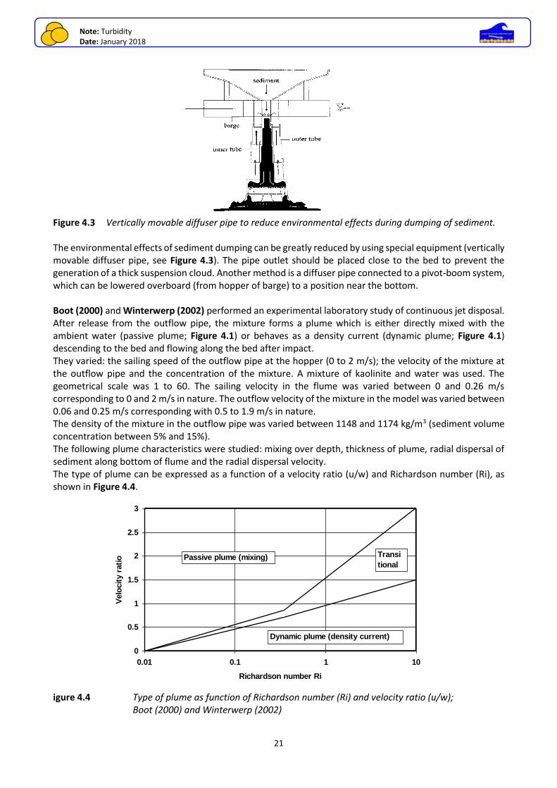
Figure 4.3 Vertically movable diffuser pipe to reduce environmental effects during dumping of sediment. The environmental effects of sediment dumping can be greatly reduced by using special equipment (vertically movable diffuser pipe, see Figure 4.3). The pipe outlet should be placed close to the bed to prevent the generation of a thick suspension cloud. Another method is a diffuser pipe connected to a pivot-boom system, which can be lowered overboard (from hopper of barge) to a position near the bottom. Boot (2000) and Winterwerp (2002) performed an experimental laboratory study of continuous jet disposal. After release from the outflow pipe, the mixture forms a plume which is either directly mixed with the ambient water (passive plume; Figure 4.1) or behaves as a density current (dynamic plume; Figure 4.1) descending to the bed and flowing along the bed after impact. They varied: the sailing speed of the outflow pipe at the hopper (0 to 2 m/s); the velocity of the mixture at the outflow pipe and the concentration of the mixture. A mixture of kaolinite and water was used. The geometrical scale was 1 to 60. The sailing velocity in the flume was varied between 0 and 0.26 m/s corresponding to 0 and 2 m/s in nature. The outflow velocity of the mixture in the model was varied between 0.06 and 0.25 m/s corresponding with 0.5 to 1.9 m/s in nature. The density of the mixture in the outflow pipe was varied between 1148 and 1174 kg/m3 (sediment volume concentration between 5% and 15%). The following plume characteristics were studied: mixing over depth, thickness of plume, radial dispersal of sediment along bottom of flume and the radial dispersal velocity. The type of plume can be expressed as a function of a velocity ratio (u/w) and Richardson number (Ri), as shown in Figure 4.4.
igure 4.4 Type of plume as function of Richardson number (Ri) and velocity ratio (u/w); Boot (2000) and Winterwerp (2002)
0
0.5
1
1.5
2
2.5
3
0.01 0.1 1 10
Richardson number Ri
Velo
cit
y r
ati
o Passive plume (mixing)
Dynamic plume (density current)
Transi
tional

Note: Turbidity Date: January 2018
22
www.leovanrijn-sediment.com
The basic parameters are: u= velocity of ambient water relative to the ship sailing with or against the flow,
w= outflow velocity of mixture (plume) at pipe; Ri= gd/w2 with = (mixture-water)/water , mixture= density of mixture in outflow pipe, g= acceleration of gravity, d= diameter of outflow pipe.
Given the following values as an example calculation: u= 1 m/s, w= 2 m/s, mixture= 1100 kg/m3, water= 1025 kg/m3, d= 1 m; the plume will behave as a density current (Ri= 0.18; u/w= 0.5). Free fall spraying Land reclamations in shallow waters (< 3 m) are often made by using a spraying system connected to a pipeline, see Figures 4.5 and 4.6. The production rate of water + sand is about 0.5 to 1 m3/s for one pipeline. The pipeline concentration of sand is of the order of 200 to 300 kg/m3. The spraying system continuously moves forward along the land reclamation area. Thin layers of sand are produced until the top level of the new sand area is close to the waterline. After that, the spraying boat is removed and the pipeline exit is placed directly on the sediment bottom. Small dikes are made by bulldozers and excavators to prevent the lateral spreading of the sediment mixture. The spraying method is prefered in conditions with relatively soft subsoils so that the consolidation process of the subsoil can proceed gradually. The vertical spraying system is most suitable for small-scale land reclamations (in lakes) and produces less turbidity in the surroundings. The horizontal spraying system is most suitable for marine conditions (nearshore mounds; nearshore bars; under water nourishments).
Figure 4.5 Vertical spraying system
Figure 4.6 Horizontal spraying system
sand supply by pipeline spray system
spray mixture under water
sediment bottom
clouds of fine sediment generated in suspension
5 m
sand supply by pipeline
mixture dilution under water
sediment bottom
clouds of fine sediment generated in suspension
10-15 m
Note: Turbidity Date: January 2018
23
www.leovanrijn-sediment.com
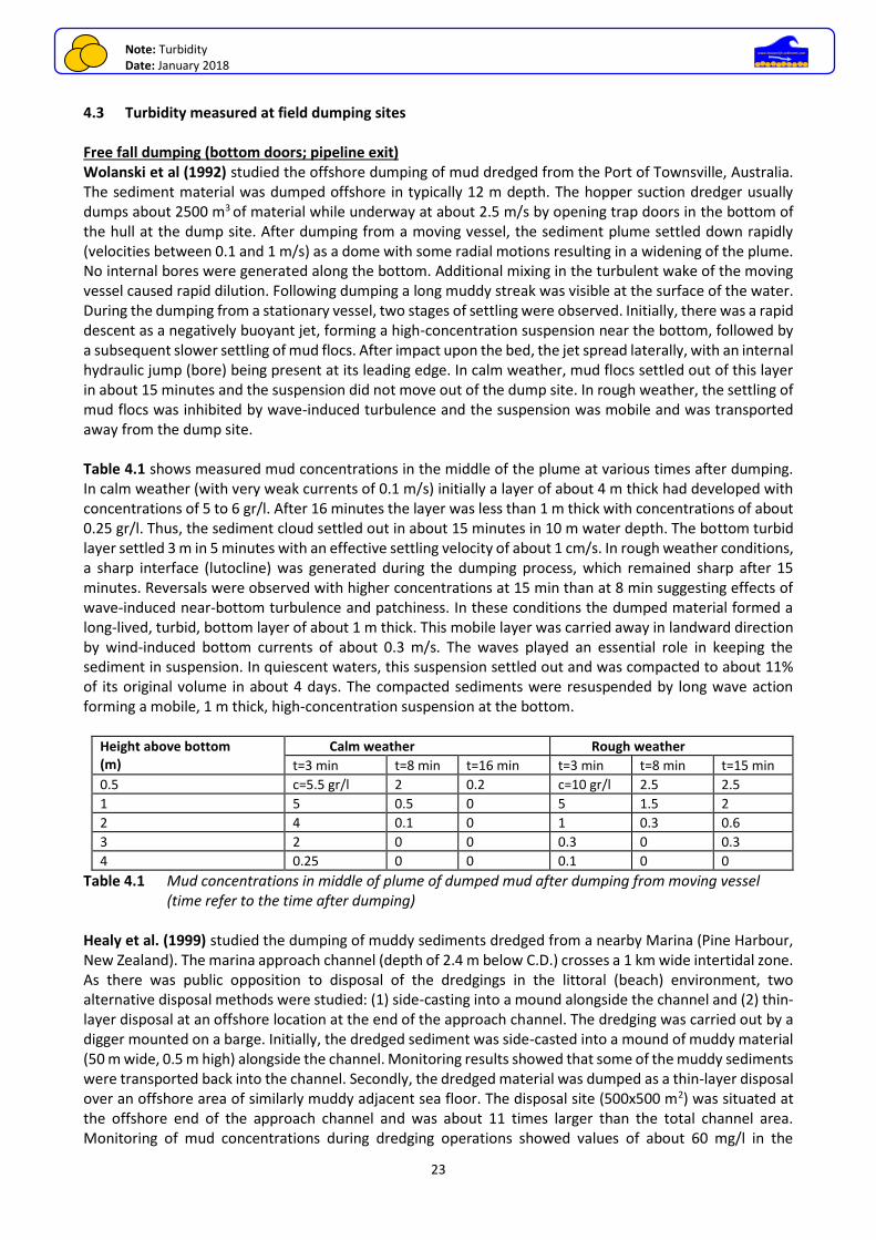
4.3 Turbidity measured at field dumping sites Free fall dumping (bottom doors; pipeline exit) Wolanski et al (1992) studied the offshore dumping of mud dredged from the Port of Townsville, Australia. The sediment material was dumped offshore in typically 12 m depth. The hopper suction dredger usually dumps about 2500 m3 of material while underway at about 2.5 m/s by opening trap doors in the bottom of the hull at the dump site. After dumping from a moving vessel, the sediment plume settled down rapidly (velocities between 0.1 and 1 m/s) as a dome with some radial motions resulting in a widening of the plume. No internal bores were generated along the bottom. Additional mixing in the turbulent wake of the moving vessel caused rapid dilution. Following dumping a long muddy streak was visible at the surface of the water. During the dumping from a stationary vessel, two stages of settling were observed. Initially, there was a rapid descent as a negatively buoyant jet, forming a high-concentration suspension near the bottom, followed by a subsequent slower settling of mud flocs. After impact upon the bed, the jet spread laterally, with an internal hydraulic jump (bore) being present at its leading edge. In calm weather, mud flocs settled out of this layer in about 15 minutes and the suspension did not move out of the dump site. In rough weather, the settling of mud flocs was inhibited by wave-induced turbulence and the suspension was mobile and was transported away from the dump site. Table 4.1 shows measured mud concentrations in the middle of the plume at various times after dumping. In calm weather (with very weak currents of 0.1 m/s) initially a layer of about 4 m thick had developed with concentrations of 5 to 6 gr/l. After 16 minutes the layer was less than 1 m thick with concentrations of about 0.25 gr/l. Thus, the sediment cloud settled out in about 15 minutes in 10 m water depth. The bottom turbid layer settled 3 m in 5 minutes with an effective settling velocity of about 1 cm/s. In rough weather conditions, a sharp interface (lutocline) was generated during the dumping process, which remained sharp after 15 minutes. Reversals were observed with higher concentrations at 15 min than at 8 min suggesting effects of wave-induced near-bottom turbulence and patchiness. In these conditions the dumped material formed a long-lived, turbid, bottom layer of about 1 m thick. This mobile layer was carried away in landward direction by wind-induced bottom currents of about 0.3 m/s. The waves played an essential role in keeping the sediment in suspension. In quiescent waters, this suspension settled out and was compacted to about 11% of its original volume in about 4 days. The compacted sediments were resuspended by long wave action forming a mobile, 1 m thick, high-concentration suspension at the bottom.
Height above bottom (m)
Calm weather Rough weather
t=3 min t=8 min t=16 min t=3 min t=8 min t=15 min
0.5 c=5.5 gr/l 2 0.2 c=10 gr/l 2.5 2.5
1 5 0.5 0 5 1.5 2
2 4 0.1 0 1 0.3 0.6
3 2 0 0 0.3 0 0.3
4 0.25 0 0 0.1 0 0
Table 4.1 Mud concentrations in middle of plume of dumped mud after dumping from moving vessel (time refer to the time after dumping)
Healy et al. (1999) studied the dumping of muddy sediments dredged from a nearby Marina (Pine Harbour, New Zealand). The marina approach channel (depth of 2.4 m below C.D.) crosses a 1 km wide intertidal zone. As there was public opposition to disposal of the dredgings in the littoral (beach) environment, two alternative disposal methods were studied: (1) side-casting into a mound alongside the channel and (2) thin- layer disposal at an offshore location at the end of the approach channel. The dredging was carried out by a digger mounted on a barge. Initially, the dredged sediment was side-casted into a mound of muddy material (50 m wide, 0.5 m high) alongside the channel. Monitoring results showed that some of the muddy sediments were transported back into the channel. Secondly, the dredged material was dumped as a thin-layer disposal over an offshore area of similarly muddy adjacent sea floor. The disposal site (500x500 m2) was situated at the offshore end of the approach channel and was about 11 times larger than the total channel area. Monitoring of mud concentrations during dredging operations showed values of about 60 mg/l in the
Note: Turbidity Date: January 2018
24
www.leovanrijn-sediment.com
dredging plume just north of the channel, while background values were of the order of 30 mg/l. Monitoring of mud concentrations during dumping of sediments (from a barge) at the disposal site showed values of 50 to 70 mg/l in the trailing plume from the barge. At distances greater than 250 m from the barge the mud concentrations were close to background values (about 20 mg/l). The turbid plume was observed to be a transient feature which typically lasted 5 to 15 minutes. The maximum thickness of the mud layer on the sea floor was about 0.3 m per year in the central disposal area and no mounds of muddy deposits accumulated. Spanhoff et al., 1990 studied the recirculation of fine sediments dumped at an offshore mud disposal site ‘Loswal Noord’ near the entrance (at about 11 km) to the Port of Rotterdam, The Netherlands. Large quantities (15 to 20 million m3 per year) of sediment (mud and fine sand) dredged from the harbour basins are dumped at this site. The sea bottom at the site is relatively flat outside the dump area. The water depths vary in the range of 15 to 20 m below mean sea level. The tidal range is about 2 m; the peak tidal flood currents to the north are about 0.7 m/s and the peak tidal ebb currents to the south are about 0.6 m/s. The fresh-water river outflow from the Rhine is about 1500 m3/s generating a stratified flow system over an offshore distance of about 11 km from the entrance. Residual currents (order of 0.05 m/s) near the bottom at the dump site are found to be directed landward to the river outlet. As the sediments at the dump sites are confined to the lower layers, there is a potential for recirculation of sediment back to the dredging sites (harbour basins). Results from mass balance studies (comparison of total dumped volume and sedimentation volume of the in-situ mound at seabottom) over about 20 years show that about 50% to 80% of the dumped mud and about 30% of the fine sand has been carried away from the dump site in alongshore directions. Mathematical model studies (3D) suggest the presence of a relatively strong return flow of mud from the dump site towards the harbour entrance largely due to the generation of a large-scale horizontal gyre and the presence of vertical circulation due to salinity-induced density gradients. Free fall spraying
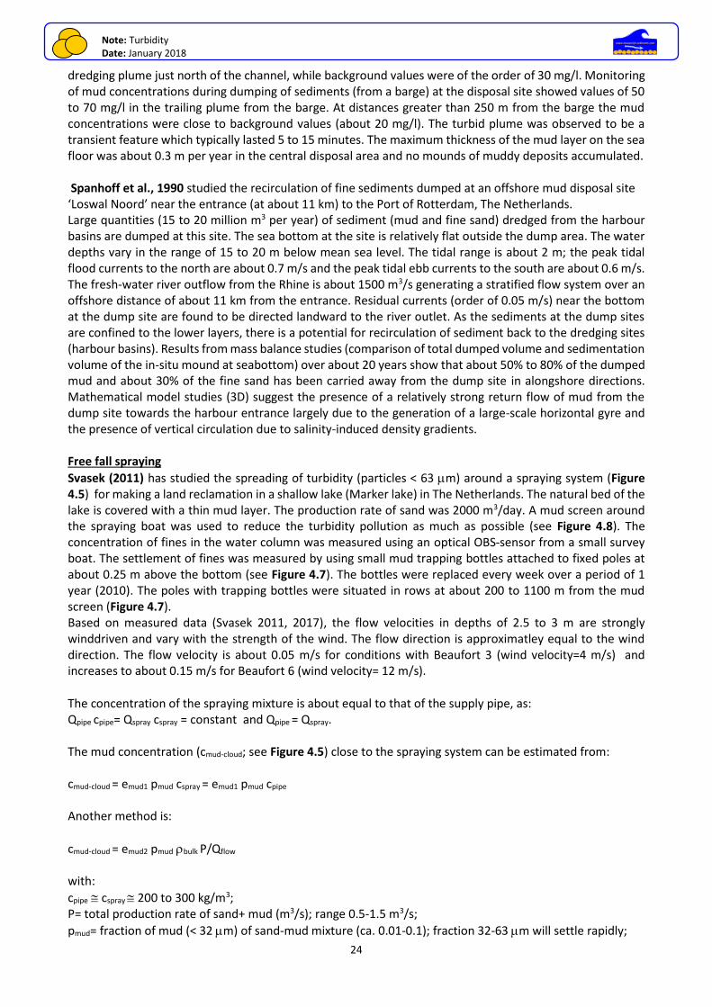
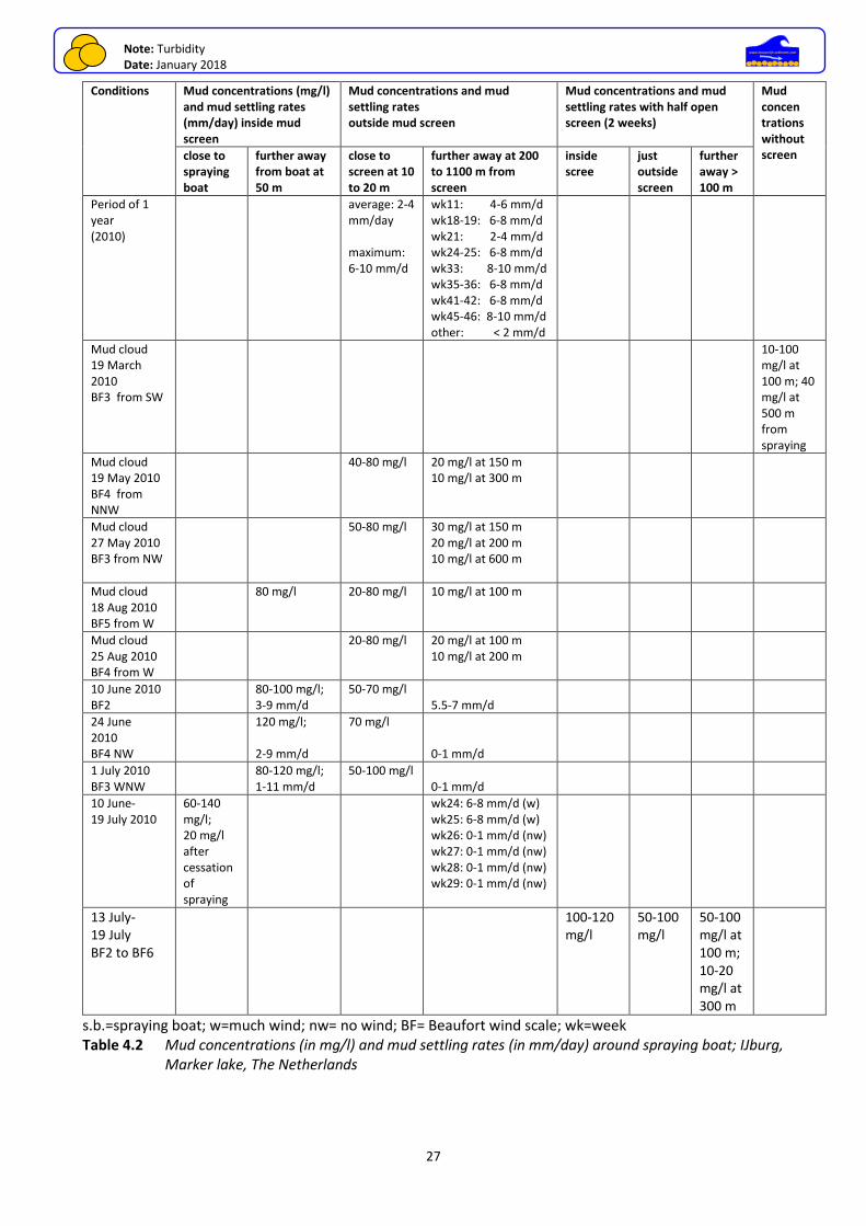
Svasek (2011) has studied the spreading of turbidity (particles < 63 m) around a spraying system (Figure 4.5) for making a land reclamation in a shallow lake (Marker lake) in The Netherlands. The natural bed of the lake is covered with a thin mud layer. The production rate of sand was 2000 m3/day. A mud screen around the spraying boat was used to reduce the turbidity pollution as much as possible (see Figure 4.8). The concentration of fines in the water column was measured using an optical OBS-sensor from a small survey boat. The settlement of fines was measured by using small mud trapping bottles attached to fixed poles at about 0.25 m above the bottom (see Figure 4.7). The bottles were replaced every week over a period of 1 year (2010). The poles with trapping bottles were situated in rows at about 200 to 1100 m from the mud screen (Figure 4.7). Based on measured data (Svasek 2011, 2017), the flow velocities in depths of 2.5 to 3 m are strongly winddriven and vary with the strength of the wind. The flow direction is approximatley equal to the wind direction. The flow velocity is about 0.05 m/s for conditions with Beaufort 3 (wind velocity=4 m/s) and increases to about 0.15 m/s for Beaufort 6 (wind velocity= 12 m/s).
The concentration of the spraying mixture is about equal to that of the supply pipe, as: Qpipe cpipe= Qspray cspray = constant and Qpipe = Qspray. The mud concentration (cmud-cloud; see Figure 4.5) close to the spraying system can be estimated from: cmud-cloud = emud1 pmud cspray = emud1 pmud cpipe Another method is:
cmud-cloud = emud2 pmud bulk P/Qflow with:
cpipe cspray 200 to 300 kg/m3; P= total production rate of sand+ mud (m3/s); range 0.5-1.5 m3/s;
pmud= fraction of mud (< 32 m) of sand-mud mixture (ca. 0.01-0.1); fraction 32-63 m will settle rapidly;
Note: Turbidity Date: January 2018
25
www.leovanrijn-sediment.com
cpipe = mud concentration in supply pipeline (200 to 300 kg/m3);
bulk= bulk density of sand-mud mixture ( 1600 kg/m3); Qflow= b h u= flow discharge passing the spraying boat;
b= size of spraying boat ( 10 m); h= local water depth; u= local flow velocity; emud1= mud loss factor (0.01-0.05); mud loss from outer spray layer under water (about 10%); outer layer is about 20% of total spray layer; emud2= mud loss factor (0.01-0.05). Measured data of Savsek (2011):
cmud-cloud 150 mg/l 0.15 kg/m3; pmud 0.05, P= 0.11 m3/s (16000 m3/week; 40 hours);
Qflow=bhu=10x3x0.1 = 3 m3/s; cpipe 250 kg/m3 yielding: emud1 0.15/(0.05x250) 0.01;
emud2 0.15x3/(0.05x1600x0.11)= 0.05
Figure 4.7 Location of measuring poles (black dots) with mud trapping bottles (right) and mud screen
(yellow); A, B, C and D are fixed poles within the screen area (Svasek 2011)
Based on the analysis of measured mud concentrations (in mg/liter) and mud settlling rates (in mm/day), the following conclusions are given (see also Table 4.2):
• mud concentrations are approximately uniform over the water depth (2.5 to 3 m); the natural mud concentrations in conditions without spraying of sand are about 10 mg/l in conditions with almost no wind (BF <3) and about 40 mg/l with much wind (BF 6);
• mud settllement in conditions without spraying of sand is about 0 to 4 mm/day with little wind and 8-14 mm/day with much wind;
• mud settlement values at a distance of 200 to 1100 m from the mud screen are: - average settlement over a year of about 3 mm/day; variation of 0 mm/days in periods with no wind to 14 mm/day in periods with much wind; - variation of settlement is relatively large due to influence of waves stirring mud from the bottom at windy days; - influence of spraying system on the turbidity levels outside the screen is limited to a circle of about 200 m around the screen, where increased mud settling rates and concentrations do occur;
• maximum mud concentrations inside the screen area are 60 to 120 mg/l at distance of 25 to 50 m from the spraying boat; mud settling close to spraying boat is 9-11 mm/day and 1-3 mm/day at distance of 25 to 50 m from spraying boat;
Note: Turbidity Date: January 2018
26
www.leovanrijn-sediment.com
• maximum mud concentrations just outside mud screen are 30 tot 60 mg/l during conditions with no wind (BF < 3) and 100 mg/l with much wind (BF 5-6); mud settlement just outside screen is 2 mm/day with no wind and 8 mm/day with much wind;
• mud screen yields maximum concentration reduction of 50% in conditions with no wind and 25% reduction in conditions with much wind; relatively much turbidity passes the sreen on windy days;
• mud clouds with initial concentration of about 100 mg/l inside the mud screen reduce to about 10 mg/l (natural background concentration) over distance of about 200 m (dilution factor 1/10); natural concentrations are present at distances > 200 m from the screen;
• mud clouds with initial concentration of about 100 mg/l near the spraying boat (without mud screen) reduce to about 10 mg/l (natural background concentration) over distance of about 400 m (dilution factor 1/10);
• mud clouds are local and temporary phenomena; areas with relatively clear water (concentrations < 10 mg/l) are present inside and outside the sreen at arbitrary locations and times.
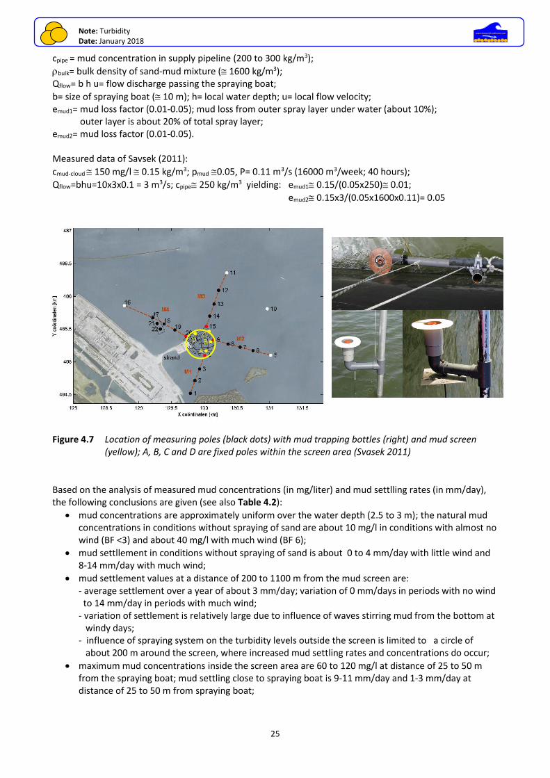
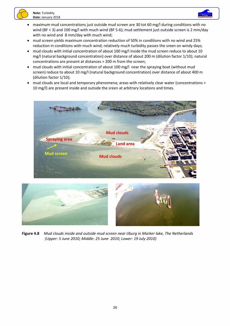
Figure 4.8 Mud clouds inside and outside mud screen near IJburg in Marker lake, The Netherlands
(Upper: 5 June 2010; Middle: 25 June 2010; Lower: 19 July 2010)
Mud screen Mud clouds
Mud clouds
Land area Spraying area
Note: Turbidity Date: January 2018
27
www.leovanrijn-sediment.com
Conditions Mud concentrations (mg/l) and mud settling rates (mm/day) inside mud screen
Mud concentrations and mud settling rates outside mud screen
Mud concentrations and mud settling rates with half open screen (2 weeks)
Mud concen trations without screen close to
spraying boat
further away from boat at 50 m
close to screen at 10 to 20 m
further away at 200 to 1100 m from screen
inside scree
just outside screen
further away > 100 m
Period of 1 year (2010)
average: 2-4 mm/day maximum: 6-10 mm/d
wk11: 4-6 mm/d wk18-19: 6-8 mm/d wk21: 2-4 mm/d wk24-25: 6-8 mm/d wk33: 8-10 mm/d wk35-36: 6-8 mm/d wk41-42: 6-8 mm/d wk45-46: 8-10 mm/d other: < 2 mm/d
Mud cloud 19 March 2010 BF3 from SW
10-100 mg/l at 100 m; 40 mg/l at 500 m from spraying
Mud cloud 19 May 2010 BF4 from NNW
40-80 mg/l 20 mg/l at 150 m 10 mg/l at 300 m
Mud cloud 27 May 2010 BF3 from NW
50-80 mg/l 30 mg/l at 150 m 20 mg/l at 200 m 10 mg/l at 600 m
Mud cloud 18 Aug 2010 BF5 from W
80 mg/l 20-80 mg/l 10 mg/l at 100 m
Mud cloud 25 Aug 2010 BF4 from W
20-80 mg/l 20 mg/l at 100 m 10 mg/l at 200 m
10 June 2010 BF2
80-100 mg/l; 3-9 mm/d
50-70 mg/l 5.5-7 mm/d
24 June 2010 BF4 NW
120 mg/l; 2-9 mm/d
70 mg/l 0-1 mm/d
1 July 2010 BF3 WNW
80-120 mg/l; 1-11 mm/d
50-100 mg/l 0-1 mm/d
10 June- 19 July 2010
60-140 mg/l; 20 mg/l after cessation of spraying
wk24: 6-8 mm/d (w) wk25: 6-8 mm/d (w) wk26: 0-1 mm/d (nw) wk27: 0-1 mm/d (nw) wk28: 0-1 mm/d (nw) wk29: 0-1 mm/d (nw)
13 July- 19 July BF2 to BF6
100-120 mg/l
50-100 mg/l
50-100 mg/l at 100 m; 10-20 mg/l at 300 m
s.b.=spraying boat; w=much wind; nw= no wind; BF= Beaufort wind scale; wk=week Table 4.2 Mud concentrations (in mg/l) and mud settling rates (in mm/day) around spraying boat; IJburg,
Marker lake, The Netherlands
Note: Turbidity Date: January 2018
28
www.leovanrijn-sediment.com
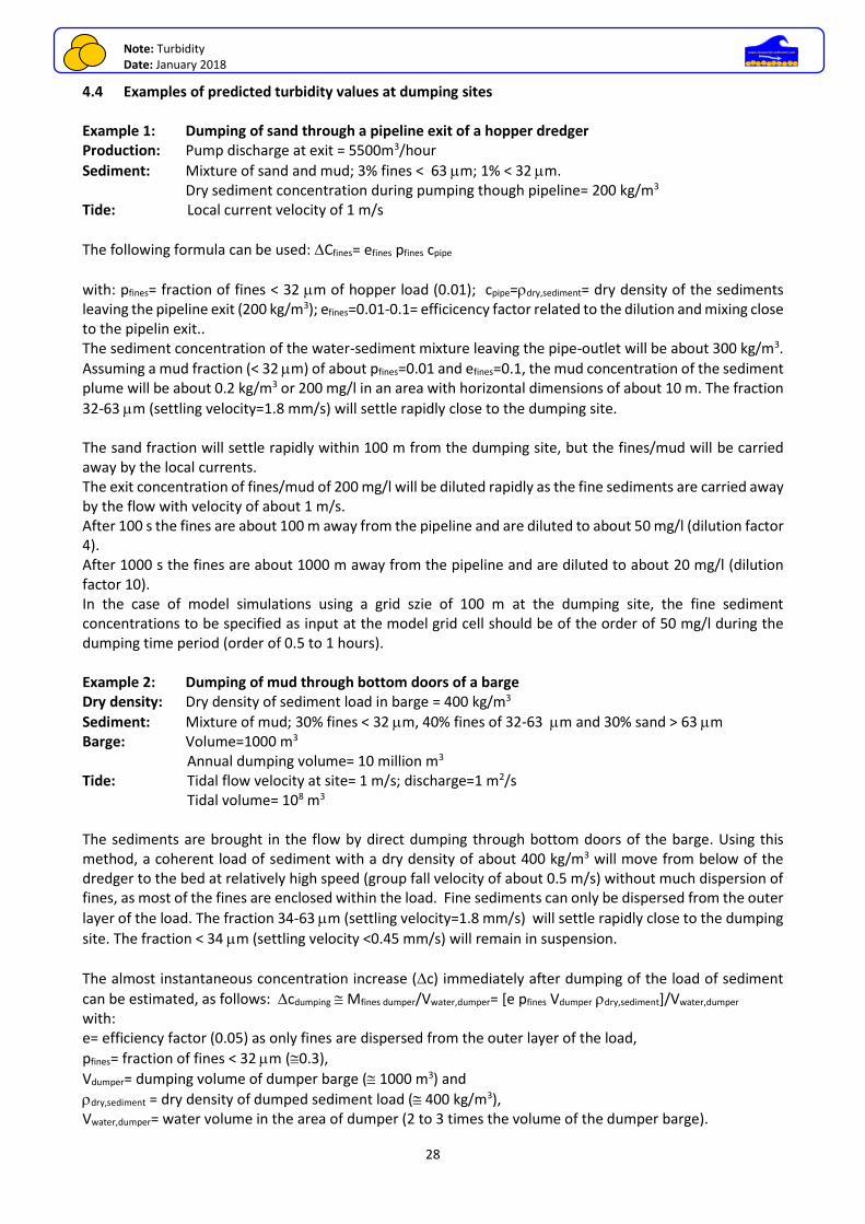
4.4 Examples of predicted turbidity values at dumping sites Example 1: Dumping of sand through a pipeline exit of a hopper dredger Production: Pump discharge at exit = 5500m3/hour
Sediment: Mixture of sand and mud; 3% fines < 63 m; 1% < 32 m. Dry sediment concentration during pumping though pipeline= 200 kg/m3
Tide: Local current velocity of 1 m/s
The following formula can be used: Cfines= efines pfines cpipe
with: pfines= fraction of fines < 32 m of hopper load (0.01); cpipe=dry,sediment= dry density of the sediments leaving the pipeline exit (200 kg/m3); efines=0.01-0.1= efficicency factor related to the dilution and mixing close to the pipelin exit.. The sediment concentration of the water-sediment mixture leaving the pipe-outlet will be about 300 kg/m3.
Assuming a mud fraction (< 32 m) of about pfines=0.01 and efines=0.1, the mud concentration of the sediment plume will be about 0.2 kg/m3 or 200 mg/l in an area with horizontal dimensions of about 10 m. The fraction
32-63 m (settling velocity=1.8 mm/s) will settle rapidly close to the dumping site. The sand fraction will settle rapidly within 100 m from the dumping site, but the fines/mud will be carried away by the local currents. The exit concentration of fines/mud of 200 mg/l will be diluted rapidly as the fine sediments are carried away by the flow with velocity of about 1 m/s. After 100 s the fines are about 100 m away from the pipeline and are diluted to about 50 mg/l (dilution factor 4). After 1000 s the fines are about 1000 m away from the pipeline and are diluted to about 20 mg/l (dilution factor 10). In the case of model simulations using a grid szie of 100 m at the dumping site, the fine sediment concentrations to be specified as input at the model grid cell should be of the order of 50 mg/l during the dumping time period (order of 0.5 to 1 hours). Example 2: Dumping of mud through bottom doors of a barge Dry density: Dry density of sediment load in barge = 400 kg/m3
Sediment: Mixture of mud; 30% fines < 32 m, 40% fines of 32-63 m and 30% sand > 63 m Barge: Volume=1000 m3
Annual dumping volume= 10 million m3 Tide: Tidal flow velocity at site= 1 m/s; discharge=1 m2/s Tidal volume= 108 m3 The sediments are brought in the flow by direct dumping through bottom doors of the barge. Using this method, a coherent load of sediment with a dry density of about 400 kg/m3 will move from below of the dredger to the bed at relatively high speed (group fall velocity of about 0.5 m/s) without much dispersion of fines, as most of the fines are enclosed within the load. Fine sediments can only be dispersed from the outer
layer of the load. The fraction 34-63 m (settling velocity=1.8 mm/s) will settle rapidly close to the dumping
site. The fraction < 34 m (settling velocity <0.45 mm/s) will remain in suspension.
The almost instantaneous concentration increase (c) immediately after dumping of the load of sediment
can be estimated, as follows: cdumping Mfines dumper/Vwater,dumper= [e pfines Vdumper dry,sediment]/Vwater,dumper with: e= efficiency factor (0.05) as only fines are dispersed from the outer layer of the load,
pfines= fraction of fines < 32 m (0.3),
Vdumper= dumping volume of dumper barge ( 1000 m3) and
dry,sediment = dry density of dumped sediment load ( 400 kg/m3), Vwater,dumper= water volume in the area of dumper (2 to 3 times the volume of the dumper barge).
Note: Turbidity Date: January 2018
29
www.leovanrijn-sediment.com
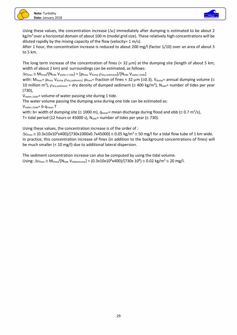
Using these values, the concentration increase (c) immediately after dumping is estimated to be about 2 kg/m3 over a horizontal domain of about 100 m (model grid size). These relatively high concentrations will be diluted rapidly by the mixing capacity of the flow (velocity= 1 m/s). After 1 hour, the concentration increase is reduced to about 200 mg/l (factor 1/10) over an area of about 3 to 5 km.
The long term increase of the concentration of fines (< 32 m) at the dumping site (length of about 5 km; width of about 2 km) and surroundings can be estimated, as follows:
cfines Mfines/(Ntide Vwater,1 tide) = [pfines Vdump dry,sediment]/[Ntide Vwater,1tide]
with: Mfines= pfines Vdump dry,sediment; pfines= fraction of fines < 32 m (0.3), Vdump= annual dumping volume (
10 million m3), dry,sediment = dry density of dumped sediment ( 400 kg/m3), Ntide= number of tides per year (730), Vwater,1tide= volume of water passing site during 1 tide. The water volume passing the dumping area during one tide can be estimated as: Vwater,1tide= b qmean T
with: b= width of dumping site ( 1000 m), qmean= mean discharge during flood and ebb ( 0.7 m2/s),
T= tidal period (12 hours or 45000 s), Ntide= number of tides per year ( 730). Using these values, the concentration increase is of the order of :
cfines (0.3x10x106x400)/(730x1000x0.7x45000) 0.05 kg/m3 50 mg/l for a tidal flow tube of 1 km wide. In practice, this concentration increase of fines (in addition to the background concentrations of fines) will be much smaller (< 10 mg/l) due to additional lateral dispersion. The sediment concentration increase can also be computed by using the tidal volume.
Using: cfines Mfines/[Ntide Vtidalvolume] = (0.3x10x106x400)/(730x 108) 0.02 kg/m3 20 mg/l.
Note: Turbidity Date: January 2018
30
www.leovanrijn-sediment.com
5. Numerical simulation of dispersion and settling processes 5.1 Theory of diffusion/dispersion/dilution processes Dispersion refers to the spreading of very fine sediment mass with a very small settling velocity (almost zero) as a bulk property (averaged concentrations) integrating all spreading/dispersion processes. Generally, the dispersion coefficient including all effects is larger than the turbulent mixing coefficient. Diffusive type of
transport (i c/xi) is also known as Fickian transport.
The 2DV-dimensional advection-dispersion process of fine sediments < 63 m in a horizontally uniform flow (dh/dx=0, du/dx=0) can be described by:
c/t + u c/x – ws c/z – z 2c/z2– x 2c/x2 = 0 (5.1) with: c= sediment concentration, u= flow velocity (constant in space and time), ws= settling velocity of
sediment, = effective diffusion/mixing coefficient (assumed to be constant in space and time; about 0.1 to 10 m2/s; K= dispersion coefficient including other effects), x=longitudinal coordinate, z=vertical coordinate. Equation (5.1) can only be solved numerically.
The concentration of very fine mud (< 8 m) with almost zero settling velocity (< 0.1 m/s) is uniform over the depth. Neglecting the settling velocity and vertical diffusive transport, Equation (5.1) can be expressed as:
c/t + u c/x – x 2c/x2 = 0 (5.2) Assuming a fluid at rest (u= 0), the expression becomes:
c/t - 2c/x2 = 0 (5.3) When a mass M (in kg/m2) is released at x= 0 at time t= 0 as a line source (per unit width) in a channel with constant depth h (channel width=1 m), the solution of the 1-dimensional diffusion equation is:
c= M/(4 t)0.5 exp[–{x/(4 t)0.5}2] (5.4)
with: c= depth-mean concentration (kg/m3), t= time, = constant diffusion/mixing coefficient (m2/s).
Continuity requires that: M = h – c dx (in kg/m2).
Using: x=ut, it follows that: M = h t1t2 uc dt = uh t1t2 c dt = q t1t2 c dt, with t1 and t2 being the leading and trailing edges of the cloud. If the coordinate system is moving with the mean velocity u, then the solution of Equation (5.4) representing a symmetrical solution is also valid with respect to the moving coordinate system. The solution reads:
c= M/(4 t)0.5 exp[–{x’/(4 t)0.5}2] (5.5)
Defining x = ut +x’ (see Figure 5.1) and thus x’= x-ut, it follows that:
c= M/(4 t)0.5 exp[–{(x-ut)/(4 t)0.5}2] =cmax exp[–{(x-ut)/(4 t)0.5}2] (5.6)
with: cmax = M/(4 t)0.5= peak value of the concentration at x=ut.
Thus: cmax = at t= 0 and cmax decreases with 1/( t)0.5; see Table 5.1. Using x=ut: cmax decreases with 1/x0.5.
The solution represents a Gaussian distribution, which reads as: y=[22]-0.5 exp{-(x-)2/(22}.
This yields: 22 = 4 t or = 2/(2t)
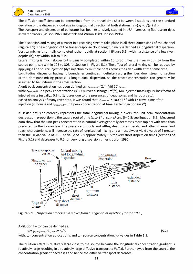
Note: Turbidity Date: January 2018
31
www.leovanrijn-sediment.com
The diffusion coefficient can be determined from the travel time (t) between 2 stations and the standard
deviation of the dispersed cloud size in longitudinal direction at both stations: =(22-1
2)/(2 t). The transport and dispersion of pollutants has been extensively studied in USA-rivers using fluorescent dyes as water tracers (Wilson 1968, Kilpatrick and Wilson 1989, Jobson 1996). The dispersion and mixing of a tracer in a receiving stream take place in all three dimensions of the channel (Figure 5.1). The elongation of the tracer-response cloud longitudinally is defined as longitudinal dispersion. Vertical mixing is normally completed rather rapidly at section I (Figure 5.1), within a distance of a few river depths (h); say within 10h to 30h. Lateral mixing is much slower but is usually completed within 10 to 30 times the river width (B) from the source point; say within 10B to 30B (at Section III, Figure 5.1). The effect of lateral mixing can be reduced by applying a line source injection (dye injection by multiple boats across the river width at the same time). Longitudinal dispersion having no boundaries continues indefinitely along the river; downstream of section III the dominant mixing process is longitudinal dispersion, so the tracer concentration can generally be assumed to be uniform in the cross section. A unit peak concentration has been defined as: cmax,unit=[Q/(r M)] 106 cmax, with: cmax,unit= unit peak concentration (s-1), Q= river discharge (m3/s), M= injected mass (kg), r= loss factor of
injected mass (usually 0.9 to 1; losses due to the presences of dead zones and harbours etc). Based on analysis of many river data, it was found that: cmax,unit,T= 1000 T-0.9 with T= travel time after injection (in hours) and cmax,unit,T= unit peak concentration at time T after injection (in s-1). If Fickian diffusion correctly represents the total longitudinal mixing in rivers, the unit-peak concentration
decreases in proportion to the square root of time (cunitt- or cunitx- and = 0.5; see Equation 5.6). Measured data show that the unit-peak concentration in natural rivers generally decreases more rapidly with time than predicted by the Fickian law. The presence of pools and riffles, dead zones, bends, and other channel and reach characteristics will increase the rate of longitudinal mixing and almost always yield a value of β greater than the Fickian value of 0.5. The value of β is approximately 1.5 for very short dispersion times (section I of Figure 5.1) and decreases to 0.5 for very long dispersion times (Jobson 1996).
Figure 5.1 Dispersion processes in a river from a single-point injection (Jobson 1996) A dilution factor can be defined as:
d= d,longitudinal d,lateral = cx/co (5.7)
with: cx= concentration at location x and co= source concentration; d- values in Table 5.1. The dilution effect is relatively large close to the source because the longitudinal concentration gradient is
relatively large resulting in a relatively large diffusive transport ( c/x). Further away from the source, the concentration gradient decreases and hence the diffusive transport decreases.
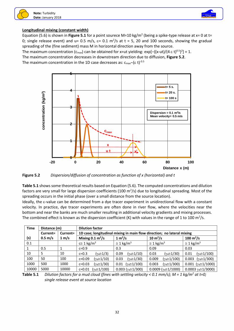
Note: Turbidity Date: January 2018
32
www.leovanrijn-sediment.com
Longitudinal mixing (constant width) Equation (5.6) is shown in Figure 5.1 for a point sourece M=10 kg/m2 (being a spike-type release at x= 0 at t=
0; single release event) and u= 0.5 m/s, = 0.1 m2/s at t = 5, 20 and 100 seconds, showing the gradual spreading of the (fine sediment) mass M in horizontal direction away from the source.
The maximum concentration (cmax) can be obtained for x=ut yielding: exp[–{(x-ut)/(4 t)0.5}2] = 1. The maximum concentration decreases in downstream direction due to diffusion, Figure 5.2.
The maximum concentration in the 1D case decreases as: cmax( t)-0.5
Figure 5.2 Dispersion/diffusion of concentration as function of x (horizontal) and t Table 5.1 shows some theoretical results based on Equation (5.6). The computed concentrations and dilution factors are very small for large dispersion coefficients (100 m2/s) due to longitudinal spreading. Most of the spreading occurs in the initial phase (over a small distance from the source location).
Ideally, the -value can be determined from a dye tracer experiment in unidirectional flow with a constant velocity. In practice, dye tracer experiments are often done in river flow, where the velocities near the bottom and near the banks are much smaller resulting in additional velocity gradients and mixing processes. The combined effect is known as the dispersion coefficient (K) with values in the range of 1 to 100 m2/s.
Time (s)
Distance (m) Dilution factor
Current= 0.5 m/s
Current= 1 m/s
1D case; longitudinal mixing in main flow direction; no lateral mixing
Mixing 0.1 m2/s 1 m2/s 10 m2/s 100 m2/s
0.1 c 1 kg/m3 1 kg/m3 1 kg/m3 1 kg/m3
1 0.5 1 c=0.9 0.3 0.09 0.03
10 5 10 c=0.3 (d1/3) 0.09 (d1/10) 0.03 (d1/30) 0.01 (d1/100)
100 50 100 c=0.09 (d1/10) 0.03 (d1/30) 0.009 (d1/100) 0.003 (d1/300)
1000 500 1000 c=0.03 (d1/30) 0.01 (d1/100) 0.003 (d1/300) 0.001 (d1/1000)
10000 5000 10000 c=0.01 (d1/100) 0.003 (d1/300) 0.0009 (d1/1000) 0.0003 d1/3000)
Table 5.1 Dilution factors for a mud cloud (fines with settling velocity < 0.1 mm/s); M = 1 kg/m2 at t=0; single release event at source location
0
1
2
3
4
5
-20 0 20 40 60 80 100
co
ncen
trati
on
(kg
/m3)
Distance x (m)
t= 5 s.
t= 20 s.
t= 100 s
Dispersion = 0.1 m2/s Mean velocity= 0.5 m/s
cmax
x
u t x'
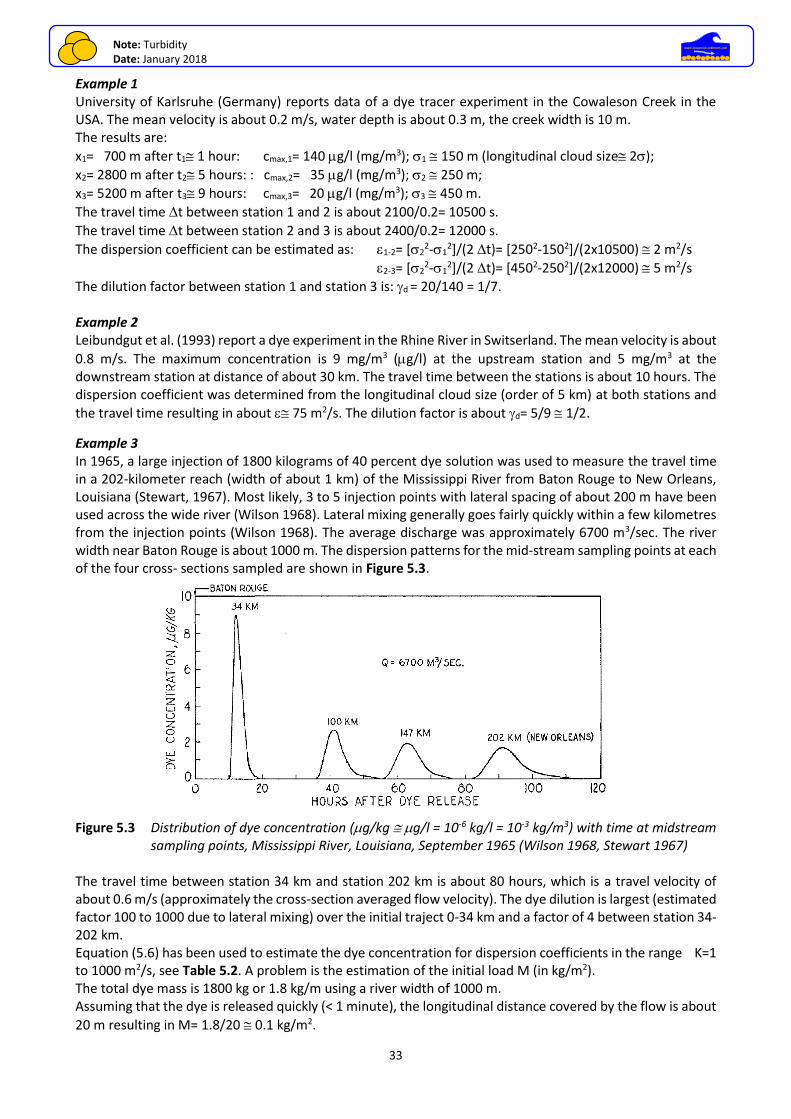
Note: Turbidity Date: January 2018
33
www.leovanrijn-sediment.com
Example 1 University of Karlsruhe (Germany) reports data of a dye tracer experiment in the Cowaleson Creek in the USA. The mean velocity is about 0.2 m/s, water depth is about 0.3 m, the creek width is 10 m. The results are:
x1= 700 m after t1 1 hour: cmax,1= 140 g/l (mg/m3); 1 150 m (longitudinal cloud size 2);
x2= 2800 m after t2 5 hours: : cmax,2= 35 g/l (mg/m3); 2 250 m;
x3= 5200 m after t3 9 hours: cmax,3= 20 g/l (mg/m3); 3 450 m.
The travel time t between station 1 and 2 is about 2100/0.2= 10500 s.
The travel time t between station 2 and 3 is about 2400/0.2= 12000 s.
The dispersion coefficient can be estimated as: 1-2= [22-1
2]/(2 t)= [2502-1502]/(2x10500) 2 m2/s
2-3= [22-1
2]/(2 t)= [4502-2502]/(2x12000) 5 m2/s
The dilution factor between station 1 and station 3 is: d = 20/140 = 1/7. Example 2 Leibundgut et al. (1993) report a dye experiment in the Rhine River in Switserland. The mean velocity is about
0.8 m/s. The maximum concentration is 9 mg/m3 (g/l) at the upstream station and 5 mg/m3 at the downstream station at distance of about 30 km. The travel time between the stations is about 10 hours. The dispersion coefficient was determined from the longitudinal cloud size (order of 5 km) at both stations and
the travel time resulting in about 75 m2/s. The dilution factor is about d= 5/9 1/2.
Example 3 In 1965, a large injection of 1800 kilograms of 40 percent dye solution was used to measure the travel time in a 202-kilometer reach (width of about 1 km) of the Mississippi River from Baton Rouge to New Orleans, Louisiana (Stewart, 1967). Most likely, 3 to 5 injection points with lateral spacing of about 200 m have been used across the wide river (Wilson 1968). Lateral mixing generally goes fairly quickly within a few kilometres from the injection points (Wilson 1968). The average discharge was approximately 6700 m3/sec. The river width near Baton Rouge is about 1000 m. The dispersion patterns for the mid-stream sampling points at each of the four cross- sections sampled are shown in Figure 5.3.
Figure 5.3 Distribution of dye concentration (g/kg g/l = 10-6 kg/l = 10-3 kg/m3) with time at midstream
sampling points, Mississippi River, Louisiana, September 1965 (Wilson 1968, Stewart 1967) The travel time between station 34 km and station 202 km is about 80 hours, which is a travel velocity of about 0.6 m/s (approximately the cross-section averaged flow velocity). The dye dilution is largest (estimated factor 100 to 1000 due to lateral mixing) over the initial traject 0-34 km and a factor of 4 between station 34-202 km. Equation (5.6) has been used to estimate the dye concentration for dispersion coefficients in the range K=1 to 1000 m2/s, see Table 5.2. A problem is the estimation of the initial load M (in kg/m2). The total dye mass is 1800 kg or 1.8 kg/m using a river width of 1000 m. Assuming that the dye is released quickly (< 1 minute), the longitudinal distance covered by the flow is about
20 m resulting in M= 1.8/20 0.1 kg/m2.
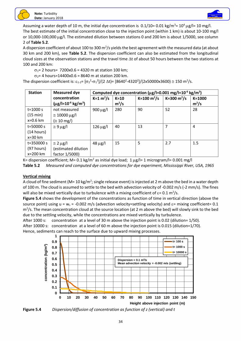
Note: Turbidity Date: January 2018
34
www.leovanrijn-sediment.com
Assuming a water depth of 10 m, the initial dye concentration is 0.1/10= 0.01 kg/m3= 104 g/l= 10 mg/l. The best estimate of the initial concentration close to the injection point (within 1 km) is about 10-100 mg/l
or 10,000-100,000 g/l. The estimated dilution between stations 0 and 200 km is about 1/5000, see column 2 of Table 5.2. A dispersion coefficient of about 100 to 300 m2/s yields the best agreement with the measured data (at about 30 km and 200 km), see Table 5.2. The dispersion coefficient can also be estimated from the longitudinal
cloud sizes at the observation stations and the travel time t of about 50 hours between the two stations at 100 and 200 km:
1= 2 hours= 7200x0.6 = 4320 m at station 100 km;
2= 4 hours=14400x0.6 = 8640 m at station 200 km.
The dispersion coefficient is: 1-2= [22-1
2]/(2 t)= [86402-43202]/(2x50000x3600) 150 m2/s.
Station Measured dye concentration
(g/l=10-6 kg/m3)
Computed dye concentration (g/l=0.001 mg/l=10-6 kg/m3)
K=1 m2/s K=10 m2/s
K=100 m2/s K=300 m2/s K=1000 m2/s
t=1000 s (15 min) x=0.6 km
not measured
10000 g/l
( 10 mg/)
900 g/l
280 90 52 28
t=50000 s (14 hours) x=30 km
9 g/l
126 g/l
40 13 7 4
t=350000 s (97 hours) x=200 km
2 g/l (estimated dilution factor 1/5000)
48 g/l
15 5 2.7 1.5
K= dispersion coefficient; M= 0.1 kg/m2 as initial dye load; 1 g/l= 1 microgram/l= 0.001 mg/l Table 5.2 Measured and computed dye concentrations for dye experiment, Mississippi River, USA, 1965 Vertical mixing A cloud of fine sediment (M= 10 kg/m2; single release event) is injected at 2 m above the bed in a water depth of 100 m. The cloud is assumed to settle to the bed with advection velocity of -0.002 m/s (-2 mm/s). The fines
will also be mixed vertically due to turbulence with a mixing coefficient of = 0.1 m2/s. Figure 5.4 shows the development of the concentrations as function of time in vertical direction (above the
source point) using u = ws = -0.002 m/s (advection velocity=settling velocity) and = mixing coefficient= 0.1 m2/s. The mean concentration cloud at the source location (at 2 m above the bed) will slowly sink to the bed due to the settling velocity, while the concentrations are mixed vertically by turbulence. After 1000 s: concentration at a level of 30 m above the injection point is 0.02 (dilution= 1/50). After 10000 s: concentration at a level of 60 m above the injection point is 0.015 (dilution=1/70). Hence, sediments can reach to the surface due to upward mixing processes.
Figure 5.4 Dispersion/diffusion of concentration as function of z (vertical) and t
0
0.1
0.2
0.3
0.4
0.5
0.6
0.7
0.8
0.9
1
0 10 20 30 40 50 60 70 80 90 100 110 120 130 140 150
co
ncen
trati
on
(kg
/m3)
Height above injection point (m)
t= 100 s
t= 1000 s
t= 10000 s
Dispersion = 0.1 m2/s Mean advection velocity = -0.002 m/s (settling)
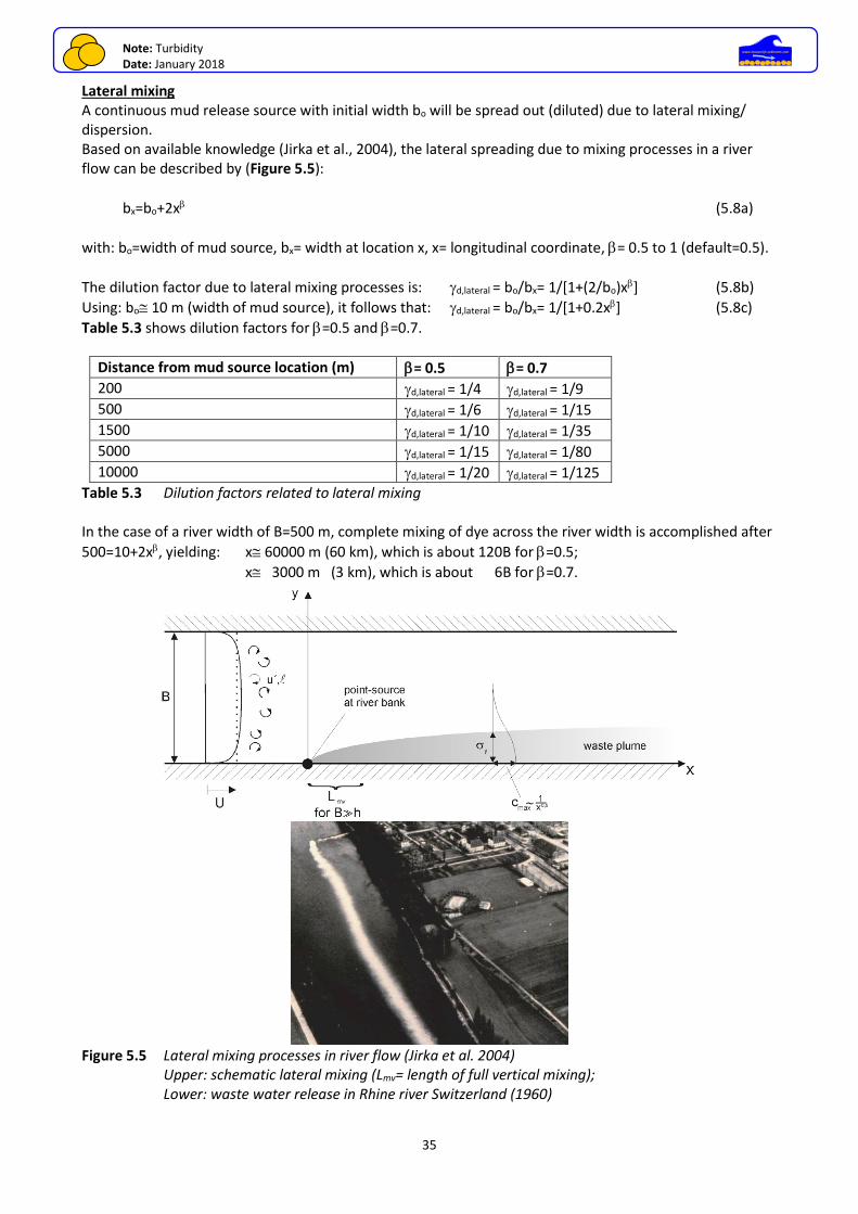
Note: Turbidity Date: January 2018
35
www.leovanrijn-sediment.com
Lateral mixing A continuous mud release source with initial width bo will be spread out (diluted) due to lateral mixing/ dispersion. Based on available knowledge (Jirka et al., 2004), the lateral spreading due to mixing processes in a river flow can be described by (Figure 5.5):
bx=bo+2x (5.8a)
with: bo=width of mud source, bx= width at location x, x= longitudinal coordinate, = 0.5 to 1 (default=0.5).
The dilution factor due to lateral mixing processes is: d,lateral = bo/bx= 1/[1+(2/bo)x] (5.8b)
Using: bo 10 m (width of mud source), it follows that: d,lateral = bo/bx= 1/[1+0.2x] (5.8c)
Table 5.3 shows dilution factors for =0.5 and =0.7.
Distance from mud source location (m) = 0.5 = 0.7
200 d,lateral = 1/4 d,lateral = 1/9
500 d,lateral = 1/6 d,lateral = 1/15
1500 d,lateral = 1/10 d,lateral = 1/35
5000 d,lateral = 1/15 d,lateral = 1/80
10000 d,lateral = 1/20 d,lateral = 1/125
Table 5.3 Dilution factors related to lateral mixing In the case of a river width of B=500 m, complete mixing of dye across the river width is accomplished after
500=10+2x, yielding: x 60000 m (60 km), which is about 120B for =0.5;
x 3000 m (3 km), which is about 6B for =0.7.
Figure 5.5 Lateral mixing processes in river flow (Jirka et al. 2004) Upper: schematic lateral mixing (Lmv= length of full vertical mixing); Lower: waste water release in Rhine river Switzerland (1960)
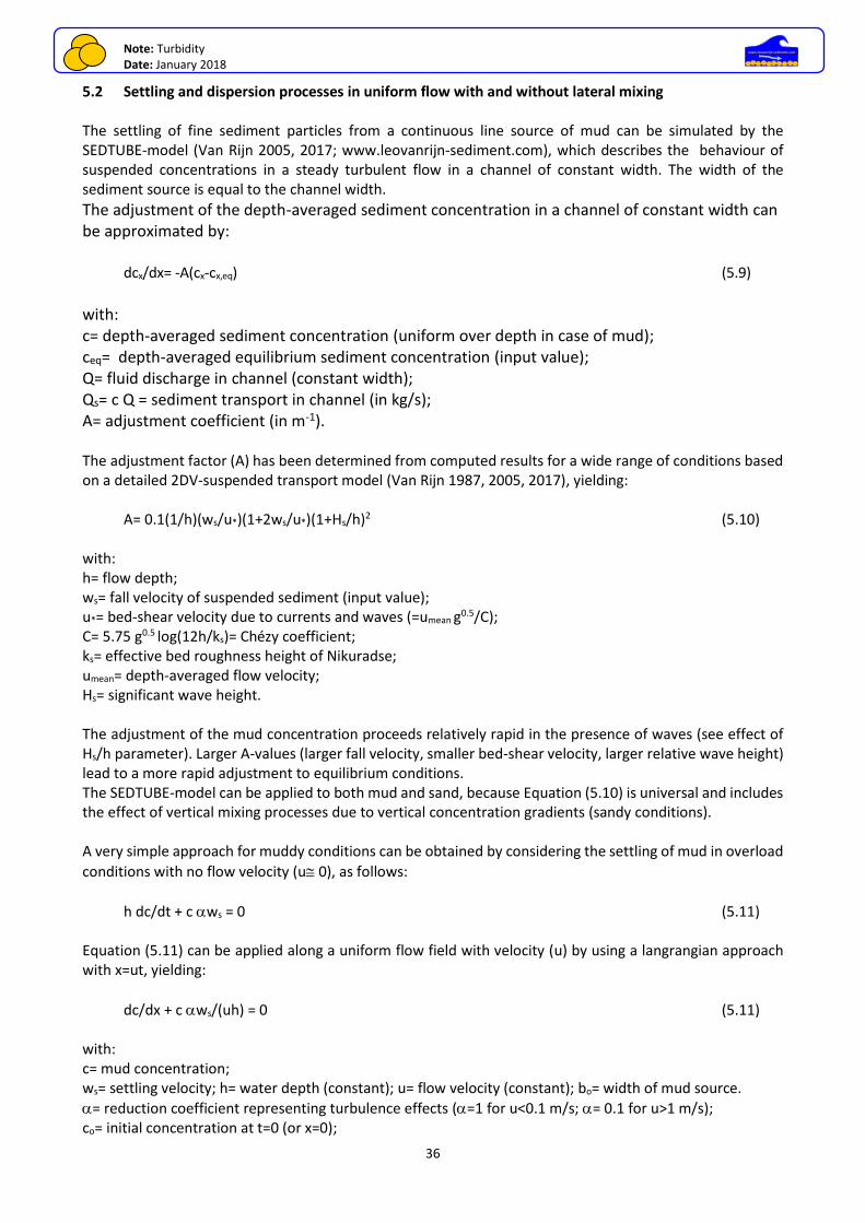
Note: Turbidity Date: January 2018
36
www.leovanrijn-sediment.com
5.2 Settling and dispersion processes in uniform flow with and without lateral mixing The settling of fine sediment particles from a continuous line source of mud can be simulated by the SEDTUBE-model (Van Rijn 2005, 2017; www.leovanrijn-sediment.com), which describes the behaviour of suspended concentrations in a steady turbulent flow in a channel of constant width. The width of the sediment source is equal to the channel width.
The adjustment of the depth-averaged sediment concentration in a channel of constant width can be approximated by: dcx/dx= -A(cx-cx,eq) (5.9)
with: c= depth-averaged sediment concentration (uniform over depth in case of mud); ceq= depth-averaged equilibrium sediment concentration (input value); Q= fluid discharge in channel (constant width); Qs= c Q = sediment transport in channel (in kg/s); A= adjustment coefficient (in m-1). The adjustment factor (A) has been determined from computed results for a wide range of conditions based on a detailed 2DV-suspended transport model (Van Rijn 1987, 2005, 2017), yielding: A= 0.1(1/h)(ws/u*)(1+2ws/u*)(1+Hs/h)2 (5.10) with: h= flow depth; ws= fall velocity of suspended sediment (input value); u*= bed-shear velocity due to currents and waves (=umean g0.5/C); C= 5.75 g0.5 log(12h/ks)= Chézy coefficient; ks= effective bed roughness height of Nikuradse; umean= depth-averaged flow velocity; Hs= significant wave height. The adjustment of the mud concentration proceeds relatively rapid in the presence of waves (see effect of Hs/h parameter). Larger A-values (larger fall velocity, smaller bed-shear velocity, larger relative wave height) lead to a more rapid adjustment to equilibrium conditions. The SEDTUBE-model can be applied to both mud and sand, because Equation (5.10) is universal and includes the effect of vertical mixing processes due to vertical concentration gradients (sandy conditions). A very simple approach for muddy conditions can be obtained by considering the settling of mud in overload
conditions with no flow velocity (u 0), as follows:
h dc/dt + c ws = 0 (5.11) Equation (5.11) can be applied along a uniform flow field with velocity (u) by using a langrangian approach with x=ut, yielding:
dc/dx + c ws/(uh) = 0 (5.11) with: c= mud concentration; ws= settling velocity; h= water depth (constant); u= flow velocity (constant); bo= width of mud source.
= reduction coefficient representing turbulence effects (=1 for u<0.1 m/s; = 0.1 for u>1 m/s); co= initial concentration at t=0 (or x=0);
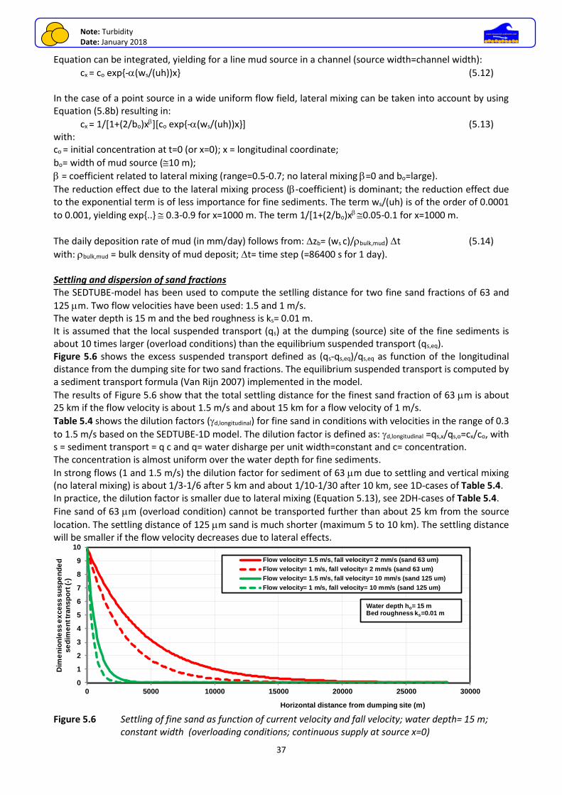
Note: Turbidity Date: January 2018
37
www.leovanrijn-sediment.com
Equation can be integrated, yielding for a line mud source in a channel (source width=channel width):
cx = co exp{-(ws/(uh))x} (5.12) In the case of a point source in a wide uniform flow field, lateral mixing can be taken into account by using Equation (5.8b) resulting in:
cx = 1/[1+(2/bo)x][co exp{-(ws/(uh))x}] (5.13) with: co = initial concentration at t=0 (or x=0); x = longitudinal coordinate;
bo= width of mud source (10 m);
= coefficient related to lateral mixing (range=0.5-0.7; no lateral mixing =0 and bo=large).
The reduction effect due to the lateral mixing process (-coefficient) is dominant; the reduction effect due to the exponential term is of less importance for fine sediments. The term ws/(uh) is of the order of 0.0001
to 0.001, yielding exp{..} 0.3-0.9 for x=1000 m. The term 1/[1+(2/bo)x 0.05-0.1 for x=1000 m.
The daily deposition rate of mud (in mm/day) follows from: zb= (ws c)/bulk,mud) t (5.14)
with: bulk,mud = bulk density of mud deposit; t= time step (=86400 s for 1 day). Settling and dispersion of sand fractions The SEDTUBE-model has been used to compute the setlling distance for two fine sand fractions of 63 and
125 m. Two flow velocities have been used: 1.5 and 1 m/s. The water depth is 15 m and the bed roughness is ks= 0.01 m. It is assumed that the local suspended transport (qs) at the dumping (source) site of the fine sediments is about 10 times larger (overload conditions) than the equilibrium suspended transport (qs,eq). Figure 5.6 shows the excess suspended transport defined as (qs-qs,eq)/qs,eq as function of the longitudinal distance from the dumping site for two sand fractions. The equilibrium suspended transport is computed by a sediment transport formula (Van Rijn 2007) implemented in the model.
The results of Figure 5.6 show that the total settling distance for the finest sand fraction of 63 m is about 25 km if the flow velocity is about 1.5 m/s and about 15 km for a flow velocity of 1 m/s.
Table 5.4 shows the dilution factors (d,longitudinal) for fine sand in conditions with velocities in the range of 0.3
to 1.5 m/s based on the SEDTUBE-1D model. The dilution factor is defined as: d,longitudinal =qs,x/qs,o=cx/co, with s = sediment transport = q c and q= water disharge per unit width=constant and c= concentration. The concentration is almost uniform over the water depth for fine sediments.
In strong flows (1 and 1.5 m/s) the dilution factor for sediment of 63 m due to settling and vertical mixing (no lateral mixing) is about 1/3-1/6 after 5 km and about 1/10-1/30 after 10 km, see 1D-cases of Table 5.4. In practice, the dilution factor is smaller due to lateral mixing (Equation 5.13), see 2DH-cases of Table 5.4.
Fine sand of 63 m (overload condition) cannot be transported further than about 25 km from the source
location. The settling distance of 125 m sand is much shorter (maximum 5 to 10 km). The settling distance will be smaller if the flow velocity decreases due to lateral effects.
Figure 5.6 Settling of fine sand as function of current velocity and fall velocity; water depth= 15 m; constant width (overloading conditions; continuous supply at source x=0)
0
1
2
3
4
5
6
7
8
9
10
0 5000 10000 15000 20000 25000 30000
Dim
en
ion
less e
xcess s
usp
en
de
d
se
dim
en
t tr
an
sp
ort
(-)
Horizontal distance from dumping site (m)
Flow velocity= 1.5 m/s, fall velocity= 2 mm/s (sand 63 um)
Flow velocity= 1 m/s, fall velocity= 2 mm/s (sand 63 um)
Flow velocity= 1.5 m/s, fall velocity= 10 mm/s (sand 125 um)
Flow velocity= 1 m/s, fall velocity= 10 mm/s (sand 125 um)
Water depth ho= 15 m Bed roughness ks=0.01 m
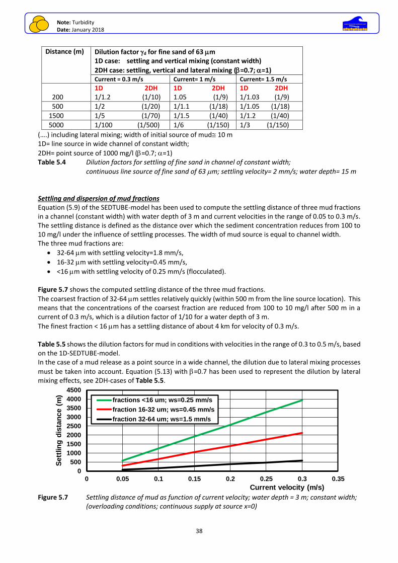
Note: Turbidity Date: January 2018
38
www.leovanrijn-sediment.com
Distance (m) Dilution factor d for fine sand of 63 m 1D case: settling and vertical mixing (constant width)
2DH case: settling, vertical and lateral mixing (=0.7; =1) Current = 0.3 m/s Current= 1 m/s Current= 1.5 m/s
200
1D 2DH 1/1.2 (1/10)
1D 2DH 1.05 (1/9)
1D 2DH 1/1.03 (1/9)
500 1/2 (1/20) 1/1.1 (1/18) 1/1.05 (1/18)
1500 1/5 (1/70) 1/1.5 (1/40) 1/1.2 (1/40)
5000 1/100 (1/500) 1/6 (1/150) 1/3 (1/150)
(….) including lateral mixing; width of initial source of mud 10 m 1D= line source in wide channel of constant width;
2DH= point source of 1000 mg/l (=0.7; =1) Table 5.4 Dilution factors for settling of fine sand in channel of constant width;
continuous line source of fine sand of 63 m; settling velocity= 2 mm/s; water depth= 15 m Settling and dispersion of mud fractions Equation (5.9) of the SEDTUBE-model has been used to compute the settling distance of three mud fractions in a channel (constant width) with water depth of 3 m and current velocities in the range of 0.05 to 0.3 m/s. The settling distance is defined as the distance over which the sediment concentration reduces from 100 to 10 mg/l under the influence of settling processes. The width of mud source is equal to channel width. The three mud fractions are:
• 32-64 m with settling velocity=1.8 mm/s,
• 16-32 m with settling velocity=0.45 mm/s,
• <16 m with settling velocity of 0.25 mm/s (flocculated). Figure 5.7 shows the computed settling distance of the three mud fractions.
The coarsest fraction of 32-64 m settles relatively quickly (within 500 m from the line source location). This means that the concentrations of the coarsest fraction are reduced from 100 to 10 mg/l after 500 m in a current of 0.3 m/s, which is a dilution factor of 1/10 for a water depth of 3 m.
The finest fraction < 16 m has a settling distance of about 4 km for velocity of 0.3 m/s. Table 5.5 shows the dilution factors for mud in conditions with velocities in the range of 0.3 to 0.5 m/s, based on the 1D-SEDTUBE-model. In the case of a mud release as a point source in a wide channel, the dilution due to lateral mixing processes
must be taken into account. Equation (5.13) with =0.7 has been used to represent the dilution by lateral mixing effects, see 2DH-cases of Table 5.5.
Figure 5.7 Settling distance of mud as function of current velocity; water depth = 3 m; constant width; (overloading conditions; continuous supply at source x=0)
0
500
1000
1500
2000
2500
3000
3500
4000
4500
0 0.05 0.1 0.15 0.2 0.25 0.3 0.35
Sett
lin
g d
ista
nce (
m)
Current velocity (m/s)
fractions <16 um; ws=0.25 mm/s
fraction 16-32 um; ws=0.45 mm/s
fraction 32-64 um; ws=1.5 mm/s
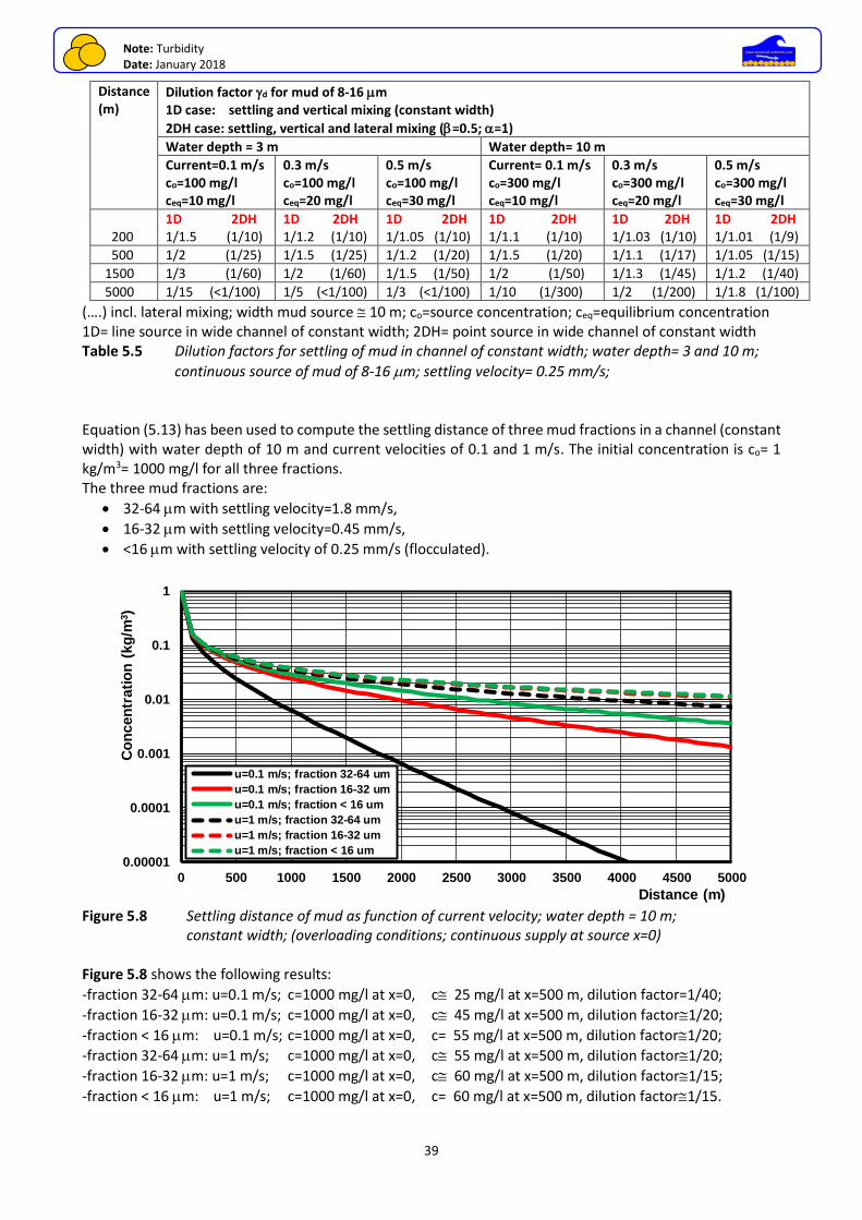
Note: Turbidity Date: January 2018
39
www.leovanrijn-sediment.com
Distance (m)
Dilution factor d for mud of 8-16 m 1D case: settling and vertical mixing (constant width)
2DH case: settling, vertical and lateral mixing (=0.5; =1)
Water depth = 3 m Water depth= 10 m
Current=0.1 m/s co=100 mg/l ceq=10 mg/l
0.3 m/s co=100 mg/l ceq=20 mg/l
0.5 m/s co=100 mg/l ceq=30 mg/l
Current= 0.1 m/s co=300 mg/l ceq=10 mg/l
0.3 m/s co=300 mg/l ceq=20 mg/l
0.5 m/s co=300 mg/l ceq=30 mg/l
200
1D 2DH 1/1.5 (1/10)
1D 2DH 1/1.2 (1/10)
1D 2DH 1/1.05 (1/10)
1D 2DH 1/1.1 (1/10)
1D 2DH 1/1.03 (1/10)
1D 2DH 1/1.01 (1/9)
500 1/2 (1/25) 1/1.5 (1/25) 1/1.2 (1/20) 1/1.5 (1/20) 1/1.1 (1/17) 1/1.05 (1/15)
1500 1/3 (1/60) 1/2 (1/60) 1/1.5 (1/50) 1/2 (1/50) 1/1.3 (1/45) 1/1.2 (1/40)
5000 1/15 (<1/100) 1/5 (<1/100) 1/3 (<1/100) 1/10 (1/300) 1/2 (1/200) 1/1.8 (1/100)
(….) incl. lateral mixing; width mud source 10 m; co=source concentration; ceq=equilibrium concentration 1D= line source in wide channel of constant width; 2DH= point source in wide channel of constant width Table 5.5 Dilution factors for settling of mud in channel of constant width; water depth= 3 and 10 m;
continuous source of mud of 8-16 m; settling velocity= 0.25 mm/s; Equation (5.13) has been used to compute the settling distance of three mud fractions in a channel (constant width) with water depth of 10 m and current velocities of 0.1 and 1 m/s. The initial concentration is co= 1 kg/m3= 1000 mg/l for all three fractions. The three mud fractions are:
• 32-64 m with settling velocity=1.8 mm/s,
• 16-32 m with settling velocity=0.45 mm/s,
• <16 m with settling velocity of 0.25 mm/s (flocculated).
Figure 5.8 Settling distance of mud as function of current velocity; water depth = 10 m; constant width; (overloading conditions; continuous supply at source x=0) Figure 5.8 shows the following results:
-fraction 32-64 m: u=0.1 m/s; c=1000 mg/l at x=0, c 25 mg/l at x=500 m, dilution factor=1/40;
-fraction 16-32 m: u=0.1 m/s; c=1000 mg/l at x=0, c 45 mg/l at x=500 m, dilution factor1/20;
-fraction < 16 m: u=0.1 m/s; c=1000 mg/l at x=0, c= 55 mg/l at x=500 m, dilution factor1/20;
-fraction 32-64 m: u=1 m/s; c=1000 mg/l at x=0, c 55 mg/l at x=500 m, dilution factor1/20;
-fraction 16-32 m: u=1 m/s; c=1000 mg/l at x=0, c 60 mg/l at x=500 m, dilution factor1/15;
-fraction < 16 m: u=1 m/s; c=1000 mg/l at x=0, c= 60 mg/l at x=500 m, dilution factor1/15.
0.00001
0.0001
0.001
0.01
0.1
1
0 500 1000 1500 2000 2500 3000 3500 4000 4500 5000
Co
ncen
trati
on
(kg
/m3)
Distance (m)
u=0.1 m/s; fraction 32-64 um
u=0.1 m/s; fraction 16-32 um
u=0.1 m/s; fraction < 16 um
u=1 m/s; fraction 32-64 um
u=1 m/s; fraction 16-32 um
u=1 m/s; fraction < 16 um
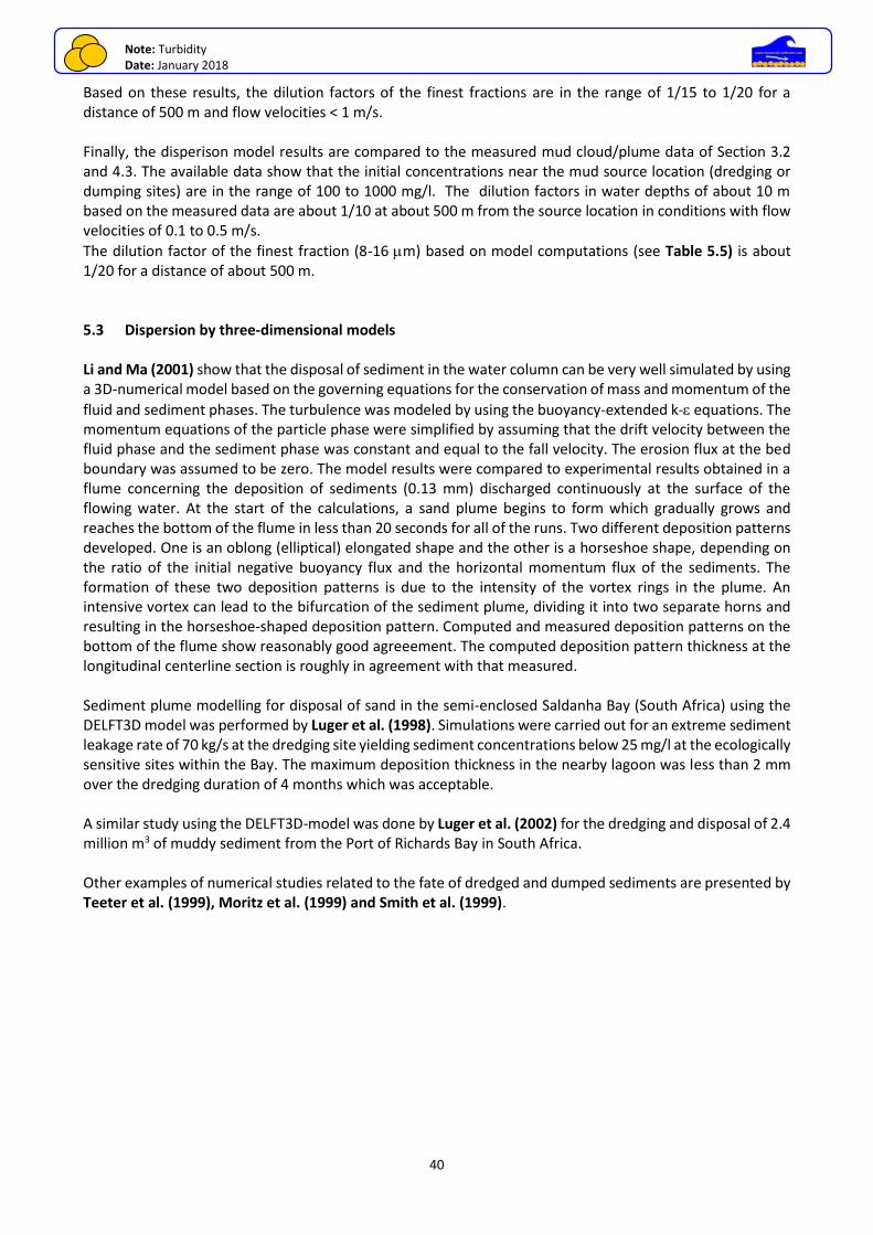
Note: Turbidity Date: January 2018
40
www.leovanrijn-sediment.com
Based on these results, the dilution factors of the finest fractions are in the range of 1/15 to 1/20 for a distance of 500 m and flow velocities < 1 m/s. Finally, the disperison model results are compared to the measured mud cloud/plume data of Section 3.2 and 4.3. The available data show that the initial concentrations near the mud source location (dredging or dumping sites) are in the range of 100 to 1000 mg/l. The dilution factors in water depths of about 10 m based on the measured data are about 1/10 at about 500 m from the source location in conditions with flow velocities of 0.1 to 0.5 m/s.
The dilution factor of the finest fraction (8-16 m) based on model computations (see Table 5.5) is about 1/20 for a distance of about 500 m. 5.3 Dispersion by three-dimensional models Li and Ma (2001) show that the disposal of sediment in the water column can be very well simulated by using a 3D-numerical model based on the governing equations for the conservation of mass and momentum of the
fluid and sediment phases. The turbulence was modeled by using the buoyancy-extended k- equations. The momentum equations of the particle phase were simplified by assuming that the drift velocity between the fluid phase and the sediment phase was constant and equal to the fall velocity. The erosion flux at the bed boundary was assumed to be zero. The model results were compared to experimental results obtained in a flume concerning the deposition of sediments (0.13 mm) discharged continuously at the surface of the flowing water. At the start of the calculations, a sand plume begins to form which gradually grows and reaches the bottom of the flume in less than 20 seconds for all of the runs. Two different deposition patterns developed. One is an oblong (elliptical) elongated shape and the other is a horseshoe shape, depending on the ratio of the initial negative buoyancy flux and the horizontal momentum flux of the sediments. The formation of these two deposition patterns is due to the intensity of the vortex rings in the plume. An intensive vortex can lead to the bifurcation of the sediment plume, dividing it into two separate horns and resulting in the horseshoe-shaped deposition pattern. Computed and measured deposition patterns on the bottom of the flume show reasonably good agreeement. The computed deposition pattern thickness at the longitudinal centerline section is roughly in agreement with that measured. Sediment plume modelling for disposal of sand in the semi-enclosed Saldanha Bay (South Africa) using the DELFT3D model was performed by Luger et al. (1998). Simulations were carried out for an extreme sediment leakage rate of 70 kg/s at the dredging site yielding sediment concentrations below 25 mg/l at the ecologically sensitive sites within the Bay. The maximum deposition thickness in the nearby lagoon was less than 2 mm over the dredging duration of 4 months which was acceptable. A similar study using the DELFT3D-model was done by Luger et al. (2002) for the dredging and disposal of 2.4 million m3 of muddy sediment from the Port of Richards Bay in South Africa. Other examples of numerical studies related to the fate of dredged and dumped sediments are presented by Teeter et al. (1999), Moritz et al. (1999) and Smith et al. (1999).
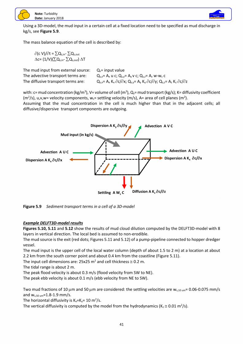
Note: Turbidity Date: January 2018
41
www.leovanrijn-sediment.com
Using a 3D-model, the mud input in a certain cell at a fixed location need to be specified as mud discharge in kg/s, see Figure 5.9. The mass balance equation of the cell is described by:
(c V)/t = Qs,in- Qs,out
c= (1/V)(Qs,in- Qs,out) T The mud input from external source: Qs= input value The advective transport terms are: Qs,x= Ax u c; Qs,y= Ay v c; Qs,z= Az w-ws c
The diffusive transport terms are: Qs,x= Ax Kx c/x; Qs,y= Ay Ky c/y; Qs,z= Az Kz c/z with: c= mud concentration (kg/m3), V= volume of cell (m3), Qs= mud transport (kg/s); K= diffusivity coefficient (m2/s), u,v,w= velocity components, ws= settling velocity (m/s), A= area of cell planes (m2). Assuming that the mud concentration in the cell is much higher than that in the adjacent cells; all diffusive/dispersive transport components are outgoing.
Figure 5.9 Sediment transport terms in a cell of a 3D-model Example DELFT3D-model results Figures 5.10, 5.11 and 5.12 show the results of mud cloud dilution computed by the DELFT3D-model with 8 layers in vertical direction. The local bed is assumed to non-erodible. The mud source is the exit (red dots; Figures 5.11 and 5.12) of a pump-pipeline connected to hopper dredger vessel. The mud input is the upper cell of the local water column (depth of about 1.5 to 2 m) at a location at about 2.2 km from the south corner point and about 0.4 km from the coastline (Figure 5.11).
The input cell dimensions are: 25x25 m2 and cell thickness 0.2 m. The tidal range is about 2 m. The peak flood velocity is about 0.3 m/s (flood velocity from SW to NE). The peak ebb velocity is about 0.1 m/s (ebb velocity from NE to SW).
Two mud fractions of 10 m and 50 m are considered: the settling velocities are ws,10 um= 0.06-0.075 mm/s and ws,50 um=1.8-1.9 mm/s. The horizontal diffusivity is Kx=Ky= 10 m2/s.
The vertical diffusivity is computed by the model from the hydrodynamics (Kz 0.01 m2/s).
Advection A U C
Dispersion A Kx c/x
Advection A U C
Dispersion A Kx c/x
Dispersion A Ky c/y Advection A V C
Settling A Ws C Diffusion A Kz c/z
Mud input (in kg/s)
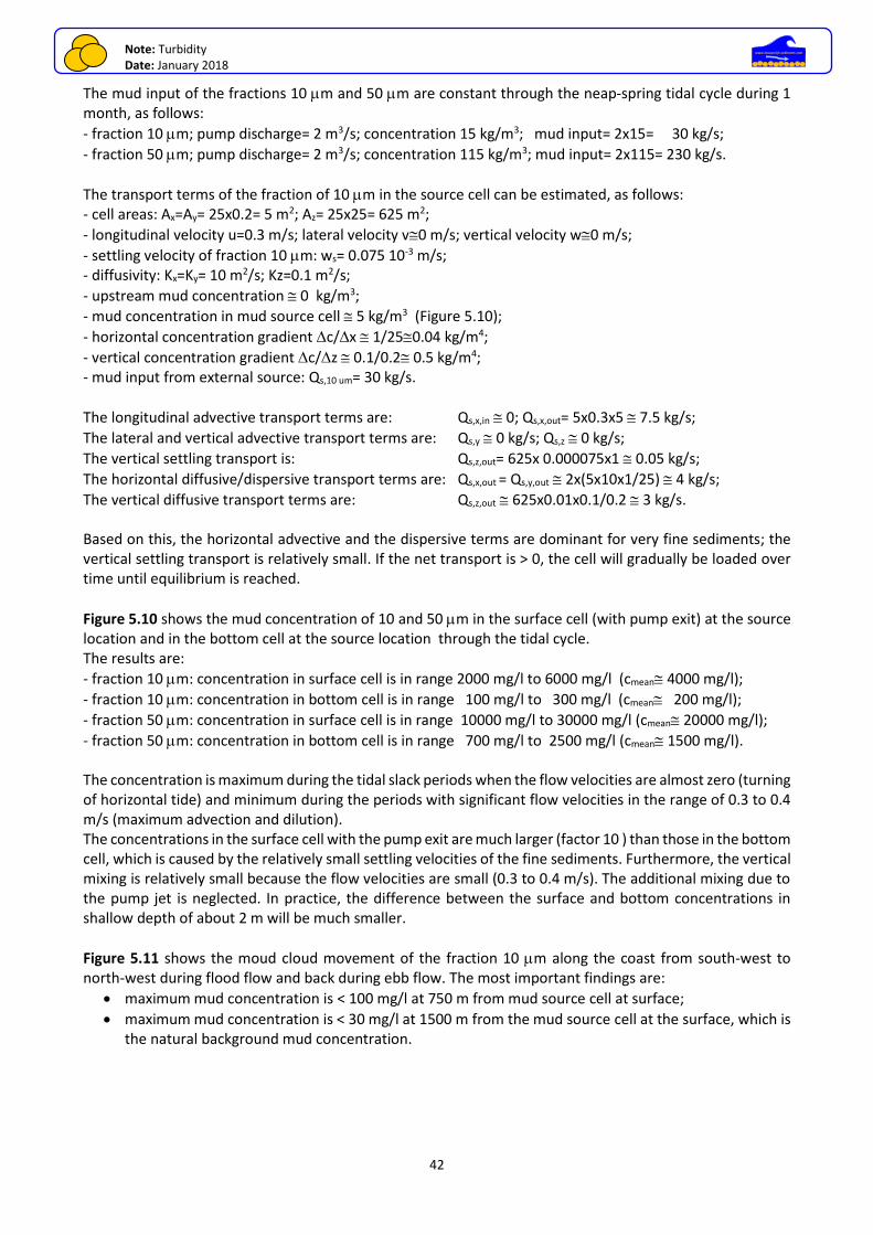
Note: Turbidity Date: January 2018
42
www.leovanrijn-sediment.com
The mud input of the fractions 10 m and 50 m are constant through the neap-spring tidal cycle during 1 month, as follows:
- fraction 10 m; pump discharge= 2 m3/s; concentration 15 kg/m3; mud input= 2x15= 30 kg/s;
- fraction 50 m; pump discharge= 2 m3/s; concentration 115 kg/m3; mud input= 2x115= 230 kg/s.
The transport terms of the fraction of 10 m in the source cell can be estimated, as follows: - cell areas: Ax=Ay= 25x0.2= 5 m2; Az= 25x25= 625 m2;
- longitudinal velocity u=0.3 m/s; lateral velocity v0 m/s; vertical velocity w0 m/s;
- settling velocity of fraction 10 m: ws= 0.075 10-3 m/s; - diffusivity: Kx=Ky= 10 m2/s; Kz=0.1 m2/s;
- upstream mud concentration 0 kg/m3;
- mud concentration in mud source cell 5 kg/m3 (Figure 5.10);
- horizontal concentration gradient c/x 1/250.04 kg/m4;
- vertical concentration gradient c/z 0.1/0.2 0.5 kg/m4; - mud input from external source: Qs,10 um= 30 kg/s.
The longitudinal advective transport terms are: Qs,x,in 0; Qs,x,out= 5x0.3x5 7.5 kg/s;
The lateral and vertical advective transport terms are: Qs,y 0 kg/s; Qs,z 0 kg/s;
The vertical settling transport is: Qs,z,out= 625x 0.000075x1 0.05 kg/s;
The horizontal diffusive/dispersive transport terms are: Qs,x,out = Qs,y,out 2x(5x10x1/25) 4 kg/s;
The vertical diffusive transport terms are: Qs,z,out 625x0.01x0.1/0.2 3 kg/s. Based on this, the horizontal advective and the dispersive terms are dominant for very fine sediments; the vertical settling transport is relatively small. If the net transport is > 0, the cell will gradually be loaded over time until equilibrium is reached.
Figure 5.10 shows the mud concentration of 10 and 50 m in the surface cell (with pump exit) at the source location and in the bottom cell at the source location through the tidal cycle. The results are:
- fraction 10 m: concentration in surface cell is in range 2000 mg/l to 6000 mg/l (cmean 4000 mg/l);
- fraction 10 m: concentration in bottom cell is in range 100 mg/l to 300 mg/l (cmean 200 mg/l);
- fraction 50 m: concentration in surface cell is in range 10000 mg/l to 30000 mg/l (cmean 20000 mg/l);
- fraction 50 m: concentration in bottom cell is in range 700 mg/l to 2500 mg/l (cmean 1500 mg/l). The concentration is maximum during the tidal slack periods when the flow velocities are almost zero (turning of horizontal tide) and minimum during the periods with significant flow velocities in the range of 0.3 to 0.4 m/s (maximum advection and dilution). The concentrations in the surface cell with the pump exit are much larger (factor 10 ) than those in the bottom cell, which is caused by the relatively small settling velocities of the fine sediments. Furthermore, the vertical mixing is relatively small because the flow velocities are small (0.3 to 0.4 m/s). The additional mixing due to the pump jet is neglected. In practice, the difference between the surface and bottom concentrations in shallow depth of about 2 m will be much smaller.
Figure 5.11 shows the moud cloud movement of the fraction 10 m along the coast from south-west to north-west during flood flow and back during ebb flow. The most important findings are:
• maximum mud concentration is < 100 mg/l at 750 m from mud source cell at surface;
• maximum mud concentration is < 30 mg/l at 1500 m from the mud source cell at the surface, which is the natural background mud concentration.
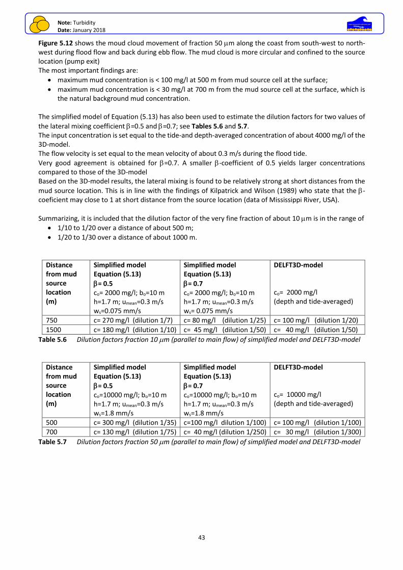
Note: Turbidity Date: January 2018
43
www.leovanrijn-sediment.com
Figure 5.12 shows the moud cloud movement of fraction 50 m along the coast from south-west to north-west during flood flow and back during ebb flow. The mud cloud is more circular and confined to the source location (pump exit) The most important findings are:
• maximum mud concentration is < 100 mg/l at 500 m from mud source cell at the surface;
• maximum mud concentration is < 30 mg/l at 700 m from the mud source cell at the surface, which is the natural background mud concentration.
The simplified model of Equation (5.13) has also been used to estimate the dilution factors for two values of
the lateral mixing coefficient =0.5 and =0.7; see Tables 5.6 and 5.7. The input concentration is set equal to the tide-and depth-averaged concentration of about 4000 mg/l of the 3D-model. The flow velocity is set equal to the mean velocity of about 0.3 m/s during the flood tide.
Very good agreement is obtained for =0.7. A smaller -coefficient of 0.5 yields larger concentrations compared to those of the 3D-model Based on the 3D-model results, the lateral mixing is found to be relatively strong at short distances from the
mud source location. This is in line with the findings of Kilpatrick and Wilson (1989) who state that the -coeficient may close to 1 at short distance from the source location (data of Mississippi River, USA).
Summarizing, it is included that the dilution factor of the very fine fraction of about 10 m is in the range of
• 1/10 to 1/20 over a distance of about 500 m;
• 1/20 to 1/30 over a distance of about 1000 m.
Distance from mud source location (m)
Simplified model Equation (5.13)
= 0.5 co= 2000 mg/l; bo=10 m h=1.7 m; umean=0.3 m/s ws=0.075 mm/s
Simplified model Equation (5.13)
= 0.7 co= 2000 mg/l; bo=10 m h=1.7 m; umean=0.3 m/s ws= 0.075 mm/s
DELFT3D-model co= 2000 mg/l (depth and tide-averaged)
750 c= 270 mg/l (dilution 1/7) c= 80 mg/l (dilution 1/25) c= 100 mg/l (dilution 1/20)
1500 c= 180 mg/l (dilution 1/10) c= 45 mg/l (dilution 1/50) c= 40 mg/l (dilution 1/50)
Table 5.6 Dilution factors fraction 10 m (parallel to main flow) of simplified model and DELFT3D-model
Distance from mud source location (m)
Simplified model Equation (5.13)
= 0.5 co=10000 mg/l; bo=10 m h=1.7 m; umean=0.3 m/s ws=1.8 mm/s
Simplified model Equation (5.13)
= 0.7 co=10000 mg/l; bo=10 m h=1.7 m; umean=0.3 m/s ws=1.8 mm/s
DELFT3D-model co= 10000 mg/l (depth and tide-averaged)
500 c= 300 mg/l (dilution 1/35) c=100 mg/l dilution 1/100) c= 100 mg/l (dilution 1/100)
700 c= 130 mg/l (dilution 1/75) c= 40 mg/l (dilution 1/250) c= 30 mg/l (dilution 1/300)
Table 5.7 Dilution factors fraction 50 m (parallel to main flow) of simplified model and DELFT3D-model
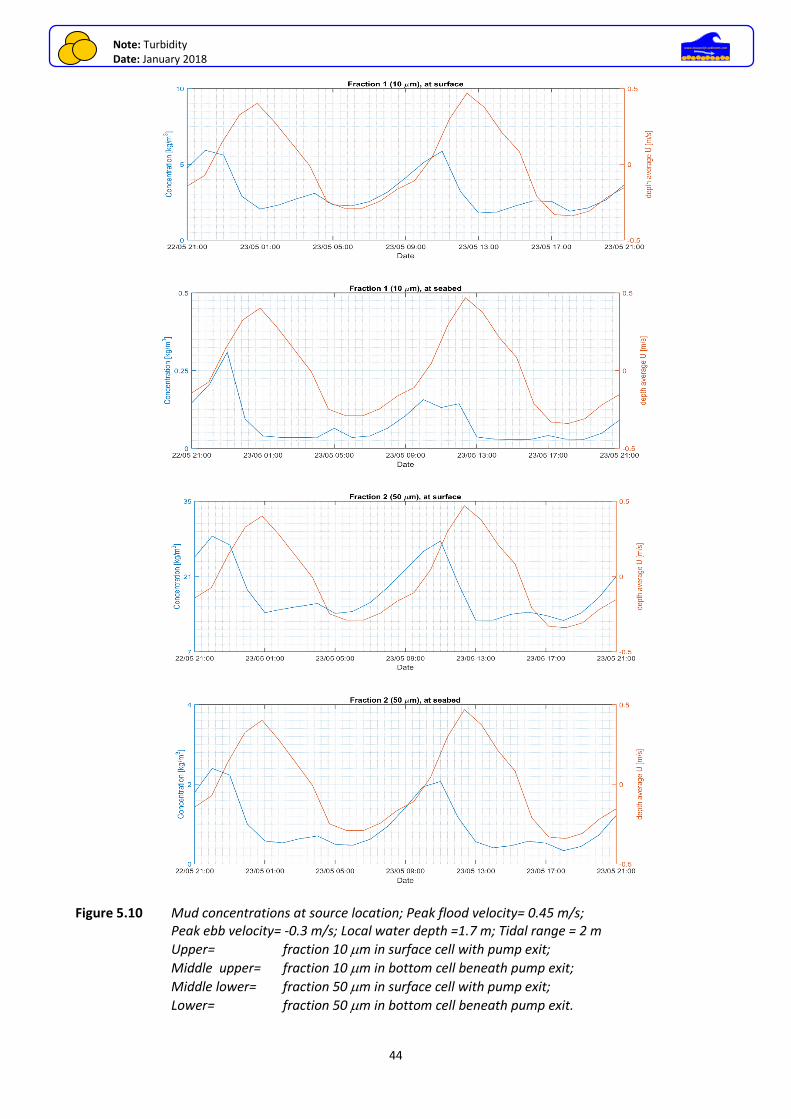
Note: Turbidity Date: January 2018
44
www.leovanrijn-sediment.com
Figure 5.10 Mud concentrations at source location; Peak flood velocity= 0.45 m/s;
Peak ebb velocity= -0.3 m/s; Local water depth =1.7 m; Tidal range = 2 m
Upper= fraction 10 m in surface cell with pump exit;
Middle upper= fraction 10 m in bottom cell beneath pump exit;
Middle lower= fraction 50 m in surface cell with pump exit;
Lower= fraction 50 m in bottom cell beneath pump exit.
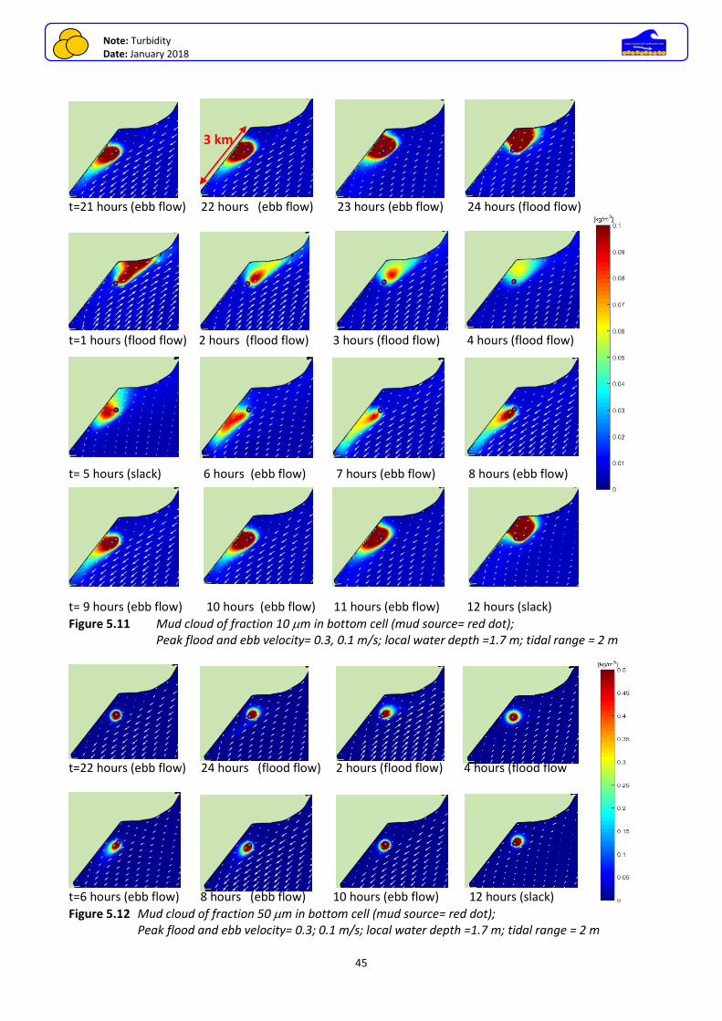
Note: Turbidity Date: January 2018
45
www.leovanrijn-sediment.com
t=21 hours (ebb flow) 22 hours (ebb flow) 23 hours (ebb flow) 24 hours (flood flow)
t=1 hours (flood flow) 2 hours (flood flow) 3 hours (flood flow) 4 hours (flood flow)
t= 5 hours (slack) 6 hours (ebb flow) 7 hours (ebb flow) 8 hours (ebb flow)
t= 9 hours (ebb flow) 10 hours (ebb flow) 11 hours (ebb flow) 12 hours (slack)
Figure 5.11 Mud cloud of fraction 10 m in bottom cell (mud source= red dot); Peak flood and ebb velocity= 0.3, 0.1 m/s; local water depth =1.7 m; tidal range = 2 m
t=22 hours (ebb flow) 24 hours (flood flow) 2 hours (flood flow) 4 hours (flood flow
t=6 hours (ebb flow) 8 hours (ebb flow) 10 hours (ebb flow) 12 hours (slack)
Figure 5.12 Mud cloud of fraction 50 m in bottom cell (mud source= red dot); Peak flood and ebb velocity= 0.3; 0.1 m/s; local water depth =1.7 m; tidal range = 2 m
3 km
Note: Turbidity Date: January 2018
46
www.leovanrijn-sediment.com
6. References Battisto, G.M. and Friedrichs, C.T., 2003. Monitoring suspended sediment plume formed during dredging
using ADCP, OBS and bottle samples. Coastal Sediments, Florida, USA Bernard, W.D., 1978. Prediction and control of dredged material dispersion around dredging and open-water
pipeline disposal operations. Technical Report DS-7-13, Dredged Material Research Program. USWES, Environmental Laboratory, Vicksburg, USA
Blokland, T., 1988. Determination of dredging-induced turbidity. Terra et Aqua, No. 38 Boot, M. 2000. Near-field dispersal of overflow loss of hopper dredger (in Dutch). MSc. Thesis, Civil
Engineering, Delft University of Technology Brouwer, J., Visser, K.G., Nelis, J.G. and Van Berk, H., 1991. Silt removal with Punaise, a flexible self-burying
dredging system. Paper E3, Proc. CEDA-PIANC Conference, Amsterdam, Netherlands Deltares, 1994. Density current analysis in the case of water injection dredging. Report J996. Delft, The
Netherlands Deltares, 1995. Demonstration tests water injection dredging (in Dutch). Report J1014. Delft, The Netherlands Hayes, D.F., Raymond, G.L. and Mc Lellan, T.N., 1984. Sediment resuspension from dredging activities, p. 72-
82. Dredging and dredged material disposal, Vol. I, ed. by R.L. Montgomery and J.W. Leach. Proc. of Conf. Dredging, Florida, USA
Healy, T., Ipenz, M. and Tian, F., 1999. Bypassing of dredged muddy sediment and thin layer disposal, Hauraki Gulf, New Zealand, p. 2457-2470. Coastal Sediments, Long Island, USA
Healy, T., Mehta, A., Rodriquez, H. and Tian, F., 1999. Bypassing of dredged littoral muddy sediments using a thin layer dispersal technique, p. 1119-1131. Journal of Coastal Research, Vol. 15, No. 4
Jirka, G.H. et al., 2004. Management of point source discharges into rivers. International Journal River Basin Management, Vol. 2, No. 3, 225-233.
Jobson, H.E., 1996. Prediction of travel time and longitudinal dispersion in rivers and streams. Publication USGS, USA
John, S.A. et al., 2000. Scoping the assessment of sediment plumes from dredging. CIRIA, London Kilpatrick, F.A. and Wilson, J.F., 1989. Measurements of time travel in streams by dye injection. Publication
USGS, USA Kirby, R. and Land, J.M., 1991. The impact of dredging: a comparison of natural and man-made disturbances
to cohesive sedimentary regimes. Paper B3, Proc. CEDA-PIANC Conference,Amsterdam, Netherlands LASC Task Force, 2003. Literature review of effects of resuspended sediments due to dredging operations.
Anchor Environmental CA, L.P. Irvine, California, USA Leibundgut, Ch., Speidel, U. and Wiesner,H., 1993. Transport processes in rivers investigated by tracer
experiments. Tracer Hydrology, IAHS publication No. 215 Li, C.W. and Ma, F.X., 2001. 3D numerical simulation of deposition patterns due to sand disposal in flowing
water, p. 209-218. Journal of Hydraulic Engineering, Vol. 127, No. 3 Luger, S.A., Schoonees, J.S., Mocke, G.P. and Smit, F., 1998. Predicting and evaluating turbidity caused by
dredging in the environmentally sensitive Saldanha Bay, p. 3561-3575. 26th ICCE, Copenhagen, Denmark
Luger, S.A., Schoonees, J.S. and Theron, A., 2002. Optimising the disposal of dredge spoil using numerical modelling, p. 3155-3167. 28th ICCE, Cardiff, UK
Mastbergen, D.R. and Van den Berg, J.H., 2003. Breaching in fine sands and the generation of sustained turbidity currents in submarine canyons. Sedimentology, Vol. 50, 625-637
Meulblok, M. en Van Weezenbeek, R.N., 1986. Water injection dredging In Dutch). De Ingenieur No. 10, The Netherlands
Meyvis, L., Stordiau, M. and Marsain, J., 1987. Maintenance dredging in tidal inlets, lock entrances and estuaries with alternative, low cost equipment, p. 1435-1446. Coastal and Port Engineering, Vol. II, Beijing, China
Moritz, H.P., Kraus, N.C. and Siipola, M.D., 1999. Simulating the fate of dredged material, Columbia River, USA, p. 2487-2503. Coastal Sediments, Long Island, USA
Ning Chien, 1998. Mechanics of sediment transport. ASCE Press
Note: Turbidity Date: January 2018
47
www.leovanrijn-sediment.com
Parks, J., 1991. Removing shoals from small harbor entrances by fluidization. Paper E2, Proc. CEDA-PIANC Conference,Amsterdam, Netherlands
Pennekamp, J.P.S. and Quaak, M.P., 1990. Impact on the environment of turbidity caused by dredging. Terra et Aqua, No. 42
Pennekamp, J.P.S., Blokland, T. and Vermeer, E.A., 1991. Turbidity caused by dredging compared to turbidity by navigation. Paper B2, Proc. CEDA-PIANC Conference,Amsterdam, Netherlands
Pennekamp, J.P.S. et al., 1996. Turbidity caused by dredging viewed in perspective. Terra et Aqua No. 64 PIANC, 1989. Economic methods of channel maintenance. Report of working group 14 of Technical Committee
II, PIANC, Rue de la Loi 155, Brussels, Belgium Rijkswaterstaat, 1986. Flow, turbidity- and sediment transport measurements for new dredging method in
the harbour of Kruiningen and Hansweert. Note GWIO 86.506 (in Dutch). The Netherlands Scheffner, N.W., 1991. A systematic analysis of disposal site stability, p. 2012-2026. Coastal Sediments,
Seattle, USA Sosnowski, R.A., 1984. Sediment resuspension due to dredging and storms: an analogous pair, p. 609-618.
Dredging and dredged material disposal, Vol. I, ed. by R.L. Montgomery and J.W. Leach. Proc. of Conf. Dredging, Florida, USA
Smith, G., Mocke, G. and Van Ballegoyen, R., 1999. Modelling turbidity associated with mining activity at Elizabeth Bay, Namibia, p. 2504-2519. Coastal Sediments, Long Island, USA
Spanhoff, R., Van Heuvel, T. and De Kok, J.M., 1990. Fate of dredged material dumped off the Dutch shore, p. 2824-2837. 22nd ICCE, Delft, The Netherlands
Stewart, M.R., 1967, Time of travel of solutes in Mississippi River from Baton Rouge to New Orleans, Louisiana: U.S. Geol. Survey Hydrol. Invest. Atlas HA-260.
Stuber, L.M., 1976. Agitation dredging: Savannah Harbour, p. 337-390. Dredging: Environmental effects and Technology. Proc. WODCON VII, San Francisco, USA
Svasek, 2011. Report monitoring mud turbidity land reclamation IJburg-2, Rotterdam, The Netherlands Svasek, 2017. Study of flow, waves and morphology IJburg-2, Rotterdam, The Netherlands Teeter, A.M. et al., 1999. Modelling the fate of dredged material placed at an open water disposal site in
upper Chesapeake Bay, USA, p. 2471-2486. Coastal Sediments, Long Island, USA Van Craenenbroeck, K. et al., 1991. Navigation in muddy areas; establishing the navigable depth in the Port
of Zeebrugge. Paper E4, Proc. CEDA-PIANC Conference,Amsterdam, Netherlands Van Oostrum, W.H.A., 1987. Low cost dredging technology. Report ST/ESCAP/849, United Nations Van Parys, M. et al., 2001. Environmental monitoring of the dredging and relocation operations in the coastal
harbours in Belgium, MOBAG 2000, Proc. XVIth WODCON, Kuala Lumpur, Malaysia Van Rhee, C., 2002. On the sedimentation process in a trailing suction hopper dredger. Doc. Thesis, Faculty
of Civil Engineering, Delft University of Technology, Delft, The Netherlands Van Rijn, L.C., 1987. Mathematical modelling of morphological processes in the case of suspended sediment
transport. Doctoral Thesis, Technical University of Delft, The Netherlands Van Rijn, L.C., 1990, 2011. Principles of fluid flow and surface waves in rivers, estuaries, seas and oceans.
Aqua Publications, The Netherlands (wwww.aquapublications.nl) Van Rijn, L.C., 2004. Extreme transport of sediment due to turbidity currents in coastal waters. Proc. 29th ICCE,
Lissabon, Portugal Van Rijn, L.C., 2005, 2017. Principles of sedimentation and erosion engineering in rivers, estuaries and coastal
seas. www.aquapublications.nl Van Rijn, L.C., 2007. Unified view of sediment transport by currents and waves.Part II: Suspended Transport.
Journal of Hydraulic Engineering, Vol. 133, No. 6, 668-689 University of Karlsruhe, Germany. Lecture notes environmental fluid mechanics. Wakeman, T.H., Sustar, J.F. and Dickson, W.J., 1975. Impact of three dredge types compared in San Francisco
District, p. 9-14. World Dredging and Marine Construction Willoughby, M.A. and Crabb, D.J., 1983. The behaviour of dredge generated sediment plumes in Moreton
Bay, p. 182-186. Sixth Australian Conference on Coastal and Ocean Engineering, Gold Coast, 13-15 July Wilson, J.F. 1968. Time-travel measurements and other applications of dye tracing. IAHS Publication 76 Winterwerp, J.C., Wang, Z.B., Van Kester, J.A.T.M. and Verweij, J.F., 2002. Far-field impact of water injection
dredging in the Crouch River. ICE/IAHR Water and Maritime Engineering

Note: Turbidity Date: January 2018
48
www.leovanrijn-sediment.com
Winterwerp, J.C., 2002. Near-field behaviour of dredging spill in shallow water, p. 96-98. Tech. Note Journal of Waterway, Port, Coastal and Ocean Engineering, March/April
Wolanski, E., Gibbs, R., Ridd, P. and Mehta, A., 1992. Settling of ocean-dumped dredged material, Townsville, Australia, p. 473-489. Estuarine, Coastal and Shelf Science, Vol. 35