The Atmospheric Boundary Layer

• Turbulence (9.1)

• The Surface Energy Balance (9.2)

• Vertical Structure (9.3)

• Evolution (9.4)

• Special Effects (9.5)

• The Boundary Layer in Context (9.6)

• Associated with high pressure centers

• Diurnal cycle is prominent

• Night: cool and calm

• Day: warm and gusty

• Unstable: surface is warmer than the air

• ABL state: free convection

• Stable: surface is cooler than the air

• ABL state: forced convection

Fair Weather over Land

• Ubiquitous in ABL

• Efficiently mixes pollutants that are trapped in the ABL by the capping inversion

• Dissipates the kinetic energy of large-scale wind systems in the ABL.

• Consists of eddies of a large range of sizes

Turbulence

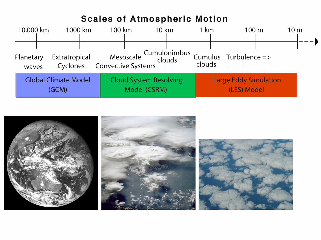
Scales of Atmospheric Motion

1000 km 1 km10 km100 km 10 m100 m10,000 km

Large Eddy Simulation(LES) Model

Global Climate Model(GCM)

Cloud System ResolvingModel (CSRM)

Turbulence =>Cumulusclouds

MesoscaleConvective Systems

ExtratropicalCyclones

Planetary waves

Cumulonimbusclouds

Multiscale Modeling Framework

376 The Atmospheric Boundary Layer

and similarities that can be measured and described.In this chapter we explore the fascinating behaviorof the boundary layer and the turbulent motionswithin it.

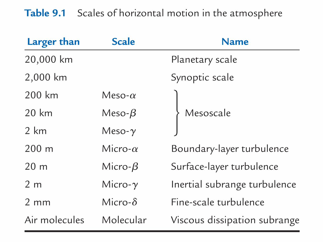
9.1 TurbulenceAtmospheric flow is a complex superposition of manydifferent horizontal scales of motion (Table 9.1),where the “scale” of a phenomenon describes its typi-cal or average size. The largest are planetary-scalecirculations that have sizes comparable to the circum-ference of the Earth. Slightly smaller than planetaryscale are synoptic scale cyclones, anticyclones, andwaves in the jet stream. Medium-size features arecalled mesoscale and include frontal zones, rain bands,the larger thunderstorm and cloud complexes, andvarious terrain-modulated flows.

Smaller yet are the microscales, which containboundary-layer scales of about 2 km, and thesmaller turbulence scales contained within it andwithin clouds. The mesoscale and microscale arefurther subdivided, as indicated in Table 9.1. Thischapter focuses on the microscales, starting with thesmaller ones.

9.1.1 Eddies and Thermals

When flows contain irregular swirls of many sizesthat are superimposed, the flow is said to be turbu-lent. The swirls are often called eddies, but eachindividual eddy is evanescent and quickly disap-pears to be replaced by a succession of differenteddies. When the flow is smooth, it is said to belaminar. Both laminar and turbulent flows can existat different times and locations in the boundarylayer.

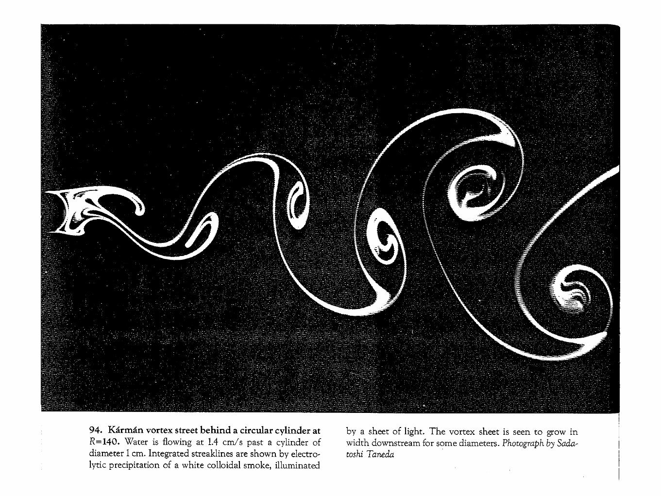
Turbulence can be generated mechanically, ther-mally, and inertially. Mechanical turbulence, alsoknown as forced convection, can form if there isshear in the mean wind. Such shear can be caused byfrictional drag, which causes slower winds near theground than aloft; by wake turbulence, as the windswirls behind obstacles such as trees, buildings, andislands (Fig. 9.2); and by free shear in regions awayfrom any solid surface (Fig. 9.3).

Thermal or convective turbulence, also known asfree convection, consists of plumes or thermals ofwarm air that rises and cold air that sinks due tobuoyancy forces. Near the ground, the rising airis often in the form of intersecting curtains orsheets of updrafts, the intersections of which we canidentify as plumes with diameters about 100 m.Higher in the boundary layer, many such plumesand updraft curtains merge to form larger diameter(!1 km) thermals. For air containing sufficientmoisture, the tops of these thermals contain cumu-lus clouds (Fig. 9.4).

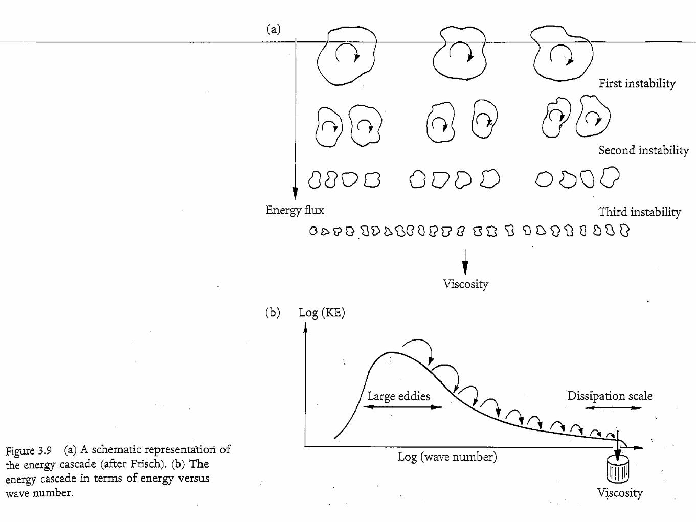
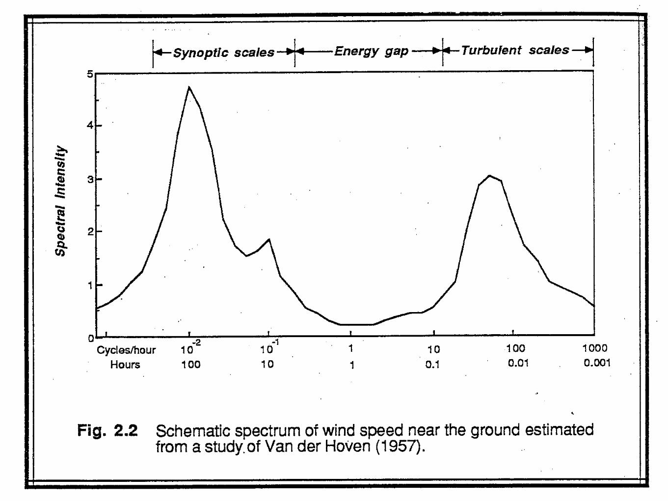
Small eddies can also be generated along theedges of larger eddies, a process called the turbulentcascade, where some of the inertial energy of thelarger eddies is lost to the smaller eddies, as elo-quently described by Richardson’s poem (seeChapter 1). Inertial turbulence is just a special formof shear turbulence, where the shear is generated bylarger eddies. The superposition of all scales of eddymotion can be quantified via an energy spectrum(Fig. 9.5), which indicates how much of the total tur-bulence kinetic energy is associated with each eddyscale.

Table 9.1 Scales of horizontal motion in the atmosphere

Larger than Scale Name

20,000 km Planetary scale

2,000 km Synoptic scale

200 km Meso-!

20 km Meso-" Mesoscale

2 km Meso-#

200 m Micro-! Boundary-layer turbulence

20 m Micro-" Surface-layer turbulence

2 m Micro-# Inertial subrange turbulence

2 mm Micro-$ Fine-scale turbulence

Air molecules Molecular Viscous dissipation subrange

"

Capping Inversion

Boundary Layer

Earth

Free Atmosphere

~11 km

~2 km

Troposphere

ziHei

ght,

z

Horizontal distance, x

Fig. 9.1 Vertical cross section of the Earth and troposphereshowing the atmospheric boundary layer as the lowest portionof the troposphere. [Adapted from Meteorology for Scientists andEngineers, A Technical Companion Book to C. Donald Ahrens’Meteorology Today, 2nd Ed., by Stull, p. 65. Copyright2000. Reprinted with permission of Brooks/Cole, a divisionof Thomson Learning: www.thomsonrights.com. Fax 800-730-22150.]

P732951-Ch09.qxd 9/12/05 7:48 PM Page 376

• Turbulent flow is irregular, quasi-random, and chaotic.

• Laminar flow is smooth and regular.

• Turbulence be generated mechanically, thermally (via buoyancy), and inertially.

Turbulence

• Mechanical turbulence (forced convection) is generated by wind shear.

• Shear can produce flow instabilities.

• Shear occurs

• Near the surface due to frictional drag

• In wakes behind obstacles

• In the jet stream in the free atmosphere

Turbulence

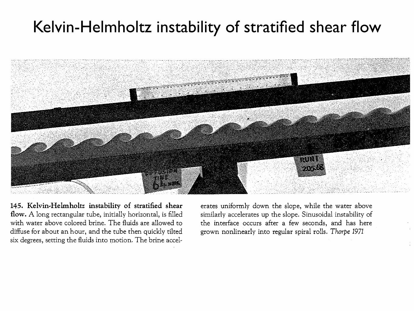
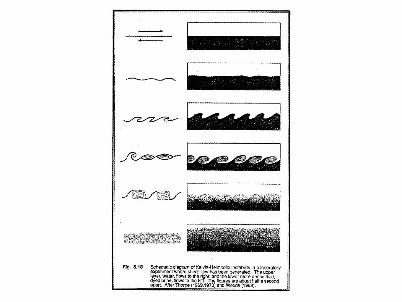
Kelvin-Helmholtz instability of stratified shear flow

2D numerical simulation of Kelvin-Helmholtz instability

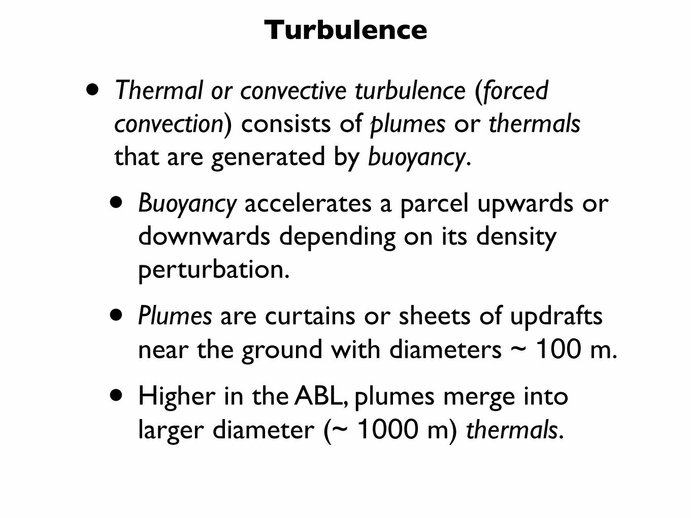
• Thermal or convective turbulence (forced convection) consists of plumes or thermals that are generated by buoyancy.

• Buoyancy accelerates a parcel upwards or downwards depending on its density perturbation.

• Plumes are curtains or sheets of updrafts near the ground with diameters ~ 100 m.

• Higher in the ABL, plumes merge into larger diameter (~ 1000 m) thermals.

Turbulence

9.1 Turbulence 377

Turbulence kinetic energy (TKE) is not conserved.It is continually dissipated into internal energy bymolecular viscosity. This dissipation usually happensat only the smallest size (1 mm diameter) eddies, but

it affects all turbulent scales because of the turbulentcascade of energy from larger to smaller scales. Forturbulence to exist, there must be continual genera-tion of turbulence from shear or buoyancy (usuallyinto the larger scale eddies) to offset the transfer ofkinetic energy down the spectrum of ever-smallereddy sizes toward eventual dissipation. But why doesnature produce turbulence?

(b)

(a)

Fig. 9.2 Karman vortex streets in (a) the laboratory, forwater flowing past a cylinder [From M. Van Dyke, An Album ofFluid Motion, Parabolic Press, Stanford, Calif. (1982) p. 56.],and (b) in the atmosphere, for a cumulus-topped boundarylayer flowing past an island [NASA MODIS imagery].

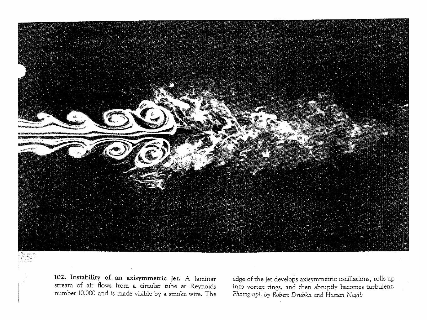
Fig. 9.3 Water tank experiments of a jet of water (white) flow-ing into a tank of clear, still water (black), showing the break-down of laminar flow into turbulence. [Photograph by RobertDrubka and Hassan Nagib. From M. Van Dyke, An Album of FluidMotion, Parabolic Press, Stanford, CA. (1982), p. 60.]

Fig. 9.4 Cumulus clouds fill the tops of (invisible) thermalsof warm rising air. [Photograph courtesy of Art Rangno.]

Tur

bule

nce

Kin

etic

Ene

rgy

per

eddy

siz

e

large eddies(~2 km)

medium eddies(~100 m)

small eddies(~1 cm)

inertial subrange dissipation

productionsubrange

cascade of energy

Fig. 9.5 The spectrum of turbulence kinetic energy. By anal-ogy with Fig. 4.2, the total turbulence kinetic energy (TKE) isgiven by the area under the curve. Production of TKE is at thelarge scales (analogous to the longer wavelengths in the elec-tromagnetic spectrum, as indicated by the colors). TKE cas-cades through medium-size eddies to be dissipated bymolecular viscosity at the small-eddy scale. [Courtesy ofRoland B. Stull.]

P732951-Ch09.qxd 9/12/05 7:48 PM Page 377

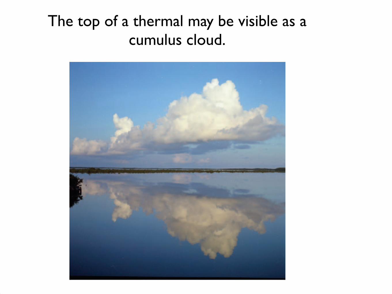
The top of a thermal may be visible as a cumulus cloud.

Cu time-lapse video on class web page

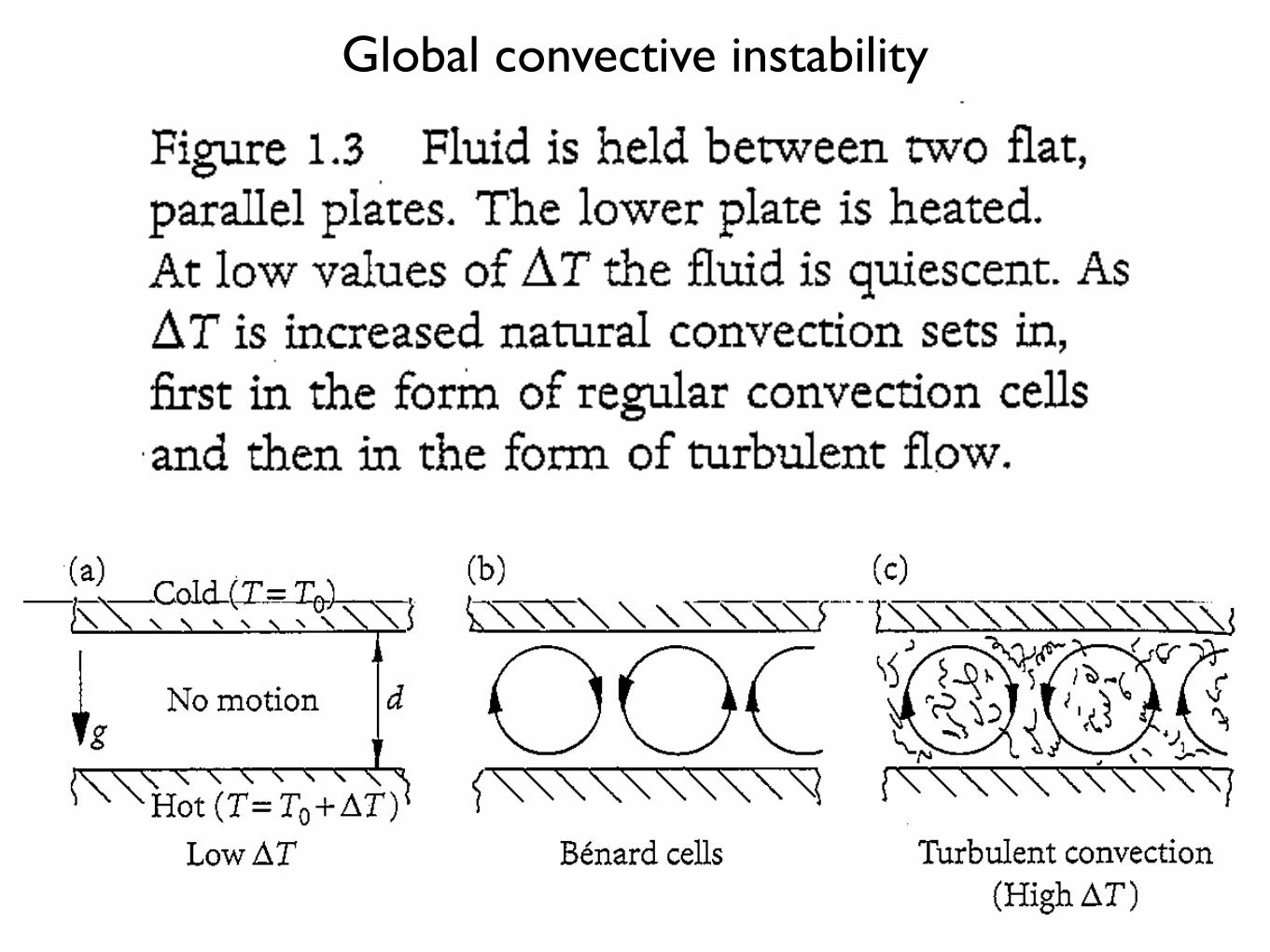
Global convective instability

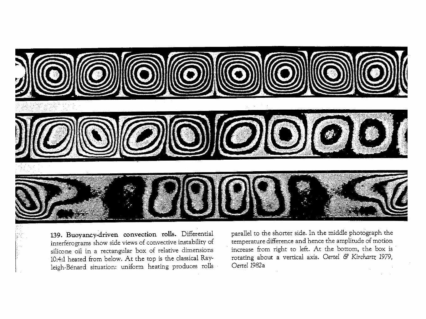
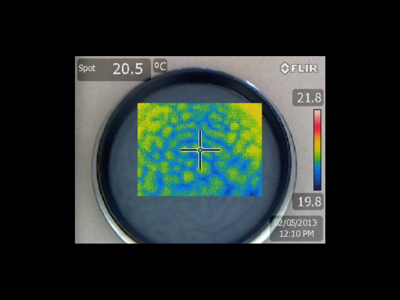
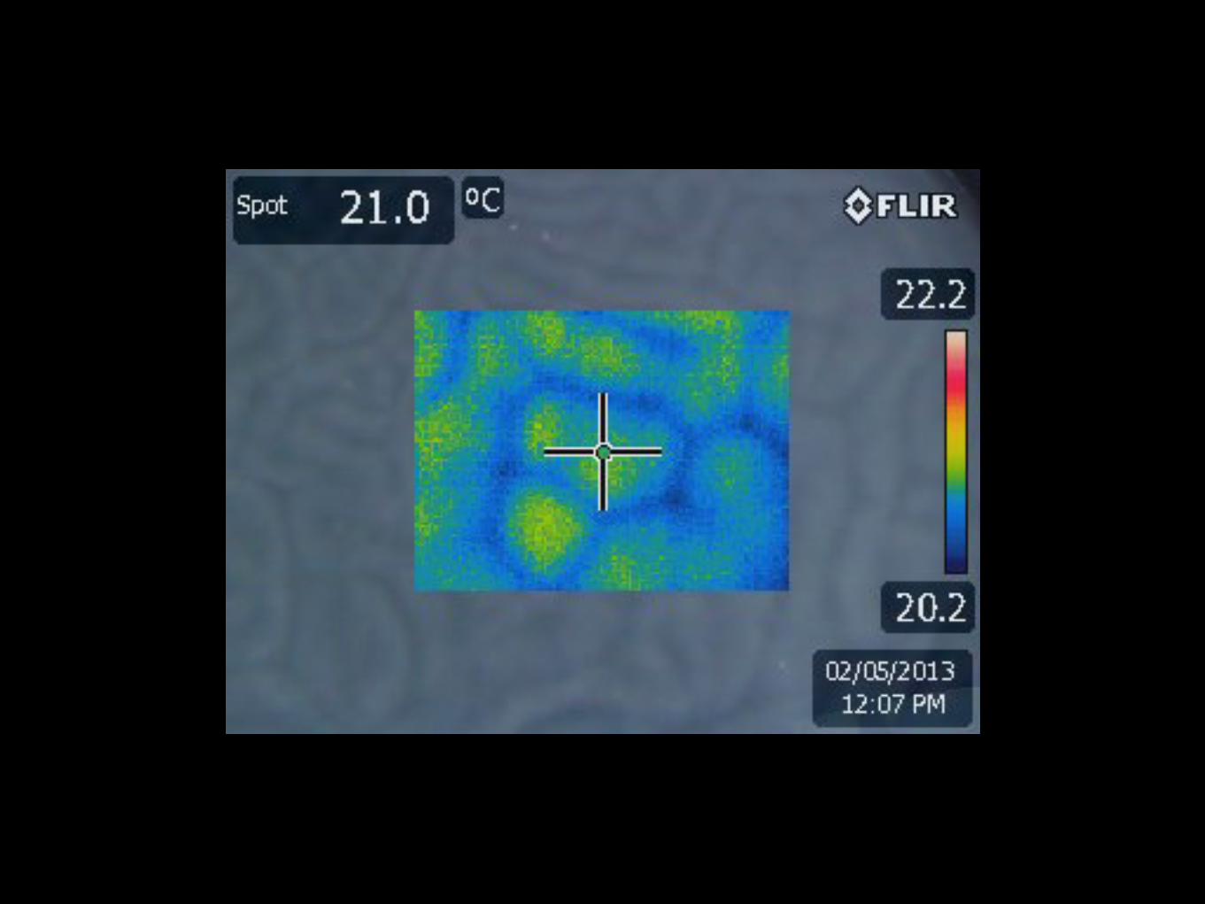
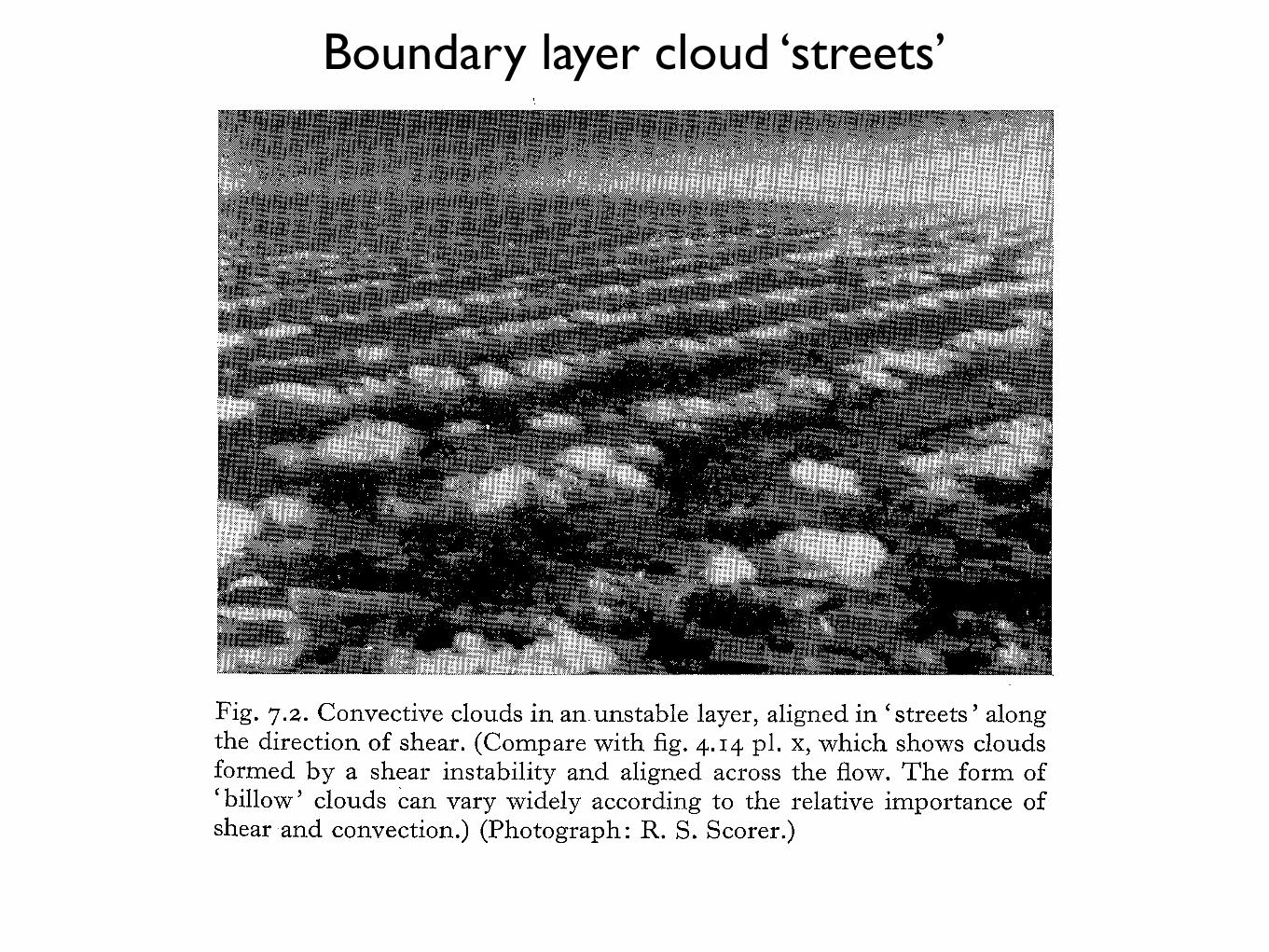
Boundary layer cloud ‘streets’

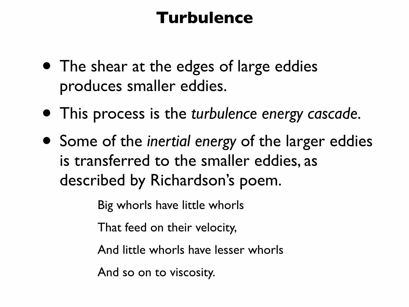
• The shear at the edges of large eddies produces smaller eddies.

• This process is the turbulence energy cascade.

• Some of the inertial energy of the larger eddies is transferred to the smaller eddies, as described by Richardson’s poem.

Big whorls have little whorls

That feed on their velocity,

And little whorls have lesser whorls

And so on to viscosity.

Turbulence

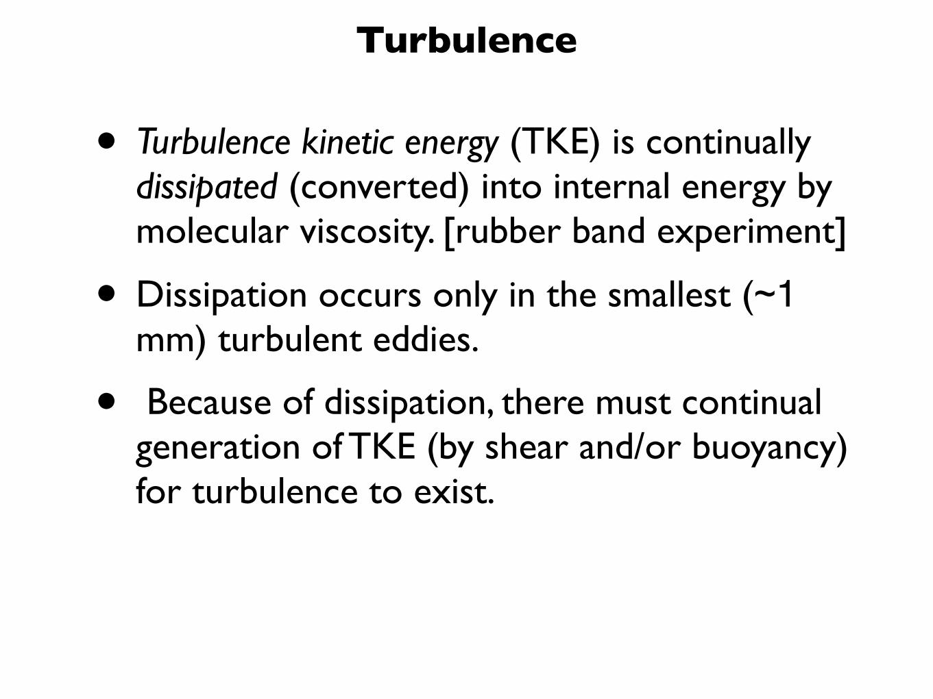
• Turbulence kinetic energy (TKE) is continually dissipated (converted) into internal energy by molecular viscosity. [rubber band experiment]

• Dissipation occurs only in the smallest (~1 mm) turbulent eddies.

• Because of dissipation, there must continual generation of TKE (by shear and/or buoyancy) for turbulence to exist.

Turbulence

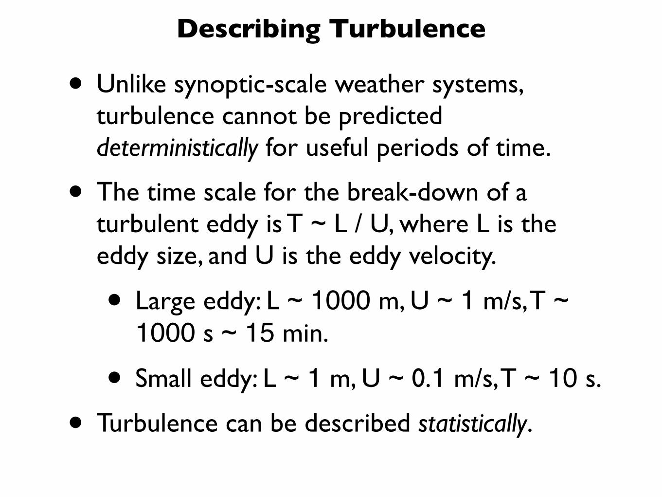
• Unlike synoptic-scale weather systems, turbulence cannot be predicted deterministically for useful periods of time.

• The time scale for the break-down of a turbulent eddy is T ~ L / U, where L is the eddy size, and U is the eddy velocity.

• Large eddy: L ~ 1000 m, U ~ 1 m/s, T ~ 1000 s ~ 15 min.

• Small eddy: L ~ 1 m, U ~ 0.1 m/s, T ~ 10 s.

• Turbulence can be described statistically.

Describing Turbulence

378 The Atmospheric Boundary Layer

Turbulence is a natural response to instabilities inthe flow—a response that tends to reduce the insta-bility. This behavior is analogous to LeChatelier’sprinciple in chemistry. For example, on a sunny daythe warm ground heats the bottom layers of air, mak-ing the air statically unstable. The flow reacts to thisinstability by creating thermal circulations, whichmove warm air up and cold air down until a newequilibrium is reached. Once this convective adjust-ment has occurred, the flow is statically neutral andturbulence ceases. The reason why turbulence canpersist on sunny days is because of continual destabi-lization by external forcings (i.e., heating of theground by the sun), which offsets continual stabiliza-tion by turbulence.

Similar responses are observed for forced turbu-lence. Vertical shear in the horizontal wind is adynamic instability that generates turbulence. Thisturbulence mixes the faster and slower moving air,making the winds more uniform in speed and direc-tion. Once turbulent mixing has reduced the shear,then turbulence ceases. As in the case of convection,persistent mechanical turbulence is possible in theatmosphere only if there is continual destabilizationby external forcings, such as by the larger scaleweather patterns.

Although the human eye and brain can identifyeddies via pattern recognition, the short life span ofindividual eddies renders them difficult to describequantitatively. The equations of thermodynamicsand dynamics described in Chapters 3 and 7 ofthis book can be brought to bear on this problem,but the result is an ability to deterministically simu-late and predict the behavior of each eddy foronly exceptionally short durations. The larger diam-eter thermals can be predicted out to about 15 minto half an hour, but beyond that the predictiveskill approaches zero. For smaller eddies of order100 m, the forecast skill diminishes after only aminute or so. The smallest eddies of order 1 cm to1 mm can be predicted out to only a few seconds.This inability to deterministically forecast turbu-lence out to useful periods of days is a result ofthe highly non-linear nature of turbulent fluiddynamics.

Despite the difficulties of deterministic descrip-tions of turbulence, scientists have been able to cre-ate a statistical description of turbulence. The goalof this approach is to describe the net effect ofmany eddies, rather than the exact behavior of anyindividual eddy.

9.1.2 Statistical Description of Turbulence

When fast-response velocity and temperature sensorsare inserted into turbulent flow, the net effect of thesuperposition of many eddies of all sizes blowing pastthe sensor are temperature and velocity signals thatappear to fluctuate randomly with time (Fig. 9.6).However, close examination of such a trace revealsthat for any half-hour period, there is a well-definedmean temperature and velocity; the range of temper-ature and velocity fluctuations measured is bounded(i.e., no infinite values); and a statistically robust stan-dard deviation of the signal about the mean can becalculated. That is to say, the turbulence is not com-pletely random; it is quasi-random.

Suppose that the velocity components (u, v, w) aresampled at regular time intervals !t and then digitizedand recorded on a computer to form a time series

(9.1)

where i is the index of the data point (corresponding totime t " i!t) for i " 1 to N in a time series of durationT " N ! !t. The u-component of the mean wind ,u

ui " u (i ! !t)

Time (s)

Tem

pera

ture

1°

16 m

0.5 m

2 m

4 m

0 906030

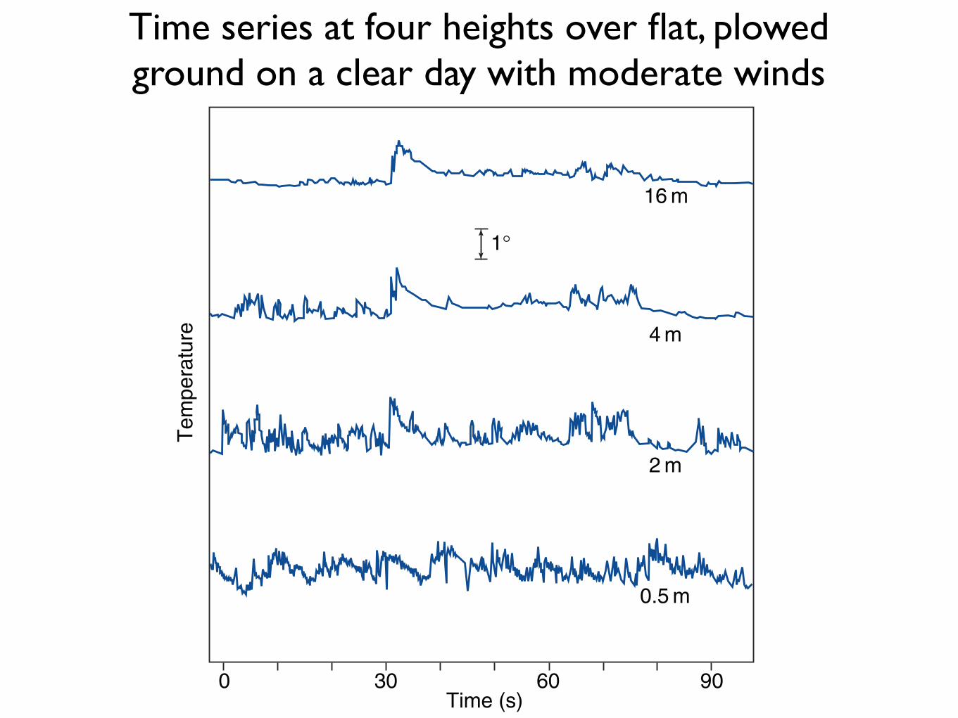
Fig. 9.6 Simultaneous time series of temperature (°C) atfour heights above the ground showing the transition from thesurface layer (bottom 5–10% of the mixed layer) toward themixed layer boundary layer (upper levels of the boundary layer).Observations were taken over flat, plowed ground on a clearday with moderate winds. The top three temperature sensorswere aligned in the vertical; the 0.5 m sensor was located 50 maway from the others. [Courtesy of J. E. Tillman.]

P732951-Ch09.qxd 9/12/05 7:48 PM Page 378

Time series at four heights over flat, plowed ground on a clear day with moderate winds

• Time series of measurements in turbulence show apparently random signals.

• But over a given time period such as 30 minutes, there is a well-defined mean, and a statistically robust standard deviation about the mean.

Statistical Description of Turbulence

Statistical Description of Turbulence

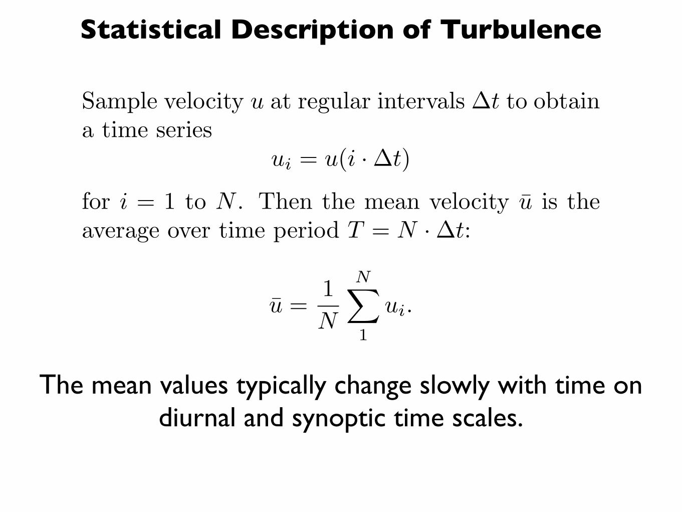
Sample velocity u at regular intervals ∆t to obtaina time series

ui = u(i · ∆t)

for i = 1 to N . Then the mean velocity u is theaverage over time period T = N · ∆t:

u =1N

N�

1

ui.

The mean values typically change slowly with time on diurnal and synoptic time scales.

Statistical Description of Turbulence

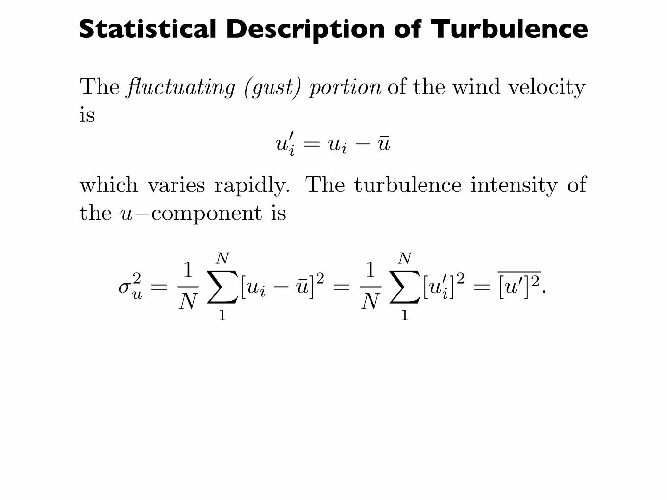
The fluctuating (gust) portion of the wind velocityis

u�i = ui − u

which varies rapidly. The turbulence intensity ofthe u−component is

σ2u =

1N

N�

1

[ui − u]2 =1N

N�

1

[u�i]

2 = [u�]2.

Statistical Description of Turbulence

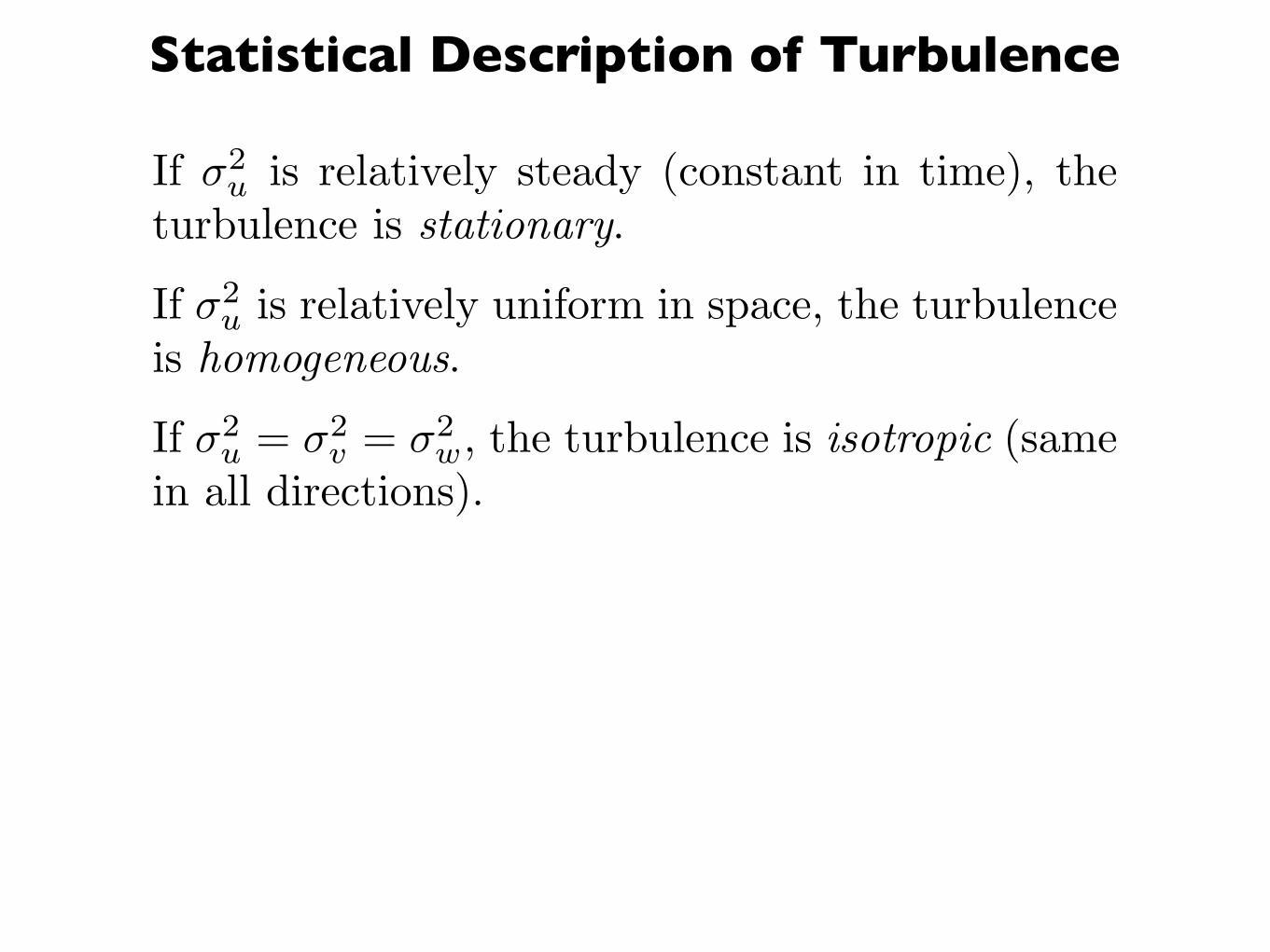
If σ2u is relatively steady (constant in time), the

turbulence is stationary.

If σ2u is relatively uniform in space, the turbulence

is homogeneous.

If σ2u = σ2

v = σ2w, the turbulence is isotropic (same

in all directions).

Statistical Description of Turbulence

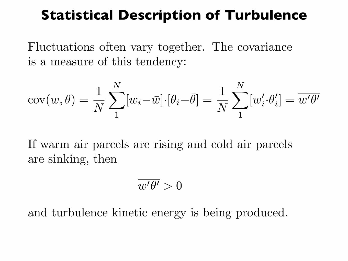
Fluctuations often vary together. The covarianceis a measure of this tendency:

cov(w, θ) =1N

N�

1

[wi−w]·[θi−θ] =1N

N�

1

[w�i·θ�

i] = w�θ�

If warm air parcels are rising and cold air parcelsare sinking, then

w�θ� > 0

and turbulence kinetic energy is being produced.