Embed Size (px)
Citation preview

- 1-
• TURBULENCE IN THE LOWEST ATMOSPHERE
Kyoiti TAKEDA*
CONTENTS
Methods of approach and the scope of the present work. . . . . . . . . . . . . . . . . . 2 The scope of the present work . . . . . . . . . . . . . . . . . . . . . . . . . . . . . . . . . . . . . . . . . . 2 Part I Mean wind velocity . . . . . . . . . . . . . . . . . . . . . . . . . . . . . . . . . . . . . . . . . . . . 3
§ 1. Wind velocity profile .. ............................................ 3 ( I ) Logarithmic law and exponential law .......................... 3
(a) Hellmann's measurement .................................... 3 ( b ) Heywood's measurement. . . . . . . . . . . . . . . . . . . . . . . . . . . . . . . . . . . . . . 3 (c) Prandtl's research ............................................ 3 (d) Best's measurement .......................................... 4 (e) Rossby and Montgomery's theory ............................ 5 ( f ) On the controversy between Sutton and Sverdrup . . . . . . . . . . . . 7 (g) Paeschke's measurements .................................... 8 (h) Takeda's measurements ...................................... 10
( H ) Deviation from logarithmic law ................................ 11 ( i ) Thornthwaite and other's measurements ...................... 11 ( j ) Deacon's measurement ........................................ 11 ( k) Pasquill's measurements ...................................... 14
( Ill ) Summary about the profile and search for the most appropriate formula ........................................................ 15
§ 2. Mixing length and eddy viscosity .................................. 16 § 3. On Thornthwaite's evaporation formula .......................... 19 ~ 4. Summary ........................................................ 21
Part H Irregular or turbulent component of wind ...................... 22 § 1. Introduction ...................................................... 22 § 2. Method of observation ........................................... . 22 § 3. Results of the experiment ........................................ 23
( I ) Mean wind velocity ............................................ 23 ( H ) Energy and intensity of turbulence ............................ 23 ( 1U ) Frequency distribution of the variation of wind velocity ........ 25 ( JV) Frequency distribution of the variation of wind direction ...... 25 ( V ) Coefficient of correlation ...................................... 28 ( \1) Coefficient of horizontal mixing, K" .......................... 29
§ 4. Summary .......................................................... 30 References ................................................................ 31
* Chief, Meteorological Calamity Section, Calamity Prevention Division

- 2 -
Methods of. approach and the scope of the present work
One of the characteristics of the atmospheric turbulence is the participation
of stability of the air layer in the phenomena, and at the same time it makes
the problem more difficult. The effect of stability may be considered by the
three methods as follows:
(1) theoretically
Ross by and Montgomerya:J), and recently Lettau27 l and Kawahara20 l adopted
this method. If the theory is sound, this will give the most reliable results. But
at the present stage the theory »eems to contain some ambiguities or defects. We
shall discuss later some of the equations.
(2) empirically
(a) from the profile of mean wind velocity
Wind velocity is easy to measure and many observations have been
made. If the profile is known we can obtain the stability dependence of eddy
viscosity, mixing length, etc., using widely accepted relations between them.
(b) from the irregdar or turbulent component of wind velocity
Eddy viscosity and mixing length, etc., will be obtained also from the
turbulent component of wind velocity. Ertel's6l formula is well-known, but it
has not been utilized to obtain the stability dependence of the eddy viscosity.
Lettau2'll·24 l,2ol used ''kinetische Austauschformel'' to obtain austausch·coefficient
from his free balloon measurements and got some conclusions about the degree
of turbulence near the cloud. Recently Frankenberger0l succeeded to obtain
a relation between the eddy yiscosity and stability though his results showed
some scattering. This method seems to be interesting but rather difficult, 2nd
only a few measurements have been made.
The scope of the present work
As the theories are not sound at present we will adopt the empirical methods.
In the first part of this paper conceming the profile of mean wind velocity, we
will review studies on wind velocity profile hitherto done by many investigators
(the author inclusive) and give the most reliable one now obtained, because the
primary importance in this method is to get the most exact profile possible,
and then consider the stability dependence of eddy viscosity, mixing length, etc.
In the second part of this paper regarding the turbulent component of wind
velocity the author will describe his own observations, as only a few experiments
in this field have been made. Though his observations do not necessarily give
satisfactory results conceming the stability dependence, yet they seem to be
interesting in some respects.

3
PART I Mean wind velocity
~ 1. Wind velocity profile.
The development of research on wind velocity can be conveniently considered
,dividing into two stages; namely, the former, prewar and war period, in which
the question of whether the profile should be represented by the logarithmic or
the exponential law constitued the main problem; and the latter, postwar period,
in which the existence of deviation from the logarithmic law was recognized
with certainty.
( I ) Logarithmic law and exponential law (a) Hellmann's13l,lJ),u),lol,lfil measurement
One of the most detailed study of wind in the lower atmosphere was due to
Hellmann, who expre[sed results up to the height of 258m. either by logarithmic
formula u=aln(z+c)+b .......................... ( 1)
or by exponential
u=azn .............................. ( 2)
where u denotes the wind velocity at the height z, and a, b, c and n are constants.
He observed that both of them represent the results fairly well, but, above
all, .the exponential profile with
n=5 for z>I6 m.
n=4 for z< 2m.
was best.
(b) Heywood's18 l measurement
The c~ependence of wind velocity on stability
was made clear for the first time by Heywood. Fig. 1 Difference in wind velocitv
From measurements of wind velocity at two · between 95 m. and 13m. in relation heights z=95 m. and z= 13m. with simultaneous to difference in temperature bet
temperature measurements, he observed that at
constant uo,, Uo5-U13 increased from negative to
positive values of r~,--Tl3, and at constant To,
T13, uo5-uu increased with uJ, where T denotes
temperature. Fig. 1 and 2 show his results. In
fig. 2 he draws curves after Taylor's5~l theoreti
cal conclusion. But Taylor's theory was based
upon assmnptions of finite surface wind and
constant eddy viscosity, both of which are
recognized to be not the case in the lowest
layers of the atmosphere.
(c) Prandtl's31 l research
Prandtl applied results of aerodynamics to
ween 87 m. and 13 m.
Oi::+2DF ... )( +:•F .. :.. 0 ······0 -r~r·· o -2"F .. o
Fig. 2. Difference in wind velocity between 95 m. and 13m. in relation to wind velocity at 95 m. for fixed values of temperature gradient.

the lowest atmosphere. The definition of shearing stress , 1s
au <=A-,-, ............................ (3) oz
where A is austam:ch-coefficient. He improved this expre:csion and deduced
'= pl2( ~i y, .......................... ( 4)
in which only the geometric quantity l (mixing length) is contained except air
density p. The results of aerodynamics showed that in the absence of
stability l was proportional to z and the proportionality factor was equal to
0.4, so (4) becomes
-~: = 2~5 J-; . . ......................... ( 5)
If ' is assumed to be constant with z in the lowest atmosphere, e. g. lowest
50 or 100m., (5) is easily integrated and gives
u = 2.5 I 'E_[ n z, .......................... ( 6 ) V p z,J
where zo is an integration constant which adjust itself that at the surface of the
roughness u equals to the actual velocity. zo is considered to be in a definite
relation to the height of the roughness lz and in the aerodynamics it was found
that
k Zo= 30 , ............................ ( 7)
where k means the diameter of a grain of sand adhered to the wall. Instead
of 30, smaller values are found in the atmosphere after that, e. g. 7.35 (Paeschke23 l).
and 3 (Shiotani and YamamotooGl, and Takeda15l).
Prandtl further made some discussions about the non-adiabatic atmosphere,
but without a remarkable conclusion.
The significance of the Prandtl's analysis seems to lie in the fact that in
the adiabatic atmosphere the wind profile is shown to be represented by the
logarithmic law, and since then the exponential law has been used only in cases
where theoretical treatments become especially simple.
(d) Best's1l measurement
One of the most detailed measurements of wind and temperature in the
lowest atmosphere was done by Best. The stability depependence U(z) (wind
velocity at height z expressed as percentages of the simultaneous velocity at
1m.) was given by him as follows:
Table 1.
I 2.5em.l 5 em. \10 em. I, 25 em. I 50 em.l100em.\200em.l 506em.
-3o FJm. I
42.9 I 52.0 1· 66.7 I 81.0! 90.3 100 I
107. 1 I Temperature f Zero 36.4 49.0 63.0 . 79.2 90.3 100 111.7 122.5 Gradient
l -1- 1" F.im. I
I I 33.9 47.5 60.0 77.1 89.5 100 114.3

-5-
He observed that in the adiabatic atmosphere U(z) is in the linear relation
with log(z-1). In the non-adiabatic atmosphere he could not work with logarith
mic law, but adopting exponential law (2) he obtained stability dependence of
n as is shown in table 2 for the height interval from 25 em. to 2m.
Table 2. Variation of index in exponential law with temperature gradient
Temperature Gradient Index Simultaneous Conditions -------~~ ~-~-----------------------------
-3.0°F.;"m.
Zero
+ 1.0°F./m.
7. 15
5.87
5.27
Layer 25 em. to 2 m.
Velocity at 1 m. between 1. 5 m./sec.
and 4.0 m./sec.
From the table it is seen that the index n decreases as the air layer becomes
stable.
(e) Rossby and Montgomery's3 ~l theory
The first theoretical treatment of the stability dependence of turbulence in
the lowest atmosphere was attempted by Rossby and Montgomery. They started
from two assumptions :
( I ) an energy equation
P( ~~ ): = t~( ~~ y + 11: ~~ l~, ................ C 8 ) where (} represents the potential temperature and g the acceleration of gravity
and suffix s is applied to denote quantities in the stratified atmosphere, and 11
is a proportionality factor (40 according to Rossby and Montgomery) which has
been called Rossby's constant subsequently,
( n ) constancy of shearing stress with stability
\/"r =t,(aau~) =l aau, ...................... (9) p z ·' z
and deduced
where
V.x.=frictional velocity=J', .................. (11) p
and
r~= 11g ~(} . .......................... (12) (j oz
Integration of (10) gives
U = V~,:- r{ z+z,l_f-2( -1)-l p(p+l) \ (1"') k 1.. n z~ P n 2 J ' · · · · · · · · · · · · '"'
where
p=(-a!!__) J(au) = /1+1 /I 4r"(z+z0 ) 2
az , 1 az ad v 2 2 \ + (vkJ
= Uad+ vk. { 2 (p-1) -ln p(p; 1) } , .................... (14)

-6-
and
u,d= V.x. ln_z;_+zn ........................ (15) k Zo
denotes the value of u in the adiabatic atmosphere. Further they gave the eddy
viscosity coefficient as
and the expression
u-u~~rt
represented graphicaly.
..... 0. 0. 0 0 ...... 0. 0 •• (16)
=f(p) =2 (p-1)-ln p(p+l) 2
0 0 0 0 •••• 00 00 •• (17)
The wind velocity formula (13) is complicated and has a form which makes
the treatment not easy, but it is shown at once that for larger values of stability
one has, with increasing degree of accuracy v--
u--r Lv-.z-. .......................... os) J vk.
With the formula thus obtained, they tried to explain Heywood's data and
showed a good agreement between the theory and experiment as is seen in fig.
3. Moreover they showed a greater part of Hellmann's experimental points lie
between the two theoretical limits,i. e.
Fig. 3. Diurnal variation of the vertical wind distribution (u32-
urGl I (u!6-u2) for different wind velocities and seasons.
i. e.
and obtained
in the adiabatic atmosphere
U.J3-U!6 =[n 32/16 =O 33 uw-u2 ln 16!2 ·
in the most stable atmosphere
u.J2-ura v'32-v'I6 uru-u2 - v'J.s-v' 2 °'64
as is seen in fig. 3.
Rossby and Montgomery did not take into
account the variation of lapse rate of tempera
ture with height which is the common pheno
menon in the lowest atmosphere. Later
Sverdntpm put
1
{} = Oo+b(z+zo);;. .......................... (19)

- 7
u=u,,+ n ~kv.~. [ 2(p'-1)-ln p'(p;+l) \J .......... (21) n+1
and
K=- -~_k(z+zo)v.,.. . ............... (22) j 1 ..L 1 j , n+l \ -i . -2-y ] + 4 rr(z+zo~-2-
(~}
where u," is the same as in (15), and p' is obtained by substituting (20) in (14).
From experiment over the snow field Sverdrup found
a=11.
Rossby and Montgomery's theory seemed to receive general recognition at
the time, but after that its validity came into question. For instance, as to the
fundamental assumption ( H ) Brunt wrote in his PHYSICAL AND DYNAMICAL
METEOROLOGY that it was "doubtful asmmption," and really this is contrary
to our experience that in the stable atmosphere layers of air become easy to
glide over each other and make shearing stress smaller. As to the fundamental
assumption ( I ) the author48l recently described as "groundless," because a correct
-energy equation must be the equation of energy dissipation which is deduced
from the equation of motion. So it is natural that a should vary with stability
as recently found out by Deacon"l, i. e. for extremely unstable condition a=e2
and for markedly stable condition a=e20.
Moreover, Rossby and Montgomery and also Sverdrup considered that the
wind profile was the ,;arne in the adiabatic and unstable atmosphere which was
supported by Sverdrup's experiment of a few observational heights, but it is now
widely accepted that it is not the case. (In the later paper Sverdrup"'> seems to
consider that the profile is different in the adiabatic and unstable atmosphere.)
(f) On the controversy between Sutton and Sverdrup
In 1936 Sutton33 l remarked that if the wind profile was represented by
_!!_=tn(.!!Z._+ l );!ln(a+l) .................... (23) llt Zt
where Ut is the wdue of u at the height Zt, the parameter a provided a very
sensitive indicator of turbulence--i. e. a increased very rapidly on the lapse
side. A<?;ainst him Sverdrupm, based upon Rossby and Montgomery's theory,
wrote that (23) was valid only in the adiabatic atmosphere and enormous range
of the values of a which Sutton obtained from temperature and wind observa
tions at two levels showed not that a was a sensitive indicator of turbulence,
but that the logarithmic law failed to hold good when the temperature gradient
differed from the adiabatic.
In the subsequent paper Suttonm criticized Sverdrup's theory and wrote
"like all modern mathematical studies on atmospheric turbulence, this analisis is
not exact, and depends in the first instance on certain assumptions. An appeal
to experiment is therefore essential". He then showed that Best's observation

-8-
was represented more cosely by logarithmic than power law, and interpreted z0
( =:1 ), as defined by Prandtl, to be possible of being a function of stability.
But Sverdrup44) still maintained the validity of tne theory, and, contrary to
Sutton's opinion, tried to show that the Best's data c~ n be interpreted differently
and lend strong support to the statements that the roughness length was a
characteristic physical constant and that the influence of stability can be
expressed by means of another constant r1.
Since the nthis subject seems to have been discussed by none else but Takeda45 )
who, recognizing the defect of the theory and observing that his own wind
profile experiment could be represented by logarithmic law, supported Sutton.
(Recently Halstead11 ) describes that "since there were. no observations of
sufficient accuracy to provide sound judgment, controversies such as that between
Sverdrup and Sutton were never clearly resolved.") And about fifteen years have
elapsed since Sutton first published his paper, and meanwhile precise experimental
data have increased, and Sutton40 ) himself describes recently that if the greater
height than 2 or 3 m. above the ground is considered, the evidence that shows
the failure of logarithmic law is being accumulated.
As to the theory also some developments have been made. So Kawahara"0 )
tried to apply Karman's19 ) energy equations to the lowest atmosphere and Lettaum
attempted to improve the Rossby and Montgomery's theory. But as Kawahara
uses some assumptions, such as the constancy of turbulent energy (u'"+v' 2 +w'")
with height, which need more verifications in the atmosphere, and as Lettau's
treatment contains some ambiguities, both theories seem still not to be sound.
Lettau tries to improve the Ross by and Montgomery's energy equation ( I )
by replacing it with an acceleration equation, which seems to be incapable of
being deduced from the equation of motion just as the energy equation is
incapable of being deduced from the equation of energy dissipation. But the
author considers if the Lettau's acceleration equation is true it should be that
which can be deduced from the equation of motion.
Recently Halsteadll) considers that r is not constant with height in the surface
layer and putting r = ro+bz (where ro is the value of r at the surface and b~O·
stable for adiabatic atmosphere) gets some conclusions which can explain actual
unstable I
results. But to consider r variable in the surface layer produces other difficulty,
for instance, Halstead's assumption makes ~: >O for stable atmosphere, i. e.
the air IS accelerated at night (and vice versa in the daytime) which is
contrary to the case.
(g) Paeschke's38) measurements
A set of measurements on wind-, temperature-, and humidity profile was
made by Paeschke, who found that the exponent n varied from 3.0 to 5.0;

-9-
became smaller as the roughness of the surface decreased, and, on the other
hand, represented wind profile by a logarithmic law
u = ~k":c-ln z-d , .......................... (24) Zo
where d is a height introduced to adjust to various roughr:.ess, and Zn has the
same meaning as before. Paeschke put
k Zo=7:35• .............................. (25)
where k is the height of unevenness of the surface or the height of the overgrowth.
From direct measurements of stalk-length d, and u and z he showed that k = d
though there was a fair scattering of values.
Paeschke made some analysis concerning with stability but not with logari
thmic profile, so it is of little interest to the author.
It may be added here concerning the form of ln(z±d). There still remain
some uncertainties as to the form of the logarithmic formula in the adiabatic
case. For Rossby ancl MontgomerY:1 ~l, Sverdrup42 l and Sutton38 l adopted the type
u=aln z+zo, .......................... (26) Zu
while Paeschke23 l and Thornthwaite and Holzman-'") used
u=aln z·-d Zo
...................... (27)
So we are at a loss which to select.
If there is a surface, whose roughness shall be chan:.cterized by a quantity
h, and if the wind profile over the surface is represented by
u=a[n3.._, ............................ (28) Zo
we can assume h is proportional to zu, i. e.
h=rzo. . ............................. (29)
If the form and height are constant and only the density of the roughness varies,
we will probably obtain profile that shows reference surface elevated or lowered
Ul
~ zl z
~ I
i 1 ! ..c:,
~ L ... L_ ___ _.___ u u Fig. 4. Wind profile and density of element.
A: Density of B: Density of C: Density of roughness: medium roughness: large roughness: small
u~zn_z_ u~lnz=d u~lnz+d ~ ~ z
as is shown in fig. 4. If the form of the curve remains the same, we obtain
for B and C of the figure
-10-
u=aln z'fd ........................... (:10) Zn
But it is doubtful whether the curve remains the same after the density varies.
We may also obtain in that case
If we assume
u=aln-2 -(o '
where (u=Zo'fd. . ............... (31)
h=r'(n, .............................. (32)
r' is, of course, different from r. The expE:rience of the author shows that over
various natural surfaces u is proportional to l nz in the adiabatic case, hence
that the formula (31) holds, and it is not necessary to use (26) or (27). So in
view of the pure empirical nature of the formula the author considers it sufficient
to adopt (28) and only when experiments (made near the roughness height)
show some deviation from (28) we should use (30) in agreement with conclusion
obtained by Deacon4 l that in conditions of neutral stability the logarithmic law
·Can represent the profile between heights of 1m. and 13m. over the grass of
various heights with great accuracy, provided that both Zn ancl. d are chm:en
independently to give the best fit.
(h) Takeda's45l measurements
Nineteen measurements of wind- and temperature profile either in stable or
unstable conditions were made by the author over a natural surface with not
small and not uniform roughness (maximum height of the shrub reached
about 1.5 m.). Obtained results at 4 heights up to 5 m. showed that the exponent
n varied with height and stability from 0.5 to 4.0 (increasing with height and
decreasing with stability), and that the logarithmic law was better fitted than
the exponential law, and if zo was considered to vary according to stability, i. e.
increasing with stability, the simple logarithmic formula
u=a[n_3____ ............................ (33) Zo
fitted well in the limit of the experimental error. From the fact that the
logarithmic law held also in the non-adiabatic atmosphere the author deduced
for the stability dependence of K, v.,__,, and k as follows :
K= IS 1+aR;
. . . . . . . . . . . . . . . . . . . . . . . . . . (34)
V.x.s = / V.;c , ........................ (35) v l+aR;
and
k k,,-v l+aK ' ...... · · .. · · · · ........ · · .. (3G)
where R; (Richardson's no.)=::: j ( ~~ Y, and suffix s is applied to denote
.quantities in the stratified atmosphere. But the deviation from the logarithmic
11-
law obtained recently makes the author adopt another formulae which will be
described latt:r.
( IT ) Deviation from logarithmic law
(i) Thornthwaite and other's measurements
Though :come deviations from log<.rith.mic law were observed in Best's and
Sverdrup'~" data they were not so powerful as to d:.im their existence, for in
those days the problem of the profile being represented by logarithm or exponen
tial itself was not settled and Sverdrup's"') data were obtained over snowfield
with only 3 heights of measurement. But in the wm·tiiT..e the existence of the
deviation was being observed more certa:nly. So Thornthw<.ite and Halstead51 )
from measurements of profile by 6 heights up to 20ft. found the deviation 2nd
proposed a rather untraceable combination of logarithmic and power terms 1
u = (}!_z_z = l nzo -)·~' lna ' •• 0 •••• 0 ••••••••• 0 •••••• (37)
where the exponent p was expected "to vary between 2.0 with fully developed
turbulence and some value less than 1.0 when turbulence reaches its smallest
actual value." To quote Sheppard dter Halstead11): "In this respect the most
notable published profiles are those of Thornthwaite and Kaser (1943), taken
0ver a flat field in Ohio at up to 12 levels between 0.5 ft. and. 28ft. The u,
l nz curves for successive hours throughout the day show a marked progression
of form, being concave to the u-axis between sunset and sunrise, that is during
the period of temperature inversion, linear shortly after sunrise anc. before sunset
when conditions are approximately dry-adiabatic and convex to the u·cxis during
the central daylight hours of superadiabatic lapse rate. Halstead (1943) has
shown that the curvature of their
profiles is intimately related with
the temperature difference which
was recorded between 2ft. and 8ft."
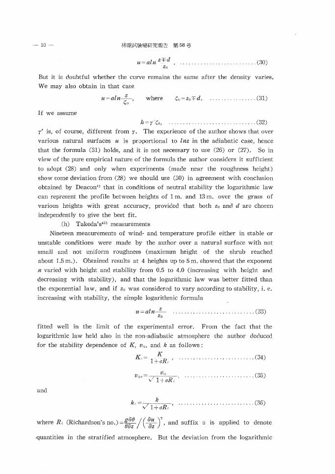
(j) Deacon'sn measurement
One of the most systematic
relations between the deviation and
stability is given by Deacon recently, z~-_,...----;~'--....,.;::...;.........;~+-~.?.....!-i-..:....-1
who arranged his data according to
the mean Richardson's no. between
the height 4 and 0.5 m., ]":o-o- It is
reproduced on fig. 5. It is clear
· from the figure that m unstable
conditions u, log z distribution is
convex to the u-axis and in stable
conditions it has an opposite curva
ture, and the curvature itself is large
Fig. 5. Variation of wind distribution with. stability.

-12-
as the difference from acliabaticity becomes large.
He found that the formula of the type
~~ =az-8 , ............................ (38)
where for unstable condition,
{3 = 1 for neutral condition,
!3<1 for stable condition,
represents the data quite closely, and gave the variation of {3 with stability in a
figure.
The integration of (38) leads to a new profile
az6-·8 ( ( z )t-~ "\ u=-1--{3 l z~ -] J' ...................... (39)
and if
a= v.,. (40) kz6-~ ' · · · · · · · · · · · · · · · · · · · · · · · · · · · ·
(39) becomes
_ V.x. U- k(1-{3) [ ( z )!·-~ } z;;- -1 ..................... (41)
Deacon states that, strictly speaking, the parameter {3 is not constant with
height and the deviation of {3 from 1 increases to mme extent with height. But
the non-constancy of {3 with height seems to arise from the fact that Deacon
makes zo constant with stability. Deacon, ignoring actual variation, considers
zo is constant, because as the Richardson's no. varies almost linearly with height
the effect of buoyancy must become very small in the layer near the earth's
surface and results based on many observations show that the effect of tempera-
ture gradient upon velocity distribution decreases as the surface is approached
as foiiows:
Ratio of wind
8:4 4:2
2: 1
m.
m.
m.
1: 0.5m.
Percentage variationt of wind on the given stability range
7.2 5.5
4.2 2.6
t stability range from -0.1 to +0.06
But though the Richardson no. varies almost linearly with height, it seems
dangerous to extrapolate this to the layer just above the roughness, and,
moreover, it may be shown
_dd (( u"= )., -( u2=) J>o, .................... (42) z \ u= " u= 1
where suffix 1 shows the unstable case and 2 the stable one, is valid in the
height interval of z observed by Deacon (4m.-0.5m.) even though z0 varies.
For adopting Deacon's formula (39) we have

(2z) 1-f3-z6-f3
zl-f3_ztf3
-- 13-
...................... (43)
If {3 and zu is considered to vary with stability and ( 43) is substituted in
the left-hand side of (42) we have
(1-{3)z-!3zl-f3 (1-21-ll) (1-{3)z-llzl-f3 (1-21-!3)
:zce~J2 -( z::,' )J=( (zl-{3:__z6-f3)2 )2 --( (z1-(3~za f3) 2 )1. (44)
From Deacon's results we have
case 1:
case 2:
]_1 : 0 .c,= -0.1,
J,: ll·5= +0.06,
f3t=1.10,
f3e =0.92,
Zo1 =0.4!1 em.,
Zo2=0.lO em.
If these values are substituted m ( 44) we can obtain the domain of z satisfying ( 42), and get
z>0.88 em. . ............................. (45)
The lowest height adopted by Deacon was 50 em., and hence Deacon's
suggestion, that the effect of stability on wind velocity becomes smaller as the
earth's surface is approached, will not prove the constancy of zo.
The form of a will be examined next. Deacon expands the right-hand side
of the equation (39) and comparing it with the equation which rs valid in the
adiabatic condition he obtains (40). But it is easily seen that a may have a
form
a= 7i§i~13 , ............................ (46)
where ( c.enotes an arbitrary length in place of zo. This is absurd, so we should
not expand (39) and put {3 =] carelessly. A correct form of a will be obtained
from (39) and
........................ (47)
where U cl.enotes the velocity at z=zt, as follows:
a=__Q~l-~)__ ........................... (48) zt- -za-(3
In the case of the adiabatic condition, {3 = 1, and U = v., fn_z_ so a beco-k Z1 '
mes
a = v.,., (49) k ............................... .
But we should not expect that this relation holds also in the nonadiabatic
atmosphere. Deacon then obtains a formula of eddy viscosiy as follows:
K = kv.;:.zo( ~ J, ........................ (!:10)
which should be corrected to

--·· 14 -
v2 (zl-~ -zl-~) K= * ~(1-/3°) z!l . ...................... (51)
(k) Pasquill's20 l measurements
The most interesting simultaneous measurements of wind velocity, temperature
and humidity are made by Pasquill at 6 heights up to 2 m. It is extremely
remarkable that wind velocity, temperature and humidity show the :::-arne deviation
from the logarithmic profile as is seen from fig. 6. From the figure it seems
Fig. 6. Vertical profiles of absolute humidity, wind speed and air temperature above short grass.
probable that wind, temperature ancl. humidity distribution in the lowest
layer are dtermined by the same
agency--turbulence. But the tem-perature distribution is shown by
the author to have a greater devia
tion than the other two. This may
be due to the effect of buoyancy or
radiation, but we shall need more experiment to determine this effect.
It may be adc.ed that Pasquill, trying to verify the equdity of K and. K,.
(coefficient of eddy diffusivity for water vapour) experimentally, used
= k3( ~ y~-2 (which is easily deduced from ( 41) and (50)) and asst.:.ming that z,J
is constant with stability calculated this value from his wind observations and
compared it with experimentally obtained K,/ Z 3 a;; . He could conclude that
K = K,. in the unstable as well as in the adiabatic cases, but could not conclude
that K = K,. in the stable case as the values of K j z3 {Z:- became too smalL
If, on the contrary, (39) and the corrected formulae (48) and (51) are used, we
can obtain au v~ Cztil- z6-!3) ,~,3-'~
K/z---az u~(I-/3) 3 z ................... (52)
Assuming the value of V.x./U = l/14.4, which is obtained in the adiabatic cmoe,
is constant also for the non-adiabatic case, we can evaluate K j z2 ~~ as shown
in the table. It is seen that the values are in good agTeement for all cases,
though they are somewhat smaller especially in the unstable case. But it seems
to the author that the experimental verification of the equality of K and K,. is
given for all conditions of stability of the atmosphere.
Table
Richardson's number -0. 125 -0. J0 ; -0.05 I 0 +0.05 I +0. 10 ' +O. 125 I .
K jz2.!!!_ 0.42 0.37
I
0.26 - 0.06 0.016 0.005 Pasquill's value ( / "~~
K,. Z"-- 0.39 0.34 0.24 - 0.11 0.07 0.06 I iJz
I Takeda's value !(/" iJu 0.25 0.24 0.22 0.16 0.10 0.06 0.04 - z·-a-z

- 15 --
( Ill ) Summary about the profile and search for the most appropriate
formula.
Now we have come to the stage of summarizing profiles and searching for
the most appropriate formula.
(a) If the exponential law
u==azu ..... , ........................ (53)
is to be applied:
n varies with z, inceasing as z becomes large ......................... .
. . . . . . . . . . . . . . . . . . . . . . . . . . . . Hellmann1"J,JeJ,HJ,l.>J,lul, Eestll, Takeda4"l,
n varies with roughness, increasing as roughness height becomes :::mall
. . . . . . . . . . . . . . . . . . . . . . . . . . . . . . . . . . . . . . . . . . . . . . . . . . . . . . . . . . Paeschke"3l,
n varies with stability, increasing as the layer becomes less stable ..... .
. . . . . . . . . . . ·. . . . . . . . . . . . . . . . . . . . . . . . . . . . . . . . . . . . . . . . . Best 1l, Takeda 451 •
Values of n are found to vary from O.!J to 5 in the atmosphere.
(b) If the logarithmic law
u=alnz+b .............................. (54)
is to be applied :
Many observations are represented by this law well and, above all, almost
exactly for the adiabatic case.
When the roughness of the surface has some particular feature instead of
(54) for the adiabatic case
u=aln(z+zo)+b .... Rossby and Montgomery3~l, Sverdrup4~l, Sutton"8l, .. (55)
or
u = aln(z-d) +b ........ Bestll, Paeschke38l, .. (56)
will be better fitted.
If (54) is written as
u=aln-z_, ............................ (57) Zu
Zo varies with stability, increasing as the air layer becomes
stable ............ Thornthwaite and Holzman"31 , Suttonm, Takeda'1'l.
(c) For the more precise measurements, deviation from logarithmic law
has been observed. Some formulae are proposed in order to give the best fit,
i. e.
theoretically :
u =at n(z + z.J), F(z) .. Ross by and Montgomery3~l, Sverdrup4"l, Lettau37l, .. (58)
u= alnz+bz+c ............ Kawahara"0l, HalsteacJ11l, .. (59)
empirically :
( ,1
u = aln ~ )1> ........ Thomthwaite and Halstead'll, .. (60)
( ( z )1 -~ } u=a\_ - -1 Zu.
...................... Deacon41 , .. (61)

- 16-
u=alnz+bln2z+c ........................ Takeda-17l.(G2)
The author has shown that the formula of the type (61) or (62) is better
fitted to Best's and Pa:cquill's data than that of the type (59).
It should be mentioned here about the variability of Zo with stability. As
described above Zo is an integration constant which adjw:;ts itself that at the
surface of the roughness u equals to the actual velocity. If zo is regarded as
an unknown parameter and obtained from actual profile, it will be found that
it does vary with stability. But there is a group of researchers who consider
that Zo is a physically definable height and is not influenced by stability.
To this group belong Ro:csby and Montgomery:l2l, Sverdrup·13l, Kawahara~"> and
Deacon·'l. On the other hand Suttonm, Thornthwaite and Holzman53 l, and
Takeda·1"l, consider that Zo may vary with stability, i. e. increasing as the air
layer becomes stable (in a recent paper the author 1GJ has shown that z0 d.ecreases
with stability so long as the formula representing the deviation from the logarith
mic law, such as Deacon's generalized exponential formula or Takeda's gene
ralized logarithmic formula, is adopted).
In this connection it should be stated that the result obtained by Lettaum
is very remarkable. For Lettau distingishes the physically definable rouglmess
height Zo, which does not vary with stability, from the integTation constant
"zo", which is hitherto considered to vary in actual cases, and d.ec1.uced a relation
"zu''"e·z( -~i }'', .......................... (G3)
where X and Y denote some functions of stability. This relation (63) implies
that "zo" is a function of z, so we shall obtain different values of "z0 " if
different reference height is used. But there seems to exist no experiment now
that can ascertain this expression.
After all, though the theoretical ground may be wanting, Deacon's formula
with variable Zo, i. e. decreasing with stability, seems to the author to be the
most simple and the best fitted to experiments at present, and it will be adopted
as the starting point of the following analysis.
or
for
§ 2. Mixing length and eddy viscocity
Having decided to adopt Deacon's formula azl-/3
_ o r ( z )l--{3 _ 1. ~ U- l-!3 \. Zo 1 J, ...................... (o4)
au a-z=az-!3, ............................ (65)
13>1 unstable case,
j3 = 1 adiabatic case,
13<1 stable case,

-17-
where z11. a and {3 are parameters depending only on the stability, as our starting
point, we now proceed to determine the mixing length and the eddy viscosity in
relation to stability. The widely accepted formulaem between the mixing
length, the eddy viscocity and the frictional velocity are
ot£ _ ~ K-8i - v.x-, ............................ (66)
and
l_§J~ =v, .. ............................ (67)
If we assume that these formulae hold also in the non-adiabatic atmosphere
and comparing (65) and (67) we can obtain
~"- = arfJ. . ........................... (68)
v.,-:. shall be assumed here to be independent of z with English researchers"l' 41 l
though it may depend on stability. We have, then,
l ~zfl, ................................ (69)
or
l=A({3)zfJ, ............................ (70)
where A is a proporlionality factor depending only on stability. As [3 is shown
to be determined only by the Richardson's number at a certain height, it is
convenient to adopt lias an index representing stability of the atmosphere because
it does not contain z. But in the adiabatic atmosphere (70) must be reduced to
l = kz, where k = 0.4, ...................... (71)
so we can put instead of (70)
l = kh(ii)zfl. . ........................... (72)
With· this h(/3) the velocity distribution becomes from (64) 2nd (68)
u= __ v.,. --(z1-fl-zl-fJ) k(l--{3)h 0 ,
( - v.,. ) (7") a-- klz- · · · · · · · · · · · · · · J
and eddy viscocity from (66) and (67)
K=kv,.hzfJ . .............................. (74)
It may be remarked here that the Deacon's velocity and eddy viscosity
formula (41) and (50) agree with (73) and (74) respectiyely if we put
h=z~-fl, .............................. (75)
but there is no reason to adopt (75). But if we put u= U when z=z1, we
have from (73)
z 1 -fJ--z~-fl u - .......................... (76) v- zt-!3 -z6-fJ '
and from (73) and (76)
z1-fl-z6-fJ h= i/ . 1-{3 ' ........................ (77)
and with (74) we have

- 18-
v;Czi-i3-z6-i3) K=-u(1-{3)-·-z{3 . ........................ (78)
which is already obtained above.
The evaluation of h({3) is not simple for lack of appropriate Cl.ata, but we
can be able to make use of Pasquill's"'l results for this purpos~. It is alreacl.y
remarked that the author showed K=K,. (edc.y diffusivity for water vapour)
with Pasquill's data assuming that v.,:JU is independent of stability(or vc.ries
only a little m a degree which c1.oes not make the order of magnituc1.e
change). Now from (73) and (74) we have
Kj z"~~ =k~h"z3f3-~~ . ...................... (79)
So if we assume K = K, we can obtain values of h equating (79) with
Pasquill's K,/ z2-~~ • In fig. 7 is shown the variation of h with Richan~.son's
number thus obtained together with that of {3. It is interesting to note that the
values of h and {3 are fairly in agreement except in the unstable atmosphere
where h becomes larger than {3. In the same figure ah::o two sorts of values of
z5-f3 are plotted, one in the case zu does not vary with stability and equals
to its adiabatic value zo=O.OG-25 m. and with values of {3 ;;:s given by P~,squill,
and the other in the case zu varies with stability and with values of {3 given
Fig. 7. Relation of z6-f3, !3 and h with Ri.
s~ !:i -- '" ,. " " ' \· ~0 ~I I' i1 1! ,, r~\ "'" "' " ~
I· ('
3 4- 6 7 ff 9 :v 11 :2m
ACT£1..\L M1X1.'12o LENGTH
Fig. 8. Variation of actual mixing length with height.
already in the same figure. It is
seen that the former agrees fairly
well with h except in the stable
atmosphere where z5-13 becomes
si11aller than h as expected., and the
latter's variation is very large and
becomes negative near R; =0.11.
In fig. 8 is shown variation of
the actual mixing length (72) with
height for various values of {3. This
may be compared with Lettau's37 l
result (fig. 3 in Lettau's paper),
and it is seen the general tendencies
are the same but our curves show
somewhat less curvature. The figure
is still more worthy of notice
because it shows the variation of
K/v.x. with height. As V.x. is assumed
here to be independent of height though it may depend on stability,
fig. 8 shows also the variation of K with height. Sverdrup43J gave

19 -
the variation of K for stable and adiabatic condition, whose tendencies are in
a;;;reement with fig. 8, but did ne>t give for stable condition. Fig. 8 shows
that the tendency of variation of K with height for unstable condition is contrary
to that for stable condition, i. e. convex to z-axis contrary to concave.
Now we examine the variation of v:-f U with stability with regard to the
Pasquill's data under the assumption of K =K,.. From the evaluated h and a/U
values of V-:-:-!U are obtained and plotted in fig. S. Though v.,:-fU varies only a
little with stability (only about 2096 or less) as anticipated, it is a remarkable
and strange feature that it has a minimum
at R;=O. Is Pasquill's experiment not open
to any criticism? Did some factor which
had not been considered make K,., hence 2
tli/(T
0.10
009
v.,:-/U, excessively large in the unstable
atmosphere? Pasquill discussed the movement ~I\ -~ ~ I
of water m his evaporimeters and with
different soil conditions, and though his
experiment seems to have been without objec 0 -0.1
tion yet we can not help ce>nsidering that this Fig. 9.
is one of the most important sections of the
experiment and some more repetition is desirable·x-.
~ 3. On Thorn.thwaite's evaporation formula
\ --v ,_
"" _./ 0. 07
0.08
0./
Relation of v*/U and F(/3) with Ri.
To determine actual transpiration or evaporation from large surfaces
Thornthwaite and Holzman'") used an evaporation formula as follows:
E= k'p(q_t(~q")(z_t)";-ut2__, _ ............. _ ..... _. (80)
ln ~: "
where E denotes the rate of evaporation, p density of the air, q1 and q3 , and u 1
and u,1 are moisture concentration and wind velocity at z 1 and z3 respectively.
This formula, deduced for an adiabatic atmosphere, must be applied by a correction
for a precise evaluation of evaporation in cases of stability. But they did not
give the correction:x-·x-
Recently Pasquill39 ) gave the formula as follows:
* During the preparation of this paper the author read Pasq:.~ill's subsequent paper (Quart. Journ. Roy. Met. Soc., 76, (1950), 237-301) in which additional experimental results were published, but it is regrettable that Pasquill's results are mainly concerned with adiabatic condition (only two cases are for unstable condition). It is hoped that he can publish experimental results for all conditions of the atmosphere.
** After this paper was written the anther read Holtzman's paper ("The Influence of Stability on Evaporation," Annuls of New York Academy of Science, Vol. XLIV, art. 1, 1943, pp. 13-18.), in which the effect of stability on evaporation was already considered. But as Holtzman's formula is not connected with a simple wind velocity profile, it seems still of value to give a derivation as described here which is connected with the latest wind velocity formula such as Deacon's.

-20-
(1- $)~k"pz6(l-,BJ (qJ-qo) (u"-u') E= C , .........•...... (81)
z~ ~- zi ~)"
which is easily deduced from (41) and (50). But as (41) and (50) are not
correct we must deduce an alternative form. This can be done at once by
replacing za-~ by h and be written
E= _!?~p(qt(-q2)_(u)e;Ut) .F($), .................. (82) ln-ZoJ__
Zt
where
((1-$)/z ln~)"
F({3) = Zl • z~-!L zi-/3
.. .. .. .. .. .. .. .. .. .. .. (83)
In another paper Pasquill'l'JJ describes that neglect of the influence of thermal
stratification, however, introduces systematic error in the form of an underesti
mation in unstable conditions and an overstimation in stable conditions, to an
extent which is systematically related to the degree of instability or stability as
specified by the Richardson's number. He can estimate from his oho:ervations
that the errors are main'Jy within 10 per cent, but for only a few observations
in the daytime unstable conditions the error becomes greater than this but less
than 20 per cent. For a number of the nocturnal observations the Richardson's
number can not be estimated with any confidence, due to lightness of the wind,
and it is possible that overestimations in excess of 10 per cent will apply, but
these are invariably associated with very low absolute magnitudes of vapour
transport.
From values of h given above we can evaluate F({3)--the departure of
actual values from adiabaticity--from (82), and obtained F({3) is shown in
fig. 9. It is seen that F({3) is larger than 1 in the unstable atmosphere, i. e.
the systematic error is in the form of the underestimation, and in the stable
atmosphere it is overestimation as expected. But the departure from 1 is
somewhat larger than the Pasqui1l's observations described just above, and
amount to more than 50% for R; = -0.1 and 30% for R; = +0.1. It is clear
from (83) that the value of FC$) becomes large as h increases. The somewhat
large values of F({3) seem to associate to too large values of h in the unstable
. atmosphere, but in this respect we shall need more experiments.
It may be remarked that the values of F({3) is here obtained from Pasquill's
evaporation experiment. But the Thornthwaite's formula (80) or corrected
formula (82) is primarily that of obtaining evaporation. So at present we can
not obtain the exact value of evaporation from wind and moisture concentration
of the air alone without knowing lz. But as h essentially does not depend upon
moisture, we shall be able to find h from other experiments in future, for
instance, from measurements of '" or temperature and radiation. Till then the
application of Thornthwaite's method of obtaining evaporation from large areas

-21-
in the non-adiabatic atmosphere appears to be postponed.
§ 4. Summary.
(1) It i? shown that there are three methods of approach to the problem
of turbulence in the lowest atmosphere, i. e. (a) theoretical, (b) empirical, from
the mean wind and (c) empirical, from the fluctuation of wind.
(2) In order to adopt the second method of approach the author reviews
principal works hitherto done concerning the vertical distribution of wind velocity,
and gives some criticisms not only about experimental but also about theoretical
works.
(3) It is remarked that it is mfficient to adopt the wind profile
u~lnz
111 the adiabatic atmosphere for most cases and only when experiments (made
near the roughness height) show some deviation from the profile we should use
u~ln(z±d).
(4) It is shown that the integration constant zo, which adjusts itself that
at the surface of the roughness u equals to the actual velocity, varies with
stability ; and that when the simple logarithmic formuila
u=afn_z_ Zo
is adopted, zu increases with stability, but that-when the formula representing
the deviation from the logarithmic law is adopted, Zo decreases with stability,
and probably this will be the case.
(5) It is shown that Deacon has interpreted the form of a in his newly
deduced formula and that of eddy viscocity K erroneously and corrected forms
are presented.
(6) The corrected form of eddy viscocity is shown to enable to prove
experimentally the equality of K =K, (eddy diffusivity for water vapour), which
was incapable for Pasquill, who used the Deacon's incorrect form.
(7) Deacon's velocity profile with variable zo, i. e. decreasing with stability,
u=--a-(zl-!3-zl-!3) l-/3 tJ
is considered to be the most simple and the best fitted to experiments at present,
and adopted as the basis for the subsequent analysis.
(8) Making use of the Deacon's profile, the expres~ion for the mixing
length and the eddy viscosity are obtained as
l =0.4h(/3)zf3,
and
and the parameter h, which is considered to depend only on stability, is evaluated
from Pasquill's experiments.
(9) The variation of V-x./U with stability is exmined with regard to the
Pasquill's data and a strange feature is obtained that it has a minimum at
-22-
Rr=O. It is desirable that more experiments of this sort will be. made.
(10) It is shown that the parameter h([j) defined above appears m
Thornthwaite's evaporation formula, and remarked that the application of
Thornthwaite's method of obtaining the exact evaporation from large areas m
the non-adiabatic atmosphere appears to be postponed till h({j) will be got from
other measurements than that of evaporation, i. e. such as that of -r0 or tempera·
ture and radiation.
PART ll Irregular or turbulent component of wind
§ 1. Introduction
The variation of the turbulent component of wind with height and stability
seems to have been investigated only in a few cases. Scrase'15l, Giblett10 l and
Best1l published some data about turbulent component of wind and above all
Best showed that g( = 100 lz_:' I , u being mean wind velocity and being lt
mean of the abwlute value of velocity fluctuation) decreased very slowly with
height in the surface layet up to 2m., and gustiness obtained from rec::>rds
of bidirectional vanes decreased as the temperature gradient changed from lapse
to inversion. Recently Frankenberger1l has succeeded to obtain the stability
dependence of e::ldy viscosity mJ.d turbulent stress from measurements of wind
fluctuations and Shiotani37 l published results. which showed vertical distribution
of certain turbulent characteristics. In the foiiowing the author will also give
results of measurements made several years ago which, though not necessarily
precise, seem to show some interesting features.
§ 2. Method of observation
Observations were made on an abandoned field on the NNW-slope of Mt.
Akagi, Gumma Prefecture. The field which at the time being used ior ;:J.rmy
exercises now and then had an area of about 1 km2 • and the mean inclination was
4 o down to NNW. The overgrowth was very irregular: there were low grm:ses
c:s well as high grasses. Also shrubs as tall as 1 m. high were within 20 or 30
meters from the measuring spot. In short, the roughness of the field was large
but the density of the roughness element was small.
Measurement of wind velocity and direction was made by the anemoscope
with vane, now generally used in our country in field. From a preliminary
experiment the instrument was found to show the wind direction at the wind
velocity of about 0.7-0.8 m./Eec., but the sensitivity for wind velocity was
better and the anemoscope set in action at about 0.5 m./sec. Measuring heights
were 5 m., 2m., 1m. and 0.5 m. from the ground, the measurement at 5 m.
height being made on a simple wooden stand of about 3.5 m. high. To make a
measurement four observers were necessary, who measured mean wind direction

-23-
and velocity at each height respectively in a time interval of 10 sec. after the
anouncement of a time keeper. The measurement lasted 20 min. each time.
The adoption of the time interval of 10 sec. was due to the time lag of the
instrument. The preliminary experiment showed that the revolution rate of the
anemoscope became to its half value in about 4 or 5 sec. when the air stream
was suddenly intercepted, so it seemed incapable to reduce the time interval any
more. To analyse the results statistically we wanted some hundred samples,
so the 20 minutes' measuring time was adopted, thus giving 120 samples in each
case. Moreover 20 minutes seemed to be the largest time interval to be selected
easily in the time of the day in which remarkable weather changes did not occur.
Thus 12 measurements were made from 30th Nov. to 5th Dec. 1943, but
those during which wind ceased or suddenly grew strong, i. e. those which
could not be considered as being made in a stationary condition, were rejected
and 8 measurements, all being made in fair weather, were obtained, in which 4
were made in the daytime and the remaining 4 in the evening. The vertical
temperature distribution was also measured at the same time in each case,
but these data were regrettably lost at the time of confusion after the war, so the
degree of the stability remained unknown. But as the evening measurements
were made after the sun had set in the mountain and the katabatic wind prevailed,
it is obvious that they were made in the stable condition of the atmosphere.
§ 3. Results of the experiment
( I ) Mean wind velocity
The vertical distribution of mean wind
velocity V are plotted in fig. 10 and 11, the
former being the logarithmic representation of
the height z of the latter. As the problem of
the vertical distribution of mean wind velocity
is treated fully in Part I , we will not consider
them in detail but only give a remark that they
can be well represented by the logarithmic law,
and besides some deviations from the law just
in the same direction as described above are
shown in the figure.
( H ) Energy and intensity of turbulence
From each observed instantaneous velocity
V (=mean wind velocity in each 10 sec.) the
turbulent component V' is obtained by the
subtraction of V (=mean velocity in 20 min.),
and V'" and ,}t/1':. jv are calculated and
showed in figures. Figs. 12 and 14 are the Fig. 10 and 11. Vertical distribution
of mean wind velocity.

-- 24-
05
y=.z
Fig. 12 and 13. Vertical distribution of energy of turbulence.
J 5
~~-~ o'---o:':,--::o-:.-, ---;'J3;----o::-c.4,------ o.s o.6
Fig. 14 and 15. Vertical distrib:1tion of intensity of turbulence.
logarithmic representation of the height z of the figs. 13 and 15 rffpectively as
in the case of the figs. IO and 11.
From figs. 12 and 13 it is clear that -V12 increm:es with height z, the rate of
increase being somewhat larger th2.n lnz. The stratification of the air layer
may have some effect on the rate of increase but it is difficult to find out any
law from our experiment except that each value of Y'" itself becomes smdler
with stability. Best1l found experimentally
iVl=0.15 lg(z-1)+const,
which agrees with our results in the sense that V1" increases more than with
lnz.
The relative intensity of turbulence .jv'3 /V, on the contr2.ry, decreases
with height as is seen from figs. 14 anc1. 15. The decrease is very steep in the
layer near the ground, i. e. in the layer 0.5 m.-1 m., but becomes slight or the
intensity is almost constant in the layer above 2m. Best states that
IS constant with height, though his results show a slight decrease.
The fact that V' 2 increases with height in the surface layer makes existing
theories, e. g. those of Rm:sby and lVIontgomery3"l and Ka wahara~''l, not correct
because they assume the turbulent energy constant. Rossby's331 previous
theory, however, explains the fact, for he c'_educed from Richarc.:::on's energy
equation

-25-
. . . . . . . . . . . . . . . . (1)
where x1=(-}~- )*E, E being the turbulent energy, and Cis a const:mt, assuming
¢=(au ) 2 __ g_( jJT +r) is constant with height. It is clear from (1) that az T \ az
E=O for z=O. But the recent developments in turbulence make the author
discontented with theories which do not take into account spectal considerations,
and so he will not enter into details now until some more progress be made.
(Ill ) Frequency distribution of the variation of wind velocity
The frequency distribution of V' is obtained by enumerating number of
occurrences of V' in each velocity intervals of 0.5 m./sec. around the mean, and
is shown in fig. 16 in histogram. It is clear from the figure that, though there
are some scattering, the variance is smaller as z becomes small, and as the air
layer becom1:0s stable.
The theoretical distribution was treated by Hesselberg and Bjorkda117 J, who
obtained for the frequency distribution function (or probability density function}
of V in the ca.;,e of the 2-dimensionally isotropic turbulence
F(V) =2kpVe-kp<V-iiJ::Q(2kpVu), ••••• 0 ............ ( 2)
where Q(x) =e-·'fu(ix) ............... o ......... o .. ( 3)
and 1 - u'" + v''o = tt'" =E' ( ) 2kp- 2 . 0 •••••••••••••• 0 0. 0. 4
u' being the variation of u, i. e. that of the component of V in the dir.::ction
of the mean wind, and v' being the variation of V in the direction perpendicular
to u. Though formulae are given by some authors8J.'J,J to obtain E' and u
(mean value of u) from measured velocity V, we can, for the rake of brevity,
put after BestLJ
V"=(V-V)z=u'"=E' ...................... (5)
and. V=u, .............................. (6)
which seem to give good approximations for the present purpose. Making use
of values of V and V' 2 obtained from the experiment and (5) and (6) we can
evaluate F(V) from (2). (Values of the function Q(x) are obtained from
Hcsselberg and Bjorkdal's paper). Smooth curves drawn in fig. 16 arc theoretical
F(V) thus obtained. Each agreement with histograms is good, and the fundamental
assumptions of the theory, i. e. two dimensional isotropy and normal distribution.
of u and v will be accepted as valid in this case.
( W) Frequency distribution of the variation of wind direction.
The frequency distribution of \Vind direction is obtained by enumerating
-26-
numu~_.- of occurrences of direction in each direction intervals of 3x 3~~o around
the mean, and is l':hown in fig. 15 in histogram as in the case of wind velocity.
It is clear from the figure that the dispersion becomes small in the stable
atmosphere--so small that the adoption of direction interval of 3 x ~60 o is not 64
appropriate--but the height dependence is not distinct.
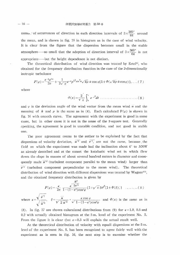
The theoretical distribution of wind direction was treated by ErteP>, who
obtained for the frequency distribution function in the case of the 2-dimensionally
isotropic turbulence
e -k p;;" 1 :;-3 • " - . - -F(cp) =-2·~+ 2 /-e-kp' sm '~'vkp u cos cp{l+ <P( vkp u coscp) }, .... ( 7)
~~ v r:
where
2 ~·' ., <,ti(x)=, 1 - e·'"dt ........................ (8) v 7r ()
and cp is the deviation angle of the wind vector from the mean wind u and the
meaning of k and p is the same as in (4). Each calculated F(cp) is shown in
fig. 16 with smooth curve. The agreement with the experiment is good in some
cases, but in other cases it is not in the sense of the X-square test. Generally
speaking, the agreement is good in unstable condition, and not good in stable
one.
The poor agreement :oeems to the author to be explained by the fact that
dispersions of velocity deviation, u"l and 17': are not the same, because . the
field on which the experiment was made had the inclination about 4" to NNvV
as already described and at the sunset the katabatic wind set in which flew
down the slope in masses of about several hundred meters in diameter and conse
quently made u'" (turbulent component parallel to the mean wind) larger than
1)1"-- (turbulent component perpendicular to the mean wind). The theoretical
distribution of wind direction with different dispersions was treated by W agner5;l,
and the obtained frequency distribution is given by
where
u'J " e- 2u'2 - ~ <2 ~ l
F(cp)=-- 1 (1 .,) . {l+J/rr,;-e·Cl+<i'(;L 1 ........ (9) 2rr - - ~e" cos· cp
.j v'" tr=---
• ._/ u'" ,
K COS '{J and <P(x) is the sa.me as in
(8). In fig. 17 are shown caluculated distributions from (9) for ~e = 1.0, 0.5 and
0.2 with actually obtained histogram at the 5 m. level of the experiment No. 5.
From the figure it is clear that ~e = 0.3 will explain the actual result well.
As the theoretical distribution of velocity with equall dispersions at the 5 m.
level of the experiment No. 5. has been recognized to agree fairly well with the
-experiment as is seen in fig. 16, the next step is to examine whether the


Fig. 17. Frequency distribution of wind direction for z=5 m., No. 5.
-27-
. 14
I. 2
.I 0
-0.8
Fig. 18. Frequency distribution of wind velocity for z=5 m., No. 5.
theoretical distribution of velocity with different dispersions for r.: =0.3 shows
only a slight c'.eviation from that of equal dispersions. The theoretical distribution
of wind velocity with different dispersions was aim deduced by Wagner as
follows:
V"(l--r.:") where 11=-- ----1. 2tt~ K'.!. '
'lt-v
uV !..1=~ and
u'" S,(x) = f,~ix) e-',
z 1/1 j,(y) being the
Bessel Function of the m-th order. Wagner gave values of S1, s~, S;,, S,, S",
Sa, S, and S10 for x=0~40 in a table. But the poor convergency in this case
of the series has made the author give up (10) c.nd calculate numerically by the
original formula
V )2" V" ( ( u \2 , _sin"£. } F(v ___ - 2 '" \_ COS<f?-v) T " . 1
)=zr:r.:u''' o e u " a~.p . .......... (11)
In fig. 18 are shown two theoretical curves, one for r.: = 1 calculated from
(2) and the other for r.:=0.3 obtained from (11), with experimentally obtained
histogram. Both curves show only a slight deviation from each other, and our
presumption that the disagreement in the frequency distribution in direction is
due to the unequalness of the dispersions seems to be confirmed.
Recently Koo"1) has deduced theoretical distributions of wind velocity and
direction taking into account the COlTelation between turbulent components of
wind. But to assume a correlation between u' and v' in our case is to accept
the predominance of a definite sense of the rotation of vortices with vertical

-28-
axes in the sudace layer which seems improbable, so it may be unnecessary to
consider the case with non-zero correlation.
(V) Coefficient of correlation
From the measured velocity two sorts of coefficient of correlation are
calculated --one is the coefficient of correlation (Ry or Ru;1, Zk) between
velocities at two points separated by y along the vertical and the other is the
coefficient of correlation (R,) between the velocity at a point and the velocity
at the same point but at time t later. Obtained values of Ry are shown after
the manner of SchrnidtHl as follows :
Values of Rttzt,U=~
(1) unstable, v;=3.47 m./~ec. (5) stable, V, = 2. 01m./sec.
5 0.868 5 0.713 2 0.816 0.821 0.781 2 0.430 0.188 0.653 1 0.876 0.756 1 0.433 0.538 0.5 0.5
(2) stable, Vo=2.69 m.h;ec. (6) unstable, V,, = 3. 7,1 m./sec.
5 0.627 5 0.803 2 0.235 0.363 0.561 2 0.789 0.732 0,6<14 1 0.400 0.458 1 0.670 0.710 0.5 0.5
(3) unstable, v-;=1.97 m./sec. (7) stable, V.,=2.89 m./sec.
5 0.772 5 0.662 2 0.693 2 0.649 1 0.813 0.659 0.685 1 0.731 0.57G 0.561
0.5 0.725 0.5 0.631
(4) stable, v;=4.01 m.(fec. (8) unstrcble, 1'.,=4.65 m./sec.
5 0.769 5 0.726 2 0.704 2 0.598 1 O.E46 0.697 0.638 1 0.598 0.798 0.658
0.5 0.738 0.5 0.678
For the sake of comparison values at the corresponding heights are extracted
from Schmidt's paper as foiiows:
Group I . V,=2.4 m./sec. Group H. V,=3.8 m./sec.
5 0.78 5 0.42 2 0.69 2 0.22 1 0.83 1 0.55
It is· interesting to note that, though instruments and time scales applied are
quite different in Schmidt's and our cases, magnitude of values are approximately
the same except in Schmidt's Group H where they are somewhat small.
Schmidt describes that values of the correlation coefficient decrease as the mean
velocity becomes large, but it is not clear in our case where the effect of
stability of the air layer seems to cover more the decrease.
It is clez.r in our case that values of the correlation coefficient become
smaii as the air layer becomes more stable, which explains the fact that the
air layer at different heights generaiiy tends to flow indepenently as the stability
becomes large. Shiotani also remarks that the instability of the air layer makes
the value of Ry larger.
-:2Cl-
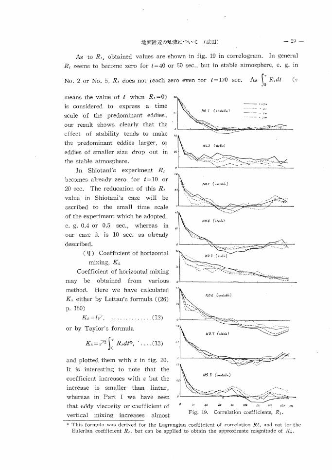
As to R,, obtainea values are shown in fig. 19 in correlogram. In general
R, seems to become zero for t=40 or SO sec., but in stable atmosphere, e. g. m
No.2 or No. 5, R, does not reach zero even for t=170 sec. As ~: R,dt (-r
means the value of t when R, =0)
is considered to express a time
scale o:f the predominant eddies,
our result shows clearly that the
effect of stability tends to make
the predominant eddies larger, or
eddies of smaller size drop out in
the stable atmosphere.
In Shiotani's experiment R,
b:=wmes already zero for t = 10 or
20 sec. The reducation of this R,
value in Shiotani's case will be
ascribed to the small time scale
of the experiment which he adopted,
e. g. 0.4 or 0.5 sec., whereas m
our case it is 10 sec. as already
described.
(VI) Coefficient of horizontal
mixing, K"
Coefficient of horizontal mixing
may be obtained from various
method. Here we have calculated
K"' either by Lettau's formula ( (26)
p. 180)
K~>.=lv', .............. (12)
or by Taylor's formula
_ 12 -K· • ( a -- ~T Kh-v 0 R,dt, .... ,lu)
and plotted them with z in fig. 20.
It is interesting to note that the
coefficient increases with z but the
increase is smaller than linear,
whereas in Part I we have seen
that eddy viscosity or coefficient of
vertical mixing increases almost
r.o
0 60 fo ,., Fig. 19. Correlation coefficients, R 1 •
* This formula was derived for the Lagrangian coefficient of correlation R~, and not for the Eulerian coefficient R 1 , but can be applied to obtain the approximate magnitude of II.,.

-30-
' .., /
"//f'/ . "' " • ~{o
0 ,. I • o sl:.bfe
0 !" 0 0 ('! • •n•!i.ble
I.
1 '
o;l; "'~
0 2 3 K,
( Lel:tau)
Fig. 20. Coefficient of horizontal mixing. Fig. 21. Coefficient of horizontal mixing calculated by Taylor's formula and Lettau's formula.
linearly with z.
In fig. 21 K" calcul2.ted by (12) is plotteo_ against K" cc:_lculaJec_ by (13).
From the figure it is seen that K;, ccJculatec_ by Lettau's formulc>. is smaiier by
about 30% than K" calculated by Taylor's formula, and es.pecidly in the stable
atmosphere.
§4. Summary
In view of the fact that published results on the irregelcx or turbulent
component of wind c.re only a few, the author describes his own experiment in
which following results c-cre found:
(1) The turbulent eno;rgy V7" increases with height, the rate of increase
being somewhat larger than lnz. The stratification of the air layer may have
some effect on the rate of increase but it is difficult to find out any law from
the experiment except that ec..ch value of energy itself becomes smaller with
stability.
(2) The relative intensity of turbulence / V' 3 j V. decreases with height.
The decrease is very steep in the layer near the ground but won becomes slight
or almost constant as the height increases.
(3) The frequency distribution of the vc.riation of wind velocity can be
explained fairly well by the Hesselberg anc_ Bjcrkdal's theory in which 2-
dimensional isotropy and normal distribution of components of the variation of
wind velocity are m:sumec ..
(4) The frequency distribution of the variation of wind direction can be
explained by Ertel's theory in ur1stable condition but not in stable one. This
may be due to the katabatic wind which flew down the field, and Wagner's.

-31-
theory with different di£persions pfoves to be in agreement with the results
both for wind direction and velocity.
(5) Two sorts of coefficient of correlation between velocities are calculated..
One, the coefficient between velocities at two points separated by y along the
vertical, is shown to decrease as the stability becomes large, and the other, the
coefficient between the velocity at a point and the velocity at the same point
but at time t later, seems to decrease with t more gradually to zero as the air
layer becomes more stable ; and probably this will explain the fact that the
effect of stability tends to make the predominant eddies larger or eddies of
smaller size drop out in the stable atmosphere.
(6) Coefficient of horizontal mixing are calculated both by Lettau's formula
and by Taylor's formula and it is £hown that the former gives about 30%
smaller values than the latter. The coefficient calculated by either of the two
formula seems to increm:e with z £maller than linear in cotrast to the almost
linear increase with z of eddy viscm:ity or coefficient of vertical mixing.
REFERENCES
1. Best, A. C. 1935 Transfer of heat and momentum in the lowest layers of the atmosphere,
Geophys. Mem. 65, 1-66.
2. Brunt, D. 1939 Physical and Dynamical Meteorology, 2nd ed.
3. Calder, K. L. 1949 The criterion of turbulence in a fluid of variable density, with
particular reference to conditions in the atmosphere, Q. ]. R. M. S. 75, 71-88.
4. Deacon, E. L. 1949 Vertical Diffusion in the Lowest Layers of the Atmosphere, Quart.
Journ .. Roy. Met. Soc. 75, 89-103.
5. Ertel, H. 1929 Die Richtungsschwankung der horizontalen Windkomponente in turb:.~lenten
Lurtstrom, Gerlands Beitr. z. Geophys. 23, 15-21.
6. Ertel, H. 1930 Eine Methode zur Berechung des Austauschkoeffizienten aus den
Feinregistrierungen der turbulenten Schwankungen, Gerlands Beitr. 25, 279.
7. Ertel, H. 1933 Beweis der Wilh. Schmidtschen konjugierten Potenzformeln fur Austausch
und Windgeschwindigkeit in den bodennahen Luftschichten, Met. Z. 50, 386-388.
8. Ertel, H. und Jaw, ]. ]. 1938 Uber die Bestimmung der Parameter im Verteilungsgesetz
turbulenter Windschwankungen, Met. Z. 55, 205-207.
9. Frankenberger, E. 1948 Uber den Austauschmechanismus der Bodenschicht und die
Abhangigkeit des vertikalen Massenaustausches vom Temperaturgefalle nach Untersuchungen
an den 70 m hohen Funkmasten in Quickborn I Holstein, Ann. der Met. Beiheft, 1-23.
9a. Frenkiel, F. N. 1951 Frequency distributions of velocities in turbulent flow, Journ.
Met 8, 316-320.
10. Giblett, M. A. 1932 The structure of wind over level country, Geophys. Mem. No. 54.
11. Halstead, N. H. 1951 The relation between wind structure and turbulence near the
ground, Supplement to Interim Report No. 14, Micrometeorology of the Surface Layer of
the Atmosphere, The Johns Hopkins University, Laboratory of Climatology, 1-48.
12. Hellmann, G. 1914 Uber die Bewegung der Luft in den untersten Schichten der

32-
Atmosphtire, Erste Mitteilung, Sitzungsber. Pr. Akad. Wiss. Berlin 415-437.
13. Hellmann, G. 1917a Zweite Mitteilung, Sitzungsber. Pr. Akad. Wiss. Berlin 174-197.
14. Hellmann, G. 1919 Dritte Mitteilung, Sitzungsber. Pr. Akad. Wiss. Berlin 404-416.
15. Hellmann, G. 1915 Uber die Bewegung der Luft in den untersten Schichten der
Atmosph:'ire, Met. Z. 32, 1-16.
16. Hellmann, G, 1917b Zweite Mitteilung, Met. Z. 34, 273-285.
17. Hesselberg, von Th. und Bjorkdal, E. 1929 Uber das Verteilungsgesetz der Windunruhe,
Beitr. Phys. fr. Atm. 15, 121.
18. Heywood, G. S. P. 1931 Wind structure near the ground and its relation to temperature
gradient, Quart. ]ourn. Roy. Met. Soc. 57, 433-455.
19. Karmim, Th. von 1937 The fundamentals of the statistical theory of turbulence, ]ourn.
Aero. Sci., 4, 131-138.
20. Kawahara, T. 1950 Some Problems in the Lowest Layer of the Atmosphere, Bull.
Fuculty of Agric. Mie University, No. 1, 45-53.
21. Koo, C. C. 1945 The general laws of frequency distribution of wind in a gust, Mem.
Nat. Res. Inst. Met. Aca:i. Sinica, 14, 1-15.
22. Lettau, H. und Schwertfeger, 1933 V ertikalaustausch in unmittelbarer, Berechnung, lVIet.
z. 50, 47.
23. Lettau, H. unp Schwertfeger, 1933 Untersuchungen tiber atmospharische Turbulenz und
Vertikalausch vom Freiballon aus, 1ste Mitteilung, Met. Z. 50, 250.
24. Lettau, H. und Schwertfeger, 1934 Untersuchungen tiber atmospharische Turbulenz und
Vertikalaustausch vom Freiballon aus, 2te Mitteilung, Met. Z. 51, 249.
25. Lettau, H. und Schwertfeger, 1936 Untersuchungen tiber atmospharische Turbulenz und
Vertikalaustausch vom Freiballon aus, 3te Mitteilung, Met. Z. 53, 44.
26. Lettau, H. 1930 Atmospharische Turbulenz.
27. Lettau, H. 1949 Isotropic and Non-Isotropic Turbulence in the Atmospheric Surface
Layer, Geophys. Res. Pap. No. 1, Cambridge, Mass.
28. Paeschke, W. 1937 Experimentelle Untersuchungen zum Rauhigkeits· und Stabilitiitspro·
blem in der bodennahen Luftschicht. Beitr. z. Phys. fr. Atm. 24, 163.
29. Pasquill, F. 1949a Eddy Diffusion of Water Vapour and Heat near the Ground, Proc.
Roc. Soc. 198, 116-140.
30. Pasquill, F. 1949b Some estimates of the amount and diurnal variation of evaporation
from a clayland pasture in fair spring weather, Q. ]. R. M. S. 75, 249-256.
31. Prandtl, L. 1932 Meteorologische Anwendung der Stromungslehre, Beitr. z. Phys. fr.
Atm. 19, 188-202.
32. Rossby, C. G. and Montgomery, R. B. 1935 The layer of frictioml influence in wind
and ocean currents, Papers in Phys. Ocean. Met. 3, No. 3.
33. Rossby, C. G. 1926 The vertical distribution of atmospheric eddy energy, Month. Weath.
Rev. 54, 321-332.
34. Schmidt, W. 1935 Turbulence near the ground, ]ourn. Aero. Soc. 39, 355.
35. Scrase, F. ]. 1930 Some characteristics of eddy motion in the atmosphere, Geophys.
Mem. No. 52.
36. Shiotani, M. and Yamamoto, G. 1946 Atmospheric turbulence over the large city, 1st
Report, ]ourn. Met. Soc. Japan 27, 111-115.
37. Shiotani, M. 1950 Turbulence in the lowest layers of the atmosphere, Sci. Rep. Tohoku

-33-
University, Ser. 5, Geophys. 2, No. 3, 167-201.
38. Sutton, 0. G. 1936 The Logarithmic Law of Wind Structure near the Ground, Quart.
Journ. Roy. Met. Soc. 62, 124-127.
39. Sutton, 0. G. 1937 The Logarithmic Law of Wind Structure near the Ground, Quart.
Journ. Roy. Met. Soc. 63, 105-107.
40. Sutton, 0. G. 1949a The application to micrometeorology of the theory of turbulent
flow over rough surfaces, Quart. Journ. Roy. Met. Soc. 75, 335-350.
41. Sutton, 0. G. 1949b Atmospheric turbulence.
42. Sverdrup, H. U. 1936 The eddy conductivity of the air over a smooth sno>viield,
Geofysiske Pub!. 11, No. 7, 1-69.
43. Sverdrup, H. U. 1936 Note on the Logarithmic Law of Wind Structure near the Ground,
Quart. Journ. Roy. Met. Soc. 62, 461-462.
44. Sverdrup, H. U. 1939 Second Note on the Logarithmic Law of Wind Structure near the
Ground, Quart. Journ. Roy. Met. Soc. 65, 57.
45. Takeda, K. 1949 On the atmospheric Turbulence, 1st Paper. Journ. Met. Soc. Japan,
27, 333-341, 363-370.
46. Takeda. K. 1951 On the atmospheric Turbulence, 2nd Paper, Journ. Met. Soc. japan,
29, 233-245.
47. Takeda, K. 1951 On the Atmospheric Turbulence, 3rd Paper, Journ. Met. Soc. Japan
29, 287-297.
48. Takeda, K. 1952 On the Atmospheric Turbulence, 4th Paper, Journ. Met. Soc. Japan,
30, 141-146.
49. Takeda, K. 1952 On the vertical air temperature distribution in the lowest layers of
the atmosphere, ]ourn. Agric. Met. 7, 1-3. in Japanese, with English Resume.
50. Taylor, G. I. 1918 Phenomena connected with turbulence in the lower atmosphere, Proc.
Roy. Soc. 94, 137.
51. Thornthwaite, C. W. and Halstead, M. 1942 Note on the Variation of Wind with Height
in the Layer near the Ground, Trans. Amer. Geophys. Union, Part. li 249-255.
52. Thornthwaite, C. W. and Holzman, B. 1939 The determination of Evaporation from Land
and Water Surface, Month. Weath Rev. 67, 4-11.
53. Thornthwaite, C. vV. and Holzman, B. 1942 Measurement of Evaporation from Land and
Water Surface, U. S. Dept. Agriculture, Techn. Bull. No. 817, 75 pp.
54. Thornthwaite, C. W. and Paul, 1943 Wind Gradient Observations, Trans. Amer. Geophys.
Union, Part. I. 166-182.
55. Wagner, A. 1929/30 Theorie der Biiigkeit und Haufigkeitsverteilung von Windstiirke
und Windrichtung, Gerlands Beitr. z. Geophys. 24, 386-436.

- 34 ー 林業試験場研究報告第 58 号
地面附近の乱流について
武 田 -口小
森林に対する風寄p 防風林或は森林火災の研究は近年汗しく進歩しつ L あるが,そ tわ研究及
び、対策には.il'_均風速のみなら-t-胤のもつí1tZ't ,イ9:] え(王子l~J}!!\UiliのJïi; uï分イIj, J瓜の乱JU手も考!告:
される様になった。
然しその為には子千々は〉じ十~j{:等J) }!!\~の~!Y'I"I:l'tを l切らかにしてゐ〈必要がある。以下かつて著
者ーの行った実験及び、他の主子封切実験を誌としてJÜ!.ll'rî附;庄の J.!li_~の性'Cf を訓べるととにする。
地問間近の風の性ftの研究には_:j~の竺組 1) の方法が5jうーえられる。
1) JÆ~命(I'Jjjylミ
尤もらしい),t碓似定から 11',発して '1三五J)9i.l:iι 乱~LJコ垂直分布その他を導11',するもの,現在迄
に浩子の;試みがなされているが, fl 下孔ìfrUlJl論そのものが:{!;i2iな発注の段併にあるので気後へ
の応川は未だしの感があり,一方従来の正'11諭は新しい乱ifrCllJ日1討の立場からはると組めて不十分
なものとはられる υ
2) 実験(I';j方法(ー〉
千五j風iiliの~直分不fj を)jくめそれからよく 5,11 られた関係式をJiJ いて担介距離, ~NI)勤もIj'!生係数等
を導11',しようとするもの,との方法で、は.L1'- :t::J風辿の表直分布を川来るだけ IE確に 5,11 る必要があ
る。然し-"1三J~J風速のìJ!1!jCは比較的存易で、あるから従来多くの人によって試みられて来たc
3) 実験(I'~方法(二〉
).!li_~の変動の主也うよギliの ìJlI!定から風の他の↑'tfT を調べんとする方法。とのブj訟は制めて興味の
ある J;法ではあるが胤の変動のì!lIJjCは本易でないので余り行われてし、ない。
本報告の目的
現在のf円安当とJEわれる理論を展P;Jするととが困難であったので主として実験的方法に依っ
た。本報告の第一部に於いては平均風速垂直分布の問題を取扱い従来の多くの著者(現著者を
も合む)の実験的並び、に王里論的研究を総括しp 最も信頼するに足ると,巴われる平均風速の垂直
分布の式を提出する。そして之を IIJ~ 、て混合距離,渦動粘性係数,蒸発公式等を取扱う弘。菜二
部lに乙於いては反風Lの変動iに乙関する l川J日川1りj陪題を J取1!Z元!Zi扱及う九。 i但旦し!風E孔Lの変動に関するi司訓別洲!l知則II羽1];定11ιi立:誠品訓t私判Il同I
tれLていないのでで、著者.官白身の観i訟別洲Jl却則11羽1)結斗巣Lについて迷べ,特に安定度との諸関係を l切らかならしめんJ
とした。

地面附近の乱流について (武田) • 35 -
結果
U~~1Jm
1) 111f然 J(気 'j_t に }j~' \,、ては 7f,'んど総;てのJ:M合;こ
u~IIZZ
の~fI iき)!!i\のか{l î式を11"'川すれば十分で、あること,ス実験(粗1芝の附近lこ於ける)がとのうトギlîか
ら!日怖を生やる場合に於いてのみ
u~ln(z士 d)
を fR川寸ればよいととが示された。
2) 粗度の夫げ吋IÎに U於-いて 1μt が実詞i際漂の胆風u辺辿1止fに芋しくなる立如如I日lパ< rlL日"暗i
度と j共=に変るととが三示了戸:さ AれLた。即ち簡単な対数法j[lJ
zt= alll_3-Z ,)
が咋川されるならばんは安定度と!~に増えする。 31i し対数法[(IJからの íl]1奇を夫わず法JilJが探
川されるならば ZI)は安定度と jGにi成少する。 そして多分この方が実際であろうと,Uわれる。
3) Deacon の析しい分布式r[ tのベラメーター σ 及びそれから件られる ìl,',\動 *M"f:係数 K の
式は机りであるととが示され,訂正された.J.:tがHH l't された。
4) ;if I[ された K の式を使川すると PasquiIIの実験に於いて K=K" (氷蒸気l乙対する
ìr\',\!ûJJ依 1\)(1系数)を実験的l乙示すととが/1 1来る。 (PasquiII は Deacon の北Ii'tした K の式を
使った為それが/1',来なかった)。
5) 現在の所 Deacon の辿度分'1Iî :rt
u=~( Zl-ß--zl一町1-丘、
がilk も簡単で、 LLつ実験IL~はもよく迎合すると考えられる。(但しれは Deacon とは~~なり安
定皮によって変わる。.fl[Jち安定!立と共に減少すると rJ える〉。 そして以後の考肢の jえ礎式に侃
JIJ さ ~Lる。
6) Deacon の分布式をJ弔問すると混合距離及び渦到桁性係数は火の立/1くなる。
1 =0.4 h(ß) 日z
及び K=O.4v
ととで安定l度のみによって変ると考えられるバラメータ - h は Pm:quil1の実験から求め
ら ÆLる。
7) v-xJU の安定度iこ対する変化を Pasquill の実験から求めた所 Ri=O で版小となった。
との結県は少し奇妙なもの L お1 C\ιわれるので将来更に他の資料に就いて検討する必要があろ
つ。

- 36 林業試験場研究報官第 58 号
8 )上に定義されたパラメータ - h(ß) は Thornthwaite の蒸発公式中にも生やるととが
示された。そして大きな n'lì1'/tから正確な蒸発長を求める Thornthwaite の方法はゴ1"断熱ん気
の場合には h(ß) が他の )j法例えば'f[)或は気温と町射長tr(j,から求められない以上;也JIJ し仰な
いととが注意された。
弟二部
J_ílllの変動成分に関する発火された幸1!IJl~は少いので非J計自身の実験に就いて症べる。 Nられた
がU!~!主 c:J(の主fIくである。
1 )乱流エネルギー V" はめij[Jtと共に増大する。増大の在IJ0-は lnz よりは幾ー分んである。
気祖の垂直分布の影響は,エネルギーの値自身が安心 I:.気 'i' でノj、さくなる以外には,実験から
は明瞭でなカ込つた。
2 )乱
i税}}段!宝tでで、あるがP 高さとjbにむきに絞但或は殆んど-Æとなる。
3) 風速変動の頻度分布は変到J成分の二次元等ブ(pl"I:及び TEJJ~分布を仮定した Hesselberg 及
び、 Bjδrkdal の五I[論によって11JJ点りよく首主明される。
4) 風向変動の頻度分布は不安定条件の場合には Ertel の型H論でよく設rlfj出来るが, 安定
条例ーの場合には説明 11 ',来ない。之はその i療に千子在したカタパJ!lilの為であると考えられる。そし
て方向によって異なれる分・散をもった Wagner の正弘前がJ!liU!!Ui'.びに風Ii~Jの結果をよく ri}t l リjす
るととが示された。
5 )風辿変動成分の 1111の二抑制の相関係数 Ry 及び、 R, が求められた。垂直方向に y だけ
p日った二点l乙於ける辿!主成分のIiI1の相関係数 Ry I土 'k'~tË l支がI??すと共に ii安少する。 之は安定
J:.気 çl'では上下の5:~気 11せがjミ々独立に流れようとする何i[i'iJ を示すものであろう。又~,I.I~~に於け
る辿度と同じ点に於けるH寺1111 t 後の;主度との間の+íl関係数 Rt は t と ~f~に減少するが,安定
大気の場合iこはその減少がより絞慢である。そして之は多分安定大気 II~で、は卓越するか肋:大き
くなる,或はノj、さな )f,i,\iJ '打JV)えする事を ;&1珂するものであろう。
6) 7](千拡散ーの係数が Lett正lU及び Taylor の tj法によって求められた。そして前Jfの方が
後者ーより約 3096 小さな値を与えるととが示された。イi'.fAlの方法によるも求められた係数は高
度に対して也料的問には貯えしないととが認められる(之に対してH,'日古川住係数或は垂直;拡散
の係数!幻':jl1[と共に殆んど、直線(I'~に J('ì:lくする)。