James Bridges and Mark P. WernetGlenn Research Center, Cleveland, Ohio

Turbulence Measurements of Separate FlowNozzles With Mixing Enhancement Features

NASA/TM—2002-211592

June 2002

AIAA–2002–2484

https://ntrs.nasa.gov/search.jsp?R=20020083021 2020-04-28T07:32:14+00:00Z

The NASA STI Program Office . . . in Profile

Since its founding, NASA has been dedicated tothe advancement of aeronautics and spacescience. The NASA Scientific and TechnicalInformation (STI) Program Office plays a key partin helping NASA maintain this important role.

The NASA STI Program Office is operated byLangley Research Center, the Lead Center forNASA’s scientific and technical information. TheNASA STI Program Office provides access to theNASA STI Database, the largest collection ofaeronautical and space science STI in the world.The Program Office is also NASA’s institutionalmechanism for disseminating the results of itsresearch and development activities. These resultsare published by NASA in the NASA STI ReportSeries, which includes the following report types:

• TECHNICAL PUBLICATION. Reports ofcompleted research or a major significantphase of research that present the results ofNASA programs and include extensive dataor theoretical analysis. Includes compilationsof significant scientific and technical data andinformation deemed to be of continuingreference value. NASA’s counterpart of peer-reviewed formal professional papers buthas less stringent limitations on manuscriptlength and extent of graphic presentations.

• TECHNICAL MEMORANDUM. Scientificand technical findings that are preliminary orof specialized interest, e.g., quick releasereports, working papers, and bibliographiesthat contain minimal annotation. Does notcontain extensive analysis.

• CONTRACTOR REPORT. Scientific andtechnical findings by NASA-sponsoredcontractors and grantees.

• CONFERENCE PUBLICATION. Collectedpapers from scientific and technicalconferences, symposia, seminars, or othermeetings sponsored or cosponsored byNASA.

• SPECIAL PUBLICATION. Scientific,technical, or historical information fromNASA programs, projects, and missions,often concerned with subjects havingsubstantial public interest.

• TECHNICAL TRANSLATION. English-language translations of foreign scientificand technical material pertinent to NASA’smission.

Specialized services that complement the STIProgram Office’s diverse offerings includecreating custom thesauri, building customizeddata bases, organizing and publishing researchresults . . . even providing videos.

For more information about the NASA STIProgram Office, see the following:

• Access the NASA STI Program Home Pageat http://www.sti.nasa.gov

• E-mail your question via the Internet tohelp@sti.nasa.gov

• Fax your question to the NASA AccessHelp Desk at 301–621–0134

• Telephone the NASA Access Help Desk at301–621–0390

• Write to: NASA Access Help Desk NASA Center for AeroSpace Information 7121 Standard Drive Hanover, MD 21076

James Bridges and Mark P. WernetGlenn Research Center, Cleveland, Ohio

Turbulence Measurements of Separate FlowNozzles With Mixing Enhancement Features

NASA/TM—2002-211592

June 2002

National Aeronautics andSpace Administration

Glenn Research Center

Prepared for theEighth Aeroacoustics Conferencecosponsored by the American Institute of Aeronautics and Astronauticsand the Confederation of European Aerospace SocietiesBreckenridge, Colorado, June 17–19, 2002

AIAA–2002–2484

Acknowledgments

This work was supported by NASA Supersonic Propulsion Base Research program under Mary Jo Long-Davis.The authors thank Dr. Abbas Khavaran for his consultation on the turbulence modeling and aeroacoustic theory.

Available from

NASA Center for Aerospace Information7121 Standard DriveHanover, MD 21076

National Technical Information Service5285 Port Royal RoadSpringfield, VA 22100

This report is a preprint of a paper intended for presentation at a conference. Becauseof changes that may be made before formal publication, this preprint is made

available with the understanding that it will not be cited or reproduced without thepermission of the author.

Trade names or manufacturers’ names are used in this report foridentification only. This usage does not constitute an officialendorsement, either expressed or implied, by the National

Aeronautics and Space Administration.

Available electronically at http://gltrs.grc.nasa.gov/GLTRS

NASA/TM2002-211592 1 American Institute of Aeronautics and Astronautics

Turbulence Measurements of Separate Flow Nozzles with Mixing Enhancement Features James Bridges* and Mark P. Wernet*

National Aeronautics and Space Administration Glenn Research Center Cleveland, Ohio 44135

Abstract

Comparison of turbulence data taken in three separate flow nozzles, two with mixing enhancement features on their core nozzle, shows how the mixing enhancement features modify turbulence to reduce jet noise. The three nozzles measured were the baseline axisymmetric nozzle 3BB, the alternating chevron nozzle, 3A12B, with 6-fold symmetry, and the flipper tab nozzle 3T24B also with 6-fold symmetry. The data presented show the differences in turbulence characteristics produced by the geometric differences in the nozzles, with emphasis on those characteristics of inter-est in jet noise. Among the significant findings: the enhanced mixing devices reduce turbulence in the jet mixing region while increasing it in the fan/core shear layer, the ratios of turbulence components are significantly altered by the mixing devices, and the integral lengthscales do not conform to any turbulence model yet proposed. These find-ings should provide guidance for modeling the statistical properties of turbulence to improve jet noise prediction.

Introduction

In 1997, as a part of NASA’s Advanced Subsonic Technology Program, a series of separate flow nozzle concepts were tested. Concepts based upon the para-digm of noise reduction through mixing enhancement were submitted by General Electric Aircraft Company, Pratt &Whitney, and Rolls Royce Corporation. Several of these nozzle concepts provided significant noise benefits with negligible thrust penalty. During the 1997 Separate Flow Nozzle Test (SFNT), many measure-ments were made on the jet flows: far-field acoustics, total and static pressure and total temperature surveys of the plume, infrared imagery of the plume, acoustic source distribution estimation by phased arrays, and Schlieren images1. These combined to describe the mean flow field and acoustic fields for the jet flows, leading to some understanding of how changes in the flow field caused beneficial changes in the acoustic sources.

As successful as the 1997 SFNT was, one key class of information was not acquired: turbulence statistics are the main information that aeroacoustic theory requires to relate flow to sound. Specifically, leading theories require two-point space-time correlations of the veloc-ity field as input to predict acoustic output of the jet flow. A second series of tests were performed in 2000 using the SFNT test hardware, the test being called SFNT2K. The datasets for the separate flow nozzle tests now have turbulence measurements, including two-point space correlations, for the three most impor-tant nozzle configurations.

Facilities and Instrumentation

The AST Separate Flow Nozzle Tests were conducted at the AeroAcoustic Propulsion Laboratory (AAPL) at NASA Glenn Research Center in Cleveland, Ohio. The

exhaust nozzle models were mounted on a hydrogen-fired jet engine exhaust simulator rig inside a freejet, providing a scaled model of engine nozzles at appropri-ate hot flow conditions in simulated flight.

The Aeroacoustic Propulsion Laboratory (AAPL) at NASA Glenn Research Center is a 65ft radius, anech-oic, geodesic dome. Within the acoustically lined con-fines of the dome is the Nozzle Acoustic Test Rig (NATR), a free-jet, forward-flight-simulation test rig. The NATR extends from an annular air ejector system to a plenum and bellmouth contracting down to the fi-nal duct having an exit inner diameter of 53 inches and a nozzle centerline 10 feet above the concrete floor. This arrangement provides a free-jet Mach number up to 0.3 at 300 lbm/s with the freestream turbulence of less than 1 percent2.

Test nozzle models are installed on the aft end of the hydrogen-fired jet exit rig (JER) that is located at the exit of the NATR duct. The core stream of the rig was used to provide the hot core flow, while the fan flow came from a secondary strut into a dual flow ‘pod’ fas-tened just aft of the combustor. For the PIV measure-ments, a choke plate replaced the reticulated foam metal to keep seed from clogging and destroying the foam metal.

Mass flow was measured using a choked-flow venturi located in the 4" supply lines downstream of the fan/core flow split, in the long horizontal pipe runs alongside NATR. Two total pressure and two total tem-perature rakes (with five elements each) were installed at the charging station of the fan and of the core ducts of the dual flow pod. The fan rakes are installed at circumferential angle positions of 0°, 90°, 180°, and 270°, while core nozzle rakes are located at circumfer-ential angles of 60°, 150°, 240°, and 330°.

In these tests, the core and bypass streams were seeded with aluminum oxide (Al2O3) powder using two identi-cal, specially built, fluidized bed seeders. The alumina powder had a specific gravity of 3.96; the *AIAA Senior Member.

NASA/TM2002-211592 2 American Institute of Aeronautics and Astronautics

particle size distribution had a mean of 0.7 µm and a standard deviation of 0.2 µm. The seeders provided roughly 0.5liters/hour of dry seed particles each, seed-ing the flow at a rate of ~10 particles/mm3. Given the light sheet thickness of 0.2mm, this produces on the order of 10 particles in a 2mm by 2mm interrogation region. The ambient flow was seeded by a commercial fogger, Vicount 5000, manufactured by Corona Tech-nologies, Inc. This fogger produced droplets in the 0.2-0.3 micron diameter range at a rate of 5 liters/hour of fluid.

The PIV system was a two-camera system configured to yield two image fields, one above another with a slight overlap. The two 1K×1K pixel Kodak ES 10 cameras equipped with f/5.6, 85 mm Nikkor lenses and 8mm extension rings were mounted one atop the other 52 inches (1.32m) away from the light sheet. The two cameras were positioned to overlap their fields of view by 0.5 inches, yielding a composite field of view 10.5 inches high by 5 inches wide (0.267m x 0.127m). A dual head Nd:YAG laser operating at 532 nm was used to generate a 400 mJ/pulse light sheet. The laser, cam-eras, and all laser optics were mounted on a large axial traverse. Radial planes were measured in different circumferential angles by rotating the nozzle on the jet rig. Figure 1 shows the traverse positioned in an up-stream location with the PIV system operational.

The laser pulses were synchronized with the cameras and frame-grabbers using TSI Corporation's Insight (Version 3.2) software and Synchronizer. The Synchro-nizer controlled the timing of the pulsed light source relative to the CCD camera frame transfer period. PIV image frame pairs, required to produce an instantaneous velocity map, were acquired primarily at a time separa-tion of 2.2 microseconds. This was done to accommo-date the expected out of plane motion, instantaneously as high as 150m/s, with a light sheet 0.6mm thick. Pre-vious experience with PIV in jets showed that out of plane motion was a limiting factor in obtaining accurate results. To test this understanding, limited data points were acquired with 4 and 6 microsecond pulse. The data processed at these time separation showed little difference in their turbulence statistics, but did have regions where the image correlation began to fail, signi-fying that out of plane motions were becoming impor-tant as the time separation become too long. At each location 400 image pairs were recorded by each cam-era.

The collected PIV image data were processed using a NASA-developed code. The PIVPROC software uses fuzzy logic data validation to ensure that high quality velocity vector maps are obtained3. The correlation based processing allows subregion image shifting, asymmetric subregion sizes and multi-pass correlation processing. A grid was constructed, registered on the nozzle lip from the first frame image, so that velocities computed from each image would create a uniform

map. Five velocity grid cells overlapped in the radial direction and three in the axial direction. A multipass scheme was employed, using first a 64 by 64 pixel re-gion to determine mean shift of images, followed by a 32 by 32 pixel pass with 50% overlap between grid cells. The 32 by 32 pixel grid corresponded to a 0.088 inch (2.24mm) grid size in physical space.

The procedure for computing statistics from a series of processed PIV image velocity vector maps utilizes sev-eral acceptance criteria to qualify vectors and identify and remove incorrect vectors: signal to noise ratios for the image correlation, hard velocity cutoff limits and an Chauvenay criteria procedure for identifying outliers. A relative data 'quality' metric was defined as the number of accepted velocity vectors at a point relative to the total number of frame pairs processed. This field was used to blank out regions of the contour plots where the quality was less than 0.8; most regions had a quality metric in the 0.90–0.99 range.

Test Models

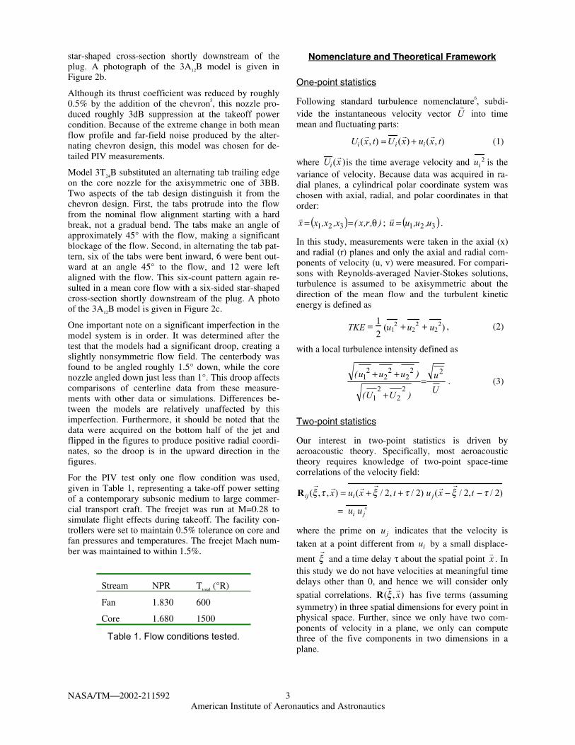
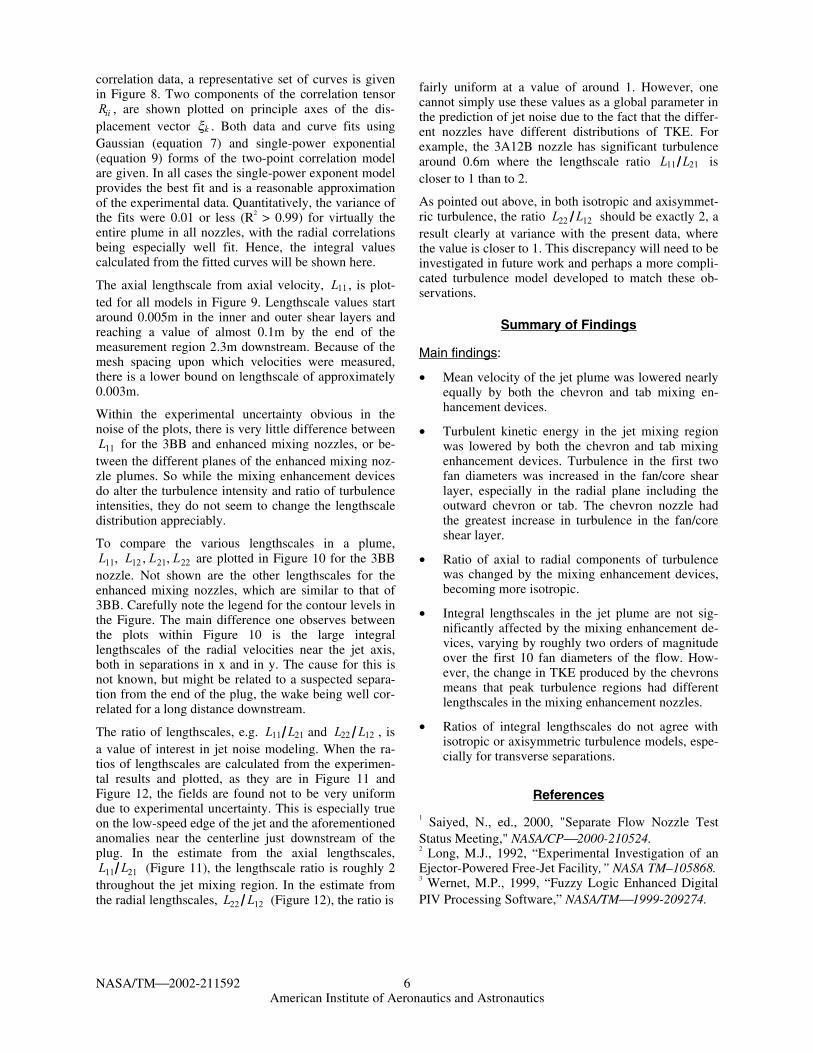
In the PIV portion of the SFNT2K test covered in this report, three nozzles were measured in detail. All noz-zles had bypass ratio 5 and an external plug. These were the baseline (3BB), alternating 12 count chevron (3A12B), and 24 count alternating tabbed nozzle (3T24B). These were chosen because they had the most dramatic and beneficial acoustic and mean flow changes as measured during the 1997 tests.

Model 3BB was the baseline nozzle, being axisymmet-ric on both core and fan nozzles. This model repre-sented a generic separate flow nozzle such as are flying on medium twin engine commercial transports today. The plug angle is approximately 16°. The core cowl exit diameter is 5.156 inches (130.9mm) (cold) and the core cowl external boattail angle is approximately 14°. At cold conditions, the core cowl exit plane is 4.267 inches (108.4mm) downstream of the fan nozzle exit plane. The fan nozzle had an exit diameter of 9.70 inches (246.3mm). A photo of this model is given in Figure 2a.

Model 3A12B substituted an alternating chevron trailing edge on the core nozzle for the axisymmetric one of 3BB. Chevrons can be thought of as being cut into the otherwise axisymmetric nozzle to have the baseline throat at the half height of the chevrons. Basic chevrons follow flow lines of baseline nozzle past the throat. The alternating chevron core starts from a flow–aligned chevron design with half of the chevrons being bent into the core stream approximately 4.5° with a small additional cusp to the chevron. The other half of the chevrons were bent into the fan stream by roughly 8°. More details about the original design philosophy and acoustic performance are given in reference 4, the report on the 1997 SFNT generated by GEAE, the designers of this nozzle. The result is a core flow with a six-sided

NASA/TM2002-211592 3 American Institute of Aeronautics and Astronautics

star-shaped cross-section shortly downstream of the plug. A photograph of the 3A12B model is given in Figure 2b.

Although its thrust coefficient was reduced by roughly 0.5% by the addition of the chevron5, this nozzle pro-duced roughly 3dB suppression at the takeoff power condition. Because of the extreme change in both mean flow profile and far-field noise produced by the alter-nating chevron design, this model was chosen for de-tailed PIV measurements.

Model 3T24B substituted an alternating tab trailing edge on the core nozzle for the axisymmetric one of 3BB. Two aspects of the tab design distinguish it from the chevron design. First, the tabs protrude into the flow from the nominal flow alignment starting with a hard break, not a gradual bend. The tabs make an angle of approximately 45° with the flow, making a significant blockage of the flow. Second, in alternating the tab pat-tern, six of the tabs were bent inward, 6 were bent out-ward at an angle 45° to the flow, and 12 were left aligned with the flow. This six-count pattern again re-sulted in a mean core flow with a six-sided star-shaped cross-section shortly downstream of the plug. A photo of the 3A12B model is given in Figure 2c.

One important note on a significant imperfection in the model system is in order. It was determined after the test that the models had a significant droop, creating a slightly nonsymmetric flow field. The centerbody was found to be angled roughly 1.5° down, while the core nozzle angled down just less than 1°. This droop affects comparisons of centerline data from these measure-ments with other data or simulations. Differences be-tween the models are relatively unaffected by this imperfection. Furthermore, it should be noted that the data were acquired on the bottom half of the jet and flipped in the figures to produce positive radial coordi-nates, so the droop is in the upward direction in the figures.

For the PIV test only one flow condition was used, given in Table 1, representing a take-off power setting of a contemporary subsonic medium to large commer-cial transport craft. The freejet was run at M=0.28 to simulate flight effects during takeoff. The facility con-trollers were set to maintain 0.5% tolerance on core and fan pressures and temperatures. The freejet Mach num-ber was maintained to within 1.5%.

Stream NPR Ttotal (°R)

Fan 1.830 600

Core 1.680 1500

Table 1. Flow conditions tested.

Nomenclature and Theoretical Framework

One-point statistics

Following standard turbulence nomenclature6, subdi-vide the instantaneous velocity vector

r U into time

mean and fluctuating parts:

Ui (r x , t) = Ui (

r x ) + ui (

r x , t) (1)

where Ui (r x )is the time average velocity and ui

2 is the variance of velocity. Because data was acquired in ra-dial planes, a cylindrical polar coordinate system was chosen with axial, radial, and polar coordinates in that order:

( ) ),r,x(x,x,xx θ== 321v

; ( )321 u,u,uu =v.

In this study, measurements were taken in the axial (x) and radial (r) planes and only the axial and radial com-ponents of velocity (u, v) were measured. For compari-sons with Reynolds-averaged Navier-Stokes solutions, turbulence is assumed to be axisymmetric about the direction of the mean flow and the turbulent kinetic energy is defined as

TKE = 12

(u12 + u2

2 + u22) , (2)

with a local turbulence intensity defined as

U

u

)UU(

)uuu( 2

22

21

22

22

21 =

+

++. (3)

Two-point statistics

Our interest in two-point statistics is driven by aeroacoustic theory. Specifically, most aeroacoustic theory requires knowledge of two-point space-time correlations of the velocity field:

R ij (r ξ ,τ ,

r x ) = ui (

r x +

r ξ / 2, t + τ / 2) uj (

r x −

r ξ / 2,t − τ / 2)

= ui u j'

where the prime on u j indicates that the velocity is

taken at a point different from ui by a small displace-

ment r ξ and a time delay τ about the spatial point

v x . In

this study we do not have velocities at meaningful time delays other than 0, and hence we will consider only

spatial correlations. R(r ξ ,

r x ) has five terms (assuming

symmetry) in three spatial dimensions for every point in physical space. Further, since we only have two com-ponents of velocity in a plane, we only can compute three of the five components in two dimensions in a plane.

NASA/TM2002-211592 4 American Institute of Aeronautics and Astronautics

The correlation is normalized in our data by the refer-ence variances,

22

R

ji

jiij

uu

'uu)x,(

~ =ξrv

. (5)

As a check, the correlations were also normalized by the local variances, with little difference in the result. This is one indication that the assumption of local ho-mogeneity was justified.

Models for Two-Point Correlations

Models for two-point correlations have traditionally been developed by assuming a functional form separa-ble in space and time. From the equations of motion certain constraints apply7:

uiu j ' = Rij (r ξ )g(τ)

Rij (r ξ ) = u1

2 f +ξf '2

δ ij −

f ' ξiξ j

2ξ

, f ' =

∂f

∂ξ

(6)

A popular analytic model for the two-point spatial cor-relation is the Gaussian form

2

2

Le)(f

πξ−

=ξ , (7)

yielding the models

( )

( ) 2

2

2

23

212

122

2

2

2

23

222

111

1

1

L

L

eL

uR

;eL

uR

πξ−

πξ−

πξ+πξ−=ξ

πξ+πξ−=ξ

(8)

When compared against current data, the Gaussian form seems a poor fit—the zero derivative of the correlation at ξ = 0 is not obvious and the curvature there is very small given the relatively large Reynolds number. Modifying the model above by changing the power of the exponent, setting

Le)(f

πξ−

=ξ (9)

produces a more satisfying fit to the data.

Another part of the popular model that does not agree with data is the assumption of isotropy. Indeed, it has been found that the two cross-stream turbulence intensi-ties are nearly equal, but are less than the axial turbu-lence intensity. For this reason an axisymmetric

turbulence model is examined. Following the deriva-tion8 and substituting a single-power exponential form for the Gaussian form, the two-point spatial correlation model is given by

( )( )

( )

( )( )))

23

22

21

22

1

2

2

22

23

22

21

21

21

222

22

23

22

21

21

21

1

123

222

223

23

22

2222

12

223

222

32111

2

44

1

1428

22

12

ξ+ξ+ξ∆=γ=∆ξγ

π=Χ

−=

−=

γΧ+Χ∆π+γ−Χ+

Χ

∆+−+

∆+−πγπ+∆γ−γΧπ+γ+

Χπ+=ξ

Χ−Χ−−=ξ

ξ+ξ+

ξπ−

ξ+ξ+

ξπ−

;K

K;

K

euuQ

;eu

Q

QK

K)(

Q)(R

Q)(R

ii

KK

KK

r

r

(10)

This is the functional form to which the data was fitted and to which it had the best fit.

Integral Lengthscales

In modeling the two-point spatial velocity correlation, it is often assumed that there is some displacement over which the velocities become uncorrelated. One defini-tion of this is the integral lengthscale L,

Lik(r x ) = ˜ R ii (ξk ,

r x ) dξk

0

∞

∫ , (11)

which happens to nicely match the scaling exponent L of the Gaussian form. One can still apply the same definition for lengthscale L to cases where the flow is not isotropic. However, computing this integral with discrete data over a finite range, such as is obtained in the present experiments, does introduce a significant uncertainty in the measure of L. Fitting a reasonable functional form to the data and integrating it yields a statistic independent of interrogation region.

One nice property about integral lengthscales is the ratio of Lii Lki = 2, i ≠ k for isotropic turbulence. Even in axisymmetric turbulence, the ratio still holds when i = 2 or 3 and k = 1. That is, when the separation vector is cross-stream, the correlation of axial velocity should decay at twice the rate of the velocity component in the separation direction.

NASA/TM2002-211592 5 American Institute of Aeronautics and Astronautics

Presentation and Discussion of Results

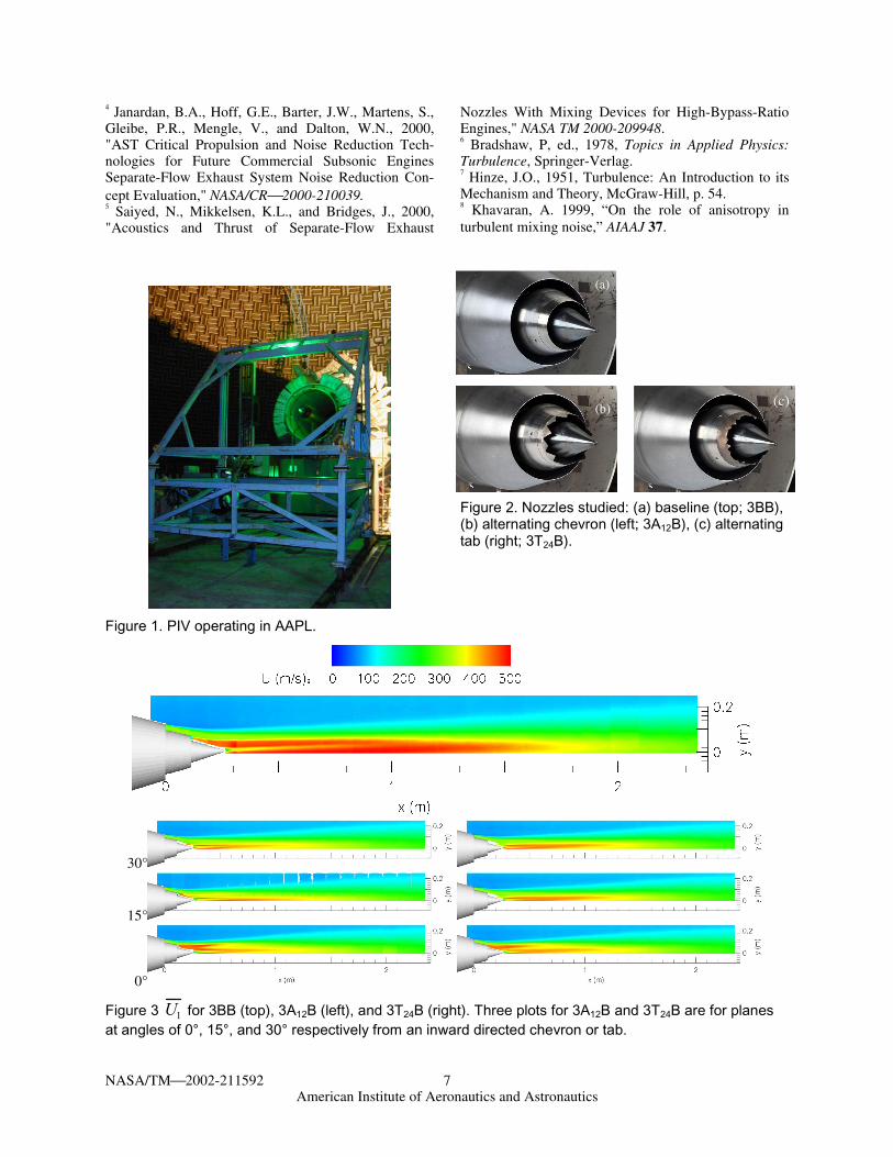
Many of the results will be presented as contour plots of the jet plume. In these plots the 3BB nozzle is shown on top, while the 3A12B is shown on the left and the 3T24B nozzle on the right. For these last two nozzles, are pre-sented in 3 radial planes clocked at (from the topmost figure) 30°, 15°, and 0° from the outward-bent chevron or tab. Since the flows all had 6-fold symmetry in their cross-section, the 30° sector represents a repeating pie segment of the flow for the entire cross-section. Previ-ous cross-sections taken with temperature and pressure rakes assured that the flow was satisfactorily symmetric.

Mean velocities

First, consider axial mean velocity, given in Figure 3 for the three nozzles. The axisymmetric flow field has an extended region, out to 2m, or 8 fan diameters, with velocities above 450m/s. In contrast, the two enhanced mixer nozzles produce flow fields where the mean ve-locity is below 400ms within 1.5m, or 6 fan diameters. While subtle differences exist between the two mixer nozzle flow fields, they are very similar, with both pro-ducing strong spread and a high speed ejection in the 0° plane. The increased mixing and subsequent reduction in high mean velocities is obvious.

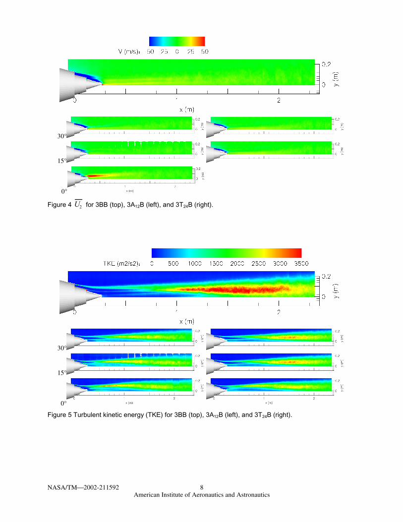
Looking at mean radial velocities in Figure 4, we notice the dramatic radially outward core velocities just down-stream of the plug in the 0° plane of the 3A12B and 3T24B flow fields. Again, the differences between the two mixers is small, both peaking around 75m/s, with the 3A12B nozzle having just slightly stronger radial outflow than the 3T24B. There is some compensating inward flow in the 30° plane where again the radial flow of the 3A12B nozzle is slightly stronger.

Turbulence

In separate flow nozzles three main mixing regions are traditionally identified: the inner shear layer between core and fan flows, the outer shear layer between the fan and ambient flows, and the jet mixing region, lo-cated roughly where an equivalent single-flow jet would have peak turbulence. The baseline nozzle flow has peak turbulent kinetic energy (TKE) between 1 and 2 m (4–8 fan diameters) downstream of the fan exit, e.g., the jet mixing region, as shown in Figure 5. The peak TKE is approximately 3500 m2/s2 but there is a large extent where the TKE is greater than 3000 m2/s2. In the 3A12B nozzle the TKE in the jet mixing region is greatly reduced—from 3500 m2/s2 down to 2500 m2/s2. Alternating chevrons create considerable turbulence at 0° azimuth (downstream of the outward chevron) around 0.6m, of 2.4 fan diameters downstream in the fan/core shear layer where the core flow pushes out-ward through the fan flow and produces a strong shear as it nearly contacts the ambient fluid. In fact, this is the

strongest region of turbulence in this jet, with TKE reaching over 3000 m2/s2. The 3T24B nozzle does not have quite as much reduction in the jet mixing region downstream, but also does not produce as much TKE in the region near 0.6m.

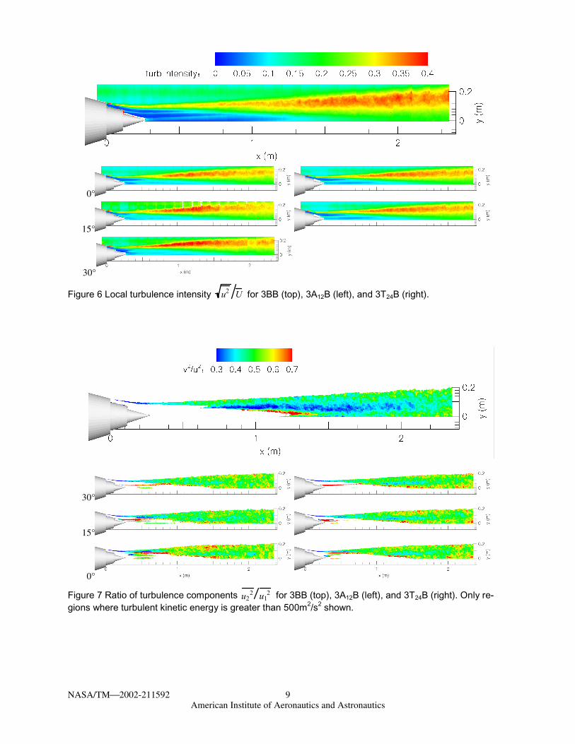
The logical question arising from Figure 5 is, “Have the chevrons actually modified the turbulence such that turbulence intensity is reduced?” Figure 6 shows that in

fact the local intensity Uu2 has been redistributed,

but that the peak local intensity in the jet mixing region is pretty much the same as it was in the baseline case. The main effect of the chevrons is to increase the turbu-lence intensity upstream of the jet mixing region. Not shown are the figures for turbulence intensity as nor-malized by the jet exit velocity. These fields look like those of Figure 5 and in the case of the 3BB nozzle peak around 14%.

The ratio of radial to axial turbulence 21

22 uu is of

interest in jet noise theory, and is shown in Figure 7. In these plots the turbulent kinetic energy has been used to highlight the regions where acoustic sources are strong (TKE > 500m2/s2). This ratio is different between the enhanced mixing nozzles and the baseline nozzle. The baseline nozzle has a ratio of 0.3–0.35 in the jet mixing region, while the enhanced mixing nozzles have a ratio of 0.45–0.55 in this region. Thus, besides reducing the turbulence in the jet mixing region of the jet plume, the mixing enhancement devices also make the turbulence more isotropic.

Integral Lengthscales

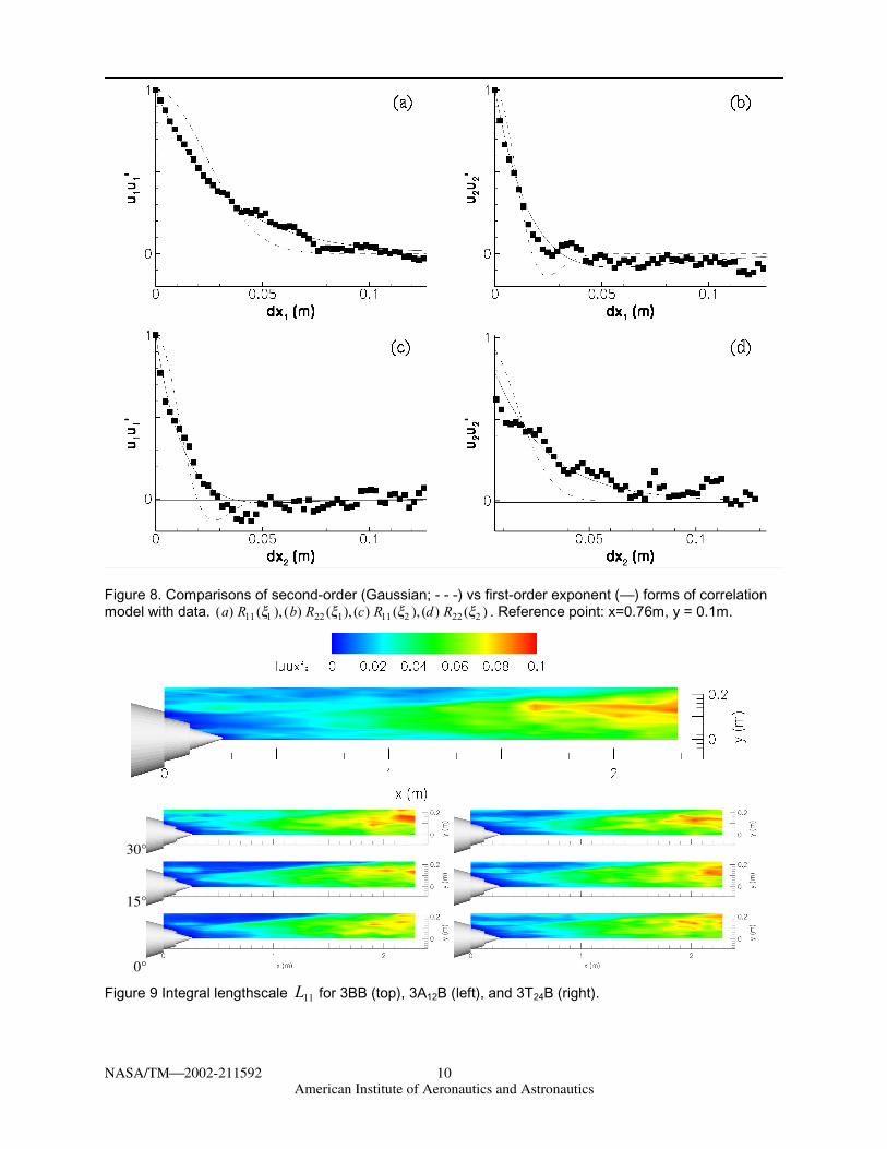
Two-point correlations were calculated from the veloc-ity maps, and integral lengthscales were computed from these correlations. In its most basic definition, the inte-gral lengthscale is determined by integrating the two-point correlation about its reference point, an approach that can be inaccurate both by assumption of homoge-neity and lack of enough displacement to reach conver-gence. The insensitivity of the lengthscale measurement to whether the two-point correlations were normalized by reference point variances or local variances indi-cated that the lengthscale measurement is not strongly affected by the lack of homogeneity in the radial direc-tion. To mitigate the latter error, two-point correlations were only computed about reference points in the axial center of the PIV velocity maps, and integrals were computed from fitted functions. Specifically, the corre-lations were fitted using the axisymmetric, single-power exponential forms given in equation (9) so that the integrals would not be truncated by the limited ex-tent of the displacement.

Obviously, when using the fitted curves to compute the integral lengthscales it is crucial that the appropriate-ness of the model be examined. To illustrate the fidelity with which the proposed model fit the two-point

NASA/TM2002-211592 6 American Institute of Aeronautics and Astronautics

correlation data, a representative set of curves is given in Figure 8. Two components of the correlation tensor Rii , are shown plotted on principle axes of the dis-placement vector ξk . Both data and curve fits using Gaussian (equation 7) and single-power exponential (equation 9) forms of the two-point correlation model are given. In all cases the single-power exponent model provides the best fit and is a reasonable approximation of the experimental data. Quantitatively, the variance of the fits were 0.01 or less (R2 > 0.99) for virtually the entire plume in all nozzles, with the radial correlations being especially well fit. Hence, the integral values calculated from the fitted curves will be shown here.

The axial lengthscale from axial velocity, L11 , is plot-ted for all models in Figure 9. Lengthscale values start around 0.005m in the inner and outer shear layers and reaching a value of almost 0.1m by the end of the measurement region 2.3m downstream. Because of the mesh spacing upon which velocities were measured, there is a lower bound on lengthscale of approximately 0.003m.

Within the experimental uncertainty obvious in the noise of the plots, there is very little difference between L11 for the 3BB and enhanced mixing nozzles, or be-tween the different planes of the enhanced mixing noz-zle plumes. So while the mixing enhancement devices do alter the turbulence intensity and ratio of turbulence intensities, they do not seem to change the lengthscale distribution appreciably.

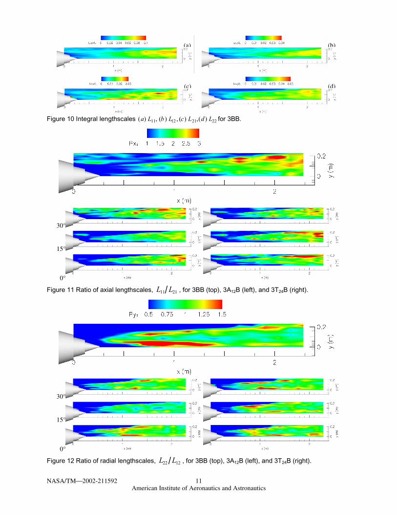
To compare the various lengthscales in a plume, L11, L12 , L21, L22 are plotted in Figure 10 for the 3BB nozzle. Not shown are the other lengthscales for the enhanced mixing nozzles, which are similar to that of 3BB. Carefully note the legend for the contour levels in the Figure. The main difference one observes between the plots within Figure 10 is the large integral lengthscales of the radial velocities near the jet axis, both in separations in x and in y. The cause for this is not known, but might be related to a suspected separa-tion from the end of the plug, the wake being well cor-related for a long distance downstream.

The ratio of lengthscales, e.g. L11 L21 and L22 L12 , is a value of interest in jet noise modeling. When the ra-tios of lengthscales are calculated from the experimen-tal results and plotted, as they are in Figure 11 and Figure 12, the fields are found not to be very uniform due to experimental uncertainty. This is especially true on the low-speed edge of the jet and the aforementioned anomalies near the centerline just downstream of the plug. In the estimate from the axial lengthscales, L11 L21 (Figure 11), the lengthscale ratio is roughly 2 throughout the jet mixing region. In the estimate from the radial lengthscales, L22 L12 (Figure 12), the ratio is

fairly uniform at a value of around 1. However, one cannot simply use these values as a global parameter in the prediction of jet noise due to the fact that the differ-ent nozzles have different distributions of TKE. For example, the 3A12B nozzle has significant turbulence around 0.6m where the lengthscale ratio L11 L21 is closer to 1 than to 2.

As pointed out above, in both isotropic and axisymmet-ric turbulence, the ratio L22 L12 should be exactly 2, a result clearly at variance with the present data, where the value is closer to 1. This discrepancy will need to be investigated in future work and perhaps a more compli-cated turbulence model developed to match these ob-servations.

Summary of Findings

Main findings:

• Mean velocity of the jet plume was lowered nearly equally by both the chevron and tab mixing en-hancement devices.

• Turbulent kinetic energy in the jet mixing region was lowered by both the chevron and tab mixing enhancement devices. Turbulence in the first two fan diameters was increased in the fan/core shear layer, especially in the radial plane including the outward chevron or tab. The chevron nozzle had the greatest increase in turbulence in the fan/core shear layer.

• Ratio of axial to radial components of turbulence was changed by the mixing enhancement devices, becoming more isotropic.

• Integral lengthscales in the jet plume are not sig-nificantly affected by the mixing enhancement de-vices, varying by roughly two orders of magnitude over the first 10 fan diameters of the flow. How-ever, the change in TKE produced by the chevrons means that peak turbulence regions had different lengthscales in the mixing enhancement nozzles.

• Ratios of integral lengthscales do not agree with isotropic or axisymmetric turbulence models, espe-cially for transverse separations.

References

1 Saiyed, N., ed., 2000, "Separate Flow Nozzle Test Status Meeting," NASA/CP2000-210524. 2 Long, M.J., 1992, “Experimental Investigation of an Ejector-Powered Free-Jet Facility,” NASA TM–105868. 3 Wernet, M.P., 1999, “Fuzzy Logic Enhanced Digital PIV Processing Software,” NASA/TM1999-209274.

NASA/TM2002-211592 7 American Institute of Aeronautics and Astronautics

4 Janardan, B.A., Hoff, G.E., Barter, J.W., Martens, S., Gleibe, P.R., Mengle, V., and Dalton, W.N., 2000, "AST Critical Propulsion and Noise Reduction Tech-nologies for Future Commercial Subsonic Engines Separate-Flow Exhaust System Noise Reduction Con-cept Evaluation," NASA/CR2000-210039. 5 Saiyed, N., Mikkelsen, K.L., and Bridges, J., 2000, "Acoustics and Thrust of Separate-Flow Exhaust

Nozzles With Mixing Devices for High-Bypass-Ratio Engines," NASA TM 2000-209948. 6 Bradshaw, P, ed., 1978, Topics in Applied Physics: Turbulence, Springer-Verlag. 7 Hinze, J.O., 1951, Turbulence: An Introduction to its Mechanism and Theory, McGraw-Hill, p. 54. 8 Khavaran, A. 1999, “On the role of anisotropy in turbulent mixing noise,” AIAAJ 37.

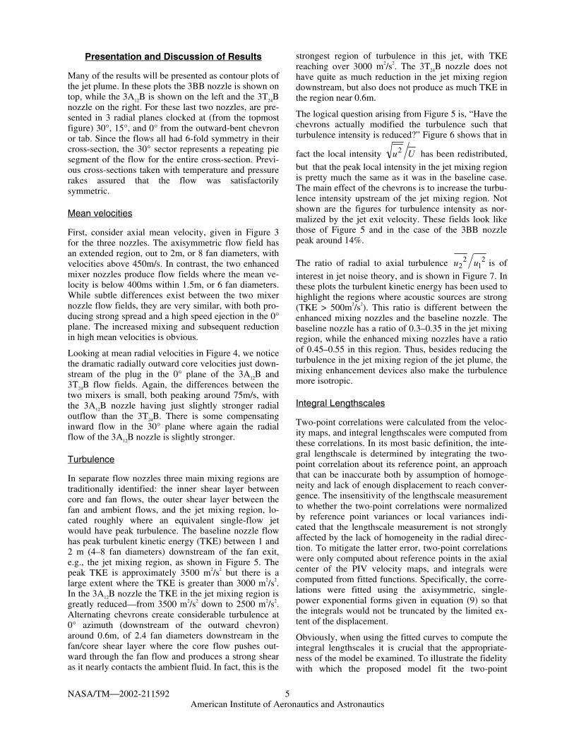
Figure 1. PIV operating in AAPL.

Figure 2. Nozzles studied: (a) baseline (top; 3BB), (b) alternating chevron (left; 3A12B), (c) alternating tab (right; 3T24B).

30°

15°

0°

Figure 3 U1 for 3BB (top), 3A12B (left), and 3T24B (right). Three plots for 3A12B and 3T24B are for planes at angles of 0°, 15°, and 30° respectively from an inward directed chevron or tab.

(a)

(b) (c)

NASA/TM2002-211592 8 American Institute of Aeronautics and Astronautics

30°

15°

0°

Figure 4 U2 for 3BB (top), 3A12B (left), and 3T24B (right).

30°

15°

0°

Figure 5 Turbulent kinetic energy (TKE) for 3BB (top), 3A12B (left), and 3T24B (right).

NASA/TM2002-211592 9 American Institute of Aeronautics and Astronautics

0°

15°

30°

Figure 6 Local turbulence intensity u2 U for 3BB (top), 3A12B (left), and 3T24B (right).

30°

15°

0°

Figure 7 Ratio of turbulence components u22 u1

2 for 3BB (top), 3A12B (left), and 3T24B (right). Only re-gions where turbulent kinetic energy is greater than 500m2/s2 shown.

NASA/TM2002-211592 10 American Institute of Aeronautics and Astronautics

Figure 8. Comparisons of second-order (Gaussian; - - -) vs first-order exponent (—) forms of correlation model with data. (a) R11 (ξ1 ), (b) R22 (ξ1), (c) R11 (ξ2 ), (d ) R22 (ξ2 ) . Reference point: x=0.76m, y = 0.1m.

30°

15°

0°

Figure 9 Integral lengthscale L11 for 3BB (top), 3A12B (left), and 3T24B (right).

NASA/TM2002-211592 11 American Institute of Aeronautics and Astronautics

Figure 10 Integral lengthscales (a) L11, (b ) L12 , (c) L21,(d ) L22 for 3BB.

30°

15°

0°

Figure 11 Ratio of axial lengthscales, L11 L21 , for 3BB (top), 3A12B (left), and 3T24B (right).

30°

15°

0°

Figure 12 Ratio of radial lengthscales, L22 L12 , for 3BB (top), 3A12B (left), and 3T24B (right).

(a) (b)

(c) (d)

This publication is available from the NASA Center for AeroSpace Information, 301–621–0390.

REPORT DOCUMENTATION PAGE

2. REPORT DATE

19. SECURITY CLASSIFICATION OF ABSTRACT

18. SECURITY CLASSIFICATION OF THIS PAGE

Public reporting burden for this collection of information is estimated to average 1 hour per response, including the time for reviewing instructions, searching existing data sources,gathering and maintaining the data needed, and completing and reviewing the collection of information. Send comments regarding this burden estimate or any other aspect of thiscollection of information, including suggestions for reducing this burden, to Washington Headquarters Services, Directorate for Information Operations and Reports, 1215 JeffersonDavis Highway, Suite 1204, Arlington, VA 22202-4302, and to the Office of Management and Budget, Paperwork Reduction Project (0704-0188), Washington, DC 20503.

NSN 7540-01-280-5500 Standard Form 298 (Rev. 2-89)Prescribed by ANSI Std. Z39-18298-102

Form Approved

OMB No. 0704-0188

12b. DISTRIBUTION CODE

8. PERFORMING ORGANIZATION REPORT NUMBER

5. FUNDING NUMBERS

3. REPORT TYPE AND DATES COVERED

4. TITLE AND SUBTITLE

6. AUTHOR(S)

7. PERFORMING ORGANIZATION NAME(S) AND ADDRESS(ES)

11. SUPPLEMENTARY NOTES

12a. DISTRIBUTION/AVAILABILITY STATEMENT

13. ABSTRACT (Maximum 200 words)

14. SUBJECT TERMS

17. SECURITY CLASSIFICATION OF REPORT

16. PRICE CODE

15. NUMBER OF PAGES

20. LIMITATION OF ABSTRACT

Unclassified Unclassified

Technical Memorandum

Unclassified

National Aeronautics and Space AdministrationJohn H. Glenn Research Center at Lewis FieldCleveland, Ohio 44135–3191

1. AGENCY USE ONLY (Leave blank)

10. SPONSORING/MONITORING AGENCY REPORT NUMBER

9. SPONSORING/MONITORING AGENCY NAME(S) AND ADDRESS(ES)

National Aeronautics and Space AdministrationWashington, DC 20546–0001

Available electronically at http://gltrs.grc.nasa.gov/GLTRS

June 2002

NASA TM—2002-211592AIAA–2002–2484

E–13376

WU–781–30–12–00

17

Turbulence Measurements of Separate Flow Nozzles With MixingEnhancement Features

James Bridges and Mark P. Wernet

Noise prediction; Aircraft; Turbulence models; Shear layers; Jet mixing; Flow;Noise reduction; Jet aircraft noise; Turbulence

Unclassified -UnlimitedSubject Categories: 07 and 34 Distribution: Nonstandard

Prepared for the Eighth Aeroacoustics Conference cosponsored by the American Institute of Aeronautics and Astronauticsand the Confederation of European Aerospace Societies, Breckenridge, Colorado, June 17–19, 2002. Responsible person,James Bridges, organization code 5940, 216–433–2693.

Comparison of turbulence data taken in three separate flow nozzles, two with mixing enhancement features on their corenozzle, shows how the mixing enhancement features modify turbulence to reduce jet noise. The three nozzles measuredwere the baseline axisymmetric nozzle 3BB, the alternating chevron nozzle, 3A12B, with 6-fold symmetry, and the flippertab nozzle 3T24B also with 6-fold symmetry. The data presented show the differences in turbulence characteristicsproduced by the geometric differences in the nozzles, with emphasis on those characteristics of interest in jet noise.Among the significant findings: the enhanced mixing devices reduce turbulence in the jet mixing region while increasingit in the fan/core shear layer, the ratios of turbulence components are significantly altered by the mixing devices, and theintegral lengthscales do not conform to any turbulence model yet proposed. These findings should provide guidance formodeling the statistical properties of turbulence to improve jet noise prediction.