Turbulence modeling of deep dynamic stall at relatively low Reynolds number

Contents lists available at SciVerse ScienceDirect

Journal of Fluids and Structures

Journal of Fluids and Structures 33 (2012) 191–209

0889-97

http://d

n Corr

E-m

journal homepage: www.elsevier.com/locate/jfs

Turbulence modeling of deep dynamic stall at relatively lowReynolds number

Shengyi Wang a,b, Derek B. Ingham a, Lin Ma a,n, Mohamed Pourkashanian a, Zhi Tao b

a Centre for CFD, Energy Technology and Innovation Initiative, Faculty of Engineering, The University of Leeds, Leeds LS2 9JT, UKb National Key Laboratory of Science and Technology on Aero-Engine Aero-thermodynamics, School of Jet Propulsion, Beijing University of Aeronautics and

Astronautics, Beijing 100191, China

a r t i c l e i n f o

Article history:

Received 12 May 2011

Accepted 30 April 2012Available online 18 June 2012

Keywords:

DDES

Dynamic stall

Low Reynolds number

URANS

Wind turbine

46/$ - see front matter & 2012 Elsevier Ltd. A

x.doi.org/10.1016/j.jfluidstructs.2012.04.011

esponding author. Tel.: þ44 113 3438954; f

ail addresses: [email protected], gmwsy@163

a b s t r a c t

This paper investigates numerically the unsteady separated turbulent flows around an

oscillating airfoil pitching in a sinusoidal pattern that induces deep dynamic stalls. The

flow is in the regime of relatively low Reynolds number of the order of 105 based on the

chord length of the airfoil. Both the URANS and the more advanced DES approaches are

employed. The URANS is coupled with two advanced turbulence models, namely the

RNG k�e model and the Transition SST model (g�Rey model) and the DES is coupled

with the SST k�o model. A comparison with experimental data shows that the SST

k�o based DES approach is superior to the URANS approach and presents generally

good agreement with the experimental data, although the prediction of experimentally

observed peek stall angle of attack may not be warranted. The details of the complex

flow development of the dynamic stall and the boundary layer transition have been

discussed.

& 2012 Elsevier Ltd. All rights reserved.

1. Introduction

Dynamic stall is a phenomenon involving a series of fluid flow separations and reattachments that occur on an airfoil, orany other lifting surface, when it is subjected to a rapid unsteady motion such as pitching, flapping, and plunging orvertical translating movements in the fluid flow with its maximum angle of attack being above its normal static stall angle(Leishman, 2006). Dynamic stall significantly affects the aerodynamic performance of a large variety of fluid machinery(Ericsson and Reding, 1988), such as helicopters, highly maneuverable fighter jets, gas turbines, and modern wind turbines(Galvanetto et al., 2008). A typical deep dynamic stall process can be categorized into four key stages, i.e. an attached flowat low angles of attack, the development of the leading edge vortex (LEV), the shedding of the LEV from the suction surfacecausing the full stall of the blade, and the reattachment of the flow to the suction surface (Wernert et al., 1996). Althoughthe basic image of the dynamic stall has been generally clarified, the physics of this strongly non-linear unsteady flowphenomenon has not yet been completely understood, in particular under a relatively low Reynolds number such as of theorder of 105 where complex boundary layer flow transition occurs. More efforts are required to advance the knowledge tothe level on which the phenomenon can be accurately predicted and precisely controlled.

Dynamic stall has important impact on the aerodynamic performance of wind energy conversion devices in terms ofboth horizontal axis wind turbines (HAWT) and vertical axis wind turbines (VAWT). For HAWTs, dynamic stall can occur

ll rights reserved.

ax: þ44 113 2467310.

.com (L. Ma).

www.elsevier.com/locate/jfs

www.elsevier.com/locate/jfs

dx.doi.org/10.1016/j.jfluidstructs.2012.04.011



mailto:[email protected]

mailto:[email protected]


S. Wang et al. / Journal of Fluids and Structures 33 (2012) 191–209192

under a wide range of flow conditions, including free stream turbulence, tower shadow, and yawed flow. However, theaerodynamics of the HAWTs under the conditions such as yawing is very similar to what occurs when the blade performs aharmonic pitching, as investigated in this paper, in terms of the formation of the leading edge vortex, vortex shedding, etc.,due to the constant changing in the angle of attack (AOA) perceived by the turbine blades (Hansen and Butterfield, 1993).For VAWTs, in particular the Darrieus type, or lift-driven type turbine, the flow perceived by the turbine blade also variescyclically in both direction and magnitude leading to almost constant occurrences of the dynamic stall in the operation ofthese types of wind turbines (Fraunie et al., 1986). In addition to the aerodynamic performance, the dynamic stall is also asubstantial source of the structural vibration pertinent to the fatigue life of the turbine (McLaren et al., in press). Thisphenomena is also strongly analogous to that observed on a harmonic pitching blade in the fluid stream (Wang et al.,2010a). However, the variation in the magnitude of the relative incoming air velocity received by the VAWT blades atdifferent positions of their flying path adds to the complexity of the problem.

Most of the previous researches on dynamic stall have been devoted to flows at relatively high Reynolds numbers (ReZ106)or at a moderate to high Mach number (MaZ0.3) that often fall into the compressible flow regime typical for turbomachinery,aircraft or helicopter rotors operating at high speed. Also, some are in the context of very low Re(102–103) which concernslaminar flows(Amiralaei et al., 2010). Although the range of Re for the modern HAWT can be as high as 2�106 (Hansen andButterfield, 1993), or even higher for some MW scale turbines, for small-to-medium sized VAWTs, such as the recently risingH-type Darrieus turbines, it is common to operate with Re of the order 105 or even lower (Sheldahl et al., 1980). Flows withsuch relatively low Reynolds number are highly non-linear (Poirel et al., 2011) and deep stall are often associated with leadingedge separation and in particular, boundary layer transitions from laminar to turbulent flows, which are very sensitive to localadverse pressure gradients as well as the advection scheme and turbulence model employed. This makes accurate predictionsof the flow separation and the onset of the dynamic stall much more difficult. In general, dynamic stall at this relatively lowReynolds number, which is relevant to low speed wind turbine conditions, has been less well investigated.

In terms of numerical simulation of the dynamic stall process, very limited research literature is available for therelatively low Reynolds number regime. Martinat et al. (2008) did attempt to evaluate the ability of the unsteadyReynolds-Averaged Navier–Stokes (URANS) approach and the delayed detached eddy simulation (DDES) to model thedynamic stall when the blade is undertaking an oscillating movement with Re ranging from 105 to 106. The DDES modelpredicted that the lift and drag coefficients are in good general agreement with the experimental data for the high Re caseinvestigated. It is noted that the DDES predictions do not show significant improvements over the URANS predictions. Inparticular, both the URANS and DDES approaches missed the peak values of the lift and drag coefficients for the casestudied. The turbulence models employed in their URANS study include the Spalart-Allmaras model, k�e Chien model, SSTk�o model, and the so-called Organized Eddy Simulation (OES) for modeling the non-equilibrium turbulence effects. Thesimulations were performed in both 2-D and 3-D and the authors concluded that the flow is practically two-dimensionalduring the up-stroke and the separated flow during the down-stroke shows strong 3-D effects. Although a qualitative flowtopology is generally obtained, none of the models present a satisfactory agreement with the corresponding experimentaldata in their study, in particular at the down-stroke phase and there is a significant overshoot in the lift coefficient peak.Since the location of the onset of transition has a significant impact on the overall dynamic stall process for relatively lowReynolds number flows, this has to be considered in order to improve the accuracy of the simulations.

In addition, Spentzos et al., (2005) have performed a numerical investigation into the dynamic stall over an oscillatingblade with an even lower Re of 104–105, again using the URANS method but coupled with the baseline k�o model. Thevelocity profiles and pressure distributions obtained were compared with the corresponding experimental data with areasonably good agreement being obtained. However, no validation on the predicted aerodynamic forces on the oscillatingblade was reported. Wang et al. (2010a) and Wang et al. (2010b) performed a further series of numerical investigations toassess the ability of various turbulence models to simulate the dynamic stall at relatively low Reynolds numbers where theStandard k�o model, SST k�o model and the n2

� f model are employed. The SST k�o model and the n2� f model can

predict the lift and drag for a large portion of the up-stroke phase well, except at high AOAs and both models fail toreproduce flow reattachments accurately over the down-stroke phase.

The aim of the present paper is to further investigate the available numerical techniques in order to improve the CFDpredictions of deep dynamic stall with a reduced frequency and Reynolds number that is close to the conditions thattypically occur in small-to-medium scale wind turbines. So far, although some of the turbulence models can reasonablypredict the attached flow in the up-stroke phase of an oscillating blade, none of the models investigated show goodpredictions of the peak force coefficients or the corresponding angle of attack, the down-stroke phase and the flowreattachments. The work is based on the authors’ previous work (Wang et al., 2010a; Wang et al., 2010b) and is inparticular to assess the more advanced Transition SST (g�Rey model) turbulence model (ANSYS, 2009) with URANS forimproving predictions of transition onset which is closely related to the peak lift that the aerofoil can achieve. Also,investigations have been performed on the delayed detached eddy simulation (DDES) technique for its ability to reproducethe complex flow conditions in the down-stroke phase which is crucial for the subsequent flow reattachments. A relativelylow mean angle of attack that can be found in the literature which is more pertinent to wind turbine conditions has beenemployed. The results obtained have been compared with experimental data and those obtained with the relatively simpleRNG k�e model in terms of their capability in capturing the dynamic stall flow characteristics and the aerodynamic forces.Simulations have been performed both in 2-D and 3-D. This paper contributes to an improved understanding of CFDpredictions of unsteady aerodynamic flows.

S. Wang et al. / Journal of Fluids and Structures 33 (2012) 191–209 193

2. Numerical models and case studied

Various stages of the dynamic stall process can be well represented by the fluid flows over an oscillating airfoil pitchingin a sinusoidal pattern a¼a0þal sin(ot). Extensive investigations on a variety of oscillating patterns of airfoils have beenconducted experimentally in wind tunnels (Carr, 1988; McCroskey et al., 1976; McCroskey et al., 1982). However,relatively low Reynolds number investigations with available data and flow configurations pertinent to wind turbineapplications are very limited. In the present paper, the experimental work of Lee and Gerontakos (2004) is numericallystudied. The primary reason for selecting this experimental work as a validation case is that the Reynolds number of thefree stream investigated falls in the range that is relevant to the operations of small-to-medium scale wind turbines. Theexperimental setup, such as the wind speed and the oscillating rate o, is also comparable to the situation of a typical smallscale Darrieus VAWT. On the other hand, much care has been taken in the experiments to eliminate the 3-D flow effects onthe measurement plane. Therefore, the data obtained can be employed with confidence for the purpose of validating 2-Dnumerical simulations. However, turbulence is three-dimensional in nature and in particular when it involves severe flowseparations, such as under stall conditions in the down-stroke motion of an oscillating aerofoil. In addition to the detailed2-D simulations using URANS models, 3-D calculations have been performed and analyzed with both URANS and DDESturbulence simulation techniques, although the 3-D effects are more of a secondary phenomenon, in particular underattached flow conditions for the case investigated. It does show its effect in the vicinity of stall and the down-stroke phase.However, it should be noted that even with the current available HPC computer powers, performing 3-D DES typesimulations of the dynamic stall process for engineering applications, which require substantially fine mesh and temporalsteps, is very computationally demanding.

2.1. Case studied

Corresponding to the work of Lee and Gerontakos (2004), the airfoil employed in the numerical calculations is a NACA0012 airfoil with a chord length of c¼0.15 m and a span of h¼0.375 m. The airfoil executes a sinusoidal pitching with amean angle of attack a of 101, i.e. a¼101

þ151 sin(18.67t), and a reduced frequency of k¼oc/2UN¼0.10, around an axislocated at a quarter of its chord (0.25c) from the leading edge. The mean free stream velocity UN is 14 m/s whichcorresponds to a Reynolds number of Rec¼1.35�105 based on the chord length of the airfoil. The turbulence intensity ofthe free stream is 0.08%. Two end plates were fitted in the experiments to minimize the flow leakage from the blade tip(blade tip effects) and to eliminate as much as possible any substantial 3-D effects of the flow at the measurement locationat the mid-section of the blade. By checking the blade wake flow, the flow non-uniformity along the spanwise directionwas found to be negligible in the experimental investigations. A comprehensive description of the experimental setup isdetailed in Lee and Gerontakos (2004).

2.2. Numerical techniques

In this study, the simulations based on the URANS method are first performed. The reasons for this are as follows:

(i)
Numerical studies using URANS incorporating three turbulence models, namely the standard k�o model, SST k�omodel and the n2
� f model, have been performed in the authors’ previous work (Wang et al., 2010a, 2010b) and it wasfound that the URANS approach can qualitatively capture some of the major flow features involved in the dynamicstall, such as the development of the leading edge vortex (LEV) and the hysteresis loop of the dynamic loading actingon the airfoil. However, all the tested turbulence models fail to accurately reproduce the performance of the airfoilclose to the stall and during the post-stall phases. Thus it is necessary to further assess other advanced and recentlyavailable turbulence models, such as the Transition SST turbulence model, emphasizing on the transition onsetpredictions.

(ii)
URANS is still the work horse of CFD for industrial flow applications where it is intuitive to use simple turbulencemodels, such as the RNG k�e model and it is numerically less expensive than the more complex eddy resolvedmethods, such as the detached eddy simulation (DES) and the large eddy simulation (LES). However the accuracy ofthe numerical predictions employing simple turbulence models needs to be quantified.
(iii)
The turbulence field obtained from the URANS results can be used as a guide in the design of the computational gridfor the subsequently performed DDES.
The incompressible Navier–Stokes equations are solved since the March number of the flow investigated in this paper islow. The employed solver is a pressure-based segregated solver that calculates the continuity, momentum, and turbulenceequations in double precision. In terms of pressure–velocity coupling, the commonly used SIMPLE algorithm is employed.The temporal term has been discretized with a first-order implicit scheme due to the limitation of the software. However,care has been taken to make sure that the time-step employed is small enough to obtain accurate numerical solutions.The convective terms in the URANS equations are discretized with a second-order upwind scheme and the diffusive termsare approximated by second-order central differencing. For DDES, the Bounded Central Differencing scheme is adopted.


In order to accelerate the rate of solution convergence, the algebraic multi-grid method (AMG) is applied in which theV-cycle is used for the pressure equation in the pressure-based segregated algorithm and the flexible cycle is used for allthe other equations. A multi-grid cycle can be defined as a recursive procedure that is applied at each grid level as it movesthrough the grid hierarchy. The detailed information of the solver setup can be found in ANSYS (2009).

2.2.1. Grid design

The quality of the computational grids is of crucial importance for the accuracy of the CFD solutions and therefore thephilosophy of the grid generation is discussed below.

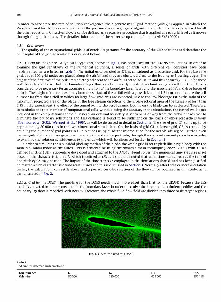
2.2.1.1. Grid for the URANS. A typical C-type grid, shown in Fig. 1, has been used for the URANS simulations. In order toexamine the grid sensitivity of the numerical solutions, a series of grids with different cell densities have beenimplemented, as are listed in Table 1. The initial grid, denoted as G1, is considered as a baseline grid. For this baselinegrid, about 300 grid nodes are placed along the airfoil and they are clustered close to the leading and trailing edges. Theheight of the first row of the cells immediately adjacent to the airfoil is set to be 10�5c and this ensures yþr1.0 for thesewall boundary cells so that the boundary layer flow can be properly resolved without using a wall function. This isconsidered to be necessary for an accurate simulation of the boundary layer flows and the associated lift and drag forces ofairfoils. The height of the cells expands from the surface of the airfoil with a growth factor of 1.2 in order to reduce the cellnumber far from the airfoil in which no large flow gradients are expected. Due to the low blockage ratio (the ratio of themaximum projected area of the blade in the free stream direction to the cross-sectional area of the tunnel) of less than2.5% in the experiment, the effect of the tunnel wall to the aerodynamic loading on the blade can be neglected. Therefore,to minimize the total number of computational cells, without losing the accuracy in the simulations, the tunnel wall is notincluded in the computational domain. Instead, an external boundary is set to be 20c away from the airfoil at each side toeliminate the boundary reflections and this distance is found to be sufficient on the basis of other researchers work(Spentzos et al., 2005; Wernert et al., 1996), as will be discussed in detail in Section 3. The size of grid G1 sums up to beapproximately 80 000 cells in the two-dimensional simulations. On the basis of grid G1, a denser grid, G2, is created, bydoubling the number of grid points in all directions using quadratic interpolation for the near-blade region. Further, evendenser grids, G3 and G4, are generated based on G2 and G3, respectively, through the same refinement procedure in orderto examine the solution sensitiveness to the grids which will be discussed further in Section 3.

In order to simulate the sinusoidal pitching motion of the blade, the whole grid is set to pitch like a rigid body with thesame sinusoidal mode as the airfoil. This is achieved by using the dynamic mesh technique (ANSYS, 2009) with a userdefined function (UDF) subroutine developed and attached to the ANSYS Fluent solver. The numerical time step size is setbased on the characteristic time Tc which is defined as c/UN. It should be noted that other time scales, such as the time ofone pitch cycle, may be used. The impact of the time step size employed in the simulations should, and has been justifiedno matter which characteristic time scale is used and this is discussed in Section 3. Normally after three or more oscillationcycles, the calculations can settle down and a perfect periodic solution of the flow can be obtained in this study, as isdemonstrated in Fig. 2.

2.2.1.2. Grid for the DDES. The gridding for the DDES needs much more effort than that for the URANS because the LESmode is activated in the regions outside the boundary layer in order to resolve the larger scale turbulence eddies and theboundary lay flow is modeled with RANRS. Therefore, the whole fluid flow field are divided into three basic target regions

Fig. 1. C-type grid used for URANS.

Table 1Grid size for different grids employed.

Grid number G1 G2 G3 DESGrid size 80 000 180 000 605 000 185 118

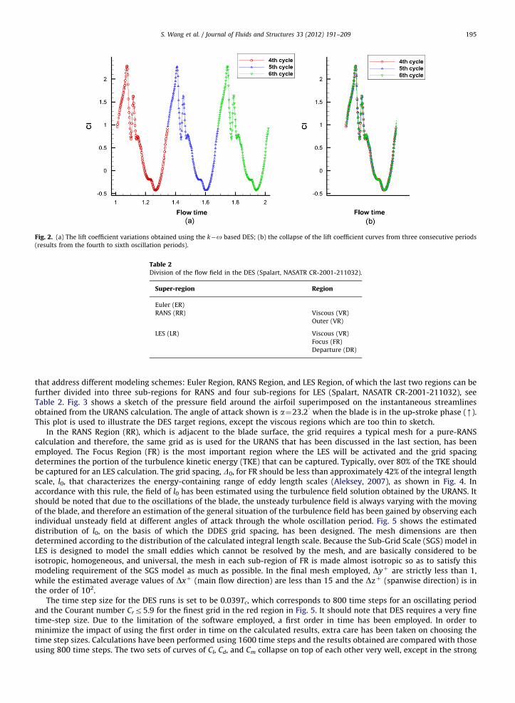
Fig. 2. (a) The lift coefficient variations obtained using the k�o based DES; (b) the collapse of the lift coefficient curves from three consecutive periods

(results from the fourth to sixth oscillation periods).

Table 2Division of the flow field in the DES (Spalart, NASATR CR-2001-211032).

Super-region Region

Euler (ER)

RANS (RR) Viscous (VR)

Outer (VR)

LES (LR) Viscous (VR)

Focus (FR)

Departure (DR)


that address different modeling schemes: Euler Region, RANS Region, and LES Region, of which the last two regions can befurther divided into three sub-regions for RANS and four sub-regions for LES (Spalart, NASATR CR-2001-211032), seeTable 2. Fig. 3 shows a sketch of the pressure field around the airfoil superimposed on the instantaneous streamlinesobtained from the URANS calculation. The angle of attack shown is a¼23.21 when the blade is in the up-stroke phase (m).This plot is used to illustrate the DES target regions, except the viscous regions which are too thin to sketch.

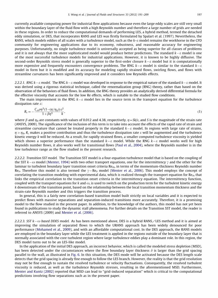
In the RANS Region (RR), which is adjacent to the blade surface, the grid requires a typical mesh for a pure-RANScalculation and therefore, the same grid as is used for the URANS that has been discussed in the last section, has beenemployed. The Focus Region (FR) is the most important region where the LES will be activated and the grid spacingdetermines the portion of the turbulence kinetic energy (TKE) that can be captured. Typically, over 80% of the TKE shouldbe captured for an LES calculation. The grid spacing, D0, for FR should be less than approximately 42% of the integral lengthscale, l0, that characterizes the energy-containing range of eddy length scales (Aleksey, 2007), as shown in Fig. 4. Inaccordance with this rule, the field of l0 has been estimated using the turbulence field solution obtained by the URANS. Itshould be noted that due to the oscillations of the blade, the unsteady turbulence field is always varying with the movingof the blade, and therefore an estimation of the general situation of the turbulence field has been gained by observing eachindividual unsteady field at different angles of attack through the whole oscillation period. Fig. 5 shows the estimateddistribution of l0, on the basis of which the DDES grid spacing, has been designed. The mesh dimensions are thendetermined according to the distribution of the calculated integral length scale. Because the Sub-Grid Scale (SGS) model inLES is designed to model the small eddies which cannot be resolved by the mesh, and are basically considered to beisotropic, homogeneous, and universal, the mesh in each sub-region of FR is made almost isotropic so as to satisfy thismodeling requirement of the SGS model as much as possible. In the final mesh employed, Dyþ are strictly less than 1,while the estimated average values of Dxþ (main flow direction) are less than 15 and the Dzþ (spanwise direction) is inthe order of 102.

The time step size for the DES runs is set to be 0.039Tc, which corresponds to 800 time steps for an oscillating periodand the Courant number Crr5.9 for the finest grid in the red region in Fig. 5. It should note that DES requires a very finetime-step size. Due to the limitation of the software employed, a first order in time has been employed. In order tominimize the impact of using the first order in time on the calculated results, extra care has been taken on choosing thetime step sizes. Calculations have been performed using 1600 time steps and the results obtained are compared with thoseusing 800 time steps. The two sets of curves of Cl, Cd, and Cm collapse on top of each other very well, except in the strong

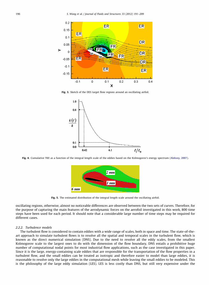
Fig. 3. Sketch of the DES target flow regions around an oscillating airfoil.

Fig. 4. Cumulative TKE as a function of the integral length scale of the eddies based on the Kolmogorov’s energy spectrum (Aleksey, 2007).

Fig. 5. The estimated distribution of the integral length scale around the oscillating airfoil.


oscillating regions, otherwise, almost no noticeable differences are observed between the two sets of curves. Therefore, forthe purpose of capturing the main features of the aerodynamic forces on the aerofoil investigated in this work, 800 timesteps have been used for each period. It should note that a considerable large number of time steps may be required fordifferent cases.

2.2.2. Turbulence models

The turbulent flow is considered to contain eddies with a wide range of scales, both in space and time. The state-of-the-art approach to simulate turbulent flows is to resolve all the spatial and temporal scales in the turbulent flow, which isknown as the direct numerical simulation (DNS). Due to the need to resolve all the eddy scales, from the smallestKolmogorov scale to the largest ones to do with the dimension of the flow boundary, DNS entails a prohibitive hugenumber of computational nodal points for most industrial flow applications, such as the case investigated in this paper.Since it is the large, energy-containing scale eddies that are responsible for the transportation of the flow properties in aturbulent flow, and the small eddies can be treated as isotropic and therefore easier to model than large eddies, it isreasonable to resolve only the large eddies in the computational mesh while leaving the small eddies to be modeled. Thisis the philosophy of the large eddy simulation (LES). LES is less costly than DNS, but still very expensive under the


currently available computing power for industrial flow applications because even the large eddy scales are still very smallwithin the boundary layer of the fluid flow with a high Reynolds number and therefore a large number of grids are neededin these regions. In order to reduce the computational demands of performing LES, a hybrid method, termed the detachededdy simulation, or DES, that incorporates RANS and LES was firstly formulated by Spalart et al. (1997). Nevertheless, theRANS, which models eddies of all scales with a turbulence model, such as the k–e model remains the workhorse in the CFDcommunity for engineering applications due to its economy, robustness, and reasonable accuracy for engineeringpurposes. Unfortunately, no single turbulence model is universally accepted as being superior for all classes of problemsand it is not always that the more sophisticated model would produce better predictions. The standard k�e model is oneof the most successful turbulence models for industrial applications. However, it is known to be highly diffusive. Thesecond-order Reynolds stress model is generally superior to the first-order closure k�e model but it is computationallymore expensive and frequently encounters convergence problems. The RNG k�e model is similar to the standard k�emodel in form but it is modified and its accuracy for modeling rapidly strained flows, swirling flows, and flows withstreamline curvatures has been significantly improved and it considers low Reynolds effects.

2.2.2.1. RNG k�e model. The RNG k�e model was developed in response to the empirical nature of the standard k�e model. Itwas derived using a rigorous statistical technique, called the renormalization group (RNG) theory, rather than based on theobservation of the behaviors of fluid flows. In addition, the RNG theory provides an analytically derived differential formula forthe effective viscosity that accounts for the low Re effects, which is suitable to the studied flow conditions.

The main improvement in the RNG k�e model lies in the source term in the transport equation for the turbulencedissipation rate e:

Re ¼�CmrZ3ð1�ðZ=Z0ÞÞ

1þbZ3

e2

k, ð1Þ

where b and Z0 are constants with values of 0.012 and 4.38, respectively. Z¼Sk/e, and S is the magnitude of the strain rate(ANSYS, 2009). The significance of the inclusion of this term is to take into account the effects of the rapid rate of strain andstreamline curvature that cannot be treated properly in the standard k�e model. In regions with large rate of strains,Z4Z0, Re makes a positive contribution and thus the turbulence dissipation rate e will be augmented and the turbulencekinetic energy k will be reduced. As a result, for rapidly strained flows, a smaller computed turbulence viscosity is yieldedwhich shows a superior performance than the standard k�e model. While the RNG k�e model works well for highReynolds number flows, it also works well for transitional flows (Paul et al., 2004), where the Reynolds number is in thelow turbulence range as the flow studied in the present research.

2.2.2.2. Transition SST model. The Transition SST model is a four-equation turbulence model that is based on the coupling ofthe SST k�o model (Menter, 1994) with two other transport equations, one for the intermittency g and the other for thelaminar to turbulent boundary layer transition onset criteria Reyt, in terms of the momentum-thickness Reynolds numberRey. Therefore this model is also termed the g�Rey model (Menter et al., 2006). This model employs the concept ofcorrelating the transition modeling with experimental data, which is realized through the transport equation for Reyt thatlinks the empirical correlation to the transition onset criteria in the intermittency equation. The intermittency function,coupled with the transport equations for k and o, is used to switch on the production term for the turbulent kinetic energyk downstream of the transition point, based on the relationship between the local transition momentum thickness and thestrain-rate Reynolds number and this triggers the transition process.

In general, this is a fairly new correlation-based transition model built strictly on local variables and it is expected topredict flows with massive separations and separation-induced transitions more accurately. Therefore, it is a promisingmodel to the flow studied in the present paper. In addition, to the knowledge of the authors, this model has not yet beenfound in publications to study the dynamic stall phenomena. For further details on the Transition SST model, the reader isreferred to ANSYS (2009) and Menter et al. (2006).

2.2.2.3. SST k�o based DDES model. As has been mentioned above, DES is a hybrid RANSXLES method and it is aimed atimproving the simulation of separated flows to which the URANS approach has been widely denounced for poorperformance (Mohamed et al., 2009), and with an affordable computational cost. In the DES approach, the RANS modelsare employed in the boundary layer while the LES treatment is applied in the regions outside of the boundary layer that isnormally associated with the core turbulent region where large turbulence eddies play a dominant role. In this region, theDES model turns out to be an LES-like model.

In the application of the initial DES approach, an incorrect behavior, which is called the modeled stress depletion (MSD),has been detected under the circumstances where the flow boundary layer thickness d is larger than the grid spacingparallel to the wall, as illustrated in Fig. 6. In this situation, the DES mode will be activated because the DES length scaledetects that the grid spacing is already fine enough to follow the LES branch. However, the reality is that the grid resolutionmay not be fine enough to sustain the resolved turbulence or velocity fluctuations. Consequently, the resolved turbulentviscosity is reduced, as well as the turbulence Reynolds stresses, resulting in the aforementioned MSD. Furthermore,Menter and Kuntz (2002) reported that MSD can lead to ‘‘grid-induced separation’’ which is critical to the computationalpredictions involving flow separations such as in the present paper.

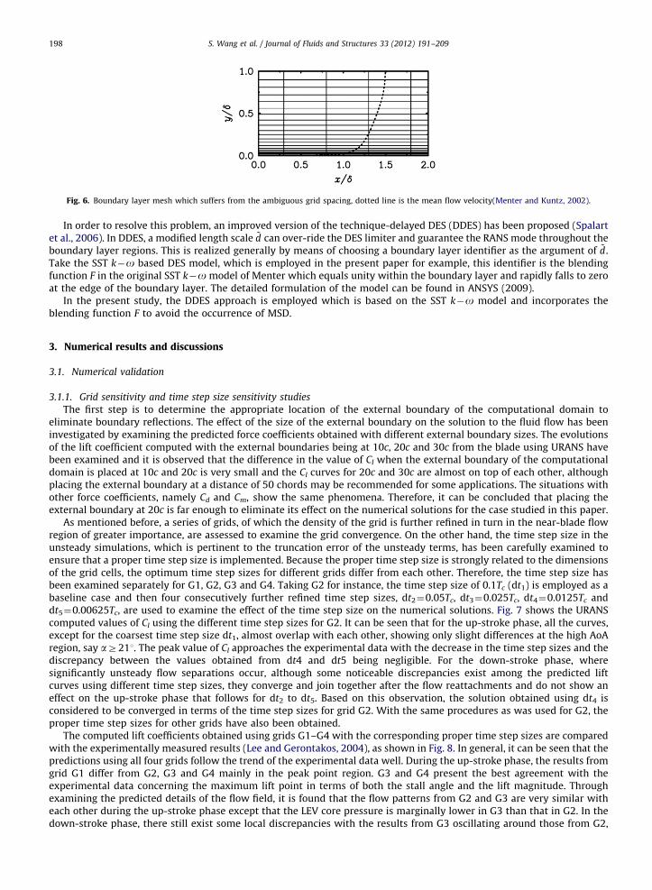
Fig. 6. Boundary layer mesh which suffers from the ambiguous grid spacing, dotted line is the mean flow velocity(Menter and Kuntz, 2002).


In order to resolve this problem, an improved version of the technique-delayed DES (DDES) has been proposed (Spalartet al., 2006). In DDES, a modified length scale ~d can over-ride the DES limiter and guarantee the RANS mode throughout theboundary layer regions. This is realized generally by means of choosing a boundary layer identifier as the argument of ~d.Take the SST k�o based DES model, which is employed in the present paper for example, this identifier is the blendingfunction F in the original SST k�o model of Menter which equals unity within the boundary layer and rapidly falls to zeroat the edge of the boundary layer. The detailed formulation of the model can be found in ANSYS (2009).

In the present study, the DDES approach is employed which is based on the SST k�o model and incorporates theblending function F to avoid the occurrence of MSD.

3. Numerical results and discussions

3.1. Numerical validation

3.1.1. Grid sensitivity and time step size sensitivity studies

The first step is to determine the appropriate location of the external boundary of the computational domain toeliminate boundary reflections. The effect of the size of the external boundary on the solution to the fluid flow has beeninvestigated by examining the predicted force coefficients obtained with different external boundary sizes. The evolutionsof the lift coefficient computed with the external boundaries being at 10c, 20c and 30c from the blade using URANS havebeen examined and it is observed that the difference in the value of Cl when the external boundary of the computationaldomain is placed at 10c and 20c is very small and the Cl curves for 20c and 30c are almost on top of each other, althoughplacing the external boundary at a distance of 50 chords may be recommended for some applications. The situations withother force coefficients, namely Cd and Cm, show the same phenomena. Therefore, it can be concluded that placing theexternal boundary at 20c is far enough to eliminate its effect on the numerical solutions for the case studied in this paper.

As mentioned before, a series of grids, of which the density of the grid is further refined in turn in the near-blade flowregion of greater importance, are assessed to examine the grid convergence. On the other hand, the time step size in theunsteady simulations, which is pertinent to the truncation error of the unsteady terms, has been carefully examined toensure that a proper time step size is implemented. Because the proper time step size is strongly related to the dimensionsof the grid cells, the optimum time step sizes for different grids differ from each other. Therefore, the time step size hasbeen examined separately for G1, G2, G3 and G4. Taking G2 for instance, the time step size of 0.1Tc (dt1) is employed as abaseline case and then four consecutively further refined time step sizes, dt2¼0.05Tc, dt3¼0.025Tc, dt4¼0.0125Tc anddt5¼0.00625Tc, are used to examine the effect of the time step size on the numerical solutions. Fig. 7 shows the URANScomputed values of Cl using the different time step sizes for G2. It can be seen that for the up-stroke phase, all the curves,except for the coarsest time step size dt1, almost overlap with each other, showing only slight differences at the high AoAregion, say aZ211. The peak value of Cl approaches the experimental data with the decrease in the time step sizes and thediscrepancy between the values obtained from dt4 and dt5 being negligible. For the down-stroke phase, wheresignificantly unsteady flow separations occur, although some noticeable discrepancies exist among the predicted liftcurves using different time step sizes, they converge and join together after the flow reattachments and do not show aneffect on the up-stroke phase that follows for dt2 to dt5. Based on this observation, the solution obtained using dt4 isconsidered to be converged in terms of the time step sizes for grid G2. With the same procedures as was used for G2, theproper time step sizes for other grids have also been obtained.

The computed lift coefficients obtained using grids G1–G4 with the corresponding proper time step sizes are comparedwith the experimentally measured results (Lee and Gerontakos, 2004), as shown in Fig. 8. In general, it can be seen that thepredictions using all four grids follow the trend of the experimental data well. During the up-stroke phase, the results fromgrid G1 differ from G2, G3 and G4 mainly in the peak point region. G3 and G4 present the best agreement with theexperimental data concerning the maximum lift point in terms of both the stall angle and the lift magnitude. Throughexamining the predicted details of the flow field, it is found that the flow patterns from G2 and G3 are very similar witheach other during the up-stroke phase except that the LEV core pressure is marginally lower in G3 than that in G2. In thedown-stroke phase, there still exist some local discrepancies with the results from G3 oscillating around those from G2,

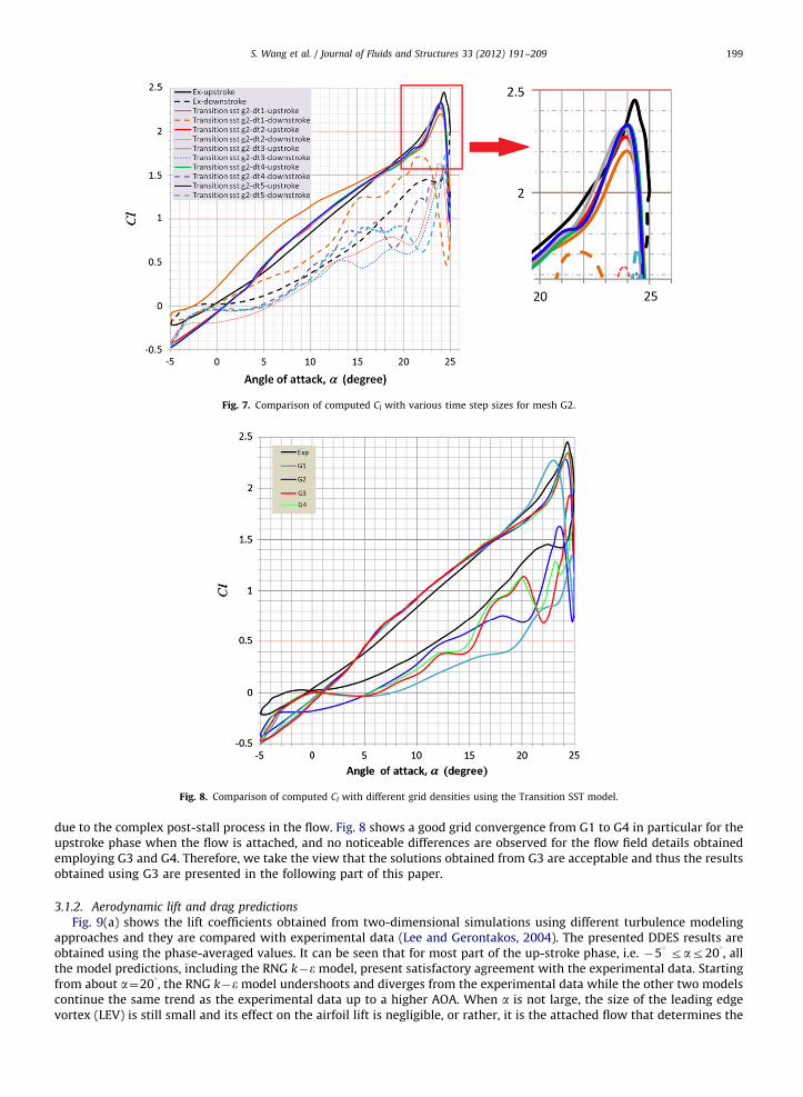
Fig. 7. Comparison of computed Cl with various time step sizes for mesh G2.

Fig. 8. Comparison of computed Cl with different grid densities using the Transition SST model.


due to the complex post-stall process in the flow. Fig. 8 shows a good grid convergence from G1 to G4 in particular for theupstroke phase when the flow is attached, and no noticeable differences are observed for the flow field details obtainedemploying G3 and G4. Therefore, we take the view that the solutions obtained from G3 are acceptable and thus the resultsobtained using G3 are presented in the following part of this paper.

3.1.2. Aerodynamic lift and drag predictions

Fig. 9(a) shows the lift coefficients obtained from two-dimensional simulations using different turbulence modelingapproaches and they are compared with experimental data (Lee and Gerontakos, 2004). The presented DDES results areobtained using the phase-averaged values. It can be seen that for most part of the up-stroke phase, i.e. �51 rar201, allthe model predictions, including the RNG k�e model, present satisfactory agreement with the experimental data. Startingfrom about a¼201, the RNG k�e model undershoots and diverges from the experimental data while the other two modelscontinue the same trend as the experimental data up to a higher AOA. When a is not large, the size of the leading edgevortex (LEV) is still small and its effect on the airfoil lift is negligible, or rather, it is the attached flow that determines the

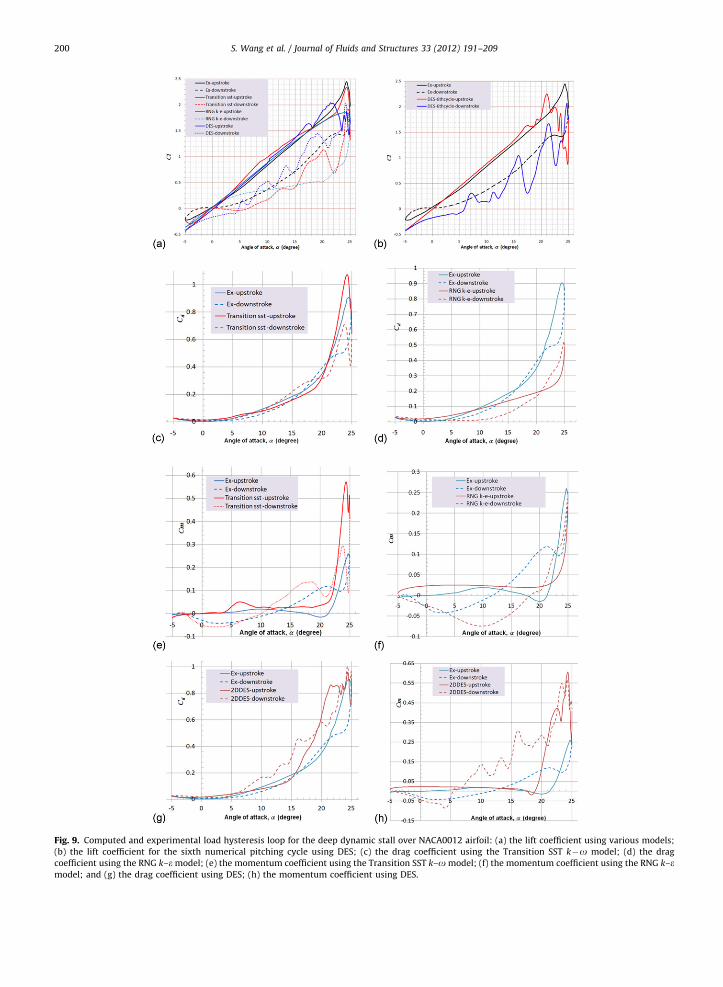
Fig. 9. Computed and experimental load hysteresis loop for the deep dynamic stall over NACA0012 airfoil: (a) the lift coefficient using various models;

(b) the lift coefficient for the sixth numerical pitching cycle using DES; (c) the drag coefficient using the Transition SST k�o model; (d) the drag

coefficient using the RNG k–e model; (e) the momentum coefficient using the Transition SST k–o model; (f) the momentum coefficient using the RNG k–emodel; and (g) the drag coefficient using DES; (h) the momentum coefficient using DES.



lift. Therefore, it does not matter much whether the development of the LEV is well captured or not at this stage. However,when a is large, and the LEV grows bigger, the pressure suction wave carried by the LEV will take charge. Apparently, theRNG k�e model failed to resolve the LEV and therefore the predicted flow actually progressed into the trailing edge stalldirectly. The other models are able to predict the LEV and therefore continue to have better agreement with experimentaldata at large AOAs.

The predicted lift stall occurs at aE23.81 and 211 for the Transition SST model and the averaged 2-D DDES results,respectively. However, the Transition SST model presents a too sharp drop-off of Cl shortly after the lift stall occurs (ClE0.7at a¼251), thus presenting an over-prediction of the intensity of the stall which significantly affects the prediction of thesubsequent flow-reattachment in the down-stroke phase. The DDES predicted Cl from the 6th computed oscillating cycleare compared with the experimental data in Fig. 9(b). It shows a very good agreement during the up-stroke at low anglesof attack until aE201. The Cl curves from different oscillating cycles collapse with each other for this range of low AOA (forclarity, only the curves for the 6th calculation cycle is displayed in Fig. 9(b)). This reveals a feature of flow periodicity underthis low AOA region. For the rest of the up-stroke phase, and most of the down-stroke phase, the computed values of Cl

from DDES present a strong oscillating behavior which differs from cycle to cycle. This non-periodical flow feature is likelydue to the existence of the complex and intensive unsteady flow separations being captured even with a 2-D DEScalculation. The fluctuated aerodynamic loads obtained from the DES method are consistent with the flow physics revealedby experimental data (Geissler et al., 2007) in terms of the significant differences in the aerodynamic loads observedamong different pitching cycles, and this was not captured by the adopted URANS methods. However, it is noted that the2-D DES predicted stall point is approximately 0.81 earlier than that was observed in the experiments and the predictedpeak value of Cl is also smaller than the reported experimental value.

In general, the prediction for the up-stroke phase using the URANS with the Transition SST model is in fairly goodagreement with the experimental data in that the delay of the stall is captured reasonably well. In contrast, the predictionsof the down-stroke phase by both URANS models are not in good agreement with experimental data due to thecomplicated post-stall flow structures which the URANS turbulence models failed to capture well. Although the TransitionSST model present a very sharp drop-off of the lift coefficient when the airfoil approaches the maximum angle of attack,the computed lift from the Transition SST model jumps back quickly and then follows the tendency of the experimentalcurve well when ar151. Due to large separations when the AOA is close to its maxima, and for a large portion of thedown-stroke phase, the computed curves from different oscillating cycles in 2-D DES deviate from each other and presenta wide area of distribution until they collapse with each other at the end of the down-stroke phase. This phenomena wasalso reported by Geissler et al. (2007). Nevertheless, although the 2-D DES presents a fluctuated prediction of the lift forcefrom blade oscillating cycle to cycle for the down-stroke, averaged values of Cl from the consecutive cycles presents a fairlygood consistency with the experimental data, which is actually averaged as well, except in the small region �51rar51, asillustrated in Fig. 9(a) and (b). This suggests that the capacity of DES in resolving large turbulence eddies plays animportant role in capture the unsteadiness of the separated flows at deep stall conditions in the down-stroke phase, whistthe RANS is incapable of doing it.

The simulated drag and momentum coefficients are shown in Fig. 9(c)–(h). The value of Cd obtained by the TransitionSST model is generally in good agreement with the experimental data, see Fig. 9(c), while the RNG k–e model gives asignificant undershoot, and the 2-D DES averaged Cd presents an overshoot for both up-stroke (151rar251) and down-stroke phases, see Fig. 8(d) and (g), respectively. It has to be noted that the shape of the Cd curve from the DES is in quitegood agreement with the reported experimental data, despite the over-prediction at the high AoAs. In terms of Cm,

although the peak value of Cm at the onset of the stall is greatly over-predicted by the Transition SST model, as well as the2-D DES, the tendency of the predicted Cm curves still agree well with the experimental data, as are shown in Fig. 8(e) and(h). The predictions of Cm from the RNG k–e model are in general reasonable as well, see Fig. 9(f).

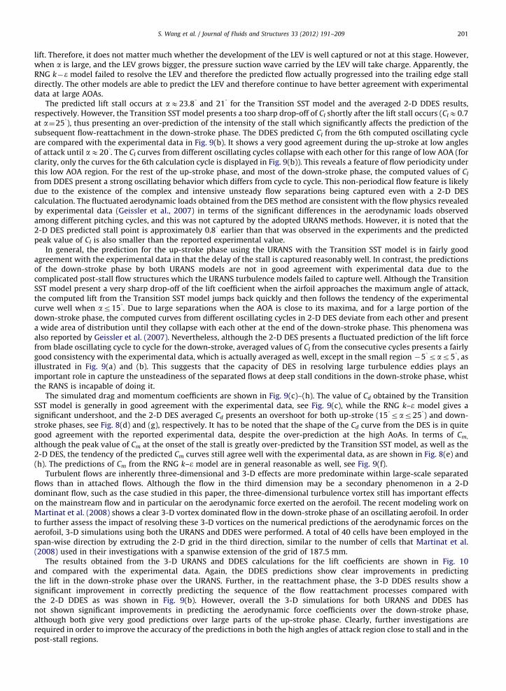
Turbulent flows are inherently three-dimensional and 3-D effects are more predominate within large-scale separatedflows than in attached flows. Although the flow in the third dimension may be a secondary phenomenon in a 2-Ddominant flow, such as the case studied in this paper, the three-dimensional turbulence vortex still has important effectson the mainstream flow and in particular on the aerodynamic force exerted on the aerofoil. The recent modeling work onMartinat et al. (2008) shows a clear 3-D vortex dominated flow in the down-stroke phase of an oscillating aerofoil. In orderto further assess the impact of resolving these 3-D vortices on the numerical predictions of the aerodynamic forces on theaerofoil, 3-D simulations using both the URANS and DDES were performed. A total of 40 cells have been employed in thespan-wise direction by extruding the 2-D grid in the third direction, similar to the number of cells that Martinat et al.(2008) used in their investigations with a spanwise extension of the grid of 187.5 mm.

The results obtained from the 3-D URANS and DDES calculations for the lift coefficients are shown in Fig. 10and compared with the experimental data. Again, the DDES predictions show clear improvements in predictingthe lift in the down-stroke phase over the URANS. Further, in the reattachment phase, the 3-D DDES results show asignificant improvement in correctly predicting the sequence of the flow reattachment processes compared withthe 2-D DDES as was shown in Fig. 9(b). However, overall the 3-D simulations for both URANS and DDES hasnot shown significant improvements in predicting the aerodynamic force coefficients over the down-stroke phase,although both give very good predictions over large parts of the up-stroke phase. Clearly, further investigations arerequired in order to improve the accuracy of the predictions in both the high angles of attack region close to stall and in thepost-stall regions.

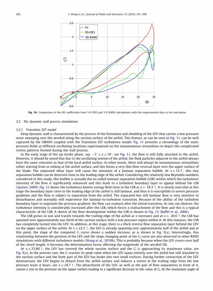
Fig. 10. Comparison of the lift coefficients from 3-D DES and 3-D RANS calculations with the experimental data at the mid-plane.


3.2. The dynamic stall process simulations

3.2.1. Transition SST model

Deep dynamic stall is characterized by the process of the formation and shedding of the LEV that carries a low pressurewave sweeping over the aerofoil along the suction surface of the airfoil. This feature, as can be seen in Fig. 11, can be wellcaptured by the URANS coupled with the Transition SST turbulence model. Fig. 11 presents a chronology of the staticpressure fields at different oscillating locations superimposed on the instantaneous streamlines to depict the complicatedvortex patterns formed during the stall process.

In the early stage of the up-stroke phase, say �51rar101, see Fig. 11, the flow is still fully attached to the airfoil.However, it should be noted that due to the oscillating motion of the airfoil, the fluid particles adjacent to the airfoil alwayshave the same velocities as that of the local airfoil surface. In other words, there will always be instantaneous streamlineseither starting from or ending at the airfoil surface, and this forms a very thin flow reversal layer over the upper surface ofthe blade. The separated shear layer will cause the initiation of a laminar separation bubble. At aE15.71, this tinyseparation bubble can be detected close to the leading edge of the airfoil. Considering the relatively low Reynolds numbersconsidered in this study, this bubble is actually the so-called laminar separation bubble (LSB) within which the turbulenceintensity of the flow is significantly enhanced and this leads to a turbulent boundary layer to appear behind the LSB(Spalart, 2000). Fig. 12 shows the turbulence kinetic energy field close to the LSB at aE 18.31m. It is clearly seen that at thisstage the boundary layer close to the leading edge of the airfoil is still laminar, and thus it is susceptible to severe pressuregradients and the flow is subject to separation from the airfoil. The separated but still laminar flow is very sensitive todisturbances and normally will experience the laminar-to-turbulent transition. Because of the ability of the turbulentboundary layer to negotiate the pressure gradient, the flow can reattach after the initial transition. As one can observe, theturbulence intensity is considerably increased after the LSB, which forces a reattachment of the flow and this is a typicalcharacteristic of the LSB. A sketch of the flow development within the LSB is shown in Fig. 13 (Raffel et al., 2006).

The LSB grows in size and travels towards the trailing edge of the airfoil as a increases and at aE 20.61m the LSB hasspanned over approximately one-third of the suction surface with a low pressure region within it. At this instance, the LSBhas completely turned into the LEV. In addition, at this stage, there is a thick reverse flow separation layer behind the LEVon the upper surface of the airfoil. At aE22.51m, the LEV is already spanning over approximately half of the airfoil and atthis point, the slope of the computed Cl curve shows a sudden increase, as is shown in Fig. 9(a). Interestingly, thisrelationship between the position of the LEV and the slope changing point of the Cl curve are also observed in other RANSsimulations with different turbulence models (Wang et al., 2010b). This is probably because when the LEV covers over halfof the chord length, it becomes the determination factor affecting the magnitude of the aerofoil lift.

At aE23.861m, the LEV has covered the whole suction surface and the Cl is approaching its maximum value, seeFig. 9(a). In the present case, the Cl reaches its peak value when the LEV spans entirely over the airfoil but still attached tothe suction surface and the front part of the LEV has broke into two small vortices. During further convection of the LEVdownstream, the LEV begins to detach from the airfoil surface and induces a vortex at the trailing edge from the lowpressure wave it bears, see aE24.71m. The detachment of the LEV, as well as the pair of flow separations in front of it,causes a rise in the pressure on the upper surface leading to a significant decrease in the value of Cl. At the maximum angle of

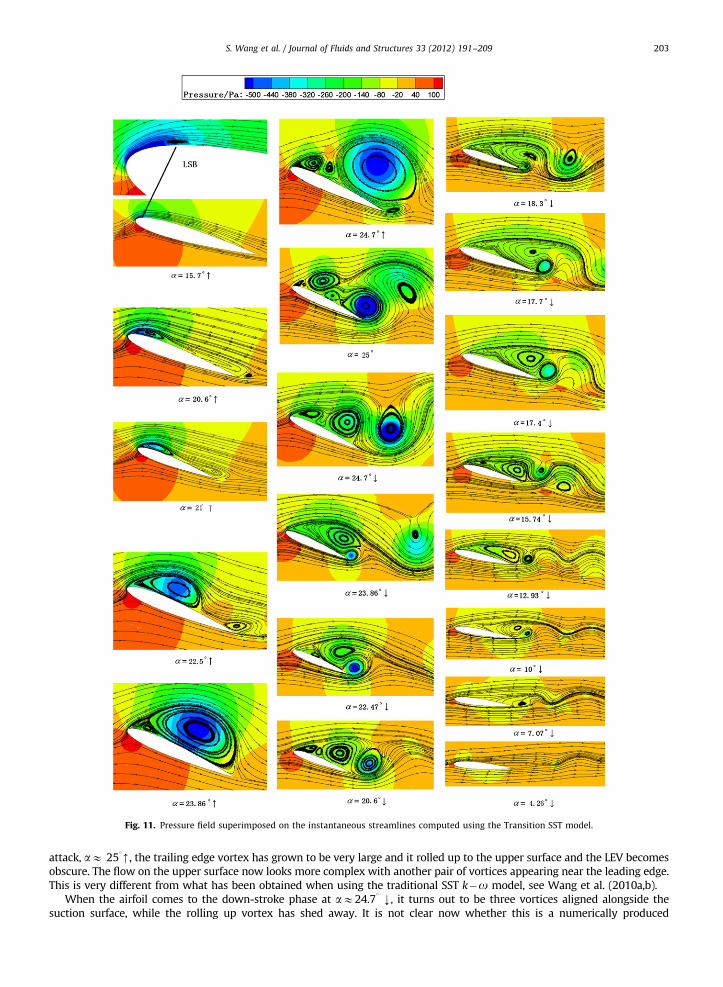
Fig. 11. Pressure field superimposed on the instantaneous streamlines computed using the Transition SST model.


attack, aE 251m, the trailing edge vortex has grown to be very large and it rolled up to the upper surface and the LEV becomesobscure. The flow on the upper surface now looks more complex with another pair of vortices appearing near the leading edge.This is very different from what has been obtained when using the traditional SST k�o model, see Wang et al. (2010a,b).

When the airfoil comes to the down-stroke phase at aE24.71 k, it turns out to be three vortices aligned alongside thesuction surface, while the rolling up vortex has shed away. It is not clear now whether this is a numerically produced

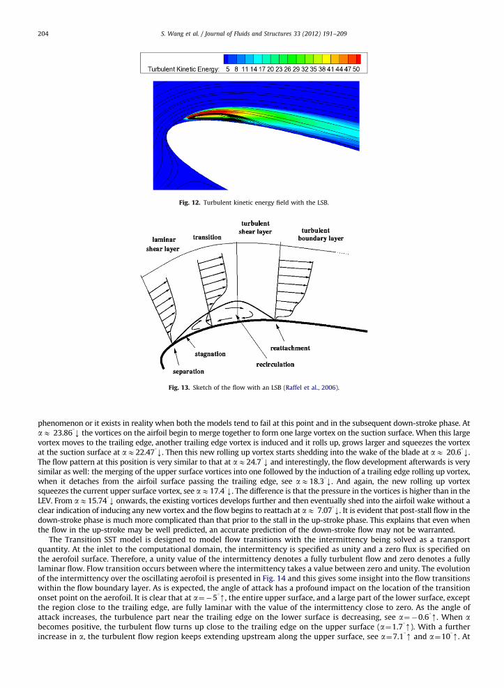
Fig. 12. Turbulent kinetic energy field with the LSB.

Fig. 13. Sketch of the flow with an LSB (Raffel et al., 2006).


phenomenon or it exists in reality when both the models tend to fail at this point and in the subsequent down-stroke phase. AtaE 23.861k the vortices on the airfoil begin to merge together to form one large vortex on the suction surface. When this largevortex moves to the trailing edge, another trailing edge vortex is induced and it rolls up, grows larger and squeezes the vortexat the suction surface at aE22.471k. Then this new rolling up vortex starts shedding into the wake of the blade at aE 20.61k.The flow pattern at this position is very similar to that at aE24.71k and interestingly, the flow development afterwards is verysimilar as well: the merging of the upper surface vortices into one followed by the induction of a trailing edge rolling up vortex,when it detaches from the airfoil surface passing the trailing edge, see aE18.31k. And again, the new rolling up vortexsqueezes the current upper surface vortex, see aE17.41k. The difference is that the pressure in the vortices is higher than in theLEV. From aE15.741k onwards, the existing vortices develops further and then eventually shed into the airfoil wake without aclear indication of inducing any new vortex and the flow begins to reattach at aE 7.071k. It is evident that post-stall flow in thedown-stroke phase is much more complicated than that prior to the stall in the up-stroke phase. This explains that even whenthe flow in the up-stroke may be well predicted, an accurate prediction of the down-stroke flow may not be warranted.

The Transition SST model is designed to model flow transitions with the intermittency being solved as a transportquantity. At the inlet to the computational domain, the intermittency is specified as unity and a zero flux is specified onthe aerofoil surface. Therefore, a unity value of the intermittency denotes a fully turbulent flow and zero denotes a fullylaminar flow. Flow transition occurs between where the intermittency takes a value between zero and unity. The evolutionof the intermittency over the oscillating aerofoil is presented in Fig. 14 and this gives some insight into the flow transitionswithin the flow boundary layer. As is expected, the angle of attack has a profound impact on the location of the transitiononset point on the aerofoil. It is clear that at a¼�51m, the entire upper surface, and a large part of the lower surface, exceptthe region close to the trailing edge, are fully laminar with the value of the intermittency close to zero. As the angle ofattack increases, the turbulence part near the trailing edge on the lower surface is decreasing, see a¼�0.61m. When abecomes positive, the turbulent flow turns up close to the trailing edge on the upper surface (a¼1.71m). With a furtherincrease in a, the turbulent flow region keeps extending upstream along the upper surface, see a¼7.11m and a¼101m. At

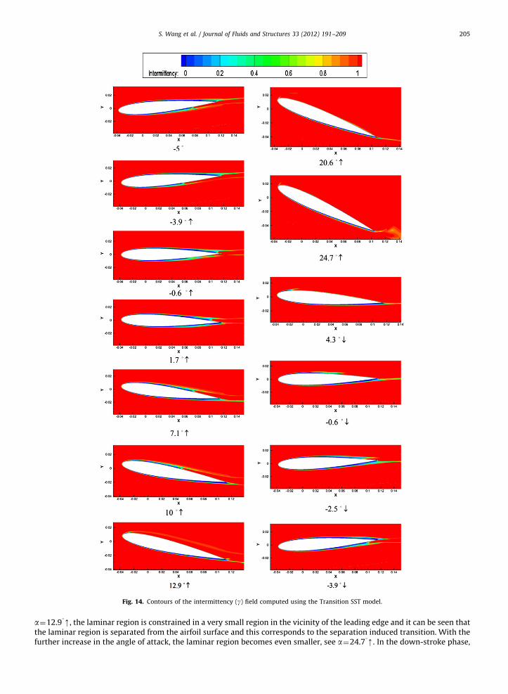
Fig. 14. Contours of the intermittency (g) field computed using the Transition SST model.


a¼12.91m, the laminar region is constrained in a very small region in the vicinity of the leading edge and it can be seen thatthe laminar region is separated from the airfoil surface and this corresponds to the separation induced transition. With thefurther increase in the angle of attack, the laminar region becomes even smaller, see a¼24.71m. In the down-stroke phase,


with the decrease in a, the laminar region begins to increase. It should be noted that the re-laminarization process in thedown-stroke part lags behind that in the up-stroke and the upper surface is not fully re-laminarized even until a¼�2.51k.

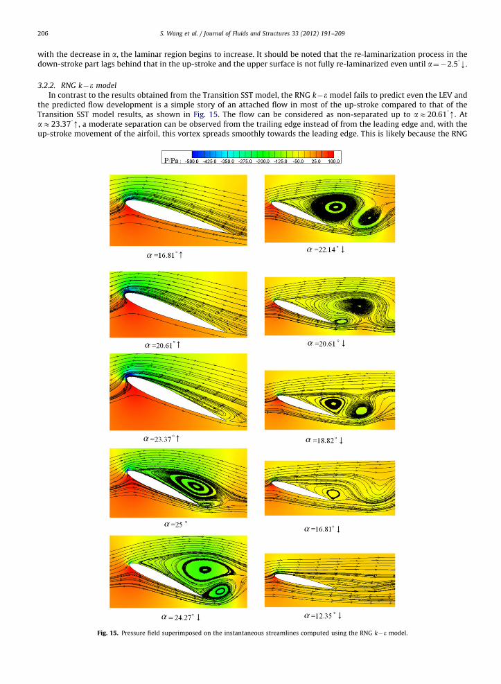
3.2.2. RNG k�e model

In contrast to the results obtained from the Transition SST model, the RNG k�e model fails to predict even the LEV andthe predicted flow development is a simple story of an attached flow in most of the up-stroke compared to that of theTransition SST model results, as shown in Fig. 15. The flow can be considered as non-separated up to aE20.611m. AtaE23.371m, a moderate separation can be observed from the trailing edge instead of from the leading edge and, with theup-stroke movement of the airfoil, this vortex spreads smoothly towards the leading edge. This is likely because the RNG

Fig. 15. Pressure field superimposed on the instantaneous streamlines computed using the RNG k�e model.


k�e model is still too diffusive as it is for the standard k�e model and it fails to predict the adverse pressure gradientleading to the LEV. At aE251m, the separation has spanned the entire suction surface of the airfoil and, as expected, asecondary trailing edge vortex is induced by the large separation. Since the flow separation does not originate from an LSBtherefore the observed vortex over the suction surface is merely a high pressure whirling flow and this results in theunder-prediction of the lift coefficient for 181rar251. In addition, a flow pattern of Karman Vortex Street type can beobserved during the down-stroke phase in which vortices generated from the upper and lower surfaces shed alternatively.

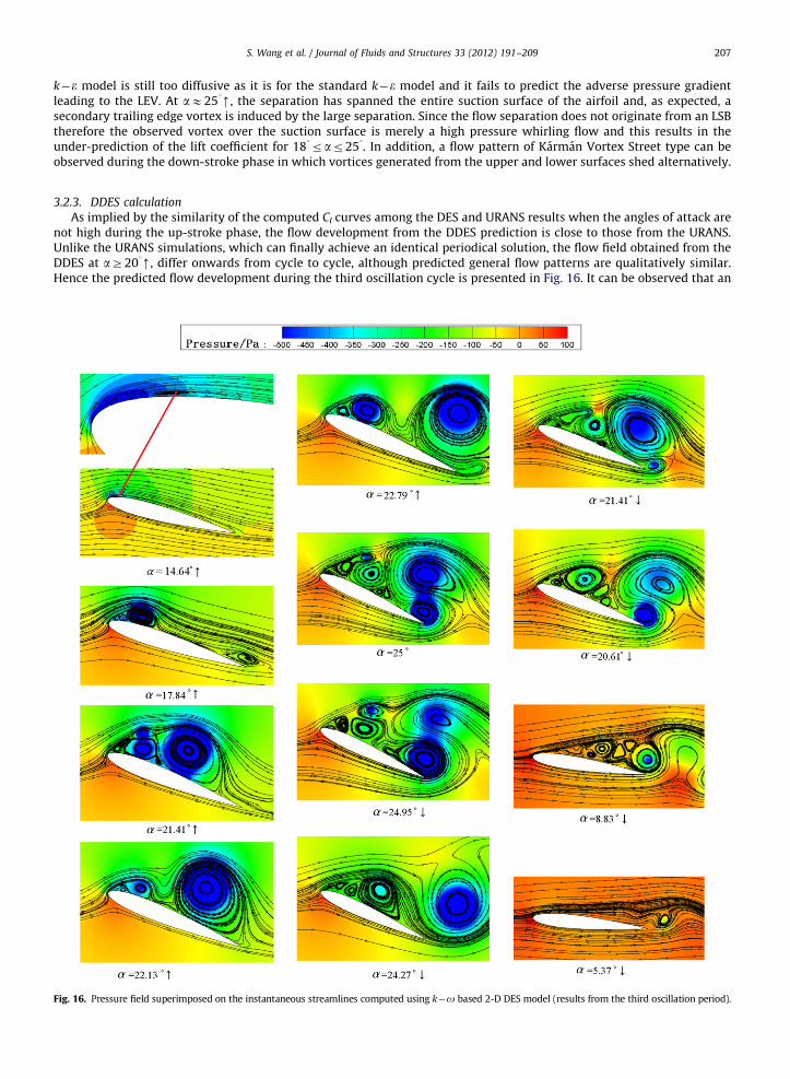
3.2.3. DDES calculation

As implied by the similarity of the computed Cl curves among the DES and URANS results when the angles of attack arenot high during the up-stroke phase, the flow development from the DDES prediction is close to those from the URANS.Unlike the URANS simulations, which can finally achieve an identical periodical solution, the flow field obtained from theDDES at aZ201m, differ onwards from cycle to cycle, although predicted general flow patterns are qualitatively similar.Hence the predicted flow development during the third oscillation cycle is presented in Fig. 16. It can be observed that an

Fig. 16. Pressure field superimposed on the instantaneous streamlines computed using k�o based 2-D DES model (results from the third oscillation period).


LSB appeared at aE14.641m which is slightly earlier than is predicted by the URANS with the Transition SST model. Itshould be noted that a trailing edge vortex forms at aE17.841m, which is observed instead of at aE211m from the URANSTransition SST simulation. Clearly this trailing edge vortex is not induced by the LEV but due to the rapid flap motion of thetrailing edge. In addition, another pair of secondary vortices occur from the leading edge and at aE21.411m they havegrown to be almost as large as the LEV. However, they dissipate very quickly and become very weak at aE22.131m. TheLEV separates from the airfoil at aE22.791m and this corresponds to the decrease in the Cl at this AOA. Because theshedding of the LEV occurs at a relatively low angle of attack, this provides the opportunity for a series of additionalsecondary vortices to form at the leading edge during the subsequent up-stroke motion of the airfoil, and these vorticestravel along the suction surface of the airfoil causing strong unsteadiness of the aerodynamic loads on the airfoil. Further,since these vortices possess local low pressure waves when they are generated at the leading edge, they actually functionlike the LEV, although their strength is not as strong.

In general, the DDES, even in its 2-D application, calculation presents much more complicated flow structures, involvinga more complex system of vortices. It can be deduced that it is this continuous generation and shedding of these vorticesthat cause the fluctuating in the computed value of Cl. It is considered unnecessary and too wordy to detail the sequencesof the flow developments presented in Fig. 16 and the plots are quite self-explanatory. In particular, it is suggested thatmore information from experimental investigations is required to validate and subsequently explain these complexpredicted scenarios. Nevertheless, it should be noted that the predicted flow structures from DES for the down-strokephase produce a lift curve that is in good agreement, in general, with the experiment data whilst the RANS fail to achievethis for the case studied.

4. Conclusions

In this paper, URANS, incorporating both the RNG k�e and the Transition SST models and DDES based on the SST k�omodel have been employed in order to simulate the fluid flow over a NACA 0012 airfoil that is executing a sinusoidalpitching motion, in the relatively low Reynolds number regime of the order 105. The case studied involves deep dynamicstall that is comparable to the dynamic stall typically occurring in the operation of small-to-medium sized wind turbines,especially the VAWTs. The instantaneous aerodynamic loads exerted on the airfoil, and the associated flow structurearound the airfoil, including boundary layer transitions have been numerically revealed.

The results show that there is a strong correlation between the lift coefficient curve and the development of the LEV forthe specific case studied, i.e. (1) the slope change point: when the LEV spans about a half of the chord length, there will bea significant increase in the slope of the lift curve; and (2) the peak point: when the LEV spans the whole chord length butit is still attached to the blade, the lift culminates. Since the LEV originates from the LSB, the accurate modeling of theboundary layer transition process is crucial in simulating the low Re dynamic stall phenomena.

For the case studied, the RNG k�e model cannot produce the LEV and suggests a trailing edge stall, and thus cannotqualitatively reveal the leading edge stall mechanism of the studied dynamic stall phenomena. In general, although the2-D Transition SST model employed predicts a slightly undershoot at the maximum lift point, it still can predict theexperimental data with reasonable accuracy for most of the up-stroke phase. A qualitatively reasonable prediction of thelift for the complicated separated flows during the reattachment/down-stroke phase is still achieved, in spite of the over-prediction of the lift loss at the stall point.

The SST k�o based DDES presents generally good agreement with the experimental data, especially for the down-stroke phase compared with the URANS with the Transition SST model. In addition, DDES solutions reveal a periodical flowpattern, as URANS does for low angles of attack in the up-stroke phase from oscillating cycle to cycle. However, thepredicted flow becomes non-periodical for large angles of attack and in the down-stroke phase, which the URANS solutionsdid not present. The tendency of the computed Cd and Cm curves from DDES are in good agreement with the experimentaldata. However, DDES predicts a slightly earlier stall point than that observed in the experiment and it fails to capture thepeak of the lift coefficient for the case studied.

The results show significant 3-D effects when the angle of attack reaches high values and in the down-stroke phase. The3-D simulations have not shown substantial improvements over 2-D simulations in terms of predicting the lift forcecoefficients in the case studied. Clearly, further investigations are required in order to more accurately predict theaerodynamic forces on the aerofoil pertinent to wind turbine applications.

Acknowledgments

The authors would like to acknowledge the financial support from the Chinese Scholarship Council (CSC) for thisresearch. Also the authors would like to express their gratitude to Professor T. Lee from McGill University, Canada, DoctorK. Richter from DLR, Gottingen, Germany, for offering useful information and constructive comments on the experimentalstudies employed in this paper.


References

Aleksey, G., 2007. LES & DES in FLUENT. ANSYS training material.Amiralaei, M.R., Alighanbari, H., Hashemi, S.M., 2010. An investigation into the effects of unsteady parameters on the aerodynamics of a low Reynolds

number pitching airfoil. Journal of Fluids and Structures 26, 979–993.ANSYS, 2009. ANSYS FLUENT 12.0 Theory Guide. Ansys Inc., USA.Carr, L., 1988. Progress in analysis and prediction of dynamic stall. Journal of Aircraft 25, 6–17.Ericsson, L.E., Reding, J.P., 1988. Fluid mechanics of dynamic stall part I. Unsteady flow concepts. Journal of Fluids and Structures. 2, 1–33.Fraunie, P., Beguier, C., Paraschivoiu, I., Brochier, G., 1986. Water channel experiments of dynamic stall on Darrieus wind turbine blades. Journal of

Propulsion and Power 2, 445–449.Galvanetto, U., Peiro, J., Chantharasenawong, C., 2008. An assessment of some effects of the nonsmoothness of the Leishman–Beddoes dynamic stall

model on the nonlinear dynamics of a typical aerofoil section. Journal of Fluids and Structures 24, 151–163.Geissler, W., Raffel, M., Dietz, G., Mai, H., 2007. Helicopter aerodynamics with emphasis placed on dynamic stall. In: Peinke, J., Schaumann, P., Barth, S.

(Eds.), Wind Energy, Springer, Berlin, Heidelberg, pp. 199–204.Hansen, A., Butterfield, C., 1993. Aerodynamics of horizontal-axis wind turbines. Annual Review of Fluid Mechanics. 25, 115–149.Lee, T., Gerontakos, P., 2004. Investigation of flow over an oscillating airfoil. Journal of Fluid Mechanics 512, 313–341.Leishman, J., 2006. Principles of Helicopter Aerodynamics, second ed. Cambridge Univ Press, Cambridge.Martinat, G., Braza, M., Hoarau, Y., Harran, G., 2008. Turbulence modelling of the flow past a pitching NACA0012 airfoil at 105 and 106 Reynolds numbers.

Journal of Fluids and Structures 24, 1294–1303.McCroskey, W., Carr, L., McAlister, K., 1976. Dynamic stall experiments on oscillating airfoils. AIAA Journal 14, 57–63.McCroskey, W., McAlister, K., Carr, L., Pucci, S., 1982. An Experimental Study of Dynamic Stall on Advanced Airfoil Sections. Volume 1: Summary of the

Experiment. NASA TM.McLaren, K., Tullis, S., Ziada, S., Measurement of high solidity vertical axis wind turbine aerodynamic loads under high vibration response conditions.

Journal of Fluids and Structures, http://dx.doi.org/10.1016/j.jfluidstructs.2012.01.001, in press.Menter, F.R., 1994. Two-equation eddy-viscosity turbulence models for engineering applications. AIAA Journal 32, 1598–1605.Menter, F., Kuntz, M., 2002. Adaptation of Eddy Viscosity Turbulence Models to Unsteady Separated Flow Behind Vehicles. Springer, Germany.Menter, F.R., Langtry, R., VolKer, S., 2006. Transition modelling for general purpose CFD codes. Flow, Turbulence and Combustion 77, 277–303.Mohamed, K., Nadarajah, S., Paraschivoiu, M., 2009. Detached-eddy simulation of a wing tip vortex at dynamic stall conditions. Journal of Aircraft 46,

1302–1313.Paul, E., Atiemo-Obeng, V., Kresta, S., 2004. Handbook of Industrial Mixing: Science and Practice. John Wiley & Sons, Inc., Hoboken, New Jersey.Poirel, D., Metivier, V., Dumas, G., 2011. Computational aeroelastic simulations of self-sustained pitch oscillations of a NACA0012 at transitional Reynolds

numbers. Journal of Fluids and Structures 27, 1262–1277.Raffel, M., Favier, D., Berton, E., Rondot, C., Nsimba, M., Geissler, W., 2006. Micro-PIV and ELDV wind tunnel investigations of the laminar separation

bubble above a helicopter blade tip. Measurement Science and Technology 17, 1652–1658.Sheldahl, R., Klimas, P., Feltz, L., 1980. Aerodynamic Performance of a 5-Meter-Diameter Darrieus Turbine with Extruded Aluminum NACA 0015 Blades.

Sandia Laboratories, Albuquerque, New Mexico, USA.Spalart, P., 2000. Strategies for turbulence modelling and simulations. International Journal of Heat and Fluid Flow 21, 252–263.Spalart, P., Deck, S., Shur, M., Squires, K., Strelets, M., Travin, A., 2006. A new version of detached-eddy simulation, resistant to ambiguous grid densities.

Theoretical and Computational Fluid Dynamics. 20, 181–195.Spentzos, A., Barakos, G., Badcock, K., Richards, B., Wernert, P., Schreck, S., Raffel, M., 2005. Investigation of three-dimensional dynamic stall using

computational fluid dynamics. AIAA Journal 43, 1023–1033.Wang, S., Ingham, D., Ma, L., Pourkashanian, M., Tao, Z., 2010a. Numerical investigations on dynamic stall of low Reynolds number flow around oscillating

airfoils. Computers & Fluids 39, 1529–1541.Wang, S., Tao, Z., Ma, L., Ingham, D., Pourkashanian, M., 2010b. Numerical investigations on dynamic stall associated with low Reynolds number flows

over airfoils. IEEE. 5 2nd International Conference on Computer Engineering and Technology, V5-308–312.Wernert, P., Geissler, W., Raffel, M., Kompenhans, J., 1996. Experimental and numerical investigations of dynamic stall on a pitching airfoil. AIAA Journal

34, 982–989.


Documents

Turbulence modeling of deep dynamic stall at relatively low Reynolds number