1

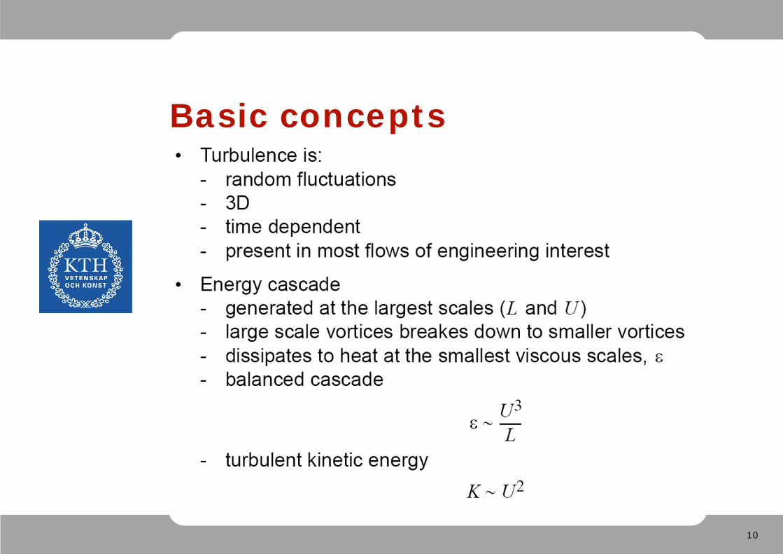
Turbulence

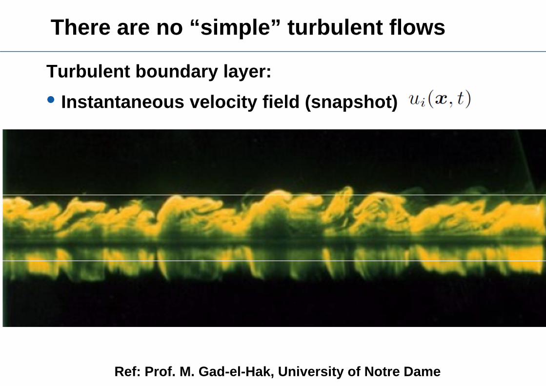
There are no “simple” turbulent flows

Turbulent boundary layer:• Instantaneous velocity field (snapshot)

Ref: Prof. M. Gad-el-Hak, University of Notre Dame

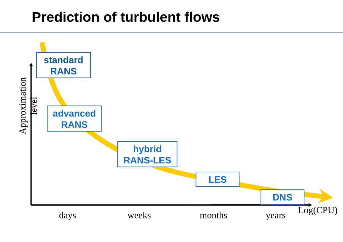
App

roxi

mat

ion

leve

l

Log(CPU)

advanced RANS

hybrid RANS-LES

LES

DNS

days weeks months years

standard RANS

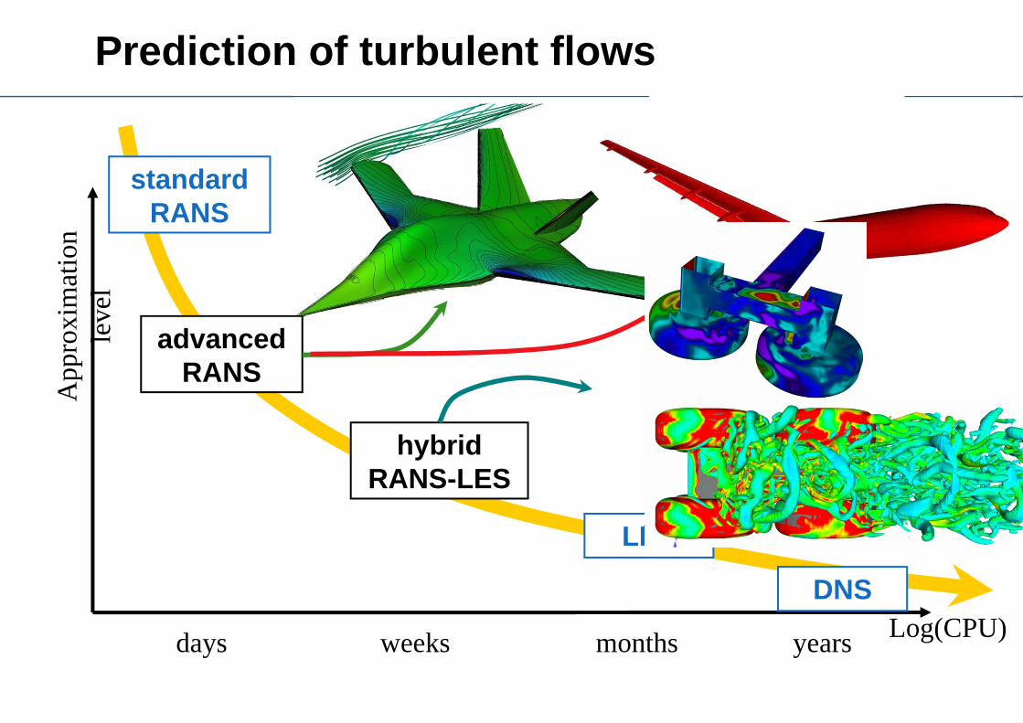
Prediction of turbulent flows

App

roxi

mat

ion

leve

l

Log(CPU)

advanced RANS

hybrid RANS-LES

LES

DNS

days weeks months years

standard RANS

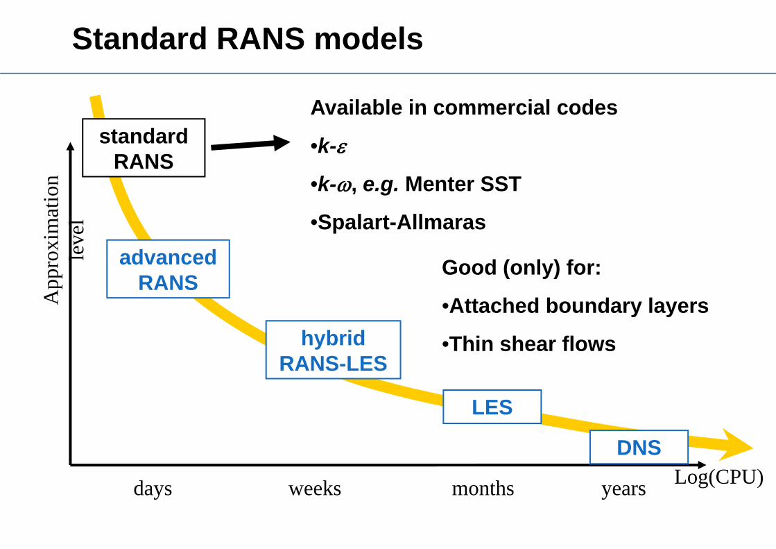
Standard RANS models

Available in commercial codes

•k-

•k-, e.g. Menter SST

•Spalart-Allmaras

Good (only) for:

•Attached boundary layers

•Thin shear flows

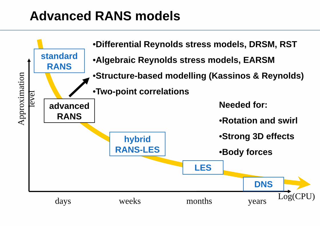
•Differential Reynolds stress models, DRSM, RST

•Algebraic Reynolds stress models, EARSM

•Structure-based modelling (Kassinos & Reynolds)

•Two-point correlations

App

roxi

mat

ion

leve

l

Log(CPU)

advanced RANS

hybrid RANS-LES

LES

DNS

days weeks months years

standard RANS

Advanced RANS models

Needed for:

•Rotation and swirl

•Strong 3D effects

•Body forces

App

roxi

mat

ion

leve

l

Log(CPU)

advanced RANS

hybrid RANS-LES

LES

DNS

days weeks months years

standard RANS

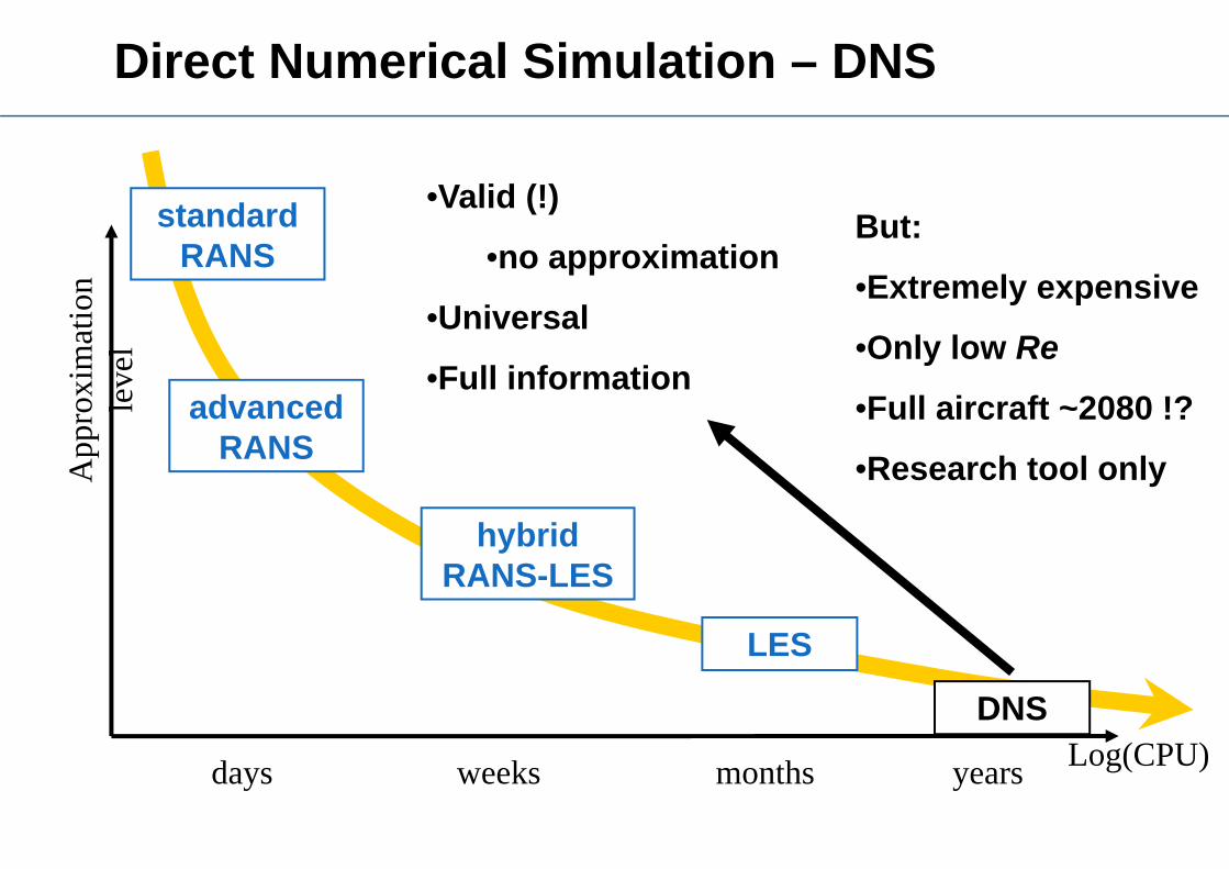
Direct Numerical Simulation – DNS

•Valid (!)

•no approximation

•Universal

•Full information

But:

•Extremely expensive

•Only low Re

•Full aircraft ~2080 !?

•Research tool only

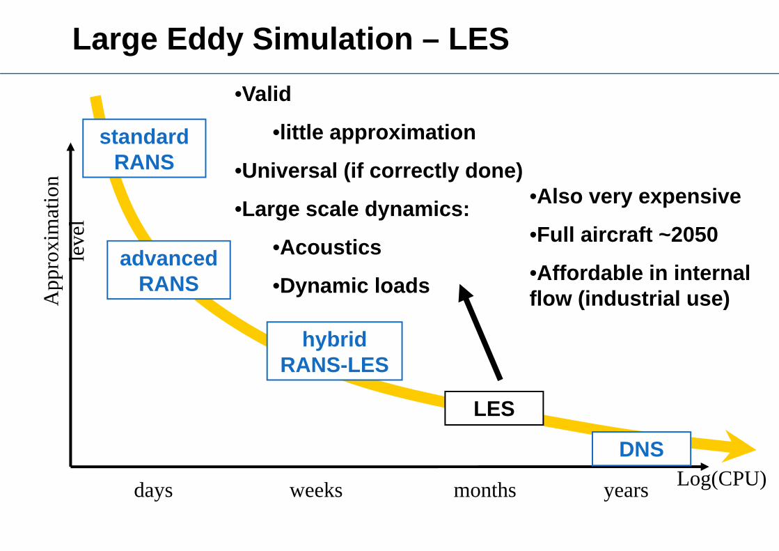
•Valid

•little approximation

•Universal (if correctly done)

•Large scale dynamics:

•Acoustics

•Dynamic loadsApp

roxi

mat

ion

leve

l

Log(CPU)

advanced RANS

hybrid RANS-LES

LES

DNS

days weeks months years

standard RANS

Large Eddy Simulation – LES

•Also very expensive

•Full aircraft ~2050

•Affordable in internal flow (industrial use)

App

roxi

mat

ion

leve

l

Log(CPU)

advanced RANS

hybrid RANS-LES

LES

DNS

days weeks months years

standard RANS

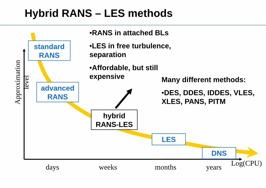
Hybrid RANS – LES methods•RANS in attached BLs

•LES in free turbulence, separation

•Affordable, but still expensive Many different methods:

•DES, DDES, IDDES, VLES, XLES, PANS, PITM

App

roxi

mat

ion

leve

l

Log(CPU)

advanced RANS

hybrid RANS-LES

LES

DNS

days weeks months years

standard RANS

Prediction of turbulent flows

10

Basic concepts

11

DNS

RANS

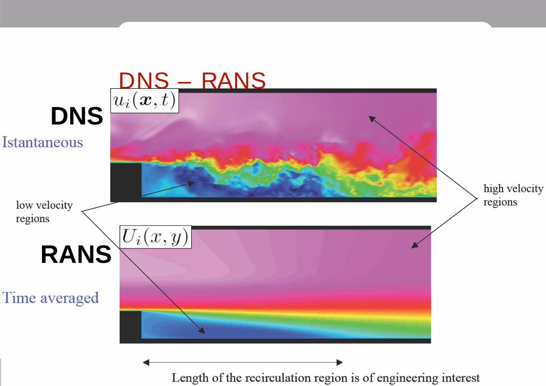
DNS – RANS

12

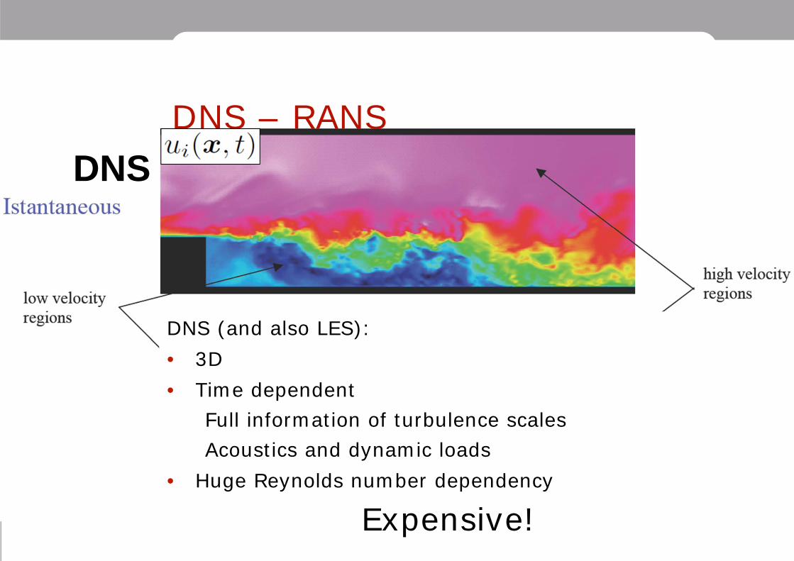
DNS

DNS (and also LES):• 3D• Time dependent

Full information of turbulence scalesAcoustics and dynamic loads

• Huge Reynolds number dependency

Expensive!

DNS – RANS

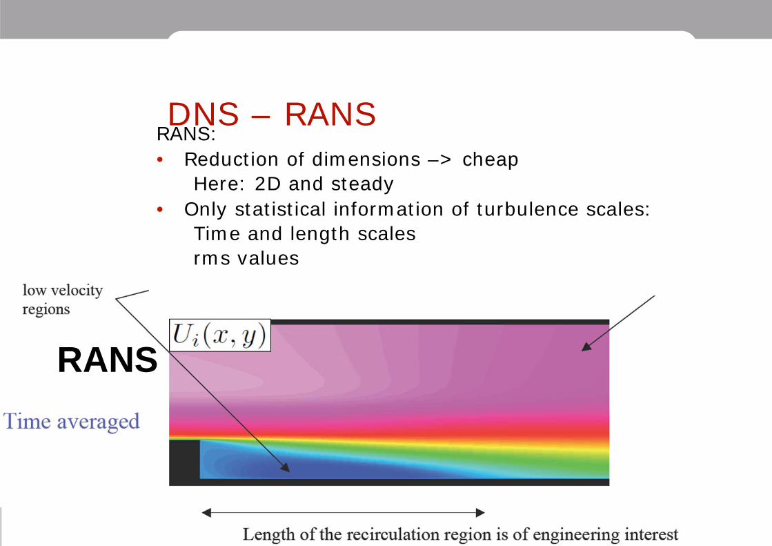
13

RANS:• Reduction of dimensions –> cheap

Here: 2D and steady• Only statistical information of turbulence scales:

Time and length scalesrms values

RANS

DNS – RANS

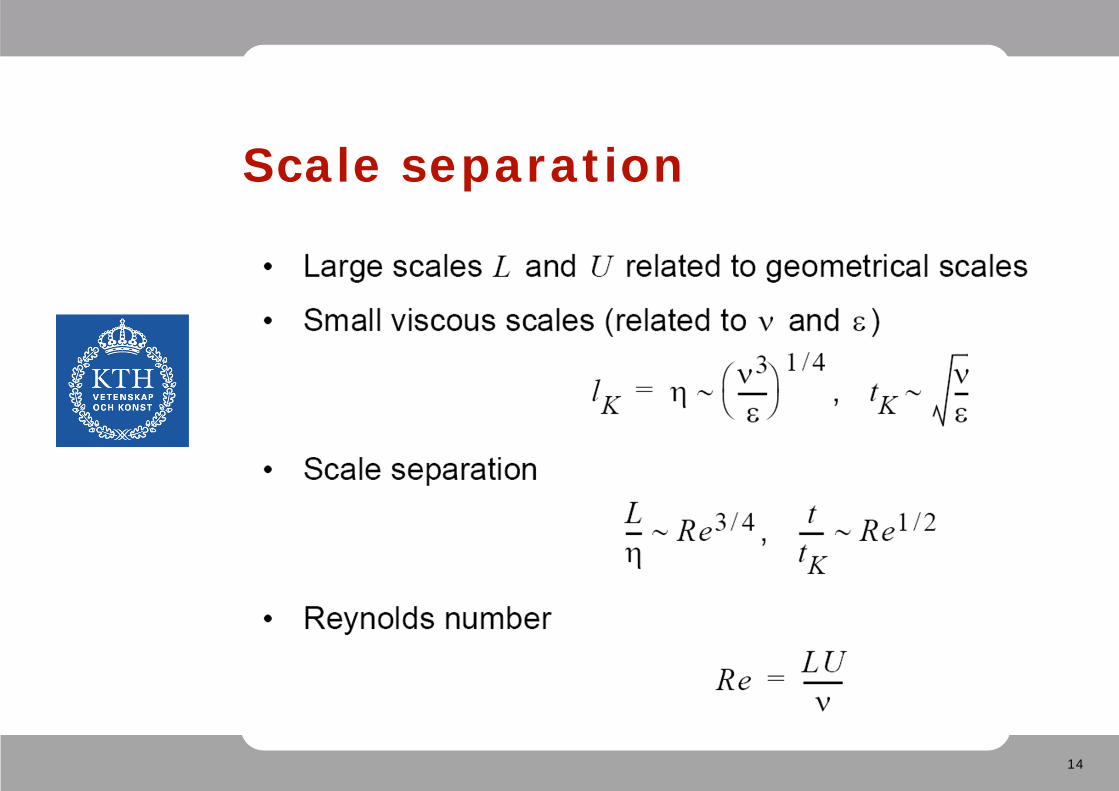
14

Scale separation

15

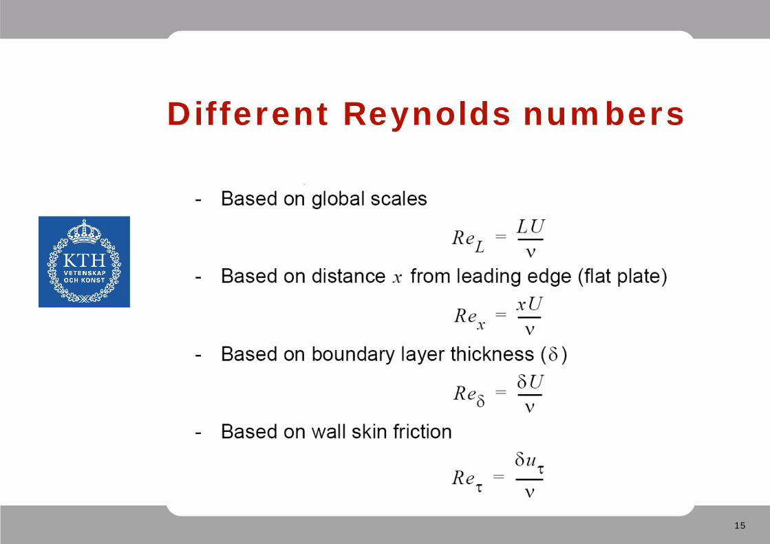
Different Reynolds numbers

16

Viscosity• Kinematic viscosity, • Dynamic viscosity, • Density,

17

Boundary layers (BL)• Thin layers

– Thickness Reynolds number dependent

• Laminar boundary layers– Thickness related to wall skin friction

• Turbulent boundary layers– Inner and outer scales separated– Scale separation Reynolds number dependent

• Figures (Wing+bl – bl – near-wall)

18

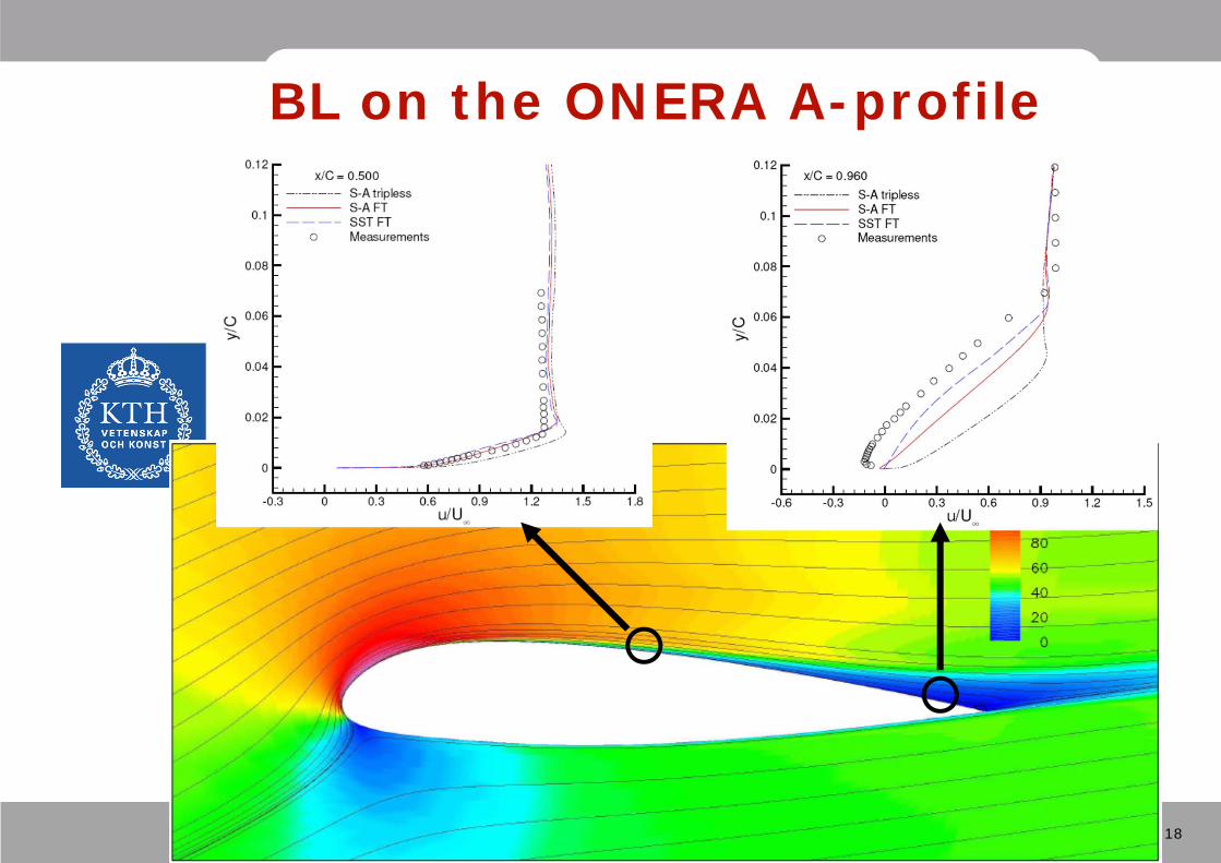
BL on the ONERA A-profile

19

Approximation of BLs• Slip wall boundary condition

– Boundary layer completely neglected– Euler (non-viscous) computations possible– Slip BC can also be applied to viscous & turbulent CFD

• No slip boundary condition– Boundary layer completely resolved (y+=1)– Extreme resolution needed (y=1-100m)– 40-80 grid points within the boundary layer

• Log-law boundary condition (turbulence)– First grid point within log layer (y+>20 AND y<0.1)– 10-20 grid points within the boundary layer– Warning: standard log-law BCs inconsistent with too small

grid size. READ SOLVER DOCUMENTATION !!!

20

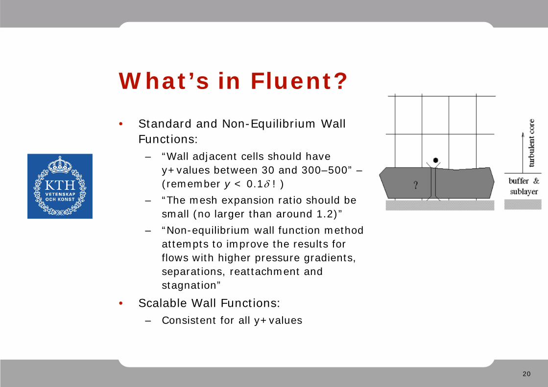
What’s in Fluent?• Standard and Non-Equilibrium Wall

Functions:– “Wall adjacent cells should have

y+values between 30 and 300–500” –(remember y < 0.1 ! )

– “The mesh expansion ratio should be small (no larger than around 1.2)”

– “Non-equilibrium wall function method attempts to improve the results for flows with higher pressure gradients, separations, reattachment and stagnation”

• Scalable Wall Functions:– Consistent for all y+values

21

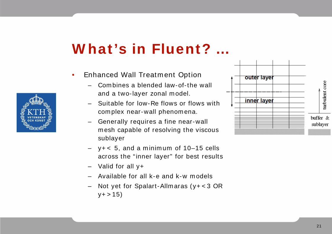
What’s in Fluent? …• Enhanced Wall Treatment Option

– Combines a blended law-of-the wall and a two-layer zonal model.

– Suitable for low-Re flows or flows with complex near-wall phenomena.

– Generally requires a fine near-wall mesh capable of resolving the viscous sublayer

– y+< 5, and a minimum of 10–15 cells across the “inner layer” for best results

– Valid for all y+– Available for all k-e and k-w models– Not yet for Spalart-Allmaras (y+<3 OR

y+>15)

22

Recommendations for Fluent

• For K- models– use Enhanced Wall Treatment: EWT-

• If wall functions are favored with K- models– use scalable wall functions

• For K- models– use the default: EWT-

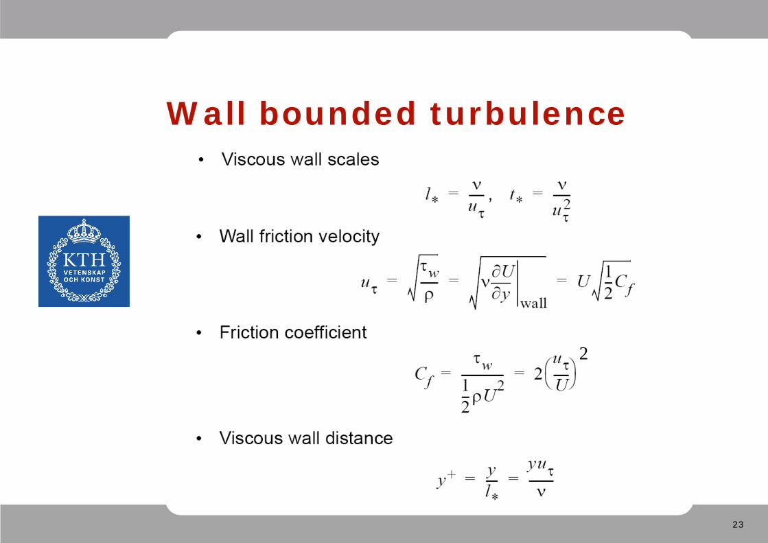
23

Wall bounded turbulence

2

24

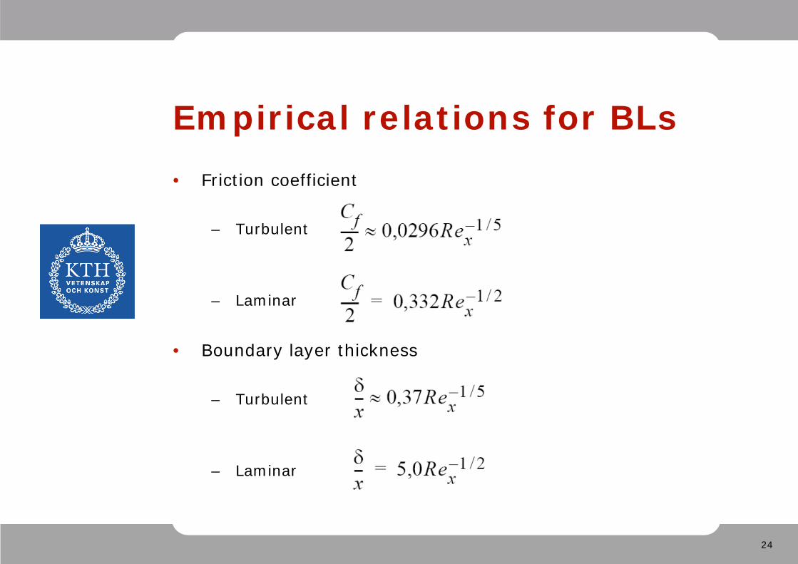
Empirical relations for BLs• Friction coefficient

– Turbulent

– Laminar

• Boundary layer thickness

– Turbulent

– Laminar

25

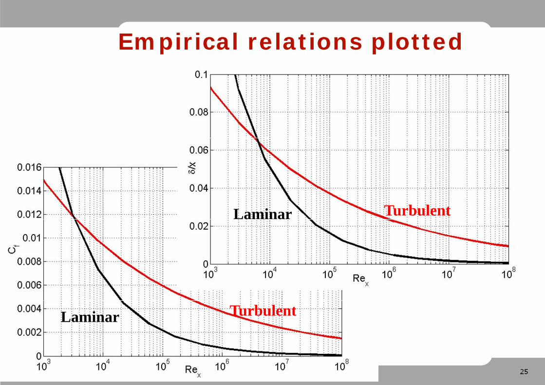
Empirical relations plotted

Laminar Turbulent

Laminar Turbulent

26

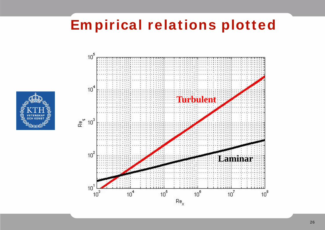
Empirical relations plotted

Laminar

Turbulent

27

Turbulence modelling

28

Reynolds stresses• Not “small”• Significant effects on the flow• Needs to be modelled in terms of mean flow quantities• Reduces the problem to steady (or slowly varying)• 2D assumptions possible

• Equation can be derived from Navier-Stokes equations• Need modelling

29

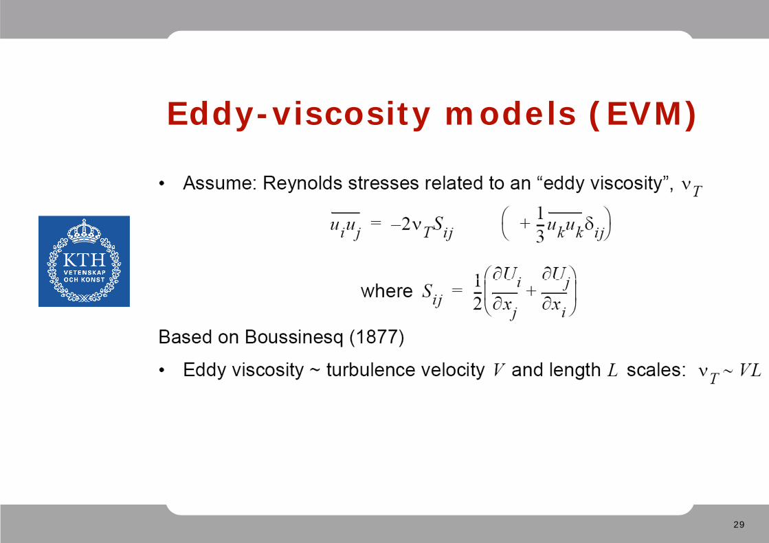
Eddy-viscosity models (EVM)

30

One-equation models• One transport equation for K (turbulent kinetic energy) or T.• Additional information from global conditions (typically wall

distance)• Works well for attached boundary layers• Not very general, but more than algebraic models

• Example: Spalart-Allmaras (1992)– reasonable and robust model for external aerodynamics– Boeing’s ”standard model”

31

Two-equation models• Two transport equations for the turbulence scales (K– or K–)• Completely determined in terms of local quantities (except near-

wall corrections which may be dependent on wall distance)• Works well for attached boundary layers• Somewhat more general than zero-, one-equation models• Model transport equations loosely connected to the exact equations.

• Examples:– Standard K– model (Launder & Spalding 1974)– Wilcox K– (1988, ...) models– Menter (1994) SST K– model (performing reasonable well also in

separated flows)Airbus’ ”standard model”

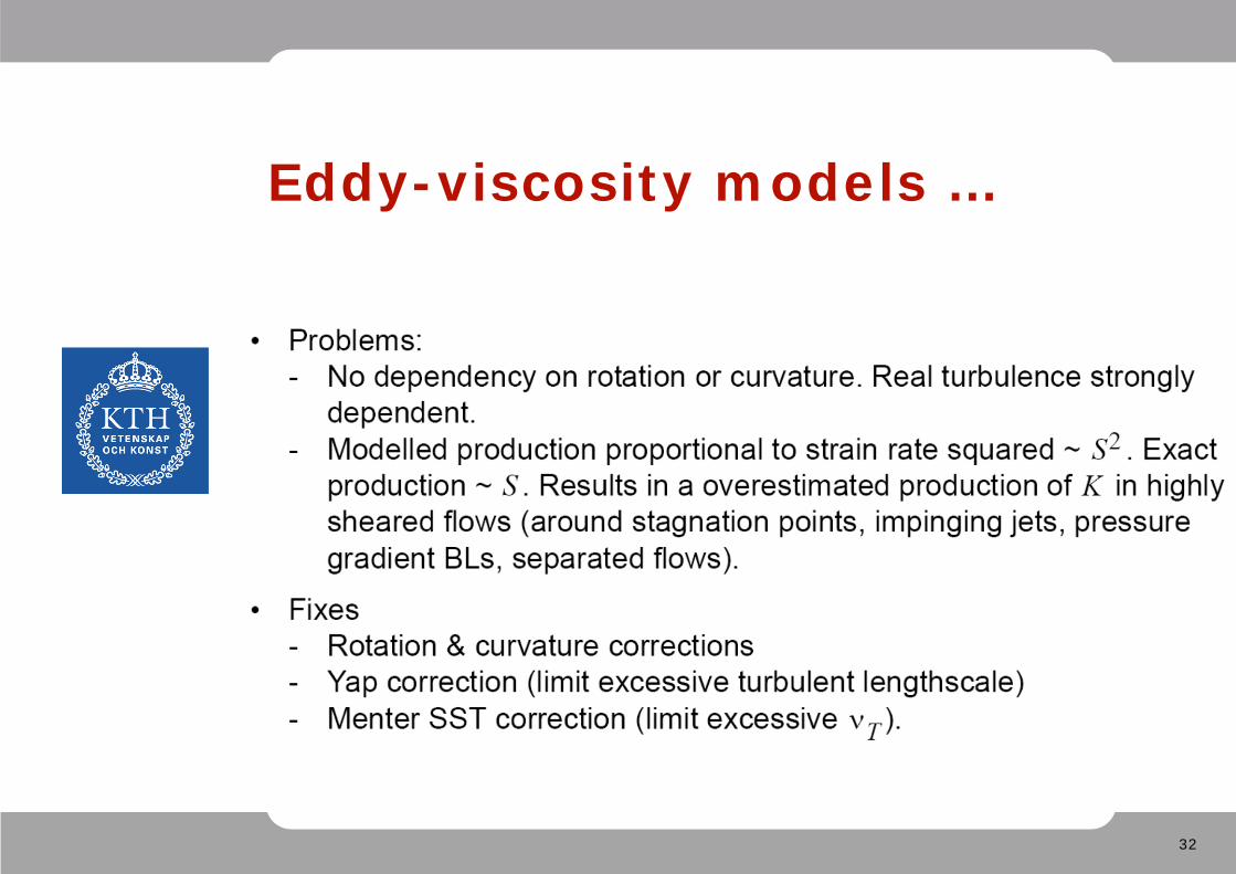
32

Eddy-viscosity models …

33

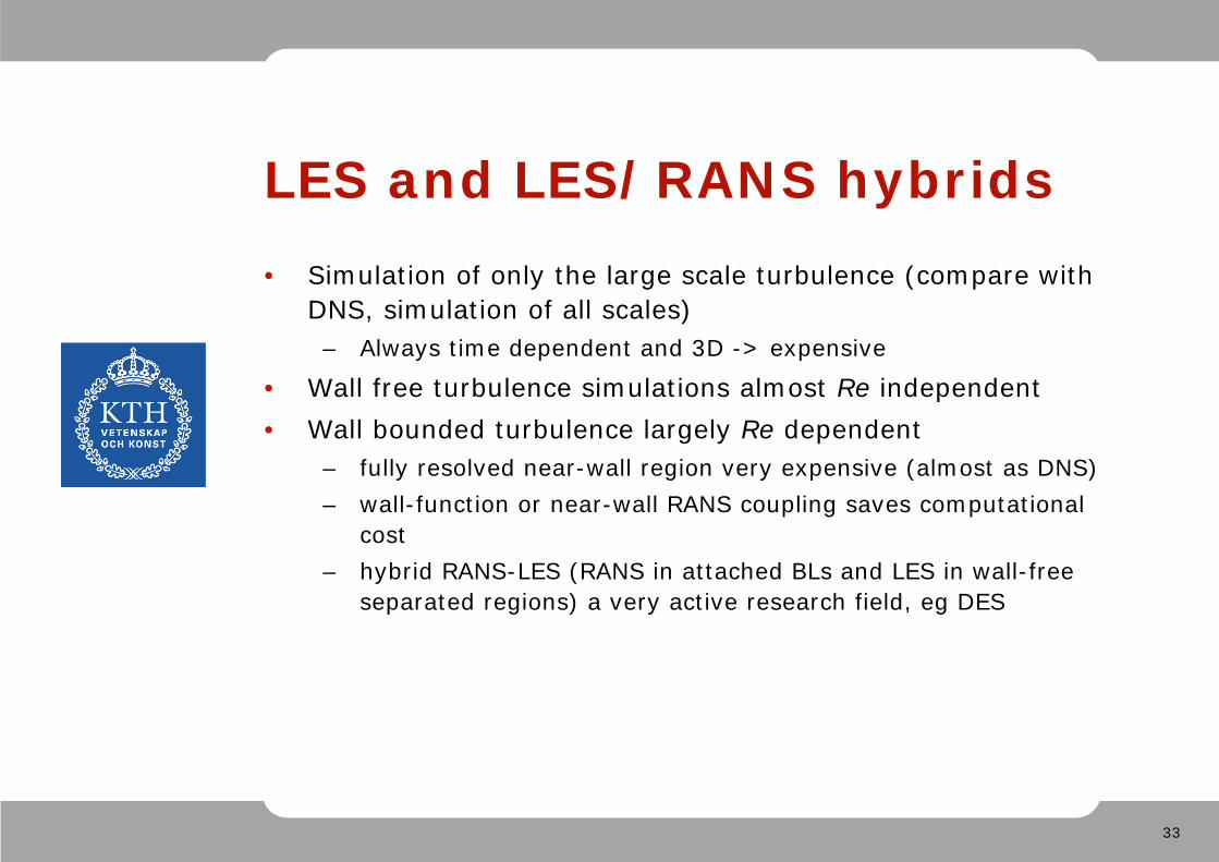
LES and LES/RANS hybrids• Simulation of only the large scale turbulence (compare with

DNS, simulation of all scales)– Always time dependent and 3D -> expensive

• Wall free turbulence simulations almost Re independent• Wall bounded turbulence largely Re dependent

– fully resolved near-wall region very expensive (almost as DNS)– wall-function or near-wall RANS coupling saves computational

cost– hybrid RANS-LES (RANS in attached BLs and LES in wall-free

separated regions) a very active research field, eg DES

34

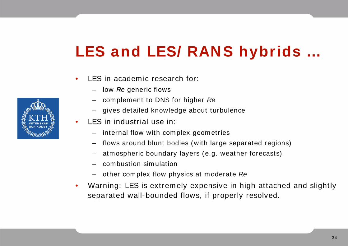
LES and LES/RANS hybrids …• LES in academic research for:

– low Re generic flows– complement to DNS for higher Re– gives detailed knowledge about turbulence

• LES in industrial use in:– internal flow with complex geometries– flows around blunt bodies (with large separated regions)– atmospheric boundary layers (e.g. weather forecasts)– combustion simulation– other complex flow physics at moderate Re

• Warning: LES is extremely expensive in high attached and slightly separated wall-bounded flows, if properly resolved.

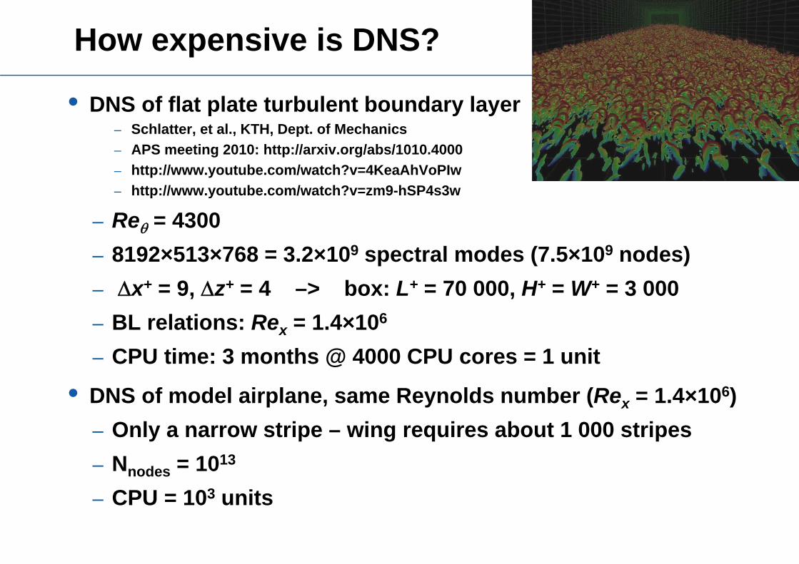
How expensive is DNS?

• DNS of flat plate turbulent boundary layer– Schlatter, et al., KTH, Dept. of Mechanics– APS meeting 2010: http://arxiv.org/abs/1010.4000– http://www.youtube.com/watch?v=4KeaAhVoPIw– http://www.youtube.com/watch?v=zm9-hSP4s3w

– Re = 4300– 8192×513×768 = 3.2×109 spectral modes (7.5×109 nodes)– x+ = 9, z+ = 4 –> box: L+ = 70 000, H+ = W+ = 3 000– BL relations: Rex = 1.4×106

– CPU time: 3 months @ 4000 CPU cores = 1 unit

• DNS of model airplane, same Reynolds number (Rex = 1.4×106) – Only a narrow stripe – wing requires about 1 000 stripes– Nnodes = 1013

– CPU = 103 units

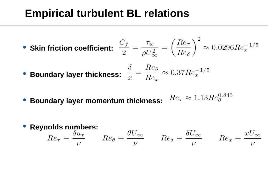
Empirical turbulent BL relations

• Skin friction coefficient:

• Boundary layer thickness:

• Boundary layer momentum thickness:

• Reynolds numbers:

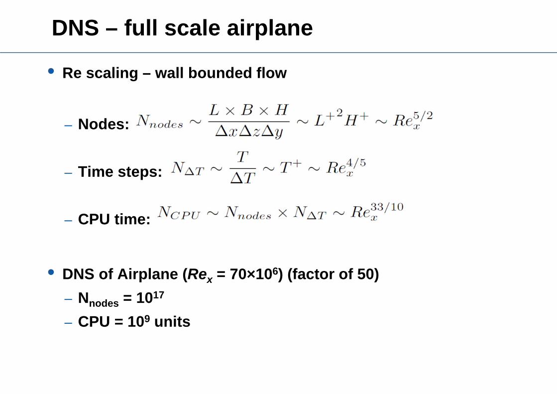
DNS – full scale airplane

• Re scaling – wall bounded flow

– Nodes:

– Time steps:

– CPU time:

• DNS of Airplane (Rex = 70×106) (factor of 50)– Nnodes = 1017

– CPU = 109 units

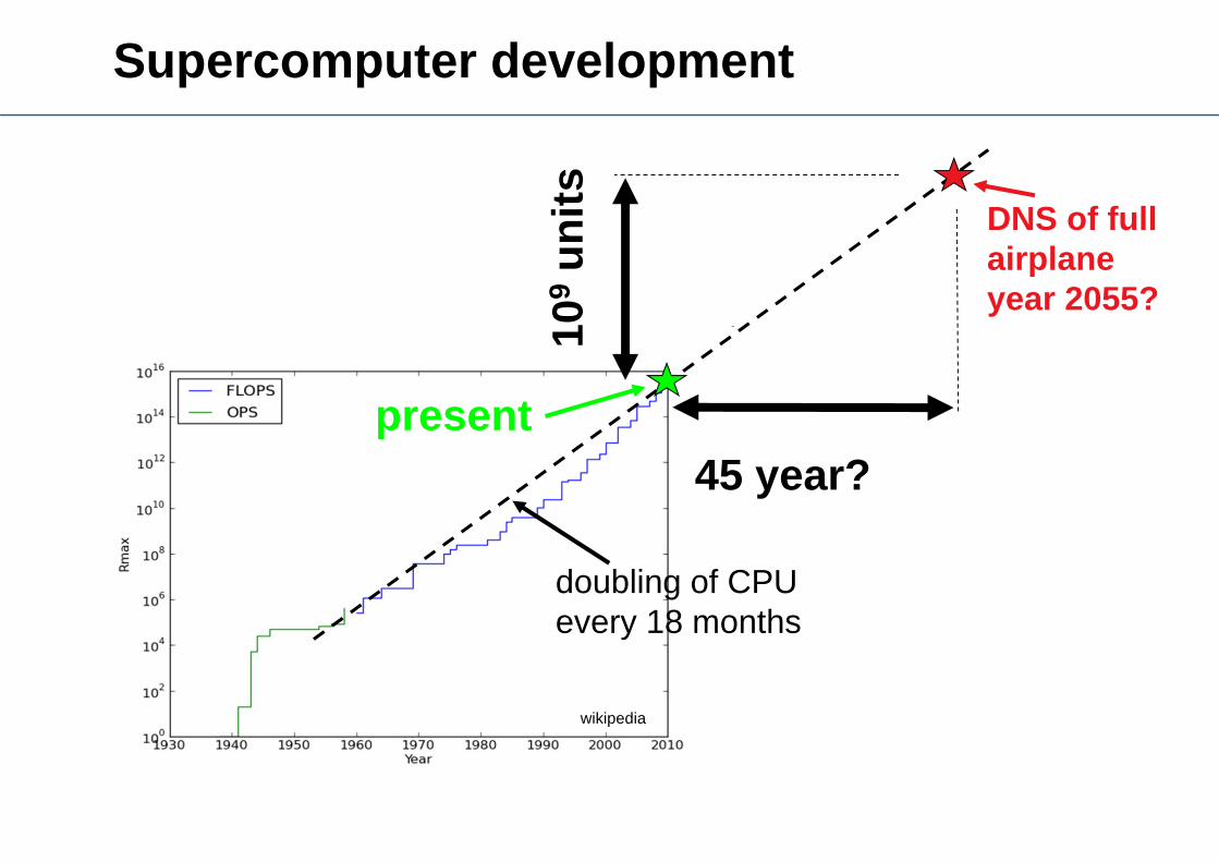
Supercomputer development

wikipedia

present

doubling of CPUevery 18 months

45 year?

109

units DNS of full

airplaneyear 2055?

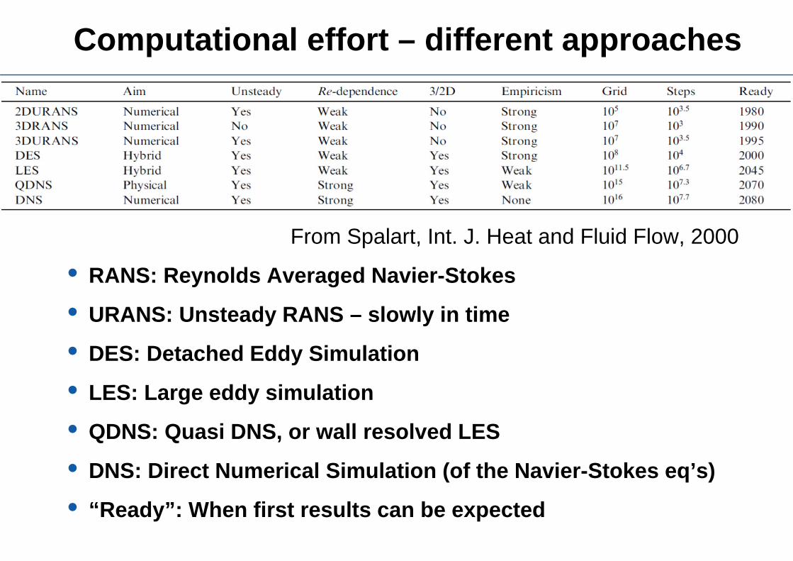
Computational effort – different approaches

From Spalart, Int. J. Heat and Fluid Flow, 2000

• RANS: Reynolds Averaged Navier-Stokes

• URANS: Unsteady RANS – slowly in time

• DES: Detached Eddy Simulation

• LES: Large eddy simulation

• QDNS: Quasi DNS, or wall resolved LES

• DNS: Direct Numerical Simulation (of the Navier-Stokes eq’s)

• “Ready”: When first results can be expected