Embed Size (px)
Citation preview
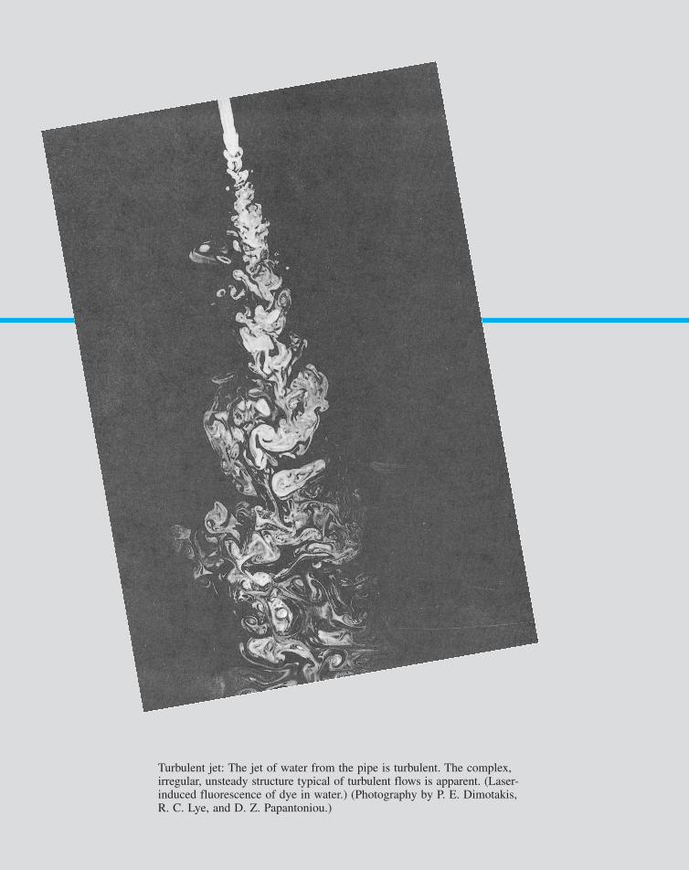
Turbulent jet: The jet of water from the pipe is turbulent. The complex,irregular, unsteady structure typical of turbulent flows is apparent. (Laser-induced fluorescence of dye in water.) (Photography by P. E. Dimotakis,R. C. Lye, and D. Z. Papantoniou.)
7708d_c08_442-531 7/23/01 2:38 PM Page 442
In the previous chapters we have considered a variety of topics concerning the motion offluids. The basic governing principles concerning mass, momentum, and energy were de-veloped and applied, in conjunction with rather severe assumptions, to numerous flow situ-ations. In this chapter we will apply the basic principles to a specific, important topic—theflow of viscous, incompressible fluids in pipes and ducts.
The transport of a fluid 1liquid or gas2 in a closed conduit 1commonly called a pipe ifit is of round cross section or a duct if it is not round2 is extremely important in our dailyoperations. A brief consideration of the world around us will indicate that there is a wide va-riety of applications of pipe flow. Such applications range from the large, man-made Alaskanpipeline that carries crude oil almost 800 miles across Alaska, to the more complex 1and cer-tainly not less useful2 natural systems of “pipes” that carry blood throughout our body andair into and out of our lungs. Other examples include the water pipes in our homes and thedistribution system that delivers the water from the city well to the house. Numerous hosesand pipes carry hydraulic fluid or other fluids to various components of vehicles and ma-chines. The air quality within our buildings is maintained at comfortable levels by the dis-tribution of conditioned 1heated, cooled, humidified�dehumidified2 air through a maze ofpipes and ducts. Although all of these systems are different, the fluid-mechanics principlesgoverning the fluid motions are common. The purpose of this chapter is to understand thebasic processes involved in such flows.
Some of the basic components of a typical pipe system are shown in Fig. 8.1. They in-clude the pipes themselves 1perhaps of more than one diameter2, the various fittings used toconnect the individual pipes to form the desired system, the flowrate control devices 1valves2,and the pumps or turbines that add energy to or remove energy from the fluid. Even the mostsimple pipe systems are actually quite complex when they are viewed in terms of rigorousanalytical considerations. We will use an “exact” analysis of the simplest pipe flow topics1such as laminar flow in long, straight, constant diameter pipes2 and dimensional analysisconsiderations combined with experimental results for the other pipe flow topics. Such anapproach is not unusual in fluid mechanics investigations. When “real world” effects areimportant 1such as viscous effects in pipe flows2, it is often difficult or “impossible” to use
443
8Viscous Flow
in Pipes
Pipe flow is veryimportant in ourdaily operations.
7708d_c08_442-531 7/23/01 2:38 PM Page 443
only theoretical methods to obtain the desired results. A judicious combination of experi-mental data with theoretical considerations and dimensional analysis often provides the de-sired results. The flow in pipes discussed in this chapter is an example of such an analysis.
444 � Chapter 8 / Viscous Flow in Pipes
8.1 General Characteristics of Pipe Flow
Before we apply the various governing equations to pipe flow examples, we will discusssome of the basic concepts of pipe flow. With these ground rules established we can thenproceed to formulate and solve various important flow problems.
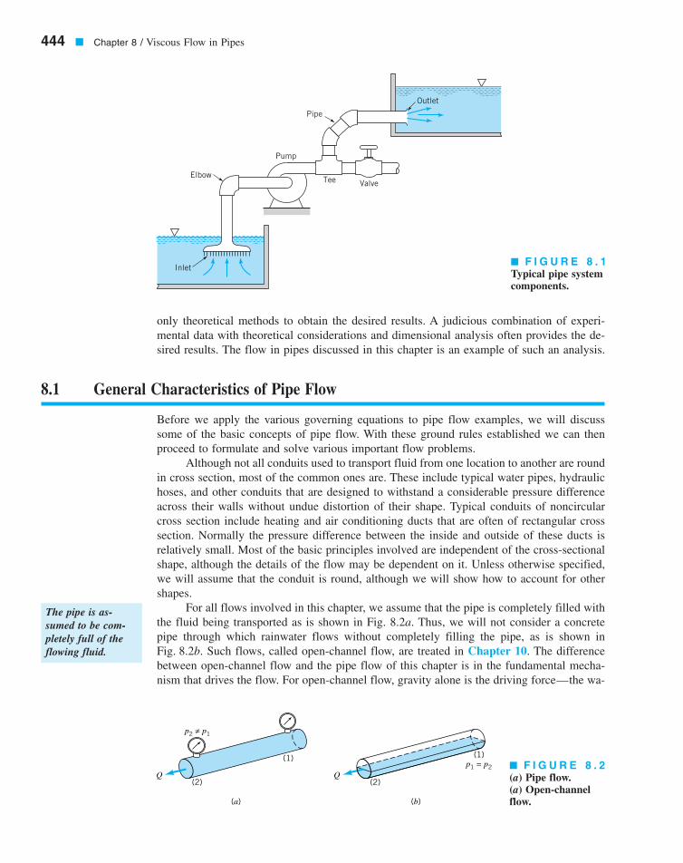
Although not all conduits used to transport fluid from one location to another are roundin cross section, most of the common ones are. These include typical water pipes, hydraulichoses, and other conduits that are designed to withstand a considerable pressure differenceacross their walls without undue distortion of their shape. Typical conduits of noncircularcross section include heating and air conditioning ducts that are often of rectangular crosssection. Normally the pressure difference between the inside and outside of these ducts isrelatively small. Most of the basic principles involved are independent of the cross-sectionalshape, although the details of the flow may be dependent on it. Unless otherwise specified,we will assume that the conduit is round, although we will show how to account for othershapes.
For all flows involved in this chapter, we assume that the pipe is completely filled withthe fluid being transported as is shown in Fig. 8.2a. Thus, we will not consider a concretepipe through which rainwater flows without completely filling the pipe, as is shown inFig. 8.2b. Such flows, called open-channel flow, are treated in Chapter 10. The differencebetween open-channel flow and the pipe flow of this chapter is in the fundamental mecha-nism that drives the flow. For open-channel flow, gravity alone is the driving force—the wa-
Pump
Tee Valve
Outlet
Elbow
Inlet
Pipe
(2)
(a) (b)
(1)
(2)
(1)
Q Q
p2 ≠ p1
p1 = p2
� F I G U R E 8 . 1Typical pipe systemcomponents.
� F I G U R E 8 . 2(a) Pipe flow. (a) Open-channelflow.
The pipe is as-sumed to be com-pletely full of theflowing fluid.
7708d_c08_442-531 7/23/01 2:38 PM Page 444

ter flows down a hill. For pipe flow, gravity may be important 1the pipe need not be hori-zontal2, but the main driving force is likely to be a pressure gradient along the pipe. If thepipe is not full, it is not possible to maintain this pressure difference,
8.1.1 Laminar or Turbulent Flow
The flow of a fluid in a pipe may be laminar flow or it may be turbulent flow. OsborneReynolds 11842–19122, a British scientist and mathematician, was the first to distinguish thedifference between these two classifications of flow by using a simple apparatus as shownin Fig. 8.3a. If water runs through a pipe of diameter D with an average velocity V, the fol-lowing characteristics are observed by injecting neutrally buoyant dye as shown. For “smallenough flowrates” the dye streak 1a streakline2 will remain as a well-defined line as it flowsalong, with only slight blurring due to molecular diffusion of the dye into the surroundingwater. For a somewhat larger “intermediate flowrate” the dye streak fluctuates in time andspace, and intermittent bursts of irregular behavior appear along the streak. On the other hand,for “large enough flowrates” the dye streak almost immediately becomes blurred and spreadsacross the entire pipe in a random fashion. These three characteristics, denoted as laminar,transitional, and turbulent flow, respectively, are illustrated in Fig. 8.3b.
The curves shown in Fig. 8.4 represent the x component of the velocity as a functionof time at a point A in the flow. The random fluctuations of the turbulent flow 1with the as-sociated particle mixing2 are what disperse the dye throughout the pipe and cause the blurredappearance illustrated in Fig. 8.3b. For laminar flow in a pipe there is only one component
p1 � p2.
8.1 General Characteristics of Pipe Flow � 445
Q = VA
D
Dye streak
Dye
Smooth, well-roundedentrance
Pipe
(a) (b)
Laminar
Transitional
Turbulent
Q Ax
uA
t
Laminar
Transitional
Turbulent
� F I G U R E 8 . 3 (a) Experiment to illustrate type of flow. (b) Typical dye streaks.
� F I G U R E 8 . 4Time dependence of fluid velocity at a point.
A flow may be lam-inar, transitional,or turbulent.
V8.1 Laminar/turbulent pipe flow
7708d_c08_442-531 7/23/01 2:38 PM Page 445

of velocity, For turbulent flow the predominant component of velocity is also alongthe pipe, but it is unsteady 1random2 and accompanied by random components normal to thepipe axis, Such motion in a typical flow occurs too fast for our eyes tofollow. Slow motion pictures of the flow can more clearly reveal the irregular, random, tur-bulent nature of the flow.
As was discussed in Chapter 7, we should not label dimensional quantities as being“large” or “small,” such as “small enough flowrates” in the preceding paragraphs. Rather,the appropriate dimensionless quantity should be identified and the “small” or “large” char-acter attached to it. A quantity is “large” or “small” only relative to a reference quantity. Theratio of those quantities results in a dimensionless quantity. For pipe flow the most impor-tant dimensionless parameter is the Reynolds number, Re—the ratio of the inertia to viscouseffects in the flow. Hence, in the previous paragraph the term flowrate should be replacedby Reynolds number, where V is the average velocity in the pipe. That is, theflow in a pipe is laminar, transitional, or turbulent provided the Reynolds number is “smallenough,” “intermediate,” or “large enough.” It is not only the fluid velocity that determinesthe character of the flow—its density, viscosity, and the pipe size are of equal importance.These parameters combine to produce the Reynolds number. The distinction between lami-nar and turbulent pipe flow and its dependence on an appropriate dimensionless quantity wasfirst pointed out by Osborne Reynolds in 1883.
The Reynolds number ranges for which laminar, transitional, or turbulent pipe flowsare obtained cannot be precisely given. The actual transition from laminar to turbulent flowmay take place at various Reynolds numbers, depending on how much the flow is disturbedby vibrations of the pipe, roughness of the entrance region, and the like. For general engi-neering purposes 1i.e., without undue precautions to eliminate such disturbances2, the fol-lowing values are appropriate: The flow in a round pipe is laminar if the Reynolds numberis less than approximately 2100. The flow in a round pipe is turbulent if the Reynolds num-ber is greater than approximately 4000. For Reynolds numbers between these two limits, theflow may switch between laminar and turbulent conditions in an apparently random fashion1transitional flow2.
Re � rVD�m,
V � ui � vj � wk.
V � ui.
446 � Chapter 8 / Viscous Flow in Pipes
EXAMPLE8.1
Water at a temperature of flows through a pipe of diameter 1a2 Determinethe minimum time taken to fill a 12-oz glass with water if the flowin the pipe is to be laminar. 1b2 Determine the maximum time taken to fill the glass if theflow is to be turbulent. Repeat the calculations if the water temperature is
SOLUTION
(a) If the flow in the pipe is to remain laminar, the minimum time to fill the glass will oc-cur if the Reynolds number is the maximum allowed for laminar flow, typically
Thus, where from Table B.1,and at while and
at Thus, the maximum average velocity for lami-nar flow in the pipe is
Similarly, at With of glass and we obtain
V� � QtV� � volume140 °F.V � 0.176 ft�s
� 0.486 ft�s
V �2100m
rD�
210012.73 � 10�5 lb # s�ft2211.94 slugs�ft32 10.73�12 ft2 � 0.486 lb # s�slug
140 °F.m � 0.974 � 10�5 lb # s�ft2r � 1.91 slugs�ft350 °F,m � 2.73 � 10�5 lb # s�ft2slugs�ft3
r � 1.94V � 2100 m�rD,Re � rVD�m � 2100.
140 °F.
1volume � 0.0125 ft32D � 0.73 in.50 °F
Pipe flow character-istics are dependenton the value of theReynolds number.
7708d_c08_442-531 7/23/01 2:38 PM Page 446

8.1.2 Entrance Region and Fully Developed Flow
Any fluid flowing in a pipe had to enter the pipe at some location. The region of flow nearwhere the fluid enters the pipe is termed the entrance region and is illustrated in Fig. 8.5. Itmay be the first few feet of a pipe connected to a tank or the initial portion of a long run ofa hot air duct coming from a furnace.
As is shown in Fig. 8.5, the fluid typically enters the pipe with a nearly uniform ve-locity profile at section 112. As the fluid moves through the pipe, viscous effects cause it tostick to the pipe wall 1the no-slip boundary condition2. This is true whether the fluid is rela-tively inviscid air or a very viscous oil. Thus, a boundary layer in which viscous effects areimportant is produced along the pipe wall such that the initial velocity profile changes withdistance along the pipe, x, until the fluid reaches the end of the entrance length, section 122,beyond which the velocity profile does not vary with x. The boundary layer has grown in
8.1 General Characteristics of Pipe Flow � 447
Inviscid coreBoundary layer
Entrance regionflow
Fully developedflow
D
xr
(2)(1)
�e
(3)
(4)(5)(6)
x6 – x5
Fully developedflow
x5 – x4
Developingflow
� F I G U R E 8 . 5 Entrance region, developing flow, and fully developed flow in a pipe system.
(Ans)
Similarly, at To maintain laminar flow, the less viscous hot water re-quires a lower flowrate than the cold water.
(b) If the flow in the pipe is to be turbulent, the maximum time to fill the glass will occurif the Reynolds number is the minimum allowed for turbulent flow, Thus,
and at while andat
Note that because water is “not very viscous,” the velocity must be “fairly small” tomaintain laminar flow. In general, turbulent flows are encountered more often than laminarflows because of the relatively small viscosity of most common fluids 1water, gasoline, air2.If the flowing fluid had been honey with a kinematic viscosity times greaterthan that of water, the above velocities would be increased by a factor of 3000 and the timesreduced by the same factor. As we will see in the following sections, the pressure needed toforce a very viscous fluid through a pipe at such a high velocity may be unreasonably large.
1n � m�r2 3000
140 °F.t � 12.8 sV � 0.335 ft�s50 °F,t � 4.65 sV � 4000m�rD � 0.925 ft�s
Re � 4000.
140 °F.t � 24.4 s
� 8.85 s at T � 50 °F
t �V�
Q�
V�
1p�42D2V�
410.0125 ft321p 30.73�12 4 2ft22 10.486 ft�s2
Flow in the en-trance region of a pipe is quite complex.
7708d_c08_442-531 7/23/01 2:38 PM Page 447

thickness to completely fill the pipe. Viscous effects are of considerable importance withinthe boundary layer. For fluid outside the boundary layer [within the inviscid core surround-ing the centerline from 112 to 122], viscous effects are negligible.
The shape of the velocity profile in the pipe depends on whether the flow is laminaror turbulent, as does the length of the entrance region, As with many other properties ofpipe flow, the dimensionless entrance length, correlates quite well with the Reynoldsnumber. Typical entrance lengths are given by
(8.1)
and
(8.2)
For very low Reynolds number flows the entrance length can be quite short ifwhereas for large Reynolds number flows it may take a length equal to many pipe
diameters before the end of the entrance region is reached for Formany practical engineering problems, so that
Calculation of the velocity profile and pressure distribution within the entrance regionis quite complex. However, once the fluid reaches the end of the entrance region, section 122of Fig. 8.5, the flow is simpler to describe because the velocity is a function of only the dis-tance from the pipe centerline, r, and independent of x. This is true until the character of thepipe changes in some way, such as a change in diameter, or the fluid flows through a bend,valve, or some other component at section 132. The flow between 122 and 132 is termed fullydeveloped. Beyond the interruption of the fully developed flow [at section 142], the flow grad-ually begins its return to its fully developed character [section 152] and continues with thisprofile until the next pipe system component is reached [section 162]. In many cases the pipeis long enough so that there is a considerable length of fully developed flow compared withthe developing flow length and In other cases thedistances between one component 1bend, tee, valve, etc.2 of the pipe system and the nextcomponent is so short that fully developed flow is never achieved.
8.1.3 Pressure and Shear Stress
Fully developed steady flow in a constant diameter pipe may be driven by gravity and�orpressure forces. For horizontal pipe flow, gravity has no effect except for a hydrostatic pres-sure variation across the pipe, that is usually negligible. It is the pressure difference,
between one section of the horizontal pipe and another which forces the fluidthrough the pipe. Viscous effects provide the restraining force that exactly balances the pres-sure force, thereby allowing the fluid to flow through the pipe with no acceleration. If vis-cous effects were absent in such flows, the pressure would be constant throughout the pipe,except for the hydrostatic variation.
In non-fully developed flow regions, such as the entrance region of a pipe, the fluidaccelerates or decelerates as it flows 1the velocity profile changes from a uniform profile atthe entrance of the pipe to its fully developed profile at the end of the entrance region2. Thus,in the entrance region there is a balance between pressure, viscous, and inertia 1acceleration2forces. The result is a pressure distribution along the horizontal pipe as shown in Fig. 8.6.The magnitude of the pressure gradient, is larger in the entrance region than in thefully developed region, where it is a constant,
The fact that there is a nonzero pressure gradient along the horizontal pipe is a resultof viscous effects. As is discussed in Chapter 3, if the viscosity were zero, the pressure wouldnot vary with x. The need for the pressure drop can be viewed from two different standpoints.
0p�0x � �¢p�/ 6 0.0p�0x,
¢p � p1 � p2,gD,
1x6 � x52 � 1x5 � x42 4 .3 1x3 � x22 � /e
20D 6 /e 6 30D.104 6 Re 6 105Re � 20002.1/e � 120D
Re � 102,1/e � 0.6D
/e
D� 4.4 1Re21�6 for turbulent flow
/e
D� 0.06 Re for laminar flow
/e�D,/e.
448 � Chapter 8 / Viscous Flow in Pipes
The entrance lengthis a function of theReynolds number.
7708d_c08_442-531 7/23/01 2:38 PM Page 448

In terms of a force balance, the pressure force is needed to overcome the viscous forces gen-erated. In terms of an energy balance, the work done by the pressure force is needed to over-come the viscous dissipation of energy throughout the fluid. If the pipe is not horizontal, thepressure gradient along it is due in part to the component of weight in that direction. As isdiscussed in Section 8.2.1, this contribution due to the weight either enhances or retards theflow, depending on whether the flow is downhill or uphill.
The nature of the pipe flow is strongly dependent on whether the flow is laminar orturbulent. This is a direct consequence of the differences in the nature of the shear stress inlaminar and turbulent flows. As is discussed in some detail in Section 8.3.3, the shear stressin laminar flow is a direct result of momentum transfer among the randomly moving mole-cules 1a microscopic phenomenon2. The shear stress in turbulent flow is largely a result ofmomentum transfer among the randomly moving, finite-sized bundles of fluid particles 1amacroscopic phenomenon2. The net result is that the physical properties of the shear stressare quite different for laminar flow than for turbulent flow.
8.2 Fully Developed Laminar Flow � 449
8.2 Fully Developed Laminar Flow
As is indicated in the previous section, the flow in long, straight, constant diameter sectionsof a pipe becomes fully developed. That is, the velocity profile is the same at any cross sec-tion of the pipe. Although this is true whether the flow is laminar or turbulent, the details ofthe velocity profile 1and other flow properties2 are quite different for these two types of flow.As will be seen in the remainder of this chapter, knowledge of the velocity profile can leaddirectly to other useful information such as pressure drop, head loss, flowrate, and the like.Thus, we begin by developing the equation for the velocity profile in fully developed lami-nar flow. If the flow is not fully developed, a theoretical analysis becomes much more com-plex and is outside the scope of this text. If the flow is turbulent, a rigorous theoretical analy-sis is as yet not possible.
Although most flows are turbulent rather than laminar, and many pipes are not longenough to allow the attainment of fully developed flow, a theoretical treatment and full un-derstanding of fully developed laminar flow is of considerable importance. First, it repre-sents one of the few theoretical viscous analyses that can be carried out “exactly” 1within theframework of quite general assumptions2 without using other ad hoc assumptions or ap-proximations. An understanding of the method of analysis and the results obtained providesa foundation from which to carry out more complicated analyses. Second, there are manypractical situations involving the use of fully developed laminar pipe flow.
Entrancepressure
drop
Entrance flow Fully developedflow: p/ x = constant∂∂
∆p
x3 – x2 = �
x2 = �ex1 = 0
p
x3 x
� F I G U R E 8 . 6 Pressure distribution along a horizontal pipe.
Laminar flow char-acteristics are dif-ferent than thosefor turbulent flow.
7708d_c08_442-531 7/23/01 2:38 PM Page 449
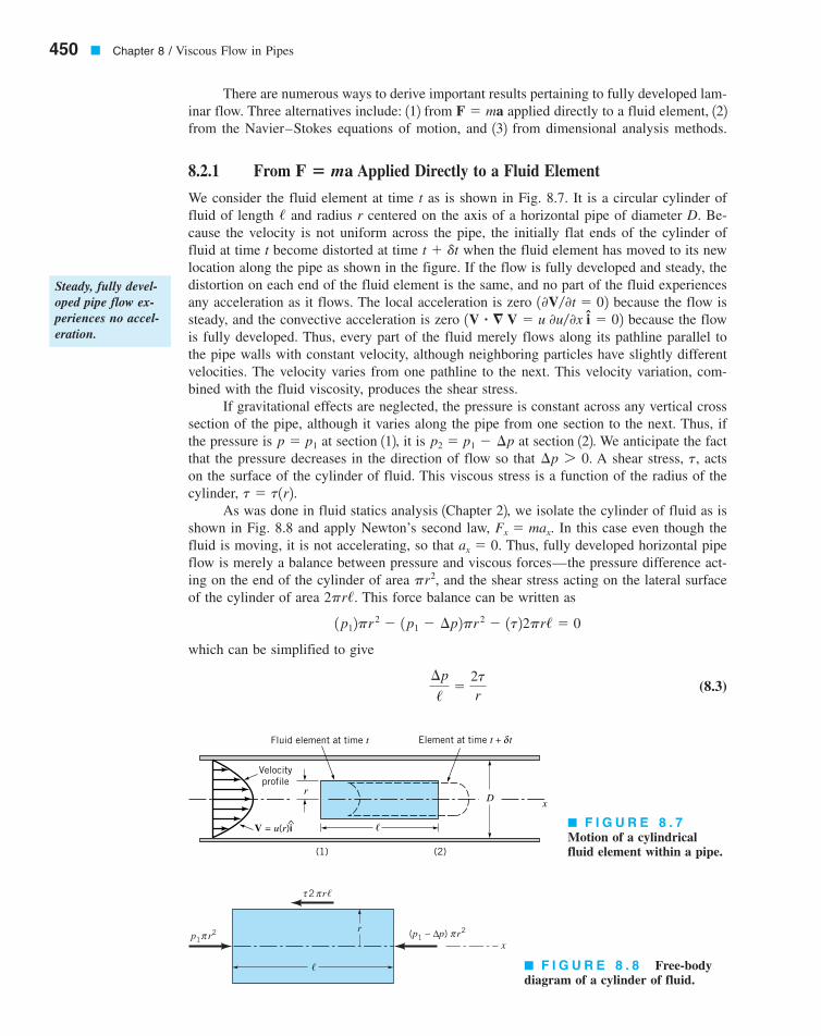
There are numerous ways to derive important results pertaining to fully developed lam-inar flow. Three alternatives include: 112 from applied directly to a fluid element, 122from the Navier–Stokes equations of motion, and 132 from dimensional analysis methods.
8.2.1 From Applied Directly to a Fluid Element
We consider the fluid element at time t as is shown in Fig. 8.7. It is a circular cylinder offluid of length and radius r centered on the axis of a horizontal pipe of diameter D. Be-cause the velocity is not uniform across the pipe, the initially flat ends of the cylinder offluid at time t become distorted at time when the fluid element has moved to its newlocation along the pipe as shown in the figure. If the flow is fully developed and steady, thedistortion on each end of the fluid element is the same, and no part of the fluid experiencesany acceleration as it flows. The local acceleration is zero because the flow issteady, and the convective acceleration is zero because the flowis fully developed. Thus, every part of the fluid merely flows along its pathline parallel tothe pipe walls with constant velocity, although neighboring particles have slightly differentvelocities. The velocity varies from one pathline to the next. This velocity variation, com-bined with the fluid viscosity, produces the shear stress.
If gravitational effects are neglected, the pressure is constant across any vertical crosssection of the pipe, although it varies along the pipe from one section to the next. Thus, ifthe pressure is at section 112, it is at section 122. We anticipate the factthat the pressure decreases in the direction of flow so that A shear stress, actson the surface of the cylinder of fluid. This viscous stress is a function of the radius of thecylinder,
As was done in fluid statics analysis 1Chapter 22, we isolate the cylinder of fluid as isshown in Fig. 8.8 and apply Newton’s second law, In this case even though thefluid is moving, it is not accelerating, so that Thus, fully developed horizontal pipeflow is merely a balance between pressure and viscous forces—the pressure difference act-ing on the end of the cylinder of area and the shear stress acting on the lateral surfaceof the cylinder of area This force balance can be written as
which can be simplified to give
(8.3)¢p
/�
2tr
1p12pr 2 � 1p1 � ¢p2pr 2 � 1t22pr/ � 0
2pr/.pr2,
ax � 0.Fx � max.
t � t1r2.t,¢p 7 0.
p2 � p1 � ¢pp � p1
1V � � V � u 0u�0x i � 0210V�0t � 02
t � dt
/
F � ma
F � ma
450 � Chapter 8 / Viscous Flow in Pipes
(1) (2)
D
Velocityprofile
V = u(r)i
r
Fluid element at time t Element at time t + tδ
x
�^
2 r�τ π
(p1 – ∆p) r2πx
r
�
p1 r2π
� F I G U R E 8 . 7Motion of a cylindricalfluid element within a pipe.
� F I G U R E 8 . 8 Free-bodydiagram of a cylinder of fluid.
Steady, fully devel-oped pipe flow ex-periences no accel-eration.
7708d_c08_442-531 7/23/01 2:38 PM Page 450
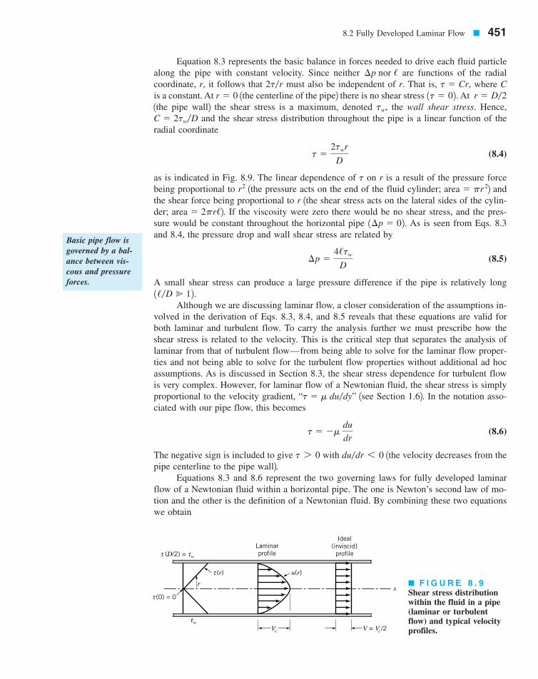
Equation 8.3 represents the basic balance in forces needed to drive each fluid particlealong the pipe with constant velocity. Since neither are functions of the radialcoordinate, r, it follows that must also be independent of r. That is, where Cis a constant. At 1the centerline of the pipe2 there is no shear stress At 1the pipe wall2 the shear stress is a maximum, denoted the wall shear stress. Hence,
and the shear stress distribution throughout the pipe is a linear function of theradial coordinate
(8.4)
as is indicated in Fig. 8.9. The linear dependence of on r is a result of the pressure forcebeing proportional to 1the pressure acts on the end of the fluid cylinder; 2 andthe shear force being proportional to r 1the shear stress acts on the lateral sides of the cylin-der; area 2. If the viscosity were zero there would be no shear stress, and the pres-sure would be constant throughout the horizontal pipe As is seen from Eqs. 8.3and 8.4, the pressure drop and wall shear stress are related by
(8.5)
A small shear stress can produce a large pressure difference if the pipe is relatively long
Although we are discussing laminar flow, a closer consideration of the assumptions in-volved in the derivation of Eqs. 8.3, 8.4, and 8.5 reveals that these equations are valid forboth laminar and turbulent flow. To carry the analysis further we must prescribe how theshear stress is related to the velocity. This is the critical step that separates the analysis oflaminar from that of turbulent flow—from being able to solve for the laminar flow proper-ties and not being able to solve for the turbulent flow properties without additional ad hocassumptions. As is discussed in Section 8.3, the shear stress dependence for turbulent flowis very complex. However, for laminar flow of a Newtonian fluid, the shear stress is simplyproportional to the velocity gradient, 1see Section 1.62. In the notation asso-ciated with our pipe flow, this becomes
(8.6)
The negative sign is included to give with 1the velocity decreases from thepipe centerline to the pipe wall2.
Equations 8.3 and 8.6 represent the two governing laws for fully developed laminarflow of a Newtonian fluid within a horizontal pipe. The one is Newton’s second law of mo-tion and the other is the definition of a Newtonian fluid. By combining these two equationswe obtain
du�dr 6 0t 7 0
t � �m du
dr
“t � m du�dy”
1/�D � 12.
¢p �4/tw
D
1¢p � 02.� 2pr/
area � pr 2r2t
t �2twr
D
C � 2tw�Dtw,
r � D�21t � 02.r � 0t � Cr,2t�r
¢p nor /
8.2 Fully Developed Laminar Flow � 451
τVc
(r)τ
r
(0) = 0τ
(D/2) = w τ τLaminarprofile
u(r)
Ideal(inviscid)
profile
x
V = Vc/2w
� F I G U R E 8 . 9Shear stress distributionwithin the fluid in a pipe(laminar or turbulentflow) and typical velocityprofiles.
Basic pipe flow isgoverned by a bal-ance between vis-cous and pressureforces.
7708d_c08_442-531 7/23/01 2:38 PM Page 451

which can be integrated to give the velocity profile as follows:
or
where is a constant. Because the fluid is viscous it sticks to the pipe wall so that at Thus, Hence, the velocity profile can be written as
(8.7)
where is the centerline velocity. An alternative expression can be writ-ten by using the relationship between the wall shear stress and the pressure gradient 1Eqs. 8.5and 8.72 to give
where is the pipe radius.This velocity profile, plotted in Fig. 8.9, is parabolic in the radial coordinate, r, has a
maximum velocity, at the pipe centerline, and a minimum velocity 1zero2 at the pipe wall.The volume flowrate through the pipe can be obtained by integrating the velocity profileacross the pipe. Since the flow is axisymmetric about the centerline, the velocity is constanton small area elements consisting of rings of radius r and thickness dr. Thus,
or
By definition, the average velocity is the flowrate divided by the cross-sectional area,so that for this flow
(8.8)
and
(8.9)
As is indicated in Eq. 8.8, the average velocity is one-half of the maximum velocity. In gen-eral, for velocity profiles of other shapes 1such as for turbulent pipe flow2, the average velocityis not merely the average of the maximum and minimum 102 velocities as it is for thelaminar parabolic profile. The two velocity profiles indicated in Fig. 8.9 provide the same
1Vc2
Q �pD4 ¢p
128m/
V �pR2Vc
2pR2 �Vc
2�
¢pD2
32m/
V � Q�A � Q�pR2,
Q �pR2Vc
2
Q � � u dA � �r�R
r�0 u1r22pr dr � 2p Vc�
R
0 c1 � a r
Rb2 d r dr
Vc ,
R � D�2
u1r2 �twD
4m c1 � a r
Rb2 d
Vc � ¢pD2� 116m/2u1r2 � a¢pD2
16m/b c1 � a2r
Db2 d � Vc c1 � a2r
Db2 d
C1 � 1¢p�16m/2D2.r � D�2.u � 0C1
u � �a ¢p
4m/b r 2 � C1
� du � �¢p
2m/ � r dr
du
dr� �a ¢p
2m/b r
452 � Chapter 8 / Viscous Flow in Pipes
Under certain re-strictions the veloc-ity profile in a pipeis parabolic.
7708d_c08_442-531 7/23/01 2:38 PM Page 452
flowrate—one is the fictitious ideal profile; the other is the actual laminar flowprofile.
The above results confirm the following properties of laminar pipe flow. For a hori-zontal pipe the flowrate is 1a2 directly proportional to the pressure drop, 1b2 inversely pro-portional to the viscosity, 1c2 inversely proportional to the pipe length, and 1d2 proportionalto the pipe diameter to the fourth power. With all other parameters fixed, an increase in di-ameter by a factor of 2 will increase the flowrate by a factor of 16—the flowrate is verystrongly dependent on pipe size. A 2% error in diameter gives an 8% error in flowrate or so that This flow, the properties of which were first es-tablished experimentally by two independent workers, G. Hagen 11797–18842 in 1839 andJ. Poiseuille 11799–18692 in 1840, is termed Hagen–Poiseuille flow. Equation 8.9 is com-monly referred to as Poiseuille’s law. Recall that all of these results are restricted to laminarflow 1those with Reynolds numbers less than approximately 21002 in a horizontal pipe.
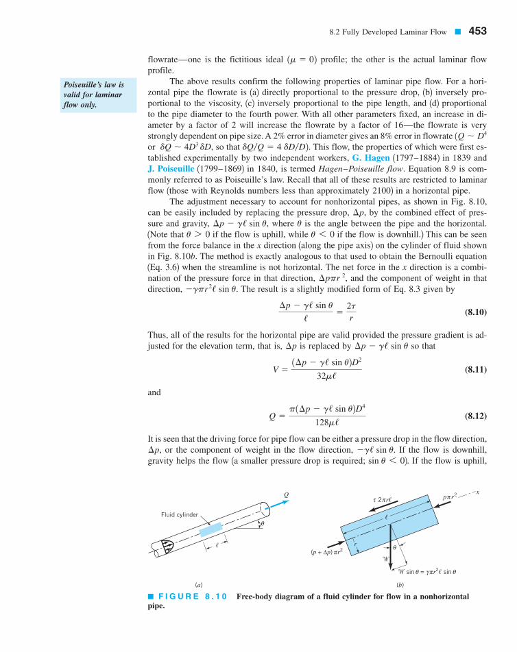
The adjustment necessary to account for nonhorizontal pipes, as shown in Fig. 8.10,can be easily included by replacing the pressure drop, by the combined effect of pres-sure and gravity, , where is the angle between the pipe and the horizontal.1Note that if the flow is uphill, while if the flow is downhill.2 This can be seenfrom the force balance in the x direction 1along the pipe axis2 on the cylinder of fluid shownin Fig. 8.10b. The method is exactly analogous to that used to obtain the Bernoulli equation1Eq. 3.62 when the streamline is not horizontal. The net force in the x direction is a combi-nation of the pressure force in that direction, and the component of weight in thatdirection, The result is a slightly modified form of Eq. 8.3 given by
(8.10)
Thus, all of the results for the horizontal pipe are valid provided the pressure gradient is ad-justed for the elevation term, that is, is replaced by so that
(8.11)
and
(8.12)
It is seen that the driving force for pipe flow can be either a pressure drop in the flow direction,or the component of weight in the flow direction, If the flow is downhill,
gravity helps the flow 1a smaller pressure drop is required; 2. If the flow is uphill,sin u 6 0�g/ sin u.¢p,
Q �p1¢p � g/ sin u2D4
128m/
V �1¢p � g/ sin u2D2
32m/
¢p � g/ sin u¢p
¢p � g/ sin u
/�
2tr
�gpr 2/ sin u.¢ppr 2,
u 6 0u 7 0u¢p � g/ sin u
¢p,
dQ�Q � 4 dD�D2.dQ � 4D3 dD,1Q � D4
1m � 02
8.2 Fully Developed Laminar Flow � 453
�
� sin = r2� sinθ θγπ
πp r2 x
θ(p + ∆p) r2
r
�
2 r�τ
(b)(a)
�
Fluid cylinderθ
Q
π
π
� F I G U R E 8 . 1 0 Free-body diagram of a fluid cylinder for flow in a nonhorizontalpipe.
Poiseuille’s law isvalid for laminarflow only.
7708d_c08_442-531 7/23/01 2:38 PM Page 453

gravity works against the flow 1a larger pressure drop is required; 2. Note that1where is the change in elevation2 is a hydrostatic type pressure term. Ifthere is no flow, as expected for fluid statics.V � 0 and ¢p � g/ sin u � g¢z,
¢zg/ sin u � g¢zsin u 7 0
454 � Chapter 8 / Viscous Flow in Pipes
EXAMPLE8.2
An oil with a viscosity of and density flows in a pipe ofdiameter 1a2What pressure drop, is needed to produce a flowrate of
if the pipe is horizontal with and 1b2 How steep ahill, must the pipe be on if the oil is to flow through the pipe at the same rate as in part1a2, but with 1c2 For the conditions of part 1b2, if what is the pressureat section where x is measured along the pipe?
SOLUTION
(a) If the Reynolds number is less than 2100 the flow is laminar and the equations derivedin this section are valid. Since the average velocity is
the Reynolds number is Hence, the flow is laminar and from Eq. 8.9 with the
pressure drop is
or
(Ans)
(b) If the pipe is on a hill of angle such that Eq. 8.12 gives
(1)
or
Thus, (Ans)This checks with the previous horizontal result as is seen from the fact that a
change in elevation of is equivalentto a pressure change of
which is equivalent to that needed for the horizontal pipe. For the horizontal pipeit is the work done by the pressure forces that overcomes the viscous dissipation. Forthe zero-pressure-drop pipe on the hill, it is the change in potential energy of the fluid“falling” down the hill that is converted to the energy lost by viscous dissipation. Notethat if it is desired to increase the flowrate to with thevalue of given by Eq. 1 is Since the sine of an angle cannot be greaterthan 1, this flow would not be possible. The weight of the fluid would not be largeenough to offset the viscous force generated for the flowrate desired. A larger diame-ter pipe would be needed.
sin u � �1.15.u
p1 � p2,Q � 1.0 � 10�4 m3�s
N�m2,¢p � rg ¢z � 1900 kg�m32 19.81 m�s22 12.31 m2 � 20,400
¢z � / sin u � 110 m2 sin1�13.34°2 � �2.31 m
u � �13.34°.
sin u ��12810.40 N # s�m22 12.0 � 10�5 m3�s2p1900 kg�m32 19.81 m�s22 10.020 m24
sin u � �128mQ
prgD4
¢p � p1 � p2 � 0,u
¢p � 20,400 N�m2 � 20.4 kPa
�12810.40 N # s�m22 110.0 m2 12.0 � 10�5 m3�s2
p10.020 m24
¢p � p1 � p2 �128m/Q
pD4
/ � x2 � x1 � 10 m,6 2100.Re � rVD�m � 2.87m3�s2� 3p10.02022m2�4 4 � 0.0637 m�s,
V � Q�A � 12.0 � 10�5
x3 � 5 m,p1 � 200 kPa,p1 � p2?
u,x2 � 10 m?x1 � 0Q � 2.0 � 10�5 m3�s
p1 � p2,D � 0.020 m.r � 900 kg�m3m � 0.40 N # s�m2
7708d_c08_442-531 7/23/01 2:38 PM Page 454

8.2.2 From the Navier–Stokes Equations
In the previous section we obtained results for fully developed laminar pipe flow by apply-ing Newton’s second law and the assumption of a Newtonian fluid to a specific portion ofthe fluid—a cylinder of fluid centered on the axis of a long, round pipe. When this govern-ing law and assumptions are applied to a general fluid flow 1not restricted to pipe flow2, theresult is the Navier–Stokes equations as discussed in Chapter 6. In Section 6.9.3 these equa-tions were solved for the specific geometry of fully developed laminar flow in a round pipe.The results are the same as those given in Eq. 8.7.
We will not repeat the detailed steps used to obtain the laminar pipe flow from theNavier–Stokes equations 1see Section 6.9.32 but will indicate how the various assumptionsused and steps applied in the derivation correlate with the analysis used in the previoussection.
General motion of an incompressible Newtonian fluid is governed by the continuityequation 1conservation of mass, Eq. 6.312 and the momentum equation 1Eq. 6.1272, which arerewritten here for convenience:
(8.13)
(8.14)
For steady, fully developed flow in a pipe, the velocity contains only an axial component,which is a function of only the radial coordinate For such conditions, the left-hand side of the Eq. 8.14 is zero. This is equivalent to saying that the fluid experiences noacceleration as it flows along. The same constraint was used in the previous section whenconsidering for the fluid cylinder. Thus, with the Navier–Stokes equationsbecome
(8.15)
The flow is governed by a balance of pressure, weight, and viscous forces in the flow di-rection, similar to that shown in Fig. 8.10 and Eq. 8.10. If the flow were not fully developed1as in an entrance region, for example2, it would not be possible to simplify the Navier–Stokesequations to that form given in Eq. 8.15 1the nonlinear term would not be zero2, andthe solution would be very difficult to obtain.
V � �V
�p � rgk � m�2V
� � V � 0
g � �gkF � ma
3V � u1r2 i 4 .
0V0t
� V � �V � ��pr
� g � n�2V
� � V � 0
8.2 Fully Developed Laminar Flow � 455
(c) With the length of the pipe, does not appear in the flowrate equation 1Eq. 12.This is a statement of the fact that for such cases the pressure is constant all alongthe pipe 1provided the pipe lies on a hill of constant slope2. This can be seen by sub-stituting the values of Q and from case 1b2 into Eq. 8.12 and noting that forany For example, if Thus, sothat
(Ans)
Note that if the fluid were gasoline and the Reynolds number would be the flow would probably not be lam-
inar, and a use of Eqs. 8.9 and 8.12 would give incorrect results. Also note from Eq. 1that the kinematic viscosity, is the important viscous parameter. This is a state-ment of the fact that with constant pressure along the pipe, it is the ratio of the viscousforce to the weight force that determines the value of u.1�g � rg21�m2
n � m�r,
Re � 2790,m32, r � 680 kg�1m � 3.1 � 10�4 N # s�m2
p3 � 200 kPa
p1 � p2 � p3/ � x3 � x1 � 5 m.¢p � p1 � p3 � 0/.¢p � 0u
/,p1 � p2
Poiseuille’s law canbe obtained fromthe Navier–Stokesequations.
7708d_c08_442-531 7/23/01 2:38 PM Page 455

Because of the assumption that the continuity equation, Eq. 8.13, is auto-matically satisfied. This conservation of mass condition was also automatically satisfied bythe incompressible flow assumption in the derivation in the previous section. The fluid flowsacross one section of the pipe at the same rate that it flows across any other section 1seeFig. 8.82.
When it is written in terms of polar coordinates 1as was done in Section 6.9.32, thecomponent of Eq. 8.15 along the pipe becomes
(8.16)
Since the flow is fully developed, and the right-hand side is a function of, at most,only r. The left-hand side is a function of, at most, only x. It was shown that this leads tothe condition that the pressure gradient in the x direction is a constant—The same condition was used in the derivation of the previous section 1Eq. 8.32.
It is seen from Eq. 8.16 that the effect of a nonhorizontal pipe enters into the Navier–Stokes equations in the same manner as was discussed in the previous section. The pressuregradient in the flow direction is coupled with the effect of the weight in that direction to pro-duce an effective pressure gradient of
The velocity profile is obtained by integration of Eq. 8.16. Since it is a second-orderequation, two boundary conditions are needed—112 the fluid sticks to the pipe wall 1as wasalso done in Eq. 8.72 and 122 either of the equivalent forms that the velocity remains finitethroughout the flow 1in particular at 2, or because of symmetry, at
In the derivation of the previous section, only one boundary condition 1the no-slipcondition at the wall2 was needed because the equation integrated was a first-order equation.The other condition was automatically built into the analysis becauseof the fact that and at
The results obtained by either applying to a fluid cylinder 1Section 8.2.12 orsolving the Navier–Stokes equations 1Section 6.9.32 are exactly the same. Similarly, the basicassumptions regarding the flow structure are the same. This should not be surprising becausethe two methods are based on the same principle—Newton’s second law. One is restrictedto fully developed laminar pipe flow from the beginning 1the drawing of the free-body dia-gram2, and the other starts with the general governing equations 1the Navier–Stokes equa-tions2 with the appropriate restrictions concerning fully developed laminar flow applied asthe solution process progresses.
8.2.3 From Dimensional Analysis
Although fully developed laminar pipe flow is simple enough to allow the rather straight-forward solutions discussed in the previous two sections, it may be worthwhile to considerthis flow from a dimensional analysis standpoint. Thus, we assume that the pressure drop inthe horizontal pipe, is a function of the average velocity of the fluid in the pipe, V, thelength of the pipe, the pipe diameter, D, and the viscosity of the fluid, We have not in-cluded the density or the specific weight of the fluid as parameters because for such flowsthey are not important parameters. There is neither mass 1density2 times acceleration nor acomponent of weight 1specific weight times volume2 in the flow direction involved. Thus,
There are five variables that can be described in terms of three reference dimensions 1M, L,T 2. According to the results of dimensional analysis 1Chapter 72, this flow can be describedin terms of dimensionless groups. One such representation isk � r � 5 � 3 � 2
¢p � F1V, /, D, m2
m./,¢p,
F � mar � 0.t � 2twr�D � 0t � �m du�dr
10u�0r � 0 at r � 02r � 0.
0u�0r � 0r � 0u 6 �
�¢p�/ � rg sin u.
0p�0x � �¢p�/.
u � u1r2
0p
0x� rg sin u � m
1r
00r
ar 0u
0rb
V � u1r2 i,
456 � Chapter 8 / Viscous Flow in Pipes
The governing dif-ferential equationscan be simplified by appropriate assumptions.
7708d_c08_442-531 7/23/01 2:38 PM Page 456

(8.17)
where is an unknown function of the length to diameter ratio of the pipe.Although this is as far as dimensional analysis can take us, it seems reasonable to im-
pose a further assumption that the pressure drop is directly proportional to the pipe length.That is, it takes twice the pressure drop to force fluid through a pipe if its length is doubled.The only way that this can be true is if where C is a constant. Thus, Eq. 8.17becomes
which can be rewritten as
or
(8.18)
The basic functional dependence for laminar pipe flow given by Eq. 8.18 is the same as thatobtained by the analysis of the two previous sections. The value of C must be determinedby theory 1as done in the previous two sections2 or experiment. For a round pipe,For ducts of other cross-sectional shapes, the value of C is different 1see Section 8.4.32.
It is usually advantageous to describe a process in terms of dimensionless quantities.To this end we rewrite the pressure drop equation for laminar horizontal pipe flow, Eq. 8.8,as and divide both sides by the dynamic pressure, to obtain the di-mensionless form as
This is often written as
where the dimensionless quantity
is termed the friction factor, or sometimes the Darcy friction factor [H. P. G. Darcy(1803–1858)]. 1This parameter should not be confused with the less-used Fanning fric-tion factor, which is defined to be In this text we will use only the Darcy frictionfactor.2 Thus, the friction factor for laminar fully developed pipe flow is simply
(8.19)
By substituting the pressure drop in terms of the wall shear stress 1Eq. 8.52, we obtain an al-ternate expression for the friction factor as a dimensionless wall shear stress
(8.20)f �8tw
rV 2
f �64
Re
f�4.
f � ¢p1D�/2� 1rV 2�22
¢p � f /D
rV 2
2
¢p12 rV
2�132m/V�D22
12 rV
2� 64 a m
rVDb a /
Db �
64
Re a /
Db
rV 2�2,¢p � 32m/V�D2
C � 32.
Q � AV �1p�4C2 ¢pD4
m/
¢p
/�
Cm V
D2
D ¢p
mV�
C/D
f1/�D2 � C/�D,
f1/�D2
D ¢p
mV� f a /
Db
8.2 Fully Developed Laminar Flow � 457
Dimensional analy-sis can be used toput pipe flow para-meters into dimen-sionless form.
7708d_c08_442-531 7/23/01 2:38 PM Page 457

Knowledge of the friction factor will allow us to obtain a variety of information regardingpipe flow. For turbulent flow the dependence of the friction factor on the Reynolds numberis much more complex than that given by Eq. 8.19 for laminar flow. This is discussed indetail in Section 8.4.
8.2.4 Energy Considerations
In the previous three sections we derived the basic laminar flow results from application ofor dimensional analysis considerations. It is equally important to understand the im-
plications of energy considerations of such flows. To this end we consider the energy equa-tion for incompressible, steady flow between two locations as is given in Eq. 5.89
(8.21)
Recall that the kinetic energy coefficients, and compensate for the fact that the ve-locity profile across the pipe is not uniform. For uniform velocity profiles whereasfor any nonuniform profile, The head loss term, accounts for any energy loss as-sociated with the flow. This loss is a direct consequence of the viscous dissipation that occursthroughout the fluid in the pipe. For the ideal 1inviscid2 cases discussed in previous chapters,
and the energy equation reduces to the familiar Bernoulli equation dis-cussed in Chapter 3 1Eq. 3.72.
Even though the velocity profile in viscous pipe flow is not uniform, for fully devel-oped flow it does not change from section 112 to section 122 so that Thus, the kineticenergy is the same at any section and the energy equation becomes
(8.22)
The energy dissipated by the viscous forces within the fluid is supplied by the excess workdone by the pressure and gravity forces.
A comparison of Eqs. 8.22 and 8.10 shows that the head loss is given by
1recall and which, by use of Eq. 8.4, can be rewritten inthe form
(8.23)
It is the shear stress at the wall 1which is directly related to the viscosity and the shear stressthroughout the fluid2 that is responsible for the head loss. A closer consideration of the as-sumptions involved in the derivation of Eq. 8.23 will show that it is valid for both laminarand turbulent flow.
hL �4/tw
gD
z2 � z1 � / sin u2,p1 � p2 � ¢p
hL �2t/gr
ap1
g� z1b � ap2
g� z2b � hL
1a1 V 12�2 � a2 V 2
2�22a1 � a2.
a1 � a2 � 1, hL � 0,
hL,a 7 1.a � 1,
a2,a1
p1
g� a1
V 12
2g� z1 �
p2
g� a2
V 22
2g� z2 � hL
F � ma
458 � Chapter 8 / Viscous Flow in Pipes
EXAMPLE8.3
The flowrate, Q, of corn syrup through the horizontal pipe shown in Fig. E8.3 is to be mon-itored by measuring the pressure difference between sections 112 and 122. It is proposed that
where the calibration constant, K, is a function of temperature, T, because of thetemperature variation of the syrup’s viscosity and density. These variations are given inTable E8.3. 1a2 Plot versus T for 1b2Determine the wall shear stress60 °F T 160 °F.K1T 2Q � K ¢p,
The head loss in apipe is a result ofthe viscous shearstress on the wall.
7708d_c08_442-531 7/23/01 2:38 PM Page 458

8.2 Fully Developed Laminar Flow � 459
and the pressure drop, for and 1c2 For the condi-tions of part 1b2, determine the net pressure force, and the net shear force,on the fluid within the pipe between the sections 112 and 122. pD/tw ,1pD2�42 ¢p,
T � 100 °F.Q � 0.5 ft3�s¢p � p1 � p2,
3-in.diameter
6 ft
(1)
(a)
(b)
(2)Q
100
10–1
10–2
10–3
10–4
60 100 140T, °F
180
K, ft
5/(
lb• s
)
� F I G U R E E 8 . 3
� TA B L E E 8 - 3
T ( ) (slugs� ) ( )
60 2.0780 2.06
100 2.05120 2.04140 2.03160 2.02 2.3 � 10�5
9.2 � 10�5
4.4 � 10�4
3.8 � 10�3
1.9 � 10�2
4.0 � 10�2
lb # s�ft2Mft3R�F
SOLUTION
(a) If the flow is laminar it follows from Eq. 8.9 that
or
(1)
where the units on and are and respectively. Thus
(Ans)
where the units of K are By using values of the viscosity from Table E8.3, thecalibration curve shown in Fig. E8.3b is obtained. This result is valid only if the flowis laminar. As shown in Section 8.5, for turbulent flow the flowrate is not linearly re-lated to the pressure drop so it would not be possible to have Note also thatthe value of K is independent of the syrup density 1 was not used in the calculations2since laminar pipe flow is governed by pressure and viscous effects; inertia is not im-portant.
(b) For the viscosity is so that with a flowrate ofthe pressure drop 1according to Eq. 8.92 isQ � 0.5 ft3�s
m � 3.8 � 10�3 lb # s�ft2T � 100 °F,
r
Q � K ¢p.
ft5�lb # s.
K �1.60 � 10�5
m
lb # s�ft2,ft3�s, lb�ft2,mQ, ¢p,
Q � K ¢p �1.60 � 10�5
m ¢p
Q �pD4 ¢p
128m/�p1 3
12 ft24 ¢p
128m16 ft2
7708d_c08_442-531 7/23/01 2:38 PM Page 459
460 � Chapter 8 / Viscous Flow in Pipes
(Ans)
provided the flow is laminar. For this case
so that
Hence, the flow is laminar. From Eq. 8.5 the wall shear stress is
(Ans)
(c) For the conditions of part 1b2, the net pressure force, on the fluid within the pipe be-tween sections 112 and 122 is
(Ans)
Similarly, the net viscous force, on that portion of the fluid is
(Ans)
Note that the values of these two forces are the same. The net force is zero; there is noacceleration.
� 2p c 3
21122 ft d 16 ft2 11.24 lb�ft22 � 5.84 lb
Fv � 2p aD
2b /tw
Fv,
Fp �p
4 D2 ¢p �
p
4 a 3
12 ftb2
1119 lb�ft22 � 5.84 lb
Fp,
tw �¢pD
4/�1119 lb�ft22 1 3
12 ft2416 ft2 � 1.24 lb�ft2
� 1380 6 2100
Re �rVDm
�12.05 slugs�ft32 110.2 ft�s2 1 3
12 ft213.8 � 10�3 lb # s�ft22
V �Q
A�
0.5 ft3�sp
4 1 3
12 ft22� 10.2 ft�s
� 119 lb�ft2
¢p �128m/Q
pD4 �12813.8 � 10�3 lb # s�ft22 16 ft2 10.5 ft3�s2
p1 312 ft24
8.3 Fully Developed Turbulent Flow
In the previous section various properties of fully developed laminar pipe flow were dis-cussed. Since turbulent pipe flow is actually more likely to occur than laminar flow in prac-tical situations, it is necessary to obtain similar information for turbulent pipe flow. How-ever, turbulent flow is a very complex process. Numerous persons have devoted considerableeffort in attempting to understand the variety of baffling aspects of turbulence. Although aconsiderable amount of knowledge about the topic has been developed, the field of turbulentflow still remains the least understood area of fluid mechanics. In this book we can provideonly some of the very basic ideas concerning turbulence. The interested reader should con-sult some of the many books available for further reading 1Refs. 1, 2, and 32.
Much remains to belearned about thenature of turbulentflow.
7708d_c08_442-531 7/23/01 2:38 PM Page 460

8.3 Fully Developed Turbulent Flow � 461
8.3.1 Transition from Laminar to Turbulent Flow
Flows are classified as laminar or turbulent. For any flow geometry, there is one 1or more2dimensionless parameter such that with this parameter value below a particular value the flowis laminar, whereas with the parameter value larger than a certain value the flow is turbulent.The important parameters involved 1i.e., Reynolds number, Mach number2 and their criticalvalues depend on the specific flow situation involved. For example, flow in a pipe and flowalong a flat plate 1boundary layer flow, as is discussed in Section 9.2.42 can be laminar orturbulent, depending on the value of the Reynolds number involved. For pipe flow the valueof the Reynolds number must be less than approximately 2100 for laminar flow and greaterthan approximately 4000 for turbulent flow. For flow along a flat plate the transition betweenlaminar and turbulent flow occurs at a Reynolds number of approximately 500,000 1see Sec-tion 9.2.42, where the length term in the Reynolds number is the distance measured from theleading edge of the plate.
Consider a long section of pipe that is initially filled with a fluid at rest. As the valveis opened to start the flow, the flow velocity and, hence, the Reynolds number increase fromzero 1no flow2 to their maximum steady-state flow values, as is shown in Fig. 8.11. Assumethis transient process is slow enough so that unsteady effects are negligible 1quasisteady flow2.For an initial time period the Reynolds number is small enough for laminar flow to occur.At some time the Reynolds number reaches 2100, and the flow begins its transition to tur-bulent conditions. Intermittent spots or bursts of turbulence appear. As the Reynolds numberis increased the entire flow field becomes turbulent. The flow remains turbulent as long asthe Reynolds number exceeds approximately 4000.
A typical trace of the axial component of velocity measured at a given location in theflow, is shown in Fig. 8.12. Its irregular, random nature is the distinguishing fea-ture of turbulent flow. The character of many of the important properties of the flow 1pres-sure drop, heat transfer, etc.2 depends strongly on the existence and nature of the turbulentfluctuations or randomness indicated. In previous considerations involving inviscid flow, theReynolds number is 1strictly speaking2 infinite 1because the viscosity is zero2, and the flowmost surely would be turbulent. However, reasonable results were obtained by using the in-viscid Bernoulli equation as the governing equation. The reason that such simplified invis-cid analyses gave reasonable results is that viscous effects were not very important and thevelocity used in the calculations was actually the time-averaged velocity, indicated inFig. 8.12. Calculation of the heat transfer, pressure drop, and many other parameters would
u,
u � u1t2,
3
2
1
0 0
2000
4000
Re
= V
D/v
t, sec
u, f
t/s
Turbulentbursts
Random,turbulent fluctuations
Turbulent
Transitional
Laminar
� F I G U R E 8 . 1 1 Transition from laminar to turbulent flow in a pipe.
Turbulent flows involve randomlyfluctuating param-eters.
7708d_c08_461 8/16/01 5:08 PM Page 461
not be possible without inclusion of the seemingly small, but very important, effects associ-ated with the randomness of the flow.
Consider flow in a pan of water placed on a stove. With the stove turned off, the fluidis stationary. The initial sloshing has died out because of viscous dissipation within the wa-ter. With the stove turned on, a temperature gradient in the vertical direction, is pro-duced. The water temperature is greatest near the pan bottom and decreases toward the topof the fluid layer. If the temperature difference is very small, the water will remain station-ary, even though the water density is smallest near the bottom of the pan because of the de-crease in density with an increase in temperature. A further increase in the temperature gra-dient will cause a buoyancy-driven instability that results in fluid motion—the light, warmwater rises to the top, and the heavy cold water sinks to the bottom. This slow, regular “turn-ing over” increases the heat transfer from the pan to the water and promotes mixing withinthe pan. As the temperature gradient increases still further, the fluid motion becomes morevigorous and eventually turns into a chaotic, random, turbulent flow with considerable mix-ing and greatly increased heat transfer rate. The flow has progressed from a stationary fluid,to laminar flow, and finally to turbulent flow.
Mixing processes and heat and mass transfer processes are considerably enhanced inturbulent flow compared to laminar flow. This is due to the macroscopic scale of the ran-domness in turbulent flow. We are all familiar with the “rolling,” vigorous eddy type motionof the water in a pan being heated on the stove 1even if it is not heated to boiling2. Suchfinitesized random mixing is very effective in transporting energy and mass throughout theflow field, thereby increasing the various rate processes involved. Laminar flow, on the otherhand, can be thought of as very small but finite-sized fluid particles flowing smoothly in lay-ers, one over another. The only randomness and mixing take place on the molecular scaleand result in relatively small heat, mass, and momentum transfer rates.
Without turbulence it would be virtually impossible to carry out life as we now knowit. In some situations turbulent flow is desirable. To transfer the required heat between a solidand an adjacent fluid 1such as in the cooling coils of an air conditioner or a boiler of a powerplant2 would require an enormously large heat exchanger if the flow were laminar. Similarly,the required mass transfer of a liquid state to a vapor state 1such as is needed in the evaporatedcooling system associated with sweating2 would require very large surfaces if the fluid flow-ing past the surface were laminar rather than turbulent.
Turbulence is also of importance in the mixing of fluids. Smoke from a stack wouldcontinue for miles as a ribbon of pollutant without rapid dispersion within the surrounding
0T�0z,
462 � Chapter 8 / Viscous Flow in Pipes
u(t) _u = time-averaged(or mean) value
u'
T
tO tO + T
u
t
� F I G U R E 8 . 1 2 The time-averaged, and fluctuating, description of a parameterfor turbulent flow.
u�,u,
Laminar (turbulent)flow involves ran-domness on the mo-lecular (macro-scopic) scale.
7708d_c08_442-531 7/23/01 2:38 PM Page 462

air if the flow were laminar rather than turbulent. Under certain atmospheric conditions thisis observed to occur. Although there is mixing on a molecular scale 1laminar flow2, it is sev-eral orders of magnitude slower and less effective than the mixing on a macroscopic scale1turbulent flow2. It is considerably easier to mix cream into a cup of coffee 1turbulent flow2than to thoroughly mix two colors of a viscous paint 1laminar flow2.
In other situations laminar 1rather than turbulent2 flow is desirable. The pressure dropin pipes 1hence, the power requirements for pumping2 can be considerably lower if the flowis laminar rather than turbulent. Fortunately, the blood flow through a person’s arteries isnormally laminar, except in the largest arteries with high blood flowrates. The aerodynamicdrag on an airplane wing can be considerably smaller with laminar flow past it than with tur-bulent flow.
8.3.2 Turbulent Shear Stress
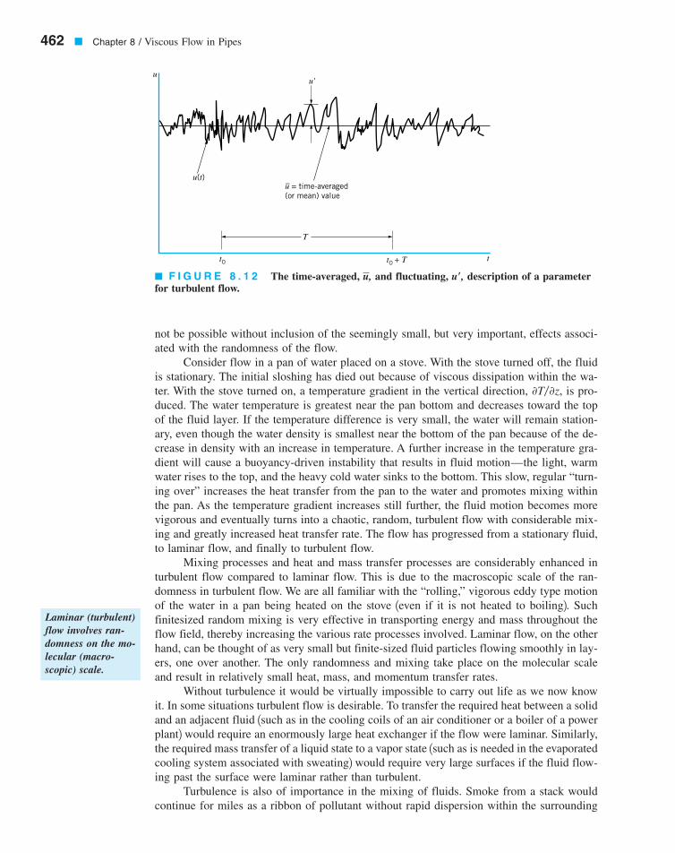
The fundamental difference between laminar and turbulent flow lies in the chaotic, randombehavior of the various fluid parameters. Such variations occur in the three components ofvelocity, the pressure, the shear stress, the temperature, and any other variable that has a fielddescription. Turbulent flow is characterized by random, three-dimensional vorticity 1i.e., fluidparticle rotation or spin; see Section 6.1.32. As is indicated in Fig. 8.12, such flows can bedescribed in terms of their mean values 1denoted with an overbar2 on which are superimposedthe fluctuations 1denoted with a prime2. Thus, if is the x component of in-stantaneous velocity, then its time mean 1or time average2 value, is
(8.24)
where the time interval, T, is considerably longer than the period of the longest fluctuations,but considerably shorter than any unsteadiness of the average velocity. This is illustrated inFig. 8.12.
The fluctuating part of the velocity, is that time-varying portion that differs fromthe average value
(8.25)
Clearly, the time average of the fluctuations is zero, since
The fluctuations are equally distributed on either side of the average. It is also clear, as is in-dicated in Fig. 8.13, that since the square of a fluctuation quantity cannot be negative
its average value is positive. Thus,
On the other hand, it may be that the average of products of the fluctuations, such as are zero or nonzero 1either positive or negative2.
The structure and characteristics of turbulence may vary from one flow situation to an-other. For example, the turbulence intensity 1or the level of the turbulence2 may be larger ina very gusty wind than it is in a relatively steady 1although turbulent2 wind. The turbulence
u¿ v¿,
1u¿ 22 �1
T �t0�T
t0
1u¿ 22 dt 7 0
3 1u¿ 22 0 4 ,
�1
T 1T u � T u 2 � 0
u¿ �1
T �
t0�T
t0
1u � u 2 dt �1
T a �
t0�T
t0
u dt � u �t0�T
t0
dtb
u � u � u¿ or u¿ � u � u
u¿
u �1
T �t0�T
t0
u1x, y, z, t2 dt
u,u � u1x, y, z, t2
8.3 Fully Developed Turbulent Flow � 463
Turbulent flow pa-rameters can be de-scribed in terms ofmean and fluctuat-ing portions.
7708d_c08_442-531 7/23/01 2:38 PM Page 463
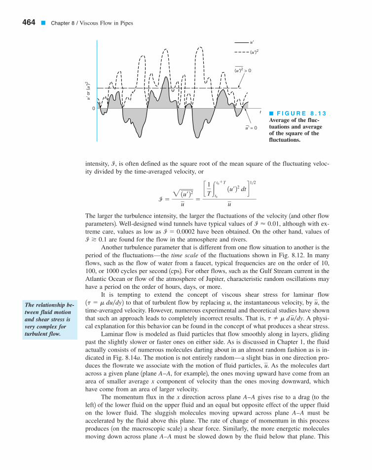
intensity, is often defined as the square root of the mean square of the fluctuating veloc-ity divided by the time-averaged velocity, or
The larger the turbulence intensity, the larger the fluctuations of the velocity 1and other flowparameters2. Well-designed wind tunnels have typical values of although with ex-treme care, values as low as have been obtained. On the other hand, values of
are found for the flow in the atmosphere and rivers.Another turbulence parameter that is different from one flow situation to another is the
period of the fluctuations—the time scale of the fluctuations shown in Fig. 8.12. In manyflows, such as the flow of water from a faucet, typical frequencies are on the order of 10,100, or 1000 cycles per second 1cps2. For other flows, such as the Gulf Stream current in theAtlantic Ocean or flow of the atmosphere of Jupiter, characteristic random oscillations mayhave a period on the order of hours, days, or more.
It is tempting to extend the concept of viscous shear stress for laminar flowto that of turbulent flow by replacing u, the instantaneous velocity, by the
time-averaged velocity. However, numerous experimental and theoretical studies have shownthat such an approach leads to completely incorrect results. That is, A physi-cal explanation for this behavior can be found in the concept of what produces a shear stress.
Laminar flow is modeled as fluid particles that flow smoothly along in layers, glidingpast the slightly slower or faster ones on either side. As is discussed in Chapter 1, the fluidactually consists of numerous molecules darting about in an almost random fashion as is in-dicated in Fig. 8.14a. The motion is not entirely random—a slight bias in one direction pro-duces the flowrate we associate with the motion of fluid particles, As the molecules dartacross a given plane 1plane A–A, for example2, the ones moving upward have come from anarea of smaller average x component of velocity than the ones moving downward, whichhave come from an area of larger velocity.
The momentum flux in the x direction across plane A–A gives rise to a drag 1to theleft2 of the lower fluid on the upper fluid and an equal but opposite effect of the upper fluidon the lower fluid. The sluggish molecules moving upward across plane A–A must beaccelerated by the fluid above this plane. The rate of change of momentum in this processproduces 1on the macroscopic scale2 a shear force. Similarly, the more energetic moleculesmoving down across plane A–A must be slowed down by the fluid below that plane. This
u.
t � m d u�dy.
u,1t � m du�dy2
i � 0.1i � 0.0002
i � 0.01,
i �2 1u¿ 22
u�
c 1T �
t0�T
t0
1u¿ 22 dt d 1�2
u
i,
464 � Chapter 8 / Viscous Flow in Pipes
(u')2 > 0
(u')2
u'
u' = 0
t
u' o
r (u
')2
0� F I G U R E 8 . 1 3Average of the fluc-tuations and average of the square of thefluctuations.
The relationship be-tween fluid motionand shear stress isvery complex forturbulent flow.
7708d_c08_442-531 7/23/01 2:38 PM Page 464
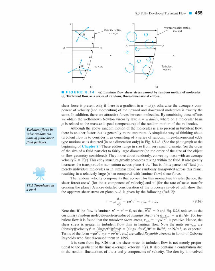
shear force is present only if there is a gradient in otherwise the average x com-ponent of velocity 1and momentum2 of the upward and downward molecules is exactly thesame. In addition, there are attractive forces between molecules. By combining these effectswe obtain the well-known Newton viscosity law: where on a molecular basis
is related to the mass and speed 1temperature2 of the random motion of the molecules.Although the above random motion of the molecules is also present in turbulent flow,
there is another factor that is generally more important. A simplistic way of thinking aboutturbulent flow is to consider it as consisting of a series of random, three-dimensional eddytype motions as is depicted 1in one dimension only2 in Fig. 8.14b. (See the photograph at thebeginning of Chapter 8.) These eddies range in size from very small diameter 1on the orderof the size of a fluid particle2 to fairly large diameter 1on the order of the size of the objector flow geometry considered2. They move about randomly, conveying mass with an averagevelocity This eddy structure greatly promotes mixing within the fluid. It also greatlyincreases the transport of x momentum across plane A–A. That is, finite parcels of fluid 1notmerely individual molecules as in laminar flow2 are randomly transported across this plane,resulting in a relatively large 1when compared with laminar flow2 shear force.
The random velocity components that account for this momentum transfer 1hence, theshear force2 are 1for the x component of velocity2 and 1for the rate of mass transfercrossing the plane2. A more detailed consideration of the processes involved will show thatthe apparent shear stress on plane A–A is given by the following 1Ref. 22:
(8.26)
Note that if the flow is laminar, so that and Eq. 8.26 reduces to thecustomary random molecule-motion-induced laminar shear stress, For tur-bulent flow it is found that the turbulent shear stress, is positive. Hence, theshear stress is greater in turbulent flow than in laminar flow. Note the units on are
or as expected.Terms of the form 1or etc.2 are called Reynolds stresses in honor of OsborneReynolds who first discussed them in 1895.
It is seen from Eq. 8.26 that the shear stress in turbulent flow is not merely propor-tional to the gradient of the time-averaged velocity, It also contains a contribution dueto the random fluctuations of the x and y components of velocity. The density is involved
u1y2.
�rv¿w¿,�ru¿v¿N�m2,1density2 1velocity22 � 1slugs�ft32 1ft�s22 � 1slugs # ft�s22�ft2 � lb�ft2,
tturb
tturb � �ru¿v¿,tlam � m d u�dy.
u¿v¿ � 0u¿ � v¿ � 0,
t � m d u
dy� ru¿v¿ � tlam � tturb
v¿u¿
u � u1y2.
m
t � m du�dy,
u � u1y2,
8.3 Fully Developed Turbulent Flow � 465
Turbulent flows in-volve random mo-tions of finite-sizedfluid particles.
u
AA
y
(1)
(2)
(a)
u1 < u2
Velocity profile, u = u(y)
u
AA
y
(b)
Turbulenteddies
Average velocity profile, u = u(y)
� F I G U R E 8 . 1 4 (a) Laminar flow shear stress caused by random motion of molecules.(b) Turbulent flow as a series of random, three-dimensional eddies.
V8.2 Turbulence ina bowl
7708d_c08_442-531 7/23/01 2:38 PM Page 465
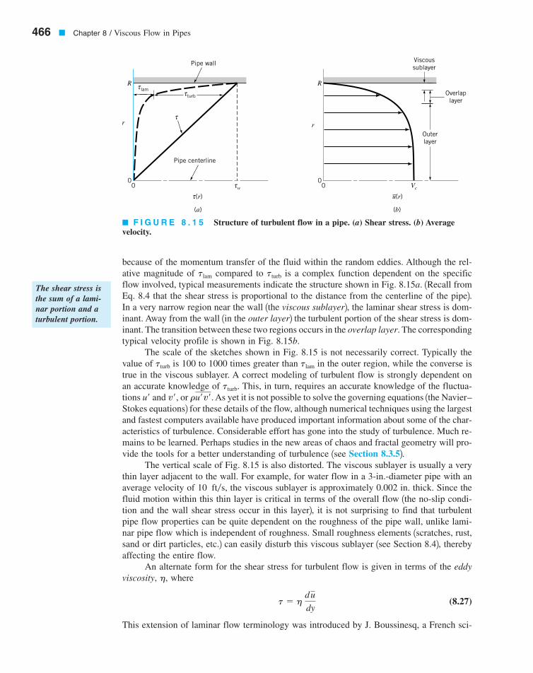
because of the momentum transfer of the fluid within the random eddies. Although the rel-ative magnitude of compared to is a complex function dependent on the specificflow involved, typical measurements indicate the structure shown in Fig. 8.15a. 1Recall fromEq. 8.4 that the shear stress is proportional to the distance from the centerline of the pipe2.In a very narrow region near the wall 1the viscous sublayer2, the laminar shear stress is dom-inant. Away from the wall 1in the outer layer2 the turbulent portion of the shear stress is dom-inant. The transition between these two regions occurs in the overlap layer. The correspondingtypical velocity profile is shown in Fig. 8.15b.
The scale of the sketches shown in Fig. 8.15 is not necessarily correct. Typically thevalue of is 100 to 1000 times greater than in the outer region, while the converse istrue in the viscous sublayer. A correct modeling of turbulent flow is strongly dependent onan accurate knowledge of This, in turn, requires an accurate knowledge of the fluctua-tions and or As yet it is not possible to solve the governing equations 1the Navier–Stokes equations2 for these details of the flow, although numerical techniques using the largestand fastest computers available have produced important information about some of the char-acteristics of turbulence. Considerable effort has gone into the study of turbulence. Much re-mains to be learned. Perhaps studies in the new areas of chaos and fractal geometry will pro-vide the tools for a better understanding of turbulence 1see Section 8.3.52.
The vertical scale of Fig. 8.15 is also distorted. The viscous sublayer is usually a verythin layer adjacent to the wall. For example, for water flow in a 3-in.-diameter pipe with anaverage velocity of the viscous sublayer is approximately 0.002 in. thick. Since thefluid motion within this thin layer is critical in terms of the overall flow 1the no-slip condi-tion and the wall shear stress occur in this layer2, it is not surprising to find that turbulentpipe flow properties can be quite dependent on the roughness of the pipe wall, unlike lami-nar pipe flow which is independent of roughness. Small roughness elements 1scratches, rust,sand or dirt particles, etc.2 can easily disturb this viscous sublayer 1see Section 8.42, therebyaffecting the entire flow.
An alternate form for the shear stress for turbulent flow is given in terms of the eddyviscosity, where
(8.27)
This extension of laminar flow terminology was introduced by J. Boussinesq, a French sci-
t � h du
dy
h,
10 ft�s,
ru¿v¿.v¿,u¿tturb.
tlamtturb
tturbtlam
466 � Chapter 8 / Viscous Flow in Pipes
Pipe wall
Pipe centerline
0
R
r
00
R
r
0ττ
τ
w
τ lamτ turb
(a) (b)
(r) u(r)
Vc
Outerlayer
Overlaplayer
Viscoussublayer
� F I G U R E 8 . 1 5 Structure of turbulent flow in a pipe. (a) Shear stress. (b) Average velocity.
The shear stress isthe sum of a lami-nar portion and aturbulent portion.
7708d_c08_442-531 7/23/01 2:38 PM Page 466
entist, in 1877. Although the concept of an eddy viscosity is intriguing, in practice it is notan easy parameter to use. Unlike the absolute viscosity, which is a known value for a givenfluid, the eddy viscosity is a function of both the fluid and the flow conditions. That is, theeddy viscosity of water cannot be looked up in handbooks—its value changes from one tur-bulent flow condition to another and from one point in a turbulent flow to another.
The inability to accurately determine the Reynolds stress, is equivalent to notknowing the eddy viscosity. Several semiempirical theories have been proposed 1Ref. 32 todetermine approximate values of L. Prandtl 11875–19532, a German physicist and aero-dynamicist, proposed that the turbulent process could be viewed as the random transport ofbundles of fluid particles over a certain distance, the mixing length, from a region of onevelocity to another region of a different velocity. By the use of some ad hoc assumptions andphysical reasoning, it was concluded that the eddy viscosity was given by
Thus, the turbulent shear stress is
(8.28)
The problem is thus shifted to that of determining the mixing length, Further considera-tions indicate that is not a constant throughout the flow field. Near a solid surface the tur-bulence is dependent on the distance from the surface. Thus, additional assumptions are maderegarding how the mixing length varies throughout the flow.
The net result is that as yet there is no general, all-encompassing, useful model thatcan accurately predict the shear stress throughout a general incompressible, viscous turbu-lent flow. Without such information it is impossible to integrate the force balance equationto obtain the turbulent velocity profile and other useful information, as was done for lami-nar flow.
8.3.3 Turbulent Velocity Profile
Considerable information concerning turbulent velocity profiles has been obtained throughthe use of dimensional analysis, experimentation, and semiempirical theoretical efforts. Asis indicated in Fig. 8.15, fully developed turbulent flow in a pipe can be broken into threeregions which are characterized by their distances from the wall: the viscous sublayer verynear the pipe wall, the overlap region, and the outer turbulent layer throughout the centerportion of the flow. Within the viscous sublayer the viscous shear stress is dominant com-pared with the turbulent 1or Reynolds2 stress, and the random, eddying nature of the flow isessentially absent. In the outer turbulent layer the Reynolds stress is dominant, and there isconsiderable mixing and randomness to the flow.
The character of the flow within these two regions is entirely different. For example,within the viscous sublayer the fluid viscosity is an important parameter; the density is unim-portant. In the outer layer the opposite is true. By a careful use of dimensional analysis ar-guments for the flow in each layer and by a matching of the results in the common overlaplayer, it has been possible to obtain the following conclusions about the turbulent velocityprofile in a smooth pipe 1Ref. 52.
In the viscous sublayer the velocity profile can be written in dimensionless form as
(8.29)
where is the distance measured from the wall, is the time-averaged x componentuy � R � r
u
u*�
yu*n
/m
/m.
tturb � r/2m adu
dyb2
h � r/m2 ` du
dy`
/m,
h.
ru¿v¿,
m,
8.3 Fully Developed Turbulent Flow � 467
Various ad hoc as-sumptions havebeen used to ap-proximate turbulentshear stresses.
7708d_c08_442-531 7/23/01 2:38 PM Page 467

of velocity, and is termed the friction velocity. Note that u* is not an actualvelocity of the fluid—it is merely a quantity that has dimensions of velocity. As is indicatedin Fig. 8.16, Eq. 8.29 1commonly called the law of the wall 2 is valid very near the smoothwall, for
Dimensional analysis arguments indicate that in the overlap region the velocity shouldvary as the logarithm of y. Thus, the following expression has been proposed:
(8.30)
where the constants 2.5 and 5.0 have been determined experimentally. As is indicated inFig. 8.16, for regions not too close to the smooth wall, but not all the way out to the pipecenter, Eq. 8.30 gives a reasonable correlation with the experimental data. Note that the hor-izontal scale is a logarithmic scale. This tends to exaggerate the size of the viscous sublayerrelative to the remainder of the flow. As is shown in Example 8.4, the viscous sublayer isusually quite thin. Similar results can be obtained for turbulent flow past rough walls1Ref. 172.
A number of other correlations exist for the velocity profile in turbulent pipe flow. Inthe central region 1the outer turbulent layer2 the expression where
is the centerline velocity, is often suggested as a good correlation with experimental data.Another often-used 1and relatively easy to use2 correlation is the empirical power-law velocityprofile
(8.31)
In this representation, the value of n is a function of the Reynolds number, as is indicated inFig. 8.17. The one-seventh power-law velocity profile is often used as a reasonableapproximation for many practical flows. Typical turbulent velocity profiles based on thispower-law representation are shown in Fig. 8.18.
1n � 72
u
Vc
� a1 �r
Rb1�n
Vc
1Vc � u2�u* � 2.5 ln1R�y2,
u
u*� 2.5 ln ayu*
nb � 5.0
0 yu*�n f 5.
u* � 1tw �r21�2
468 � Chapter 8 / Viscous Flow in Pipes
Experimental data
Eq. 8.29
Eq. 8.30Pipe
centerline
Viscoussublayer
01 10 102 103 104
5
10
15
20
25
u___u*
yu*____v
� F I G U R E 8 . 1 6Typical structure of the turbulent velocityprofile in a pipe.
A turbulent flow ve-locity profile can bedivided into variousregions.
7708d_c08_442-531 7/23/01 2:38 PM Page 468

A closer examination of Eq. 8.31 shows that the power-law profile cannot be valid nearthe wall, since according to this equation the velocity gradient is infinite there. In addition,Eq. 8.31 cannot be precisely valid near the centerline because it does not give at
However, it does provide a reasonable approximation to the measured velocity pro-files across most of the pipe.
Note from Fig. 8.18 that the turbulent profiles are much “flatter” than the laminar profileand that this flatness increases with Reynolds number 1i.e., with n2. Recall from Chapter 3that reasonable approximate results are often obtained by using the inviscid Bernoulli equa-tion and by assuming a fictitious uniform velocity profile. Since most flows are turbulent andturbulent flows tend to have nearly uniform velocity profiles, the usefulness of the Bernoulliequation and the uniform profile assumption is not unexpected. Of course, many propertiesof the flow cannot be accounted for without including viscous effects.
r � 0.du�dr � 0
8.3 Fully Developed Turbulent Flow � 469
A power-law veloc-ity profile approxi-mates the actualturbulent velocityprofile.
V8.3 Laminar/turbulent velocityprofiles
11
10
9
8n
7
5104
Re = VD____ρµ
105 106
6
1.0
0.5
00 0.5 1.0
Turbulent
Laminarn = 8
n = 6
n = 10
r__R
_u__Vc
� F I G U R E 8 . 1 7Exponent, n, forpower-law velocityprofiles. (Adaptedfrom Ref. 1.)
� F I G U R E 8 . 1 8 Typical laminar flow and turbulent flow velocity profiles.
7708d_c08_442-531 7/23/01 2:38 PM Page 469

470 � Chapter 8 / Viscous Flow in Pipes
EXAMPLE8.4
Water at and flows through a horizontal pipeof 0.1-m diameter with a flowrate of and a pressure gradient of2.59 kPa�m. 1a2 Determine the approximate thickness of the viscous sublayer. 1b2 Determinethe approximate centerline velocity, 1c2 Determine the ratio of the turbulent to laminarshear stress, at a point midway between the centerline and the pipe wall 1i.e., at
SOLUTION
(a) According to Fig. 8.16, the thickness of the viscous sublayer, is approximately
or
where
(1)
The wall shear stress can be obtained from the pressure drop data and Eq. 8.5, whichis valid for either laminar or turbulent flow. Thus,
Hence, from Eq. 1 we obtain
so that
(Ans)
As stated previously, the viscous sublayer is very thin. Minute imperfections on the pipewall will protrude into this sublayer and affect some of the characteristics of the flow1i.e., wall shear stress and pressure drop2.
(b) The centerline velocity can be obtained from the average velocity and the assumptionof a power-law velocity profile as follows. For this flow with
the Reynolds number is
Thus, from Fig. 8.17, so that
u
Vc
� a1 �r
Rb1�8.4
n � 8.4
Re �VDn
�15.09 m�s2 10.1 m211.004 � 10�6 m2�s2 � 5.07 � 105
V �Q
A�
0.04 m3�sp10.1 m22�4 � 5.09 m�s
ds �511.004 � 10�6 m2�s2
0.255 m�s� 1.97 � 10�5 m � 0.02 mm
u* � a64.8 N�m2
998 kg�m3b1�2
� 0.255 m�s
tw �D ¢p
4/�10.1 m2 12.59 � 103 N�m22
411 m2 � 64.8 N�m2
u* � atw
rb1�2
ds � 5 n
u*
dsu*n
� 5
ds,
r � 0.025 m2.tturb �tlam,Vc.
Q � 4 � 10�2 m3�sn � 1.004 � 10�6 m2�s220 °C 1r � 998 kg�m3
7708d_c08_442-531 7/23/01 2:38 PM Page 470

8.3 Fully Developed Turbulent Flow � 471
To determine the centerline velocity, we must know the relationship between V1the average velocity2 and This can be obtained by integration of the power-law ve-locity profile as follows. Since the flow is axisymmetric,
which can be integrated to give
Thus, since we obtain
With in the present case, this gives
(Ans)
Recall that for laminar pipe flow.(c) From Eq. 8.4, which is valid for laminar or turbulent flow, the shear stress at
is
or
where From the power-law velocity profile 1Eq. 8.312 we obtain thegradient of the average velocity as
which gives
Thus,
Thus, the ratio of turbulent to laminar shear stress is given by
(Ans)
As expected, most of the shear stress at this location in the turbulent flow is due to theturbulent shear stress.
tturb
tlam�t � tlam
tlam�
32.4 � 0.0266
0.0266� 1220
� 0.0266 N�m2
� �11.004 � 10�6 m2�s2 1998 kg�m32 1–26.5�s2 tlam � �m
du
dr� �1nr2 du
dr
du
dr� �
16.04 m�s28.410.05m2 a1 �
0.025 m
0.05 mb11�8.42�8.4
� �26.5�s
du
dr� �
Vc
nR a1 �
r
Rb11�n2�n
tlam � �m du�dr.
t � tlam � tturb � 32.4 N�m2
t �2twr
D�
2164.8 N�m22 10.025 m210.1 m2
r � 0.025 mVc � 2V
� 6.04 m�s
Vc �1n � 12 12n � 12
2n2 V � 1.186V � 1.186 15.09 m�s2n � 8.4
V
Vc
�2n2
1n � 12 12n � 12
Q � pR2V,
Q � 2pR2Vc n2
1n � 12 12n � 12
Q � AV � � u dA � Vc �r�R
r�0 a1 �
r
Rb1�n 12pr2 dr
Vc.Vc,
7708d_c08_442-531 7/23/01 2:38 PM Page 471

The turbulent flow characteristics discussed in this section are not unique to turbulentflow in round pipes. Many of the characteristics introduced 1i.e., the Reynolds stress, the vis-cous sublayer, the overlap layer, the outer layer, the general characteristics of the velocityprofile, etc.2 are found in other turbulent flows. In particular, turbulent pipe flow and turbu-lent flow past a solid wall 1boundary layer flow2 share many of these common traits. Suchideas are discussed more fully in Chapter 9.
8.3.4 Turbulence Modeling
Although it is not yet possible to theoretically predict the random, irregular details of turbu-lent flows, it would be useful to be able to predict the time-averaged flow fields 1pressure,velocity, etc.2 directly from the basic governing equations. To this end one can time averagethe governing Navier–Stokes equations 1Eqs. 6.31 and 6.1272 to obtain equations for theaverage velocity and pressure. However, because the Navier–Stokes equations are nonlinear,the resulting time-averaged differential equations contain not only the desired average pres-sure and velocity as variables, but also averages of products of the fluctuations—terms ofthe type that one tried to eliminate by averaging the equations! For example, the Reynoldsstress 1see Eq. 8.262 occurs in the time-averaged momentum equation.
Thus, it is not possible to merely average the basic differential equations and obtaingoverning equations involving only the desired averaged quantities. This is the reason for thevariety of ad hoc assumptions that have been proposed to provide “closure” to the equationsgoverning the average flow. That is, the set of governing equations must be a complete orclosed set of equations—the same number of equation as unknowns.
Various attempts have been made to solve this closure problem 1Refs. 1, 322. Suchschemes involving the introduction of an eddy viscosity or the mixing length 1as introducedin Section 8.3.22 are termed algebraic or zero-equation models. Other methods, which arebeyond the scope of this book, include the one-equation model and the two-equation model.These turbulence models are based on the equation for the turbulence kinetic energy and re-quire significant computer usage.
Turbulence modeling is an important and extremely difficult topic. Although consid-erable progress has been made, much remains to be done in this area.
8.3.5 Chaos and Turbulence
Chaos theory is a relatively new branch of mathematical physics that may provide insightinto the complex nature of turbulence. This method combines mathematics and numerical1computer2 techniques to provide a new way to analyze certain problems. Chaos theory, whichis quite complex and is only now being developed, involves the behavior of nonlinear dy-namical systems and their response to initial and boundary conditions. The flow of a viscousfluid, which is governed by the nonlinear Navier–Stokes equations 1Eq. 6.1272, may be sucha system.
To solve the Navier–Stokes equations for the velocity and pressure fields in a viscousflow, one must specify the particular flow geometry being considered 1the boundary condi-tions2 and the condition of the flow at some particular time 1the initial conditions2. If, as someresearchers predict, the Navier–Stokes equations allow chaotic behavior, then the state of theflow at times after the initial time may be very, very sensitive to the initial conditions. Aslight variation to the initial flow conditions may cause the flow at later times to be quitedifferent than it would have been with the original, only slightly different initial conditions.When carried to the extreme, the flow may be “chaotic,” “random,” or perhaps 1in currentterminology2, “turbulent.”
�ru¿v¿
472 � Chapter 8 / Viscous Flow in Pipes
Chaos theory mayeventually provide adeeper understand-ing of turbulence.
7708d_c08_442-531 7/23/01 2:38 PM Page 472

The occurrence of such behavior would depend on the value of the Reynolds number.For example, it may be found that for sufficiently small Reynolds numbers the flow is notchaotic 1i.e., it is laminar2, while for large Reynolds numbers it is chaotic with turbulent char-acteristics.
Thus, with the advancement of chaos theory it may be found that the numerous ad hocturbulence ideas mentioned in previous sections 1i.e., eddy viscosity, mixing length, law ofthe wall, etc.2 may not be needed. It may be that chaos theory can provide the turbulenceproperties and structure directly from the governing equations. As of now we must wait untilthis exciting topic is developed further. The interested reader is encouraged to consult Ref. 33for a general introduction to chaos or Ref. 34 for additional material.
8.4 Dimensional Analysis of Pipe Flow � 473
8.4 Dimensional Analysis of Pipe Flow
As was discussed in previous sections, turbulent flow can be a very complex, difficult topic—one that as yet has defied a rigorous theoretical treatment. Thus, most turbulent pipe flowanalyses are based on experimental data and semiempirical formulas, even if the flow is fullydeveloped. These results are given in dimensionless form and cover a very wide range offlow parameters, including arbitrary fluids, pipes, and flowrates. In addition to these fullydeveloped flow considerations, a variety of useful data are available regarding flow throughpipe fittings, such as elbows, tees, valves, and the like. These data are conveniently expressedin dimensionless form.
8.4.1 The Moody Chart
A dimensional analysis treatment of pipe flow provides the most convenient base from whichto consider turbulent, fully developed pipe flow. An introduction to this topic was given inSection 8.3. As is discussed in Sections 8.2.1 and 8.2.4, the pressure drop and head loss ina pipe are dependent on the wall shear stress, between the fluid and pipe surface. A fun-damental difference between laminar and turbulent flow is that the shear stress for turbulentflow is a function of the density of the fluid, For laminar flow, the shear stress is inde-pendent of the density, leaving the viscosity, as the only important fluid property.
Thus, the pressure drop, for steady, incompressible turbulent flow in a horizontalround pipe of diameter D can be written in functional form as
(8.32)
where V is the average velocity, is the pipe length, and is a measure of the roughness ofthe pipe wall. It is clear that should be a function of V, D, and The dependence of on the fluid properties and is expected because of the dependence of on these parameters.
Although the pressure drop for laminar pipe flow is found to be independent of theroughness of the pipe, it is necessary to include this parameter when considering turbulentflow. As is discussed in Section 8.3.3 and illustrated in Fig. 8.19, for turbulent flow there isa relatively thin viscous sublayer formed in the fluid near the pipe wall. In many instancesthis layer is very thin; where is the sublayer thickness. If a typical wall rough-ness element protrudes sufficiently far into 1or even through2 this layer, the structure and prop-erties of the viscous sublayer 1along with and 2 will be different than if the wall weresmooth. Thus, for turbulent flow the pressure drop is expected to be a function of the wallroughness. For laminar flow there is no thin viscous layer–viscous effects are important acrossthe entire pipe. Thus, relatively small roughness elements have completely negligible effectson laminar pipe flow. Of course, for pipes with very large wall “roughness,”such as that in corrugated pipes, the flowrate may be a function of the “roughness.” We willconsider only typical constant diameter pipes with relative roughnesses in the range
1e�D g 0.12,
tw¢p
dsds�D 1,
trm
¢p/.¢pe/
¢p � F1V, D, /, e, m, r2¢p,
m,r.
tw,
Most turbulent pipeflow information isbased on experi-mental data.
7708d_c08_442-531 7/23/01 2:38 PM Page 473
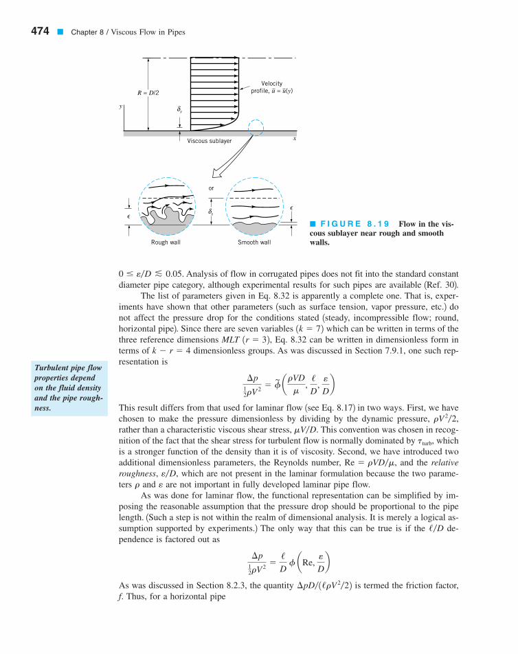
Analysis of flow in corrugated pipes does not fit into the standard constantdiameter pipe category, although experimental results for such pipes are available 1Ref. 302.
The list of parameters given in Eq. 8.32 is apparently a complete one. That is, exper-iments have shown that other parameters 1such as surface tension, vapor pressure, etc.2 donot affect the pressure drop for the conditions stated 1steady, incompressible flow; round,horizontal pipe2. Since there are seven variables which can be written in terms of thethree reference dimensions MLT Eq. 8.32 can be written in dimensionless form interms of dimensionless groups. As was discussed in Section 7.9.1, one such rep-resentation is
This result differs from that used for laminar flow 1see Eq. 8.172 in two ways. First, we havechosen to make the pressure dimensionless by dividing by the dynamic pressure,rather than a characteristic viscous shear stress, This convention was chosen in recog-nition of the fact that the shear stress for turbulent flow is normally dominated by whichis a stronger function of the density than it is of viscosity. Second, we have introduced twoadditional dimensionless parameters, the Reynolds number, and the relativeroughness, which are not present in the laminar formulation because the two parame-ters and are not important in fully developed laminar pipe flow.
As was done for laminar flow, the functional representation can be simplified by im-posing the reasonable assumption that the pressure drop should be proportional to the pipelength. 1Such a step is not within the realm of dimensional analysis. It is merely a logical as-sumption supported by experiments.2 The only way that this can be true is if the de-pendence is factored out as
As was discussed in Section 8.2.3, the quantity is termed the friction factor,f. Thus, for a horizontal pipe
¢pD� 1/rV 2�22
¢p12rV
2�
/D
f aRe, e
Db
/�D
er
e�D,Re � rVD�m,
tturb,mV�D.
rV 2�2,
¢p12rV
2� f
~ arVDm
, /D
, e
Db
k � r � 41r � 32, 1k � 72
0 e�D f 0.05.
474 � Chapter 8 / Viscous Flow in Pipes
R = D/2
δs
δs
Viscous sublayer
Velocityprofile, u = u(y)
y
x
∋∋
Smooth wallRough wall
or
� F I G U R E 8 . 1 9 Flow in the vis-cous sublayer near rough and smoothwalls.
Turbulent pipe flowproperties dependon the fluid densityand the pipe rough-ness.
7708d_c08_442-531 7/23/01 2:38 PM Page 474
8.4 Dimensional Analysis of Pipe Flow � 475
(8.33)
where
For laminar fully developed flow, the value of f is simply independent of For turbulent flow, the functional dependence of the friction factor on the Reynolds numberand the relative roughness, is a rather complex one that cannot, as yet, beobtained from a theoretical analysis. The results are obtained from an exhaustive set of ex-periments and usually presented in terms of a curve-fitting formula or the equivalent graph-ical form.
From Eq. 5.89 the energy equation for steady incompressible flow is
where is the head loss between sections 112 and 122. With the assumption of a constant di-ameter so that horizontal pipe with fully developed flow
this becomes which can be combined with Eq. 8.33 to give
(8.34)
Equation 8.34, called the Darcy–Weisbach equation, is valid for any fully developed, steady,incompressible pipe flow—whether the pipe is horizontal or on a hill. On the other hand,Eq. 8.33 is valid only for horizontal pipes. In general, with the energy equation gives
Part of the pressure change is due to the elevation change and part is due to the head lossassociated with frictional effects, which are given in terms of the friction factor, f.
It is not easy to determine the functional dependence of the friction factor on theReynolds number and relative roughness. Much of this information is a result of experimentsconducted by J. Nikuradse in 1933 1Ref. 62 and amplified by many others since then. Onedifficulty lies in the determination of the roughness of the pipe. Nikuradse used artificiallyroughened pipes produced by gluing sand grains of known size onto pipe walls to producepipes with sandpaper-type surfaces. The pressure drop needed to produce a desired flowratewas measured and the data were converted into the friction factor for the correspondingReynolds number and relative roughness. The tests were repeated numerous times for a widerange of Re and to determine the dependence.
In commercially available pipes the roughness is not as uniform and well defined asin the artificially roughened pipes used by Nikuradse. However, it is possible to obtain a mea-sure of the effective relative roughness of typical pipes and thus to obtain the friction factor.Typical roughness values for various pipe surfaces are given in Table 8.1. Figure 8.20 showsthe functional dependence of f on Re and and is called the Moody chart in honor ofL. F. Moody, who, along with C. F. Colebrook, correlated the original data of Nikuradse interms of the relative roughness of commercially available pipe materials. It should be notedthat the values of do not necessarily correspond to the actual values obtained by a e�D
e�D
f � f1Re, e�D2e�D
p1 � p2 � g1z2 � z12 � ghL � g1z2 � z12 � f /D
rV 2
2
V1 � V2
hL � f /D
V 2
2g
¢p � p1 � p2 � ghL,1a1 � a22,1z1 � z22V1 � V22,1D1 � D2
hL
p1
g� a1
V 12
2g� z1 �
p2
g� a2
V 22
2g� z2 � hL
f � f1Re, e�D2,e�D.f � 64�Re,
f � f aRe, e
Db
¢p � f /D
rV 2
2
The head loss inpipe flow is given interms of the frictionfactor.
7708d_c08_442-531 7/23/01 2:38 PM Page 475
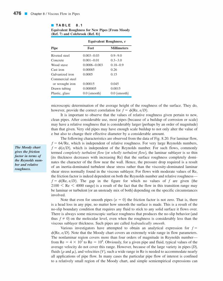
microscopic determination of the average height of the roughness of the surface. They do,however, provide the correct correlation for
It is important to observe that the values of relative roughness given pertain to new,clean pipes. After considerable use, most pipes 1because of a buildup of corrosion or scale2may have a relative roughness that is considerably larger 1perhaps by an order of magnitude2than that given. Very old pipes may have enough scale buildup to not only alter the value of
but also to change their effective diameter by a considerable amount.The following characteristics are observed from the data of Fig. 8.20. For laminar flow,
which is independent of relative roughness. For very large Reynolds numbers,which is independent of the Reynolds number. For such flows, commonly
termed completely turbulent flow 1or wholly turbulent flow2, the laminar sublayer is so thin1its thickness decreases with increasing Re2 that the surface roughness completely domi-nates the character of the flow near the wall. Hence, the pressure drop required is a resultof an inertia-dominated turbulent shear stress rather than the viscosity-dominated laminarshear stress normally found in the viscous sublayer. For flows with moderate values of Re,the friction factor is indeed dependent on both the Reynolds number and relative roughness—
The gap in the figure for which no values of f are given 1therange2 is a result of the fact that the flow in this transition range may
be laminar or turbulent 1or an unsteady mix of both2 depending on the specific circumstancesinvolved.
Note that even for smooth pipes the friction factor is not zero. That is, thereis a head loss in any pipe, no matter how smooth the surface is made. This is a result of theno-slip boundary condition that requires any fluid to stick to any solid surface it flows over.There is always some microscopic surface roughness that produces the no-slip behavior 1andthus 2 on the molecular level, even when the roughness is considerably less than theviscous sublayer thickness. Such pipes are called hydraulically smooth.
Various investigators have attempted to obtain an analytical expression for Note that the Moody chart covers an extremely wide range in flow parameters.
The nonlaminar region covers more than four orders of magnitude in Reynolds number—from to Obviously, for a given pipe and fluid, typical values of theaverage velocity do not cover this range. However, because of the large variety in pipes 1D2,fluids and and velocities 1V 2, such a wide range in Re is needed to accommodate nearlyall applications of pipe flow. In many cases the particular pipe flow of interest is confinedto a relatively small region of the Moody chart, and simple semiempirical expressions can
m2,1rRe � 108.Re � 4 � 103
f1Re, e�D2.f �
f � 0
1e � 02
2100 6 Re 6 4000f � f1Re, e�D2.
f � f1e�D2,f � 64�Re,
e
f � f1Re, e�D2.
476 � Chapter 8 / Viscous Flow in Pipes
� TA B L E 8 . 1Equivalent Roughness for New Pipes [From Moody(Ref. 7) and Colebrook (Ref. 8)]
Equivalent Roughness,
Pipe Feet Millimeters
Riveted steel 0.003–0.03 0.9–9.0Concrete 0.001–0.01 0.3–3.0Wood stave 0.0006–0.003 0.18–0.9Cast iron 0.00085 0.26Galvanized iron 0.0005 0.15Commercial steelor wrought iron 0.00015 0.045
Drawn tubing 0.000005 0.0015Plastic, glass 0.0 1smooth2 0.0 1smooth2
E
The Moody chartgives the frictionfactor in terms ofthe Reynolds num-ber and relativeroughness.
7708d_c08_442-531 7/23/01 2:38 PM Page 476

477
Transition range
Laminarflow
Smooth
Wholly turbulent flow
0.1
0.09
0.08
0.07
0.06
0.05
0.04
0.03
0.025
0.02
0.015
0.01
0.009
0.008
103
2(103) 4 6 8
104
2(104) 4 6 8
105
2(105) 4 6 8
106
2(106) 4 6 8
107
2(107) 4 6 8
0.050.04
0.03
0.02
0.015
0.010.008
0.006
0.004
0.002
0.0010.00080.0006
0.0004
0.0002
0.0001
0.00005
0.00001
f
Re = VD
_____µ
ρ
__D
∋
� F I G U R E 8 . 2 0 Friction factor as a function of Reynolds number and relative roughness for round pipes—the Moodychart. (Data from Ref. 7 with permission.)
7708d_c08_442-531 7/23/01 2:38 PM Page 477

be developed for those conditions. For example, a company that manufactures cast iron wa-ter pipes with diameters between 2 and 12 in. may use a simple equation valid for their con-ditions only. The Moody chart, on the other hand, is universally valid for all steady, fully de-veloped, incompressible pipe flows.
The following equation from Colebrook is valid for the entire nonlaminar range of theMoody chart
(8.35)
In fact, the Moody chart is a graphical representation of this equation, which is an empiri-cal fit of the pipe flow pressure drop data. Equation 8.35 is called the Colebrook formula. Adifficulty with its use is that it is implicit in the dependence of f. That is, for given condi-tions it is not possible to solve for f without some sort of iterative scheme.With the use of modern computers and calculators, such calculations are not difficult. 1Asshown in Problem 8.37 at the end of this chapter, it is possible to obtain an equation thatadequately approximates the Colebrook�Moody chart relationship but does not require aniterative scheme.2 A word of caution is in order concerning the use of the Moody chart orthe equivalent Colebrook formula. Because of various inherent inaccuracies involved 1un-certainty in the relative roughness, uncertainty in the experimental data used to produce theMoody chart, etc.2, the use of several place accuracy in pipe flow problems is usually notjustified. As a rule of thumb, a 10% accuracy is the best expected.
1Re and e�D2,
11f� �2.0 log ae�D
3.7�
2.51
Re1fb
478 � Chapter 8 / Viscous Flow in Pipes
EXAMPLE8.5
The turbulent por-tion of the Moodychart is representedby the Colebrookformula.
Air under standard conditions flows through a 4.0-mm-diameter drawn tubing with an aver-age velocity of For such conditions the flow would normally be turbulent. How-ever, if precautions are taken to eliminate disturbances to the flow 1the entrance to the tubeis very smooth, the air is dust free, the tube does not vibrate, etc.2, it may be possible tomaintain laminar flow. 1a2 Determine the pressure drop in a 0.1-m section of the tube if theflow is laminar. 1b2 Repeat the calculations if the flow is turbulent.
SOLUTION
Under standard temperature and pressure conditions the density and viscosity areand Thus, the Reynolds number is
which would normally indicate turbulent flow.
(a) If the flow were laminar, then and the pressuredrop in a 0.1-m-long horizontal section of the pipe would be
or
(Ans)
Note that the same result is obtained from Eq. 8.8.
¢p �32m/
D2 V �3211.79 � 10�5 N # s�m22 10.1 m2 150 m�s2
10.004 m22 � 179 N�m2
¢p � 0.179 kPa
¢p � f /D
1
2 rV 2 � 10.004672 10.1 m2
10.004 m2 1
2 11.23 kg�m32 150 m�s22
f � 64�Re � 64�13,700 � 0.00467
Re �rVDm
�11.23 kg�m32 150 m�s2 10.004 m2
1.79 � 10�5 N # s�m2 � 13,700
m � 1.79 � 10�5 N # s�m2.r � 1.23 kg�m3
V � 50 m�s
7708d_c08_478 7/24/01 11:10 AM Page 478

8.4 Dimensional Analysis of Pipe Flow � 479
(b) If the flow were turbulent, then where from Table 8.1,so that From the Moody chart with
we obtain Thus, the pressure drop in thiscase would be approximately
or
(Ans)
A considerable savings in effort to force the fluid through the pipe could be realized10.179 kPa rather than 1.076 kPa2 if the flow could be maintained as laminar flow atthis Reynolds number. In general this is very difficult to do, although laminar flow inpipes has been maintained up to in rare instances.
An alternate method to determine the friction factor for the turbulent flow wouldbe to use the Colebrook formula, Eq. 8.35. Thus,
or
(1)
An iterative procedure to obtain f can be done as follows. We assume a value of f1 for example2, substitute it into the right-hand side of Eq. 1, and calculate anew f 1 in this case2. Since the two values do not agree, the assumed valueis not the solution. Hence, we try again. This time we assume 1the last valuecalculated2 and calculate the new value as Again this is still not the solu-tion. Two more iterations show that the assumed and calculated values converge to thesolution in agreement 1within the accuracy of reading the graph2 with theMoody chart method of
Numerous other empirical formulas can be found in the literature 1Ref. 52 for por-tions of the Moody chart. For example, an often-used equation, commonly referred toas the Blasius formula, for turbulent flow in smooth pipes with is
For our case this gives
which is in agreement with the previous results. Note that the value of f is relatively in-sensitive to for this particular situation. Whether the tube was smooth glass
or the drawn tubing would not make much difference inthe pressure drop. For this flow, an increase in relative roughness by a factor of 30 to1equivalent to a commercial steel surface; see Table 8.12 would give
This would represent an increase in pressure drop and head loss by a fac-tor of compared with that for the original drawn tubing.
The pressure drop of 1.076 kPa in a length of 0.1 m of pipe corresponds to a change in absolute pressure [assuming ] of approximately p � 101 kPa 1abs2 at x � 0
0.043�0.0291 � 1.48f � 0.043.e�D � 0.0113
1e�D � 0.00037521e�D � 02 e�D
f � 0.316113,7002�0.25 � 0.0292
f �0.316
Re1�4
Re 6 1051e�D � 02
f � 0.028.f � 0.0291,
f � 0.0289.f � 0.0307
f � 0.0307f � 0.02,
11f� �2.0 log a1.01 � 10�4 �
1.83 � 10�41fb
11f� �2.0 log ae�D
3.7�
2.51
Re1fb � �2.0 log a0.000375
3.7�
2.51
1.37 � 1041fb
Re � 100,000
¢p � 1.076 kPa
¢p � f /D
1
2 rV 2 � 10.0282 10.1 m2
10.004 m2 1
2 11.23 kg�m32 150 m�s22
f � 0.028.1.37 � 104 and e�D � 0.000375Re �e�D � 0.0015 mm�4.0 mm � 0.000375.
e � 0.0015 mmf � f1Re, e�D2,
7708d_c08_479 8/16/01 5:09 PM Page 479
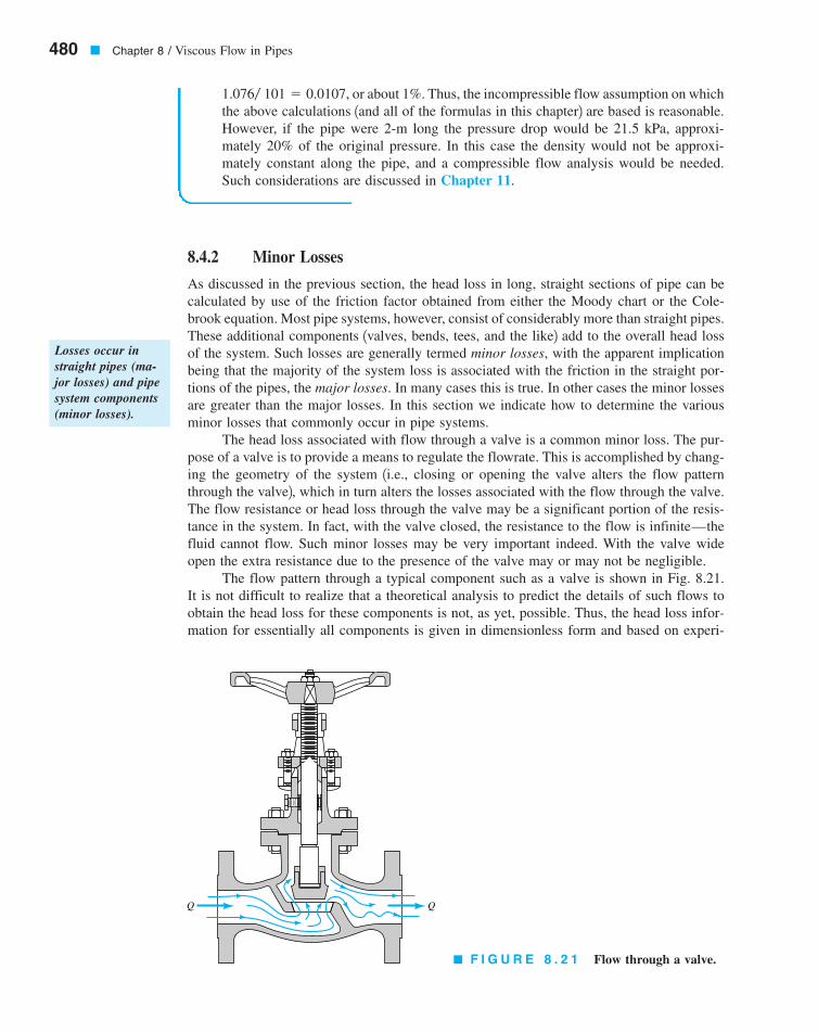
8.4.2 Minor Losses
As discussed in the previous section, the head loss in long, straight sections of pipe can becalculated by use of the friction factor obtained from either the Moody chart or the Cole-brook equation. Most pipe systems, however, consist of considerably more than straight pipes.These additional components 1valves, bends, tees, and the like2 add to the overall head lossof the system. Such losses are generally termed minor losses, with the apparent implicationbeing that the majority of the system loss is associated with the friction in the straight por-tions of the pipes, the major losses. In many cases this is true. In other cases the minor lossesare greater than the major losses. In this section we indicate how to determine the variousminor losses that commonly occur in pipe systems.
The head loss associated with flow through a valve is a common minor loss. The pur-pose of a valve is to provide a means to regulate the flowrate. This is accomplished by chang-ing the geometry of the system 1i.e., closing or opening the valve alters the flow patternthrough the valve2, which in turn alters the losses associated with the flow through the valve.The flow resistance or head loss through the valve may be a significant portion of the resis-tance in the system. In fact, with the valve closed, the resistance to the flow is infinite—thefluid cannot flow. Such minor losses may be very important indeed. With the valve wideopen the extra resistance due to the presence of the valve may or may not be negligible.
The flow pattern through a typical component such as a valve is shown in Fig. 8.21.It is not difficult to realize that a theoretical analysis to predict the details of such flows toobtain the head loss for these components is not, as yet, possible. Thus, the head loss infor-mation for essentially all components is given in dimensionless form and based on experi-
480 � Chapter 8 / Viscous Flow in Pipes
or about 1%. Thus, the incompressible flow assumption on whichthe above calculations 1and all of the formulas in this chapter2 are based is reasonable.However, if the pipe were 2-m long the pressure drop would be 21.5 kPa, approxi-mately 20% of the original pressure. In this case the density would not be approxi-mately constant along the pipe, and a compressible flow analysis would be needed.Such considerations are discussed in Chapter 11.
101 � 0.0107,1.076�
Q Q
� F I G U R E 8 . 2 1 Flow through a valve.
Losses occur instraight pipes (ma-jor losses) and pipesystem components(minor losses).
7708d_c08_480 8/16/01 5:09 PM Page 480
mental data. The most common method used to determine these head losses or pressure dropsis to specify the loss coefficient, which is defined as
so that
or
(8.36)
The pressure drop across a component that has a loss coefficient of is equal to thedynamic pressure,
The actual value of is strongly dependent on the geometry of the component con-sidered. It may also be dependent on the fluid properties. That is,
where is the pipe Reynolds number. For many practical applications theReynolds number is large enough so that the flow through the component is dominated byinertia effects, with viscous effects being of secondary importance. This is true because ofthe relatively large accelerations and decelerations experienced by the fluid as it flows alonga rather curved, variable-area 1perhaps even torturous2 path through the component 1seeFig. 8.212. In a flow that is dominated by inertia effects rather than viscous effects, it is usu-ally found that pressure drops and head losses correlate directly with the dynamic pressure.This is the reason why the friction factor for very large Reynolds number, fully developedpipe flow is independent of the Reynolds number. The same condition is found to be true forflow through pipe components. Thus, in most cases of practical interest the loss coefficientsfor components are a function of geometry only,
Minor losses are sometimes given in terms of an equivalent length, In this termi-nology, the head loss through a component is given in terms of the equivalent length of pipethat would produce the same head loss as the component. That is,
or
where D and f are based on the pipe containing the component. The head loss of the pipesystem is the same as that produced in a straight pipe whose length is equal to the pipes ofthe original system plus the sum of the additional equivalent lengths of all of the compo-nents of the system. Most pipe flow analyses, including those in this book, use the loss co-efficient method rather than the equivalent length method to determine the minor losses.
Many pipe systems contain various transition sections in which the pipe diameterchanges from one size to another. Such changes may occur abruptly or rather smoothlythrough some type of area change section. Any change in flow area contributes losses thatare not accounted for in the fully developed head loss calculation 1the friction factor2. Theextreme cases involve flow into a pipe from a reservoir 1an entrance2 or out of a pipe into areservoir 1an exit2.
/eq �KLD
f
hL � KL V 2
2g� f
/eq
D V 2
2g
/eq.KL � f1geometry2.
Re � rVD�m
KL � f1geometry, Re2KL
rV 2�2.KL � 1
hL � KL V 2
2g
¢p � KL 12rV2
KL �hL
1V 2�2g2 �¢p
12rV
2
KL,
8.4 Dimensional Analysis of Pipe Flow � 481
Losses due to pipesystem componentsare given in termsof loss coefficients.
7708d_c08_442-531 7/23/01 2:38 PM Page 481

A fluid may flow from a reservoir into a pipe through any number of different shapedentrance regions as are sketched in Fig. 8.22. Each geometry has an associated loss coeffi-cient. A typical flow pattern for flow entering a pipe through a square-edged entrance issketched in Fig. 8.23. As was discussed in Chapter 3, a vena contracta region may result
482 � Chapter 8 / Viscous Flow in Pipes
(a) (b)
(c) (d)
Vena contracta
(2) (3)(1) V2 > V3
xV1 = 0
Flow separationat corner
Separated flow
(a)
p1
p3
x1 x2 x3 x
p
(b)
Actual
Ideal full recoveryof kinetic energy
V 22____
2
ρ
V 23____
2
ρ
V 23____
2
ρKL
� F I G U R E 8 . 2 2 Entrance flow conditions and loss coefficient (Refs. 28, 29). (a) Reen-trant, (b) sharp-edged, (c) slightly rounded, (see Fig. 8.24),KL � 0.2KL � 0.5,KL � 0.8,
� F I G U R E 8 . 2 3 Flow pattern and pressure distribution for a sharp-edged entrance.
(d) well-rounded, (see Fig. 8.24).KL � 0.04
A vena contractaregion is often de-veloped at the en-trance to a pipe.
7708d_c08_442-531 7/23/01 2:38 PM Page 482

because the fluid cannot turn a sharp right-angle corner. The flow is said to separate fromthe sharp corner. The maximum velocity at section 122 is greater than that in the pipe at sec-tion 132, and the pressure there is lower. If this high-speed fluid could slow down efficiently,the kinetic energy could be converted into pressure 1the Bernoulli effect2, and the ideal pres-sure distribution indicated in Fig. 8.23 would result. The head loss for the entrance wouldbe essentially zero.
Such is not the case. Although a fluid may be accelerated very efficiently, it is verydifficult to slow down 1decelerate2 a fluid efficiently. Thus, the extra kinetic energy of thefluid at section 122 is partially lost because of viscous dissipation, so that the pressure doesnot return to the ideal value. An entrance head loss 1pressure drop2 is produced as is indi-cated in Fig. 8.23. The majority of this loss is due to inertia effects that are eventually dis-sipated by the shear stresses within the fluid. Only a small portion of the loss is due to thewall shear stress within the entrance region. The net effect is that the loss coefficient for asquare-edged entrance is approximately One-half of a velocity head is lost as thefluid enters the pipe. If the pipe protrudes into the tank 1a reentrant entrance2 as is shown inFig. 8.22a, the losses are even greater.
KL � 0.50.
8.4 Dimensional Analysis of Pipe Flow � 483
D
r
0.5
0.4
0.3
0.2
0.1
00 0.05 0.1 0.15 0.20 0.25
r__D
KL
(a)
(c) (d)
(b)
(1)
(2)
� F I G U R E 8 . 2 4Entrance loss coefficient asa function of rounding ofthe inlet edge (Ref. 9).
� F I G U R E 8 . 2 5 Exit flow conditions and loss coefficient. (a) Reentrant,
(b) sharp-edged, (c) slightly rounded, (d) well-rounded, KL � 1.0.KL � 1.0,KL � 1.0,
KL � 1.0,
V8.4 Entrance/exitflows
Minor head lossesare often a result ofthe dissipation ofkinetic energy.
7708d_c08_442-531 7/23/01 2:38 PM Page 483
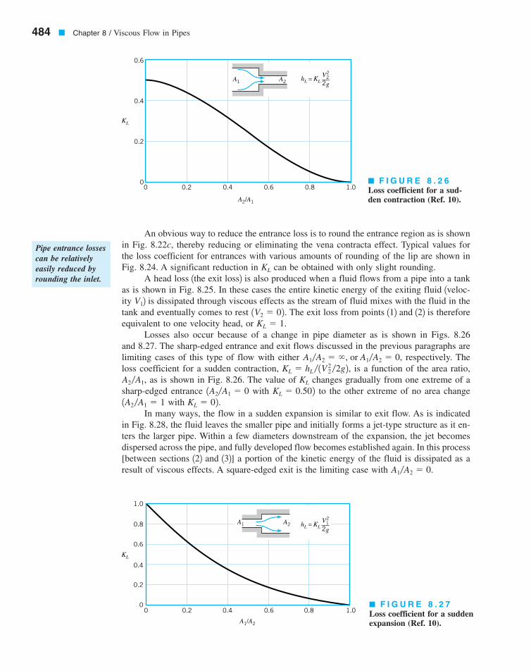
An obvious way to reduce the entrance loss is to round the entrance region as is shownin Fig. 8.22c, thereby reducing or eliminating the vena contracta effect. Typical values forthe loss coefficient for entrances with various amounts of rounding of the lip are shown inFig. 8.24. A significant reduction in can be obtained with only slight rounding.
A head loss 1the exit loss2 is also produced when a fluid flows from a pipe into a tankas is shown in Fig. 8.25. In these cases the entire kinetic energy of the exiting fluid 1veloc-ity 2 is dissipated through viscous effects as the stream of fluid mixes with the fluid in thetank and eventually comes to rest The exit loss from points 112 and 122 is thereforeequivalent to one velocity head, or
Losses also occur because of a change in pipe diameter as is shown in Figs. 8.26and 8.27. The sharp-edged entrance and exit flows discussed in the previous paragraphs arelimiting cases of this type of flow with either respectively. Theloss coefficient for a sudden contraction, is a function of the area ratio,
as is shown in Fig. 8.26. The value of changes gradually from one extreme of asharp-edged entrance with to the other extreme of no area change
with In many ways, the flow in a sudden expansion is similar to exit flow. As is indicated
in Fig. 8.28, the fluid leaves the smaller pipe and initially forms a jet-type structure as it en-ters the larger pipe. Within a few diameters downstream of the expansion, the jet becomesdispersed across the pipe, and fully developed flow becomes established again. In this process[between sections 122 and 132] a portion of the kinetic energy of the fluid is dissipated as aresult of viscous effects. A square-edged exit is the limiting case with A1�A2 � 0.
KL � 02.1A2�A1 � 1KL � 0.5021A2�A1 � 0
KLA2�A1,KL � hL � 1V 2
2 �2g2,A1�A2 � �, or A1�A2 � 0,
KL � 1.1V2 � 02.V1
KL
484 � Chapter 8 / Viscous Flow in Pipes
A1 A2 hL = KL V2
2___2g
0.6
0.4
0.2
00 0.2 0.4 0.6 0.8 1.0
A2/A1
KL
A1 A2 hL = KL V1
2___2g
1.0
0.8
0.6
0.4
0.2
00 0.2 0.4 0.6 0.8 1.0
A1/A2
KL
� F I G U R E 8 . 2 6Loss coefficient for a sud-den contraction (Ref. 10).
� F I G U R E 8 . 2 7Loss coefficient for a suddenexpansion (Ref. 10).
Pipe entrance lossescan be relativelyeasily reduced byrounding the inlet.
7708d_c08_442-531 7/23/01 2:38 PM Page 484
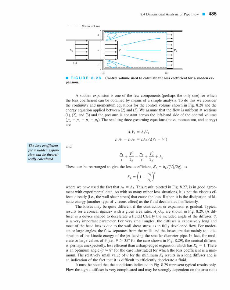
A sudden expansion is one of the few components 1perhaps the only one2 for whichthe loss coefficient can be obtained by means of a simple analysis. To do this we considerthe continuity and momentum equations for the control volume shown in Fig. 8.28 and theenergy equation applied between 122 and 132. We assume that the flow is uniform at sections112, 122, and 132 and the pressure is constant across the left-hand side of the control volume
The resulting three governing equations 1mass, momentum, and energy2are
and
These can be rearranged to give the loss coefficient, as
where we have used the fact that This result, plotted in Fig. 8.27, is in good agree-ment with experimental data. As with so many minor loss situations, it is not the viscous ef-fects directly 1i.e., the wall shear stress2 that cause the loss. Rather, it is the dissipation of ki-netic energy 1another type of viscous effect2 as the fluid decelerates inefficiently.
The losses may be quite different if the contraction or expansion is gradual. Typicalresults for a conical diffuser with a given area ratio, are shown in Fig. 8.29. 1A dif-fuser is a device shaped to decelerate a fluid.2 Clearly the included angle of the diffuser,is a very important parameter. For very small angles, the diffuser is excessively long andmost of the head loss is due to the wall shear stress as in fully developed flow. For moder-ate or large angles, the flow separates from the walls and the losses are due mainly to a dis-sipation of the kinetic energy of the jet leaving the smaller diameter pipe. In fact, for mod-erate or large values of 1i.e., for the case shown in Fig. 8.292, the conical diffuseris, perhaps unexpectedly, less efficient than a sharp-edged expansion which has Thereis an optimum angle 1 for the case illustrated2 for which the loss coefficient is a min-imum. The relatively small value of for the minimum results in a long diffuser and isan indication of the fact that it is difficult to efficiently decelerate a fluid.
It must be noted that the conditions indicated in Fig. 8.29 represent typical results only.Flow through a diffuser is very complicated and may be strongly dependent on the area ratio
KLu
u � 8°KL � 1.
u 7 35°u
u,A2�A1,
A2 � A3.
KL � a1 �A1
A2b2
KL � hL � 1V 21�2g2,
p1
g�
V 21
2g�
p3
g�
V 23
2g� hL
p1A3 � p3A3 � rA3V31V3 � V12 A1V1 � A3V3
1pa � pb � pc � p12.
8.4 Dimensional Analysis of Pipe Flow � 485
The loss coefficientfor a sudden expan-sion can be theoret-ically calculated.
(2) (3)
(1)
V1 V1 V3b
c
a
Control volume
� F I G U R E 8 . 2 8 Control volume used to calculate the loss coefficient for a sudden ex-pansion.
7708d_c08_442-531 7/23/01 2:38 PM Page 485
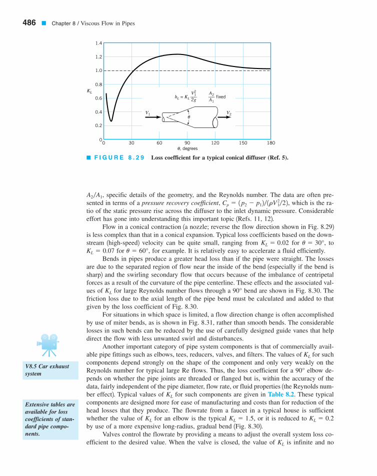
specific details of the geometry, and the Reynolds number. The data are often pre-sented in terms of a pressure recovery coefficient, which is the ra-tio of the static pressure rise across the diffuser to the inlet dynamic pressure. Considerableeffort has gone into understanding this important topic 1Refs. 11, 122.
Flow in a conical contraction 1a nozzle; reverse the flow direction shown in Fig. 8.292is less complex than that in a conical expansion. Typical loss coefficients based on the down-stream 1high-speed2 velocity can be quite small, ranging from for to
for for example. It is relatively easy to accelerate a fluid efficiently.Bends in pipes produce a greater head loss than if the pipe were straight. The losses
are due to the separated region of flow near the inside of the bend 1especially if the bend issharp2 and the swirling secondary flow that occurs because of the imbalance of centripetalforces as a result of the curvature of the pipe centerline. These effects and the associated val-ues of for large Reynolds number flows through a bend are shown in Fig. 8.30. Thefriction loss due to the axial length of the pipe bend must be calculated and added to thatgiven by the loss coefficient of Fig. 8.30.
For situations in which space is limited, a flow direction change is often accomplishedby use of miter bends, as is shown in Fig. 8.31, rather than smooth bends. The considerablelosses in such bends can be reduced by the use of carefully designed guide vanes that helpdirect the flow with less unwanted swirl and disturbances.
Another important category of pipe system components is that of commercially avail-able pipe fittings such as elbows, tees, reducers, valves, and filters. The values of for suchcomponents depend strongly on the shape of the component and only very weakly on theReynolds number for typical large Re flows. Thus, the loss coefficient for a elbow de-pends on whether the pipe joints are threaded or flanged but is, within the accuracy of thedata, fairly independent of the pipe diameter, flow rate, or fluid properties 1the Reynolds num-ber effect2. Typical values of for such components are given in Table 8.2. These typicalcomponents are designed more for ease of manufacturing and costs than for reduction of thehead losses that they produce. The flowrate from a faucet in a typical house is sufficientwhether the value of for an elbow is the typical or it is reduced to by use of a more expensive long-radius, gradual bend 1Fig. 8.302.
Valves control the flowrate by providing a means to adjust the overall system loss co-efficient to the desired value. When the valve is closed, the value of is infinite and noKL
KL � 0.2KL � 1.5,KL
KL
90°
KL
90°KL
u � 60°,KL � 0.07u � 30°,KL � 0.02
Cp � 1p2 � p12� 1rV 21�22,
A2�A1,
486 � Chapter 8 / Viscous Flow in Pipes
V8.5 Car exhaustsystem
Extensive tables areavailable for losscoefficients of stan-dard pipe compo-nents.
� F I G U R E 8 . 2 9 Loss coefficient for a typical conical diffuser (Ref. 5).
1.4
1.2
1.0
0.8
0.6
0.4
0.2
00 30 60 90
, degreesθ
θ
120 150 180
KL
V1 V2
hL = KL fixedV2
1___2g
A2___A1
7708d_c08_442-531 7/23/01 2:40 PM Page 486

8.4 Dimensional Analysis of Pipe Flow � 487
� F I G U R E 8 . 3 0 Character of the flow in a bend and the associated loss coefficient(Ref. 5).
90�
Separated flowb b
a
Secondaryflow
90°
�
Primaryflow
D
a
__D = 0.01
0.002
0.001
0
1.0
0.8
0.6
0.4
0.2
00 2 4 6 8 10 12
�/D
KL
∋
KL ≈ 1.1
Q
Separatedflow
KL ≈ 0.2
Guide vanes
Q
(a) (b)
A valve is a vari-able resistance ele-ment in a pipe cir-cuit.
� F I G U R E 8 . 3 1Character of the flowin a mitered bendand the associated losscoefficient: (a) withoutguide vanes, (b) withguide vanes.
90�
fluid flows. Opening of the valve reduces producing the desired flowrate. Typical crosssections of various types of valves are shown in Fig. 8.32. Some valves 1such as the con-ventional globe valve2 are designed for general use, providing convenient control betweenthe extremes of fully closed and fully open. Others 1such as a needle valve2 are designed toprovide very fine control of the flowrate. The check valve provides a diode type operationthat allows fluid to flow in one direction only.
Loss coefficients for typical valves are given in Table 8.2. As with many system com-ponents, the head loss in valves is mainly a result of the dissipation of kinetic energy of ahigh-speed portion of the flow. This is illustrated in Fig. 8.33.
KL,
7708d_c08_442-531 7/23/01 2:40 PM Page 487

� F I G U R E 8 . 3 2 Internal structure of various valves: (a) globe valve, (b) gate valve, (c)swing check valve, (d) stop check valve. (Courtesy of Crane Co., Valve Division.)
488 � Chapter 8 / Viscous Flow in Pipes
� F I G U R E 8 . 3 3 Head loss in avalve is due to dissipation of the kineticenergy of the large-velocity fluid near the valve seat.
(a)
(d)(c)
(b)
Vj >> V1V1 V2 = V1
(1) (2)
7708d_c08_488 7/24/01 11:11 AM Page 488
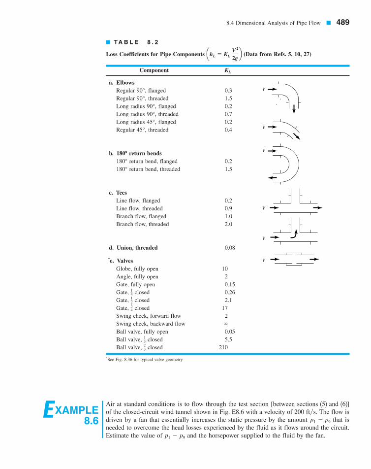
8.4 Dimensional Analysis of Pipe Flow � 489
� TA B L E 8 . 2
Loss Coefficients for Pipe Components (Data from Refs. 5, 10, 27)
Component
a. ElbowsRegular flanged 0.3Regular threaded 1.5Long radius flanged 0.2Long radius threaded 0.7Long radius flanged 0.2Regular threaded 0.4
b. return bendsreturn bend, flanged 0.2return bend, threaded 1.5
c. TeesLine flow, flanged 0.2Line flow, threaded 0.9Branch flow, flanged 1.0Branch flow, threaded 2.0
d. Union, threaded 0.08
*e. ValvesGlobe, fully open 10Angle, fully open 2Gate, fully open 0.15Gate, closed 0.26Gate, closed 2.1Gate, closed 17Swing check, forward flow 2Swing check, backward flow �
Ball valve, fully open 0.05Ball valve, closed 5.5Ball valve, closed 210
*See Fig. 8.36 for typical valve geometry
23
13
34
12
14
180°180°180�
45°,45°,90°,90°,
90°,90°,
KL
ahL � KL V 2
2gb
V
V
V
V
V
V
EXAMPLE8.6
Air at standard conditions is to flow through the test section [between sections 152 and 162]of the closed-circuit wind tunnel shown in Fig. E8.6 with a velocity of 200 ft�s. The flow isdriven by a fan that essentially increases the static pressure by the amount that isneeded to overcome the head losses experienced by the fluid as it flows around the circuit.Estimate the value of and the horsepower supplied to the fluid by the fan.p1 � p9
p1 � p9
7708d_c08_442-531 7/23/01 2:40 PM Page 489

490 � Chapter 8 / Viscous Flow in Pipes
SOLUTION
The maximum velocity within the wind tunnel occurs in the test section 1smallest area2. Thus,the maximum Mach number of the flow is where and fromEq. 1.20 the speed of sound is
Thus, As was indicated in Chapter 3 and discussedfully in Chapter 11, most flows can be considered as incompressible if the Mach number isless than about 0.3. Hence, we can use the incompressible formulas for this problem.
The purpose of the fan in the wind tunnel is to provide the necessary energy to over-come the net head loss experienced by the air as it flows around the circuit. This can befound from the energy equation between points 112 and 192 as
where is the total head loss from 112 to 192. With and this gives
(1)
Similarly, by writing the energy equation 1Eq. 5.842 across the fan, from 192 to 112, we obtain
where is the actual head rise supplied by the pump 1fan2 to the air. Again since and this, when combined with Eq. 1, becomes
The actual power supplied to the air 1horsepower, 2 is obtained from the fan head by
(2)
Thus, the power that the fan must supply to the air depends on the head loss associ-ated with the flow through the wind tunnel. To obtain a reasonable, approximate answer wemake the following assumptions. We treat each of the four turning corners as a mitered bendwith guide vanes so that from Fig. 8.31 Thus, for each corner
where, because the flow is assumed incompressible, The values of A and thecorresponding velocities throughout the tunnel are given in Table E8.6.
V � V5A5�A.
hLcorner� KL
V 2
2g� 0.2
V 2
2g
KLcorner� 0.2.
pa � gQhp � gA5V5hp � gA5V5hL1 – 9
pa
hp �1p1 � p92g
� hL1 – 9
V9 � V1
z9 � z1hp
p9
g�
V 29
2g� z9 � hp �
p1
g�
V 21
2g� z9
p1
g�
p9
g� hL1 – 9
V1 � V9z1 � z9hL1 – 9
p1
g�
V 21
2g� z1 �
p9
g�
V 29
2g� z9 � hL1 – 9
Ma5 � 200�1117 � 0.179.� 1117 ft�s.c5 � 1kRT521�2 � 51.411716 ft # lb�slug # °R2 3 1460 � 592°R 4 61�2
V5 � 200 ft�sMa5 � V5 �c5,
Q
Flow-straighteningscreens
(5) (6)
(7)
(8)
(9)(1)(2)
(3)
(4)
Fan
Testsection
V5 = 200 ft/s
Location Area ( ) Velocity ( )
1 22.0 36.42 28.0 28.63 35.0 22.94 35.0 22.95 4.0 200.06 4.0 200.07 10.0 80.08 18.0 44.49 22.0 36.4
ft�sft2
� F I G U R E E 8 . 6
7708d_c08_442-531 7/23/01 2:40 PM Page 490

8.4 Dimensional Analysis of Pipe Flow � 491
We also treat the enlarging sections from the end of the test section 162 to the begin-ning of the nozzle 142 as a conical diffuser with a loss coefficient of This valueis larger than that of a well-designed diffuser 1see Fig. 8.29, for example2. Since the windtunnel diffuser is interrupted by the four turning corners and the fan, it may not be possibleto obtain a smaller value of for this situation. Thus,
The loss coefficients for the conical nozzle between section 142 and 152 and the flow-straightening screens are assumed to be and 1Ref. 132, respectively. Weneglect the head loss in the relatively short test section.
Thus, the total head loss is
or
or
Hence, from Eq. 1 we obtain the pressure rise across the fan as
(Ans)
From Eq. 2 we obtain the power added to the fluid as
or
(Ans)
With a closed-return wind tunnel of this type, all of the power required to maintain theflow is dissipated through viscous effects, with the energy remaining within the closed tun-nel. If heat transfer across the tunnel walls is negligible, the air temperature within the tun-nel will increase in time. For steady state operations of such tunnels, it is often necessary toprovide some means of cooling to maintain the temperature at acceptable levels.
It should be noted that the actual size of the motor that powers the fan must be greaterthan the calculated 62.3 hp because the fan is not 100% efficient. The power calculated aboveis that needed by the fluid to overcome losses in the tunnel, excluding those in the fan. Ifthe fan were 60% efficient, it would require a shaft power of to run the fan. Determination of fan 1or pump2 efficiencies can be a complex problem thatdepends on the specific geometry of the fan. Introductory material about fan performance ispresented in Chapter 12; additional material can be found in various references 1Refs. 14,15, 16, for example2.
It should also be noted that the above results are only approximate. Clever, careful de-sign of the various components 1corners, diffuser, etc.2 may lead to improved 1i.e., lower2
p � 62.3 hp� 10.602 � 104 hp
pa �34,300 ft # lb�s
550 1ft # lb�s2�hp� 62.3 hp
pa � 10.0765 lb�ft32 14.0 ft22 1200 ft�s2 1560 ft2 � 34,300 ft # lb�s
� 42.8 lb�ft2 � 0.298 psi
p1 � p9 � ghL1 – 9� 10.0765 lb�ft32 1560 ft2
hL1 – 9� 560 ft
� 0.2120022 � 4.0122.922 4 ft2�s2� 32132.2 ft�s22 4 � 30.2180.02 � 44.42 � 28.62 � 22.922 � 0.6120022
hL1–9� 30.21V 2
7 � V 28 � V 2
2 � V 232 � 0.6V 2
6 � 0.2V 25 � 4.0V 2
4 4 �2g
hL1–9� hLcorner7
� hLcorner8� hLcorner2
� hLcorner3� hLdif
� hLnoz� hLscr
KLscr� 4.0KLnoz
� 0.2
hLdif� KLdif
V 2
6
2g� 0.6
V 26
2g
KLdif
KLdif� 0.6.
7708d_c08_442-531 7/23/01 2:40 PM Page 491
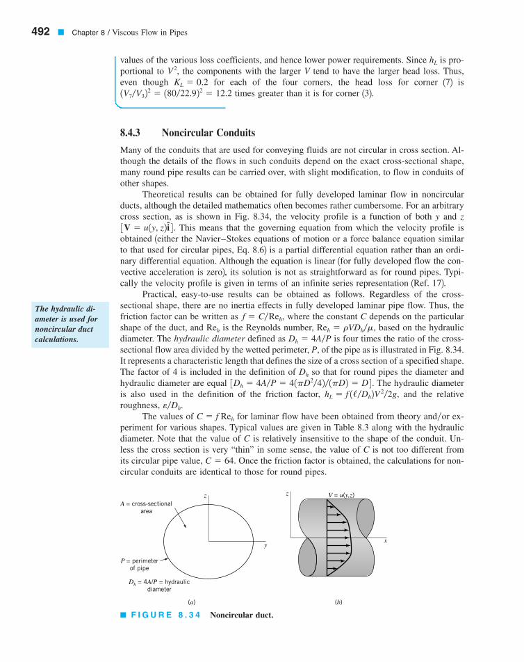
8.4.3 Noncircular Conduits
Many of the conduits that are used for conveying fluids are not circular in cross section. Al-though the details of the flows in such conduits depend on the exact cross-sectional shape,many round pipe results can be carried over, with slight modification, to flow in conduits ofother shapes.
Theoretical results can be obtained for fully developed laminar flow in noncircularducts, although the detailed mathematics often becomes rather cumbersome. For an arbitrarycross section, as is shown in Fig. 8.34, the velocity profile is a function of both y and z
This means that the governing equation from which the velocity profile isobtained 1either the Navier–Stokes equations of motion or a force balance equation similarto that used for circular pipes, Eq. 8.62 is a partial differential equation rather than an ordi-nary differential equation. Although the equation is linear 1for fully developed flow the con-vective acceleration is zero2, its solution is not as straightforward as for round pipes. Typi-cally the velocity profile is given in terms of an infinite series representation 1Ref. 172.
Practical, easy-to-use results can be obtained as follows. Regardless of the cross-sectional shape, there are no inertia effects in fully developed laminar pipe flow. Thus, thefriction factor can be written as where the constant C depends on the particularshape of the duct, and is the Reynolds number, based on the hydraulicdiameter. The hydraulic diameter defined as is four times the ratio of the cross-sectional flow area divided by the wetted perimeter, P, of the pipe as is illustrated in Fig. 8.34.It represents a characteristic length that defines the size of a cross section of a specified shape.The factor of 4 is included in the definition of so that for round pipes the diameter andhydraulic diameter are equal The hydraulic diameteris also used in the definition of the friction factor, and the relativeroughness,
The values of for laminar flow have been obtained from theory and�or ex-periment for various shapes. Typical values are given in Table 8.3 along with the hydraulicdiameter. Note that the value of C is relatively insensitive to the shape of the conduit. Un-less the cross section is very “thin” in some sense, the value of C is not too different fromits circular pipe value, Once the friction factor is obtained, the calculations for non-circular conduits are identical to those for round pipes.
C � 64.
C � f Reh
e�Dh.hL � f 1/�Dh2V 2�2g,
3Dh � 4A�P � 41pD2�42� 1pD2 � D 4 .Dh
Dh � 4A�PReh � rVDh�m,Reh
f � C�Reh,
3V � u1y, z2 i 4 .
492 � Chapter 8 / Viscous Flow in Pipes
values of the various loss coefficients, and hence lower power requirements. Since is pro-portional to the components with the larger V tend to have the larger head loss. Thus,even though for each of the four corners, the head loss for corner 172 is
times greater than it is for corner 132.1V7�V322 � 180�22.922 � 12.2KL � 0.2
V 2,hL
A = cross-sectionalarea
P = perimeterof pipe
Dh = 4A/P = hydraulicdiameter
(a) (b)
y
z
x
z V = u(y,z)
� F I G U R E 8 . 3 4 Noncircular duct.
The hydraulic di-ameter is used fornoncircular ductcalculations.
7708d_c08_442-531 7/23/01 2:40 PM Page 492

Calculations for fully developed turbulent flow in ducts of noncircular cross sectionare usually carried out by using the Moody chart data for round pipes with the diameter re-placed by the hydraulic diameter and the Reynolds number based on the hydraulic diameter.Such calculations are usually accurate to within about 15%. If greater accuracy is needed, amore detailed analysis based on the specific geometry of interest is needed.
8.4 Dimensional Analysis of Pipe Flow � 493
� TA B L E 8 . 3Friction Factors for Laminar Flow in Noncircular Ducts (Data from Ref. 18)
Shape Parameter
0.0001 71.80.01 80.10.1 89.40.6 95.61.00 96.0
a�b0 96.00.05 89.90.10 84.70.25 72.90.50 62.20.75 57.91.00 56.9
D1�D2
C � f Reh
EXAMPLE8.7
The Moody chart,developed for roundpipes, can also beused for noncircu-lar ducts.
D1
D2
Concentric AnnulusI.Dh = D2 – D1
a
b
Dh =2ab_____
a + b
RectangleII.
Air at a temperature of and standard pressure flows from a furnace through an 8-in.-diameter pipe with an average velocity of 10 ft�s. It then passes through a transition sectionand into a square duct whose side is of length a. The pipe and duct surfaces are smooth
Determine the duct size, a, if the head loss per foot is to be the same for the pipeand the duct.
SOLUTION
We first determine the head loss per foot for the pipe, and then size thesquare duct to give the same value. For the given pressure and temperature we obtain 1fromTable B.32 so that
With this Reynolds number and with we obtain the friction factor from Fig. 8.20as so that
Thus, for the square duct we must have
hL
/�
0.022
1 812 ft2
110 ft�s222132.2 ft�s22 � 0.0512
f � 0.022e�D � 0
Re �VDn
�110 ft�s2 1 8
12 ft21.89 � 10�4 ft2�s
� 35,300
n � 1.89 � 10�4 ft2�s
hL �/ � 1 f�D2 V 2�2g,
1e � 02.
120 °F
7708d_c08_442-531 7/23/01 2:40 PM Page 493
In the previous sections of this chapter, we discussed concepts concerning flow in pipes andducts. The purpose of this section is to apply these ideas to the solutions of various practi-cal problems. The application of the pertinent equations is straightforward, with rather sim-ple calculations that give answers to problems of engineering importance. The main idea in-volved is to apply the energy equation between appropriate locations within the flow system,with the head loss written in terms of the friction factor and the minor loss coefficients. Wewill consider two classes of pipe systems: those containing a single pipe 1whose length maybe interrupted by various components2, and those containing multiple pipes in parallel, se-ries, or network configurations.
494 � Chapter 8 / Viscous Flow in Pipes
(1)
where
(2)
is the velocity in the duct.By combining Eqs. 1 and 2 we obtain
or
(3)
where a is in feet. Similarly, the Reynolds number based on the hydraulic diameter is
(4)
We have three unknowns 1a, f, and Reh2 and three equations 1Eqs. 3, 4, and the third equa-tion in graphical form, Fig. 8.20, the Moody chart2. Thus, a trial and error solution is required.
As an initial attempt, assume the friction factor for the duct is the same as for the pipe.That is, assume From Eq. 3 we obtain while from Eq. 4 we have
From Fig. 8.20, with this Reynolds number and the given smooth duct weobtain which does not quite agree with the assumed value of f. Hence, we do nothave the solution. We try again, using the latest calculated value of as our guess.The calculations are repeated until the guessed value of f agrees with the value obtained fromFig. 8.20. The final result 1after only two iterations2 is and
(Ans)
Note that the length of the side of the equivalent square duct is or approximately 92% of the diameter of the equivalent duct. It can be shown that this value,92%, is a very good approximation for any pipe flow—laminar or turbulent. The cross-sectional area of the duct is greater than that of the round pipe
Also, it takes less material to form the round pipethan the square duct Circles are very efficient shapes.1perimeter � 4a � 29.4 in.2.25.1 in.2 1perimeter �pD �1A �pD2�4 � 50.3 in.22. 1A � a2 � 53.9 in.22
a�D � 7.34�8 � 0.918,
a � 0.611 ft � 7.34 in.
Reh � 3.03 � 104,f � 0.023,
f � 0.023f � 0.023,
Reh � 3.05 � 104.a � 0.606 ft,f � 0.022.
Reh �VsDh
n�13.49�a22a
1.89 � 10�4 �1.85 � 104
a
a � 1.30 f 1�5
0.0512 �f
a 13.49�a2222132.22
Vs �Q
A�
p
4 a 8
12 ftb2 110 ft�s2
a2 �3.49
a2
Dh � 4A�P � 4a2�4a � a and
hL
/�
f
Dh
V 2
s
2g� 0.0512
8.5 Pipe Flow Examples
Pipe systems maycontain a singlepipe with compo-nents or multipleinterconnectedpipes.
7708d_c08_442-531 7/23/01 2:40 PM Page 494
8.5.1 Single Pipes
The nature of the solution process for pipe flow problems can depend strongly on which ofthe various parameters are independent parameters 1the “given”2 and which is the dependentparameter 1the “determine”2. The three most common types of problems are shown in Table 8.4in terms of the parameters involved. We assume the pipe system is defined in terms of thelength of pipe sections used and the number of elbows, bends, and valves needed to conveythe fluid between the desired locations. In all instances we assume the fluid properties aregiven.
In a Type I problem we specify the desired flowrate or average velocity and determinethe necessary pressure difference or head loss. For example, if a flowrate of 2.0 gal�min isrequired for a dishwasher that is connected to the water heater by a given pipe system, whatpressure is needed in the water heater?
In a Type II problem we specify the applied driving pressure 1or, alternatively, the headloss2 and determine the flowrate. For example, how many gal�min of hot water are suppliedto the dishwasher if the pressure within the water heater is 60 psi and the pipe system de-tails 1length, diameter, roughness of the pipe; number of elbows; etc.2 are specified?
In a Type III problem we specify the pressure drop and the flowrate and determine thediameter of the pipe needed. For example, what diameter of pipe is needed between the wa-ter heater and dishwasher if the pressure in the water heater is 60 psi 1determined by the citywater system2 and the flowrate is to be not less than 2.0 gal�min 1determined by the manu-facturer2?
Several examples of these types of problems follow.
8.5 Pipe Flow Examples � 495
Pipe flow problemscan be categorizedby what parametersare given and whatis to be calculated.
� TA B L E 8 . 4Pipe Flow Types
Variable Type I Type II Type III
a. FluidDensity Given Given GivenViscosity Given Given Given
b. PipeDiameter Given Given DetermineLength Given Given GivenRoughness Given Given Given
c. FlowFlowrate or Average Given Determine GivenVelocity
d. PressurePressure Drop or Determine Given GivenHead Loss
7708d_c08_442-531 7/23/01 2:40 PM Page 495
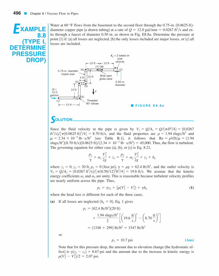
496 � Chapter 8 / Viscous Flow in Pipes
EXAMPLE8.8
(TYPE I,DETERMINEPRESSURE
DROP)
Water at flows from the basement to the second floor through the diameter copper pipe 1a drawn tubing2 at a rate of and ex-its through a faucet of diameter 0.50 in. as shown in Fig. E8.8a. Determine the pressure atpoint 112 if: 1a2 all losses are neglected, 1b2 the only losses included are major losses, or 1c2 alllosses are included.
Q � 12.0 gal�min � 0.0267 ft3�s0.75-in. 10.0625-ft2-60 °F
Q =12.0
gal/min
(1)
(2)
(3)
15 ft
10 ft
5 ft 10 ft
10 ft 10 ft(8)(7)
(6)
(4)
(5)
g
Threaded90° elbows
0.75-in. diametercopper pipe
Wide openglobe valve
0.50-in.diameter
KL = 2 based onpipe
velocity
� F I G U R E E 8 . 8 a
SOLUTION
Since the fluid velocity in the pipe is given by and the fluid properties are and1see Table B.12, it follows that
Thus, the flow is turbulent.The governing equation for either case 1a2, 1b2, or 1c2 is Eq. 8.21,
where and the outlet velocity isWe assume that the kinetic
energy coefficients and are unity. This is reasonable because turbulent velocity profilesare nearly uniform across the pipe. Thus,
(1)
where the head loss is different for each of the three cases.
(a) If all losses are neglected Eq. 1 gives
or
(Ans)
Note that for this pressure drop, the amount due to elevation change 1the hydrostatic ef-fect2 is and the amount due to the increase in kinetic energy isr1V 2
2 � V 212�2 � 2.07 psi.g1z2 � z12 � 8.67 psi
p1 � 10.7 psi
� 11248 � 2992 lb�ft2 � 1547 lb�ft2
�1.94 slugs�ft3
2 c a19.6
ftsb2
� a8.70 ftsb2 d
p1 � 162.4 lb�ft32 120 ft21hL � 02,
p1 � gz2 � 12r1V 2
2 � V 212 � ghL
a2a1
V2 � Q�A2 � 10.0267 ft3�s2� 3p10.50�1222ft2�4 4 � 19.6 ft�s.z1 � 0, z2 � 20 ft, p2 � 0 1free jet2, g � rg � 62.4 lb�ft3,
p1
g� a1
V 21
2g� z1 �
p2
g� a2
V 22
2g� z2 � hL
slugs�ft32 18.70 ft�s2 10.0625 ft2� 12.34 � 10�5 lb # s�ft22 � 45,000.Re � rVD�m � 11.94m � 2.34 � 10�5 lb # s�ft2r � 1.94 slugs�ft3ft3�s2� 3p10.0625 ft22�4 4 � 8.70 ft�s,
V1 � Q�A1 � Q� 1pD2�42 � 10.0267
7708d_c08_442-531 7/23/01 2:40 PM Page 496
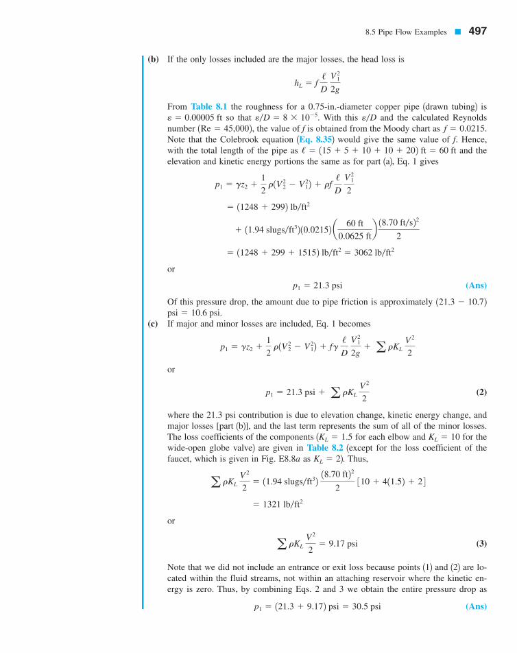
8.5 Pipe Flow Examples � 497
(b) If the only losses included are the major losses, the head loss is
From Table 8.1 the roughness for a 0.75-in.-diameter copper pipe 1drawn tubing2 isso that With this and the calculated Reynolds
number the value of f is obtained from the Moody chart as Note that the Colebrook equation 1Eq. 8.352 would give the same value of f. Hence,with the total length of the pipe as and theelevation and kinetic energy portions the same as for part 1a2, Eq. 1 gives
or
(Ans)
Of this pressure drop, the amount due to pipe friction is approximately
(c) If major and minor losses are included, Eq. 1 becomes
or
(2)
where the 21.3 psi contribution is due to elevation change, kinetic energy change, andmajor losses [part 1b2], and the last term represents the sum of all of the minor losses.The loss coefficients of the components 1 for each elbow and for thewide-open globe valve2 are given in Table 8.2 1except for the loss coefficient of thefaucet, which is given in Fig. E8.8a as 2. Thus,
or
(3)
Note that we did not include an entrance or exit loss because points 112 and 122 are lo-cated within the fluid streams, not within an attaching reservoir where the kinetic en-ergy is zero. Thus, by combining Eqs. 2 and 3 we obtain the entire pressure drop as
(Ans)p1 � 121.3 � 9.172 psi � 30.5 psi
a rKL V 2
2� 9.17 psi
� 1321 lb�ft2
a rKL V 2
2� 11.94 slugs�ft32 18.70 ft22
2 310 � 411.52 � 2 4
KL � 2
KL � 10KL � 1.5
p1 � 21.3 psi � a rKL V 2
2
p1 � gz2 �1
2 r1V 2
2 � V 212 � fg
/D
V 2
1
2g� a rKL
V 2
2
psi � 10.6 psi.121.3 � 10.72
p1 � 21.3 psi
� 11248 � 299 � 15152 lb�ft2 � 3062 lb�ft2
� 11.94 slugs�ft32 10.02152 a 60 ft
0.0625 ftb 18.70 ft�s22
2
� 11248 � 2992 lb�ft2
p1 � gz2 �1
2 r1V 2
2 � V 212 � rf
/D
V 2
1
2
/ � 115 � 5 � 10 � 10 � 202 ft � 60 ft
f � 0.0215.1Re � 45,0002, e�De�D � 8 � 10�5.e � 0.00005 ft
hL � f /D
V 1
2
2g
7708d_c08_442-531 7/23/01 2:40 PM Page 497
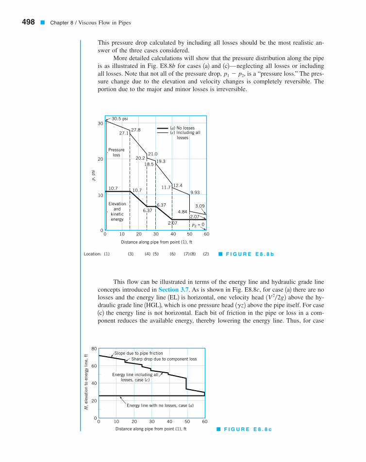
498 � Chapter 8 / Viscous Flow in Pipes
This pressure drop calculated by including all losses should be the most realistic an-swer of the three cases considered.
More detailed calculations will show that the pressure distribution along the pipeis as illustrated in Fig. E8.8b for cases 1a2 and 1c2—neglecting all losses or includingall losses. Note that not all of the pressure drop, is a “pressure loss.” The pres-sure change due to the elevation and velocity changes is completely reversible. The portion due to the major and minor losses is irreversible.
p1 � p2,
This flow can be illustrated in terms of the energy line and hydraulic grade lineconcepts introduced in Section 3.7. As is shown in Fig. E8.8c, for case 1a2 there are nolosses and the energy line 1EL2 is horizontal, one velocity head above the hy-draulic grade line 1HGL2, which is one pressure head above the pipe itself. For case1c2 the energy line is not horizontal. Each bit of friction in the pipe or loss in a com-ponent reduces the available energy, thereby lowering the energy line. Thus, for case
1gz21V 2�2g2
30
20
10
00 10 20 30 40 50 60
10.7 10.7
6.37
2.072.07
4.843.09
9.93
12.411.7
30.5 psi
27.127.8
20.221.0
18.519.3
(a) No losses(c) Including all
losses
Pressureloss
Elevationand
kineticenergy
p2 = 0
Distance along pipe from point (1), ft
p, p
si
Location: (1) (3) (4) (5) (6) (7) (8) (2)
6.37
80
60
40
20
00 10 20 30 40 50 60
Distance along pipe from point (1), ft
H, el
evat
ion
to e
nerg
y lin
e, f
t
Energy line with no losses, case (a)
Energy line including alllosses, case (c)
Sharp drop due to component lossSlope due to pipe friction
� F I G U R E E 8 . 8 b
� F I G U R E E 8 . 8 c
7708d_c08_498 8/16/01 5:11 PM Page 498
Although the governing pipe flow equations are quite simple, they can provide veryreasonable results for a variety of applications, as is shown in the next example.
8.5 Pipe Flow Examples � 499
1a2 the total head remains constant throughout the flow with a value of
For case 1c2 the energy line starts at
and falls to a final value of
The elevation of the energy line can be calculated at any point along the pipe. For ex-ample, at point 172, 50 ft from point 112,
The head loss per foot of pipe is the same all along the pipe. That is,
Thus, the energy line is a set of straight line segments of the same slope separated bysteps whose height equals the head loss of the minor component at that location. As isseen from Fig. E8.8c, the globe valve produces the largest of all the minor losses.
hL
/� f
V 2
2gD�
0.021518.70 ft�s222132.2 ft�s22 10.0625 ft2 � 0.404 ft�ft
H7 �p7
g�
V 27
2g� z7 �
19.93 � 1442 lb�ft2
162.4 lb�ft32 �18.70 ft�s22
2132.2 ft�s22 � 20 ft � 44.1 ft
H2 �p2
g�
V 22
2g� z2 � 0 �
119.6 ft�s222132.2 ft�s22 � 20 ft � 26.0 ft
H1 �p1
g�
V 21
2g� z1 �
130.5 � 1442lb�ft2
162.4 lb�ft32 �18.70 ft�s22
2132.2 ft�s22 � 0 � 71.6 ft
�p2
g�
V 22
2g� z2 �
p3
g�
V 33
2g� z3 � p
� 26.0 ft.
H � p1
g�
V 21
2g� z1 �
11547 lb�ft22162.4 lb�ft32 �
18.70 ft�s222132.2 ft�s22 � 0
EXAMPLE8.9
(TYPE I,DETERMINE
HEADLOSS)
Crude oil at with and 1about four times theviscosity of water2 is pumped across Alaska through the Alaskan pipeline, a 799-mile-long,4-ft-diameter steel pipe, at a maximum rate of million barrels�day or
Determine the horsepower needed for the pumps that drive this largesystem.
SOLUTION
From the energy equation 1Eq. 8.212 we obtain
where points 112 and 122 represent locations within the large holding tanks at either end ofthe line and is the head provided to the oil by the pumps. We assume that 1pumpedz1 � z2hp
p1
g�
V 21
2g� z1 � hp �
p2
g�
V 22
2g� z2 � hL
V � Q�A � 9.31 ft�s.� 117 ft3�s,Q � 2.4
m � 8 � 10�5 lb # s�ft2g � 53.7 lb�ft3140 °F
7708d_c08_442-531 7/23/01 2:40 PM Page 499
500 � Chapter 8 / Viscous Flow in Pipes
from sea level to sea level2, 1large, open tanks2 and Minor losses are negligible because of the large length-to-diameter ratio of
the relatively straight, uninterrupted pipe; Thus,
where from Fig. 8.20, since 1seeTable 8.12 and
Thus,
and the actual power supplied to the fluid, is
(Ans)
There are many reasons why it is not practical to drive this flow with a single pumpof this size. First, there are no pumps this large! Second, the pressure at the pump outletwould need to be No practical4-ft-diameter pipe would withstand this pressure. An equally unfeasible alternative would beto place the holding tank at the beginning of the pipe on top of a hill of height and let gravity force the oil through the 799-mi pipe!
To produce the desired flow, the actual system contains 12 pumping stations positionedat strategic locations along the pipeline. Each station contains four pumps, three of whichoperate at any one time 1the fourth is in reserve in case of emergency2. Each pump is driven by a 13,500-hp motor, thereby producing a total horsepower of stations 13 2 If we assume that the com-bination is approximately 60% efficient, there is a total of available to drive the fluid. This number compares favorably with the 202,000-hp answer cal-culated above.
The assumption of a oil temperature may not seem reasonable for flow acrossAlaska. Note, however, that the oil is warm when it is pumped from the ground and that the202,000 hp needed to pump the oil is dissipated as a head loss 1and therefore a temperaturerise2 along the pipe. However, if the oil temperature were rather than , the vis-cosity would be approximately 1twice as large2, but the friction factorwould only increase from at to at
This doubling of viscosity would result in only an 11% increasein power 1from 202,000 to 226,000 hp2. Because of the large Reynolds numbers involved,the shear stress is due mostly to the turbulent nature of the flow. That is, the value of Re forthis flow is large enough 1on the relatively flat part of the Moody chart2 so that f is nearlyindependent of Re 1or viscosity2.
70 °F 1Re � 3.88 � 1052. f � 0.0140140 °F 1Re � 7.76 � 1052f � 0.012516 � 10�5 lb # s�ft2
140 °F70 °F
140 °F
0.60 1486,0002 hp � 292,000 hppump�motor113,500 hp�pump2 � 486,000 hp.pump�stationp � 12
hL � 17,700 ft
p � ghL � 153.7 lb�ft32 117,700 ft2 11 ft2�144 in.22 � 6600 psi.
� 202,000 hp
� 1.11 � 108 ft # lb�s a 1 hp
550 ft # lb�sb
pa � gQhp � 153.7 lb�ft32 1117 ft3�s2 117,700 ft2pa,
hp � 0.012511.05 � 1062 19.31 ft�s222132.2 ft�s22 � 17,700 ft
7.76 � 105.19.31 ft�s2 14.0 ft2� 18 �10�5 lb # s�ft22 �Re � rVD�m� 3 153.7�32.22 slugs�ft3 4e�D � 10.00015 ft2� 14 ft2 � 0.0000375f � 0.0125
hp � hL � f /D
V 2
2g
1.05 � 106./�D � 1799 mi2 15280 ft�mi2� 14 ft2 �1 f/�D2V 2�2g2. hL �p1 � p2 � V1 � V2 � 0
Pipe flow problems in which it is desired to determine the flowrate for a given set ofconditions 1Type II problems2 often require trial-and-error solution techniques. This is be-
7708d_c08_442-531 7/23/01 2:40 PM Page 500

cause it is necessary to know the value of the friction factor to carry out the calculations, butthe friction factor is a function of the unknown velocity 1flowrate2 in terms of the Reynoldsnumber. The solution procedure is indicated in Example 8.10.
8.5 Pipe Flow Examples � 501
EXAMPLE8.10
(TYPE II,DETERMINEFLOWRATE)
According to an appliance manufacturer, the 4-in.-diameter galvanized iron vent on a clothesdryer is not to contain more than 20 ft of pipe and four elbows. Under these conditionsdetermine the air flowrate if the pressure within the dryer is 0.20 inches of water. Assume atemperature of and standard pressure.
SOLUTION
Application of the energy equation 1Eq. 8.212 between the inside of the dryer, point 112, andthe exit of the vent pipe, point 122, gives
(1)
where for the entrance is assumed to be 0.5 and that for each elbow is assumed to be 1.5.In addition we assume that and 1The change in elevation is often negligiblefor gas flows.2 Also, and or
Thus, with 1see Table B.32 and 1the air velocity in the pipe2, Eq. 1becomes
or
(2)
where V is in The value of f is dependent on Re, which is dependent on V, an unknown. However,
from Table B.3, and we obtain
or
(3)
where again V is in Also, since 1see Table 8.1 for the value of 2, we
know which particular curve of the Moody chart is pertinent to this flow. Thus, we have threerelationships 1Eqs. 2, 3, and the curve of Fig. 8.202 from which we can solvefor the three unknowns f, Re, and V. This is done easily by an iterative scheme as follows.
It is usually simplest to assume a value of f, calculate V from Eq. 2, calculate Re fromEq. 3, and look up the appropriate value of f in the Moody chart for this value of Re. If the
e�D � 0.0015
ee�D � 10.0005 ft2� 14�12 ft2 � 0.0015ft�s.
Re � 1860 V
Re �VDn
�1 412 ft2 V
1.79 � 10�4 ft2�s
n � 1.79 � 10�4 ft2�s
ft�s.
945 � 17.5 � 60f 2V 2
11.04 lb�ft2210.0709 lb�ft32 � c1 � f
120 ft21 412 ft2 � 0.5 � 411.52 d V 2
2132.2 ft�s22
V2 � Vg � 0.0709 lb�ft3
p1 � 10.2 in.2 a 1 ft
12 in.b 162.4 lb�ft32 � 1.04 lb�ft2
p1�gH2O � 0.2 in.,p2 � 0,z1 � z2.V1 � 0
KL
p1
g�
V 21
2g� z1 �
p2
g�
V 22
2g� z2 � f
/D
V 2
2g� a KL
V 2
2g
100 °F
90°
Some pipe flowproblems require atrial-and-error solu-tion technique.
7708d_c08_442-531 7/23/01 2:40 PM Page 501

502 � Chapter 8 / Viscous Flow in Pipes
assumed f and the new f do not agree, the assumed answer is not correct—we do not havethe solution to the three equations. Although values of either f, V, or Re could be assumed asstarting values, it is usually simplest to assume a value of f because the correct value oftenlies on the relatively flat portion of the Moody chart for which f is quite insensitive to Re.
Thus, we assume approximately the large Re limit for the given relativeroughness. From Eq. 2 we obtain
and from Eq. 3
With this Re and Fig. 8.20 gives which is not equal to the assumed solution1although it is close!2. We try again, this time with the newly obtained value ofwhich gives and With these values, Fig. 8.20 giveswhich agrees with the assumed value. Thus, the solution is or
(Ans)
Note that the need for the iteration scheme is because one of the equations,is in graphical form 1the Moody chart2. If the dependence of f on Re and
is known in equation form, this graphical dependency is eliminated, and the solutiontechnique may be easier. Such is the case if the flow is laminar so that the friction factor issimply For turbulent flow, we can use the Colebrook equation rather than theMoody chart, although this will normally require an iterative scheme also because of thecomplexity of the equation. As is shown below, such a formulation is ideally suited for aniterative computer solution.
We keep Eqs. 2 and 3 and use the Colebrook equation 1Eq. 8.35, rather than the Moodychart2 with to give
(4)
From Eq. 2 we have which can be combined with Eq. 3 to give
(5)
The combination of Eqs. 4 and 5 provides a single equation for the determination of f
(6)
A simple iterative solution of this equation gives in agreement with the above so-lution which used the Moody chart. [This iterative solution using the Colebrook equation canbe done as follows: 1a2 assume a value of f, 1b2 calculate a new value by using the assumedvalue in the right-hand side of Eq. 6, 1c2 use this new f to recalculate another value of f, and1d2 repeat until the successive values agree.]
Note that unlike the Alaskan pipeline example 1Example 8.92 in which we assumed mi-nor losses are negligible, minor losses are of importance in this example because of the rel-atively small length-to-diameter ratio: The ratio of minor to majorlosses in this case is The elbows and entrance pro-duce considerably more loss than the pipe itself.
KL �1 f/�D2 � 6.5� 30.029 1602 4 � 3.74./�D � 20� 14�122 � 60.
f � 0.029,
11f� �2.0 log a4.05 � 10�4 � 4.39 � 10�5 B60 �
7.5
fb
Re �57,20017.5 � 60 f
V � 3945� 17.5 � 60 f 2 4 1�2,
11f� �2.0 log ae�D
3.7�
2.51
Re1fb � �2.0 log a4.05 � 10�4 �
2.51
Re1fb
e�D � 0.0015
f � 64�Re.
e�Df � f1Re, e�D2,
Q � AV �p
4 1 4
12 ft22110.1 ft�s2 � 0.881 ft3�s
V � 10.1 ft�s,f � 0.029,Re � 18,800.V � 10.1 ft�sf � 0.029,
f � 0.022f � 0.029,e�D,
Re � 1860110.42 � 19,300
V � c 945
7.5 � 6010.0222 d1�2
� 10.4 ft�s
f � 0.022,
7708d_c08_442-531 7/23/01 2:40 PM Page 502
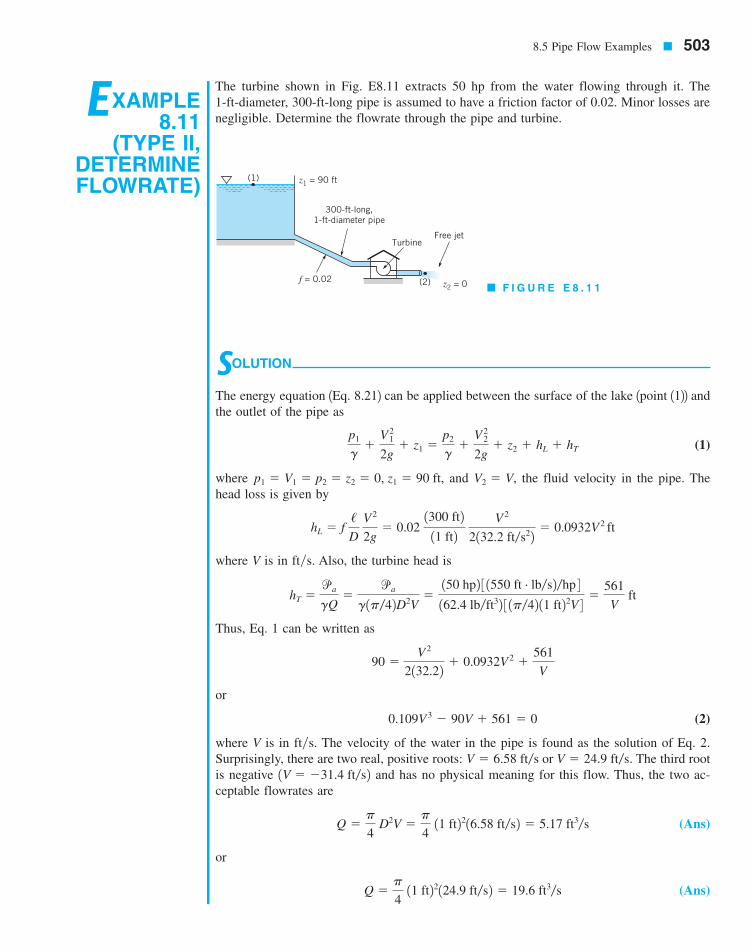
8.5 Pipe Flow Examples � 503
EXAMPLE8.11
(TYPE II,DETERMINEFLOWRATE)
The turbine shown in Fig. E8.11 extracts 50 hp from the water flowing through it. The 1-ft-diameter, 300-ft-long pipe is assumed to have a friction factor of 0.02. Minor losses arenegligible. Determine the flowrate through the pipe and turbine.
SOLUTION
The energy equation 1Eq. 8.212 can be applied between the surface of the lake 1point 1122 andthe outlet of the pipe as
(1)
where and the fluid velocity in the pipe. Thehead loss is given by
where V is in ft�s. Also, the turbine head is
Thus, Eq. 1 can be written as
or
(2)
where V is in ft�s. The velocity of the water in the pipe is found as the solution of Eq. 2.Surprisingly, there are two real, positive roots: The third rootis negative and has no physical meaning for this flow. Thus, the two ac-ceptable flowrates are
(Ans)
or
(Ans)Q �p
4 11 ft22124.9 ft�s2 � 19.6 ft3�s
Q �p
4 D2V �
p
4 11 ft2216.58 ft�s2 � 5.17 ft3�s
1V � �31.4 ft�s2V � 6.58 ft�s or V � 24.9 ft�s.
0.109V 3 � 90V � 561 � 0
90 �V 2
2132.22 � 0.0932V 2 �561
V
hT �pa
gQ�
pa
g1p�42D2V�150 hp2 3 1550 ft # lb�s2�hp 4162.4 lb�ft32 3 1p�42 11 ft22V 4 �
561
V ft
hL � f /D
V 2
2g� 0.02
1300 ft211 ft2
V 2
2132.2 ft�s22 � 0.0932V 2 ft
V2 � V,p1 � V1 � p2 � z2 � 0, z1 � 90 ft,
p1
g�
V 12
2g� z1 �
p2
g�
V 22
2g� z2 � hL � hT
(2)
Free jetTurbine
300-ft-long,1-ft-diameter pipe
(1)
f = 0.02 z2 = 0
z1 = 90 ft
� F I G U R E E 8 . 1 1
7708d_c08_442-531 7/23/01 2:40 PM Page 503

In pipe flow problems for which the diameter is the unknown 1Type III2, an iterative tech-nique is required. This is, again, because the friction factor is a function of the diameter—through both the Reynolds number and the relative roughness. Thus, neither
are known unless D is known. Examples 8.12 and 8.13 illustrate this.4rQ�pmD nor e�DRe � rVD�m �
504 � Chapter 8 / Viscous Flow in Pipes
Either of these two flowrates gives the same power, The reason for twopossible solutions can be seen from the following. With the low flowrate we obtain the head loss and turbine head as and Because of therelatively low velocity there is a relatively small head loss and, therefore, a large head availablefor the turbine. With the large flowrate we find and
The high-speed flow in the pipe produces a relatively large loss due to friction,leaving a relatively small head for the turbine. However, in either case the product of the tur-bine head times the flowrate is the same. That is, the power extracted is iden-tical for each case. Although either flowrate will allow the extraction of 50 hp from the wa-ter, the details of the design of the turbine itself will depend strongly on which flowrate isto be used. Such information can be found in Chapter 12 and various references about tur-bomachines 1Refs. 14, 19, 202.
If the friction factor were not given, the solution to the problem would be much morelengthy. A trial-and-error solution similar to that in Example 8.10 would be required alongwith the solution of a cubic equation.
1pa � gQhT2hT � 22.5 ft.
hL � 57.8 ft1Q � 19.6 ft3�s2,hT � 85.3 ft.hL � 4.04 ft
1Q � 5.17 ft3�s2,pa � gQhT.
EXAMPLE8.12
(TYPE IIIWITHOUT
MINORLOSSES,
DETERMINEDIAMETER)
Air at standard temperature and pressure flows through a horizontal, galvanized iron pipeat a rate of Determine the minimum pipe diameter if the pressure
drop is to be no more than 0.50 psi per 100 ft of pipe.
SOLUTION
We assume the flow to be incompressible with and Note that if the pipe were too long, the pressure drop from one end to the
other, would not be small relative to the pressure at the beginning, and compress-ible flow considerations would be required. For example, a pipe length of 200 ft gives
which is probablysmall enough to justify the incompressible assumption.
With and the energy equation 1Eq. 8.212 becomes
(1)
where or
where D is in feet. Thus, with and Eq. 1 / � 100 ft,p1 � p2 � 10.5 lb�in.22 1144 in.2�ft22V �
2.55
D2
V � Q�A � 4Q� 1pD22 � 412.0 ft3�s2�pD2,
p1 � p2 � f /D
rV 2
2
V1 � V2z1 � z2
3 10.50 psi2� 1100 ft2 4 1200 ft2�14.7 psi � 0.068 � 6.8%,1p1 � p22�p1 �
p1 � p2,10�7 lb # s�ft2.
m � 3.74 �r � 0.00238 slugs�ft3
2.0 ft3�s.1e � 0.0005 ft2
7708d_c08_442-531 7/23/01 2:40 PM Page 504
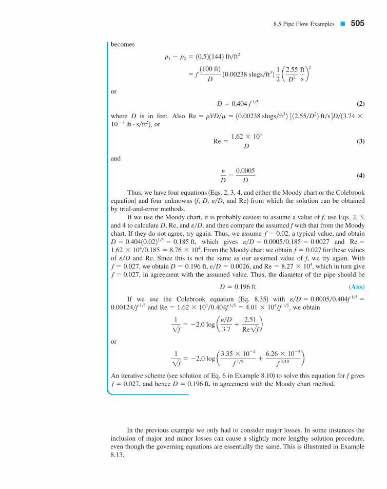
In the previous example we only had to consider major losses. In some instances theinclusion of major and minor losses can cause a slightly more lengthy solution procedure,even though the governing equations are essentially the same. This is illustrated in Example8.13.
8.5 Pipe Flow Examples � 505
becomes
or
(2)
where D is in feet. Also or
(3)
and
(4)
Thus, we have four equations 1Eqs. 2, 3, 4, and either the Moody chart or the Colebrookequation2 and four unknowns 1f, D, and Re2 from which the solution can be obtainedby trial-and-error methods.
If we use the Moody chart, it is probably easiest to assume a value of f, use Eqs. 2, 3,and 4 to calculate D, Re, and and then compare the assumed f with that from the Moodychart. If they do not agree, try again. Thus, we assume a typical value, and obtain
which gives and From the Moody chart we obtain for these values
of and Re. Since this is not the same as our assumed value of f, we try again. Withwe obtain and which in turn givein agreement with the assumed value. Thus, the diameter of the pipe should be
(Ans)
If we use the Colebrook equation 1Eq. 8.352 with and we obtain
or
An iterative scheme 1see solution of Eq. 6 in Example 8.102 to solve this equation for f givesand hence in agreement with the Moody chart method.D � 0.196 ft,f � 0.027,
11f� �2.0 log a3.35 � 10�4
f 1�5�
6.26 � 10�5
f 3�10 b
11f� �2.0 log ae�D
3.7�
2.51
Re1fb
Re � 1.62 � 104�0.404f 1�5 � 4.01 � 104�f 1�5,0.00124�f 1�5e�D � 0.0005�0.404f 1�5 �
D � 0.196 ft
f � 0.027,Re � 8.27 � 104,e�D � 0.0026,D � 0.196 ft,f � 0.027,
e�Df � 0.0271.62 � 104�0.185 � 8.76 � 104.
Re �e�D � 0.0005�0.185 � 0.0027D � 0.40410.0221�5 � 0.185 ft,f � 0.02,
e�D,
e�D,
e
D�
0.0005
D
Re �1.62 � 104
D
10�7 lb # s�ft22, Re � rVD�m � 10.00238 slugs�ft32 3 12.55�D22 ft�s 4D� 13.74 �
D � 0.404 f 1�5
� f 1100 ft2
D 10.00238 slugs�ft32 1
2 a2.55
D2 ftsb2
p1 � p2 � 10.52 11442 lb�ft2
7708d_c08_442-531 7/23/01 2:40 PM Page 505
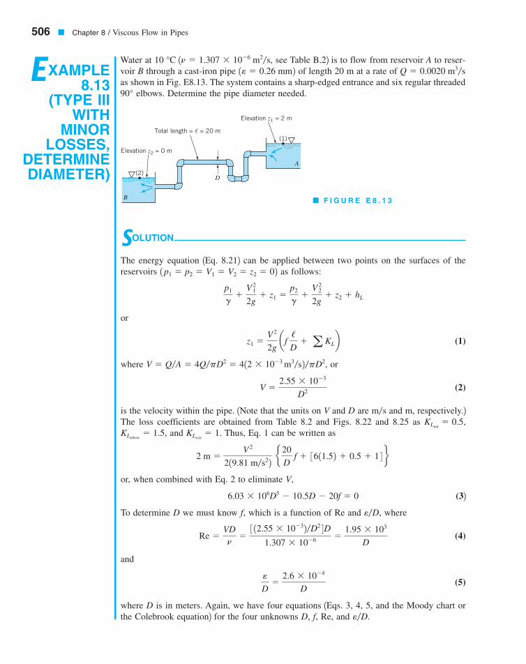
506 � Chapter 8 / Viscous Flow in Pipes
EXAMPLE8.13
(TYPE IIIWITH
MINORLOSSES,
DETERMINEDIAMETER) (2)
(1)
Elevation z2 = 0 m
Elevation z1 = 2 m
Total length = � = 20 m
D
B
A
� F I G U R E E 8 . 1 3
Water at 1 see Table B.22 is to flow from reservoir A to reser-voir B through a cast-iron pipe of length 20 m at a rate of as shown in Fig. E8.13. The system contains a sharp-edged entrance and six regular threaded
elbows. Determine the pipe diameter needed.90°
Q � 0.0020 m3�s1e � 0.26 mm2n � 1.307 � 10�6 m2�s,10 °C
SOLUTION
The energy equation 1Eq. 8.212 can be applied between two points on the surfaces of thereservoirs as follows:
or
(1)
where or
(2)
is the velocity within the pipe. 1Note that the units on V and D are and m, respectively.2The loss coefficients are obtained from Table 8.2 and Figs. 8.22 and 8.25 as
and Thus, Eq. 1 can be written as
or, when combined with Eq. 2 to eliminate V,
(32To determine D we must know f, which is a function of Re and where
(4)
and
(5)
where D is in meters. Again, we have four equations 1Eqs. 3, 4, 5, and the Moody chart orthe Colebrook equation2 for the four unknowns D, f, Re, and e�D.
e
D�
2.6 � 10�4
D
Re �VDn
�3 12.55 � 10�32�D2 4D
1.307 � 10�6 �1.95 � 103
D
e�D,
6.03 � 106D5 � 10.5D � 20f � 0
2 m �V 2
219.81 m�s22 e20
D f � 3611.52 � 0.5 � 1 4 f
KLexit� 1.KLelbow
� 1.5,KLent
� 0.5,m�s
V �2.55 � 10�3
D2
V � Q�A � 4Q�pD2 � 412 � 10�3 m3�s2�pD2,
z1 �V 2
2g af /
D� a
KLb
p1
g�
V 21
2g� z1 �
p2
g�
V 22
2g� z2 � hL
1p1 � p2 � V1 � V2 � z2 � 02
7708d_c08_442-531 7/23/01 2:40 PM Page 506

8.5.2 Multiple Pipe Systems
In many pipe systems there is more than one pipe involved. The complex system of tubes inour lungs 1beginning with the relatively large-diameter trachea and ending in minute bronchiafter numerous branchings2 and the maze of pipes in a city’s water distribution system aretypical of such systems. The governing mechanisms for the flow in multiple pipe systemsare the same as for the single pipe systems discussed in this chapter. However, because ofthe numerous unknowns involved, additional complexities may arise in solving for the flowin multiple pipe systems. Some of these complexities are discussed in this section.
The simplest multiple pipe systems can be classified into series or parallel flows, asare shown in Fig. 8.35. The nomenclature is similar to that used in electrical circuits. Indeed,an analogy between fluid and electrical circuits is often made as follows. In a simple elec-trical circuit, there is a balance between the voltage 1e2, current 1i2, and resistance 1R2 as givenby Ohm’s law: In a fluid circuit there is a balance between the pressure drop the flowrate or velocity 1Q or V 2, and the flow resistance as given in terms of the friction fac-tor and minor loss coefficients . For a simple flow it fol-lows that where a measure of the resistance to the flow, is proportional to f.R~,¢p � Q2R~,
3¢p � f 1/�D2 1rV 2�22 4 ,1 f and KL21¢p2,e � iR.
8.5 Pipe Flow Examples � 507
Consider the solution by using the Moody chart. Although it is often easiest to assumea value of f and make calculations to determine if the assumed value is the correct one, withthe inclusion of minor losses this may not be the simplest method. For example, if we as-sume and calculate D from Eq. 3, we would have to solve a fifth-order equation.With only major losses 1see Example 8.122, the term proportional to D in Eq. 3 is absent,and it is easy to solve for D if f is given. With both major and minor losses included 1repre-sented by the second and third terms in Eq. 32, this solution for D 1given f 2 would require atrial-and-error or iterative technique.
Thus, for this type of problem it is perhaps easier to assume a value of D, calculatethe corresponding f from Eq. 3, and with the values of Re and determined from Eqs. 4and 5, look up the value of f in the Moody chart 1or the Colebrook equation2. The solutionis obtained when the two values of f are in agreement. For example, assume sothat Eq. 3 gives and Eqs. 4 and 5 give and With these values of Reynolds number and relative roughness, the Moody chart gives
which does not coincide with that obtained from Eq. 3 Thus,
A few more rounds of calculation will reveal that the solution is given by with
(Ans)
It is interesting to attempt to solve this example if all losses are neglected so that Eq. 1becomes Clearly from Fig. E8.13, Obviously something is wrong. A fluidcannot flow from one elevation, beginning with zero pressure and velocity, and end up at alower elevation with zero pressure and velocity unless energy is removed 1i.e., a head loss ora turbine2 somewhere between the two locations. If the pipe is short 1negligible friction2 andthe minor losses are negligible, there is still the kinetic energy of the fluid as it leaves the pipeand enters the reservoir. After the fluid meanders around in the reservoir for some time, thiskinetic energy is lost and the fluid is stationary. No matter how small the viscosity is, the exitloss cannot be neglected. The same result can be seen if the energy equation is written fromthe free surface of the upstream tank to the exit plane of the pipe, at which point the kineticenergy is still available to the fluid. In either case the energy equation becomes in agreement with the inviscid results of Chapter 3 1the Bernoulli equation2. z1 � V 2�2g
z1 � 2 m.z1 � 0.
D � 45 mm
f � 0.032.D � 0.045 m
D � 0.05 m.1 f � 0.06802.f � 0.033,
e�D � 5.2 � 10�3.Re � 3.90 � 104f � 0.0680D � 0.05 m,
e�D
f � 0.02
An analogy be-tween pipe systemsand electrical cir-cuits can be made.
7708d_c08_442-531 7/23/01 2:40 PM Page 507

The main differences between the solution methods used to solve electrical circuit prob-lems and those for fluid circuit problems lie in the fact that Ohm’s law is a linear equation1doubling the voltage doubles the current2, while the fluid equations are generally nonlinear1doubling the pressure drop does not double the flowrate unless the flow is laminar2. Thus,although some of the standard electrical engineering methods can be carried over to helpsolve fluid mechanics problems, others cannot.
One of the simplest multiple pipe systems is that containing pipes in series, as is shownin Fig. 8.35a. Every fluid particle that passes through the system passes through each of thepipes. Thus, the flowrate 1but not the velocity2 is the same in each pipe, and the head lossfrom point A to point B is the sum of the head losses in each of the pipes. The governingequations can be written as follows:
and
where the subscripts refer to each of the pipes. In general, the friction factors will be differ-ent for each pipe because the Reynolds numbers and the relative rough-nesses will be different. If the flowrate is given, it is a straightforward calculation todetermine the head loss or pressure drop 1Type I problem2. If the pressure drop is given adthe flowerate is to be calculated 1Type II problem2, an iteration scheme is needed. In this sit-uation none of the friction factors, are known, so the calculations may involve more trial-and-error attempts than for corresponding single pipe systems. The same is true for prob-lems in which the pipe diameter 1or diameters2 is to be determined 1Type III problems2.
Another common multiple pipe system contains pipes in parallel, as is shown inFig. 8.35b. In this system a fluid particle traveling from A to B may take any of the pathsavailable, with the total flowrate equal to the sum of the flowrates in each pipe. However, bywriting the energy equation between points A and B it is found that the head loss experi-enced by any fluid particle traveling between these locations is the same, independent of thepath taken. Thus, the governing equations for parallel pipes are
Q � Q1 � Q2 � Q3
fi,
1ei�Di21Rei � rViDi�m2
hLA – B� hL1
� hL2� hL3
Q1 � Q2 � Q3
508 � Chapter 8 / Viscous Flow in Pipes
Q A V1(1) (2) (3)
V2D1 D2 D3 B
QV3
(a)
V1
V2
V3
D3
D2
D1
(1)
(2)
(3)
Q1
Q2
Q3
BA
(b)
� F I G U R E 8 . 3 5 Series (a) and parallel (b) pipe systems.
Series and parallelpipe systems are of-ten encountered.
7708d_c08_508 8/16/01 5:12 PM Page 508
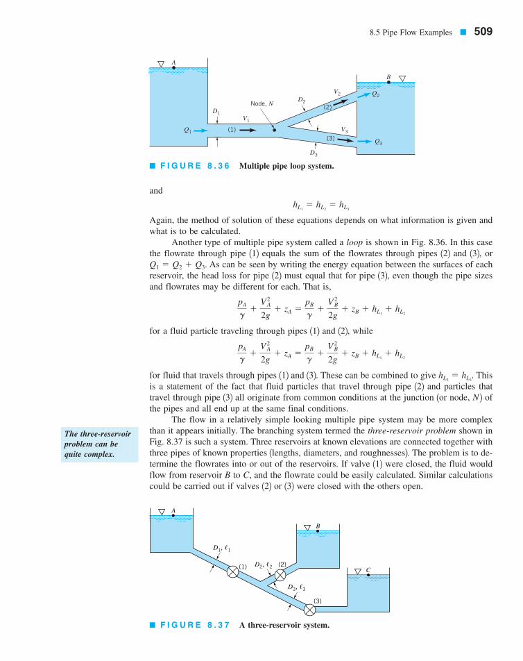
and
Again, the method of solution of these equations depends on what information is given andwhat is to be calculated.
Another type of multiple pipe system called a loop is shown in Fig. 8.36. In this casethe flowrate through pipe 112 equals the sum of the flowrates through pipes 122 and 132, or
As can be seen by writing the energy equation between the surfaces of eachreservoir, the head loss for pipe 122 must equal that for pipe 132, even though the pipe sizesand flowrates may be different for each. That is,
for a fluid particle traveling through pipes 112 and 122, while
for fluid that travels through pipes 112 and 132. These can be combined to give Thisis a statement of the fact that fluid particles that travel through pipe 122 and particles thattravel through pipe 132 all originate from common conditions at the junction 1or node, N 2 ofthe pipes and all end up at the same final conditions.
The flow in a relatively simple looking multiple pipe system may be more complexthan it appears initially. The branching system termed the three-reservoir problem shown inFig. 8.37 is such a system. Three reservoirs at known elevations are connected together withthree pipes of known properties 1lengths, diameters, and roughnesses2. The problem is to de-termine the flowrates into or out of the reservoirs. If valve 112 were closed, the fluid wouldflow from reservoir B to C, and the flowrate could be easily calculated. Similar calculationscould be carried out if valves 122 or 132 were closed with the others open.
hL2� hL3
.
pA
g�
V 2A
2g� zA �
pB
g�
V 2B
2g� zB � hL1
� hL3
pA
g�
V 2A
2g� zA �
pB
g�
V 2B
2g� zB � hL1
� hL2
Q1 � Q2 � Q3.
hL1� hL2
� hL3
8.5 Pipe Flow Examples � 509
B
A
(2)
(3)(1)
Node, N
Q3
Q2
Q1
D1
D2
D3
V1
V2
V3
A
B
C
(3)
(2)(1)
D1, �1
D2, �2
D3, �3
� F I G U R E 8 . 3 6 Multiple pipe loop system.
� F I G U R E 8 . 3 7 A three-reservoir system.
The three-reservoirproblem can bequite complex.
7708d_c08_442-531 7/23/01 2:40 PM Page 509

510 � Chapter 8 / Viscous Flow in Pipes
EXAMPLE8.14
Three reservoirs are connected by three pipes as are shown in Fig. E8.14. For simplicity weassume that the diameter of each pipe is 1 ft, the friction factor for each is 0.02, and becauseof the large length-to-diameter ratio, minor losses are negligible. Determine the flowrate intoor out of each reservoir.
With all valves open, however, it is not necessarily obvious which direction the fluidflows. For the conditions indicated in Fig. 8.37, it is clear that fluid flows from reservoir Abecause the other two reservoir levels are lower. Whether the fluid flows into or out of reser-voir B depends on the elevation of reservoirs B and C and the properties 1length, diameter,roughness2 of the three pipes. In general, the flow direction is not obvious, and the solutionprocess must include the determination of this direction. This is illustrated in Example 8.14.
SOLUTION
It is not obvious which direction the fluid flows in pipe 122. However, we assume that it flowsout of reservoir B, write the governing equations for this case, and check our assumption.The continuity equation requires that which, since the diameters are the samefor each pipe, becomes simply
(1)
The energy equation for the fluid that flows from A to C in pipes 112 and 132 can be writtenas
By using the fact that this becomes
For the given conditions of this problem we obtain
or
(2)322 � V 21 � 0.4V 2
3
100 ft �0.02
2132.2 ft�s22 1
11 ft2 3 11000 ft2V 21 � 1400 ft2V 2
3 4
zA � f1 /1
D1 V 2
1
2g� f3
/3
D3 V 2
3
2g
pA � pC � VA � VC � zC � 0,
pA
g�
V 2A
2g� zA �
pC
g�
V 2C
2g� zC � f1
/1
D1 V 2
1
2g� f3
/3
D3 V 2
3
2g
V1 � V2 � V3
Q1 � Q2 � Q3,
AElevation = 100 ft
Elevation =20 ft
Elevation =0 ft
(1)
(2)
(3)
D1 = 1 ft�1 = 1000 ft
D2 = 1 ft�2 = 500 ft
D3 = 1 ft�3 = 400 ft
C
B
� F I G U R E E 8 . 1 4
For some pipe sys-tems, the directionof flow is notknown a priori.
7708d_c08_442-531 7/23/01 2:40 PM Page 510

8.5 Pipe Flow Examples � 511
where and are in ft�s. Similarly the energy equation for fluid flowing from B and C is
or
For the given conditions this can be written as
(3)
Equations 1, 2, and 3 1in terms of the three unknowns and 2 are the governing equa-tions for this flow, provided the fluid flows from reservoir B. It turns out, however, that thereis no solution for these equations with positive, real values of the velocities. Although theseequations do not appear to be complicated, there is no simple way to solve them directly.Thus, a trial-and-error solution is suggested. This can be accomplished as follows. Assumea value of calculate from Eq. 2, and then from Eq. 3. It is found that the re-sulting trio does not satisfy Eq. 1 for any value of assumed. There is no solu-tion to Eqs. 1, 2, and 3 with real, positive values of and Thus, our original as-sumption of flow out of reservoir B must be incorrect.
To obtain the solution, assume the fluid flows into reservoirs B and C and out of A.For this case the continuity equation becomes
or
(4)
Application of the energy equation between points A and B and A and C gives
and
which, with the given data, become
(5)
and
(6)
Equations 4, 5, and 6 can be solved as follows. By substracting Eq. 5 from 6 we obtain
Thus, Eq. 5 can be written as
or
(7)
which, upon squaring both sides, can be written as
V 42 � 460 V 2
2 � 3748 � 0
2V22160 � 1.25V 22 � 98 � 2.75V 2
2
258 � 1V2 � V322 � 0.5V 22 � 1V2 � 2160 � 1.25V 2
222 � 0.5V 22
V3 � 2160 � 1.25V 22
322 � V 21 � 0.4 V 2
3
258 � V 21 � 0.5 V 2
2
zA � zC � f1 /1
D1 V 2
1
2g� f3
/3
D3 V 3
2
2g
zA � zB � f1 /1
D1 V 2
1
2g� f2
/2
D2 V 2
2
2g
V1 � V2 � V3
Q1 � Q2 � Q3
V3.V1, V2,V1V1, V2, V3
V2V3V1 7 0,
V3V1, V2,
64.4 � 0.5V 22 � 0.4V 2
3
zB � f2 /2
D2 V 2
2
2g� f3
/3
D3 V 2
3
2g
pB
g�
V 2B
2g� zB �
pC
g�
V 2C
2g� zC � f2
/2
D2 V 2
2
2g� f3
/3
D3 V 2
3
2g
V3V1
7708d_c08_442-531 7/23/01 2:40 PM Page 511
512 � Chapter 8 / Viscous Flow in Pipes
By using the quadratic formula we can solve for to obtain either Thus, either The value is not a root of theoriginal equations. It is an extra root introduced by squaring Eq. 7, which with becomes Thus, and from Eq. 5, The corre-sponding flowrates are
(Ans)
(Ans)
and
(Ans)
Note the slight differences in the governing equations depending on the direction of the flowin pipe 122—compare Eqs. 1, 2, and 3 with Eqs. 4, 5, and 6.
If the friction factors were not given, a trial-and-error procedure similar to that neededfor Type II problems 1see Section 8.5.12 would be required.
Q3 � Q1 � Q2 � 112.5 � 2.262 ft3�s � 10.2 ft3�s into C
� 2.26 ft3�s into B
Q2 � A2V2 �p
4 D2
2V2 �p
4 11 ft22 12.88 ft�s2
� 12.5 ft3�s from A
Q1 � A1V1 �p
4 D2
1V1 �p
4 11 ft22 115.9 ft�s2
V1 � 15.9 ft�s.V2 � 2.88 ft�s“1140 � �1140.”V2 � 21.3
V2 � 21.3 ft�sV2 � 21.3 ft�s or V2 � 2.88 ft�s.V 2
2 � 452 or V 22 � 8.30.V 2
2
The ultimate in multiple pipe systems is a network of pipes such as that shown inFig. 8.38. Networks like these often occur in city water distribution systems and other sys-tems that may have multiple “inlets” and “outlets.” The direction of flow in the various pipesis by no means obvious—in fact, it may vary in time, depending on how the system is usedfrom time to time.
The solution for pipe network problems is often carried out by use of node and loopequations similar in many ways to that done in electrical circuits. For example, the continu-ity equation requires that for each node 1the junction of two or more pipes2 the net flowrateis zero. What flows into a node must flow out at the same rate. In addition, the net pressuredifference completely around a loop 1starting at one location in a pipe and returning to thatlocation2 must be zero. By combining these ideas with the usual head loss and pipe flowequations, the flow throughout the entire network can be obtained. Of course, trial-and-errorsolutions are usually required because the direction of flow and the friction factors may notbe known. Such a solution procedure using matrix techniques is ideally suited for computeruse 1Refs. 21, 222.
� F I G U R E 8 . 3 8 A general pipenetwork.
Pipe network prob-lems can be solvedusing node andloop concepts.
7708d_c08_442-531 7/23/01 2:40 PM Page 512

It is often necessary to determine experimentally the flowrate in a pipe. In Chapter 3 we in-troduced various types of flow-measuring devices 1Venturi meter, nozzle meter, orifice me-ter, etc.2 and discussed their operation under the assumption that viscous effects were not im-portant. In this section we will indicate how to account for the ever-present viscous effectsin these flow meters. We will also indicate other types of commonly used flow meters.
8.6.1 Pipe Flowrate Meters
Three of the most common devices used to measure the instantaneous flowrate in pipes arethe orifice meter, the nozzle meter, and the Venturi meter. As was discussed in Section 3.6.3,each of these meters operates on the principle that a decrease in flow area in a pipe causesan increase in velocity that is accompanied by a decrease in pressure. Correlation of the pres-sure difference with the velocity provides a means of measuring the flowrate. In the absenceof viscous effects and under the assumption of a horizontal pipe, application of the Bernoulliequation 1Eq. 3.72 between points 112 and 122 shown in Fig. 8.39 gave
(8.37)
where Based on the results of the previous sections of this chapter, we antici-pate that there is a head loss between 112 and 122 so that the governing equations become
and
The ideal situation has and results in Eq. 8.37. The difficulty in including the headloss is that there is no accurate expression for it. The net result is that empirical coefficientsare used in the flowrate equations to account for the complex real world effects brought onby the nonzero viscosity. The coefficients are discussed below.
A typical orifice meter is constructed by inserting between two flanges of a pipe a flatplate with a hole, as shown in Fig. 8.40. The pressure at point 122 within the vena contractais less than that at point 112. Nonideal effects occur for two reasons. First, the vena contractaarea, is less than the area of the hole, by an unknown amount. Thus,where is the contraction coefficient Second, the swirling flow and turbulentmotion near the orifice plate introduce a head loss that cannot be calculated theoretically.Thus, an orifice discharge coefficient, is used to take these effects into account. That is,
(8.38)
where is the area of the hole in the orifice plate. The value of is a functionof and the Reynolds number where Typical values of CoV � Q�A1.Re � rVD�m,b � d�D
CoAo � pd 2�4
Q � CoQideal � Co Ao B21p1 � p22r11 � b42
Co,
1Cc 6 12.Cc
A2 � CcAo,Ao,A2,
hL � 0
p1
g�
V 21
2g�
p2
g�
V 22
2g� hL
Q � A1V1 � A2V2
b � D2�D1.
Qideal � A2V2 � A2 B21p1 � p22r11 � b42
8.6 Pipe Flowrate Measurement � 513
8.6 Pipe Flowrate Measurement
QD1
V1V2
D2
(1)(2)
� F I G U R E 8 . 3 9 Typicalpipe flow meter geometry.
An orifice dischargecoefficient is usedto account for non-ideal effects.
7708d_c08_442-531 7/23/01 2:40 PM Page 513

are given in Fig. 8.41. Note that the value of depends on the specific construction of theorifice meter 1i.e., the placement of the pressure taps, whether the orifice plate edge is squareor beveled, etc.2. Very precise conditions governing the construction of standard orifice me-ters have been established to provide the greatest accuracy possible 1Refs. 23, 242.
Another type of pipe flow meter that is based on the same principles used in the ori-fice meter is the nozzle meter, three variations of which are shown in Fig. 8.42. This deviceuses a contoured nozzle 1typically placed between flanges of pipe sections2 rather than a sim-ple 1and less expensive2 plate with a hole as in an orifice meter. The resulting flow patternfor the nozzle meter is closer to ideal than the orifice meter flow. There is only a slight venacontracta and the secondary flow separation is less severe, but there still are viscous effects.These are accounted for by use of the nozzle discharge coefficient, where
(8.39)
with As with the orifice meter, the value of is a function of the diameterratio, and the Reynolds number, Typical values obtained from ex-periments are shown in Fig. 8.43. Again, precise values of depend on the specific detailsof the nozzle design. Accepted standards have been adopted 1Ref. 242. Note that the nozzle meter is more efficient 1less energy dissipated2 than the orifice meter.
Cn 7 Co;Cn
Re � rVD�m.b � d�D,CnAn � pd 2�4.
Q � CnQideal � CnAn B21p1 � p22r11 � b42
Cn,
Co
514 � Chapter 8 / Viscous Flow in Pipes
Q
A1
A0(1) (2)A2
Pressure taps
dD1 = D
D2
d__D
= = 0.7β
0.5
0.6
0.40.2
D V
d
D D__2
0.66
0.64
0.62
0.60
0.58104 105 106 107 108
Re = VD/ρ µ
Co
� F I G U R E 8 . 4 0 Typicalorifice meter construction.
� F I G U R E 8 . 4 1 Orifice meter discharge coefficient (Ref. 24).
The nozzle meter ismore efficient thanthe orifice meter.
7708d_c08_442-531 7/23/01 2:40 PM Page 514
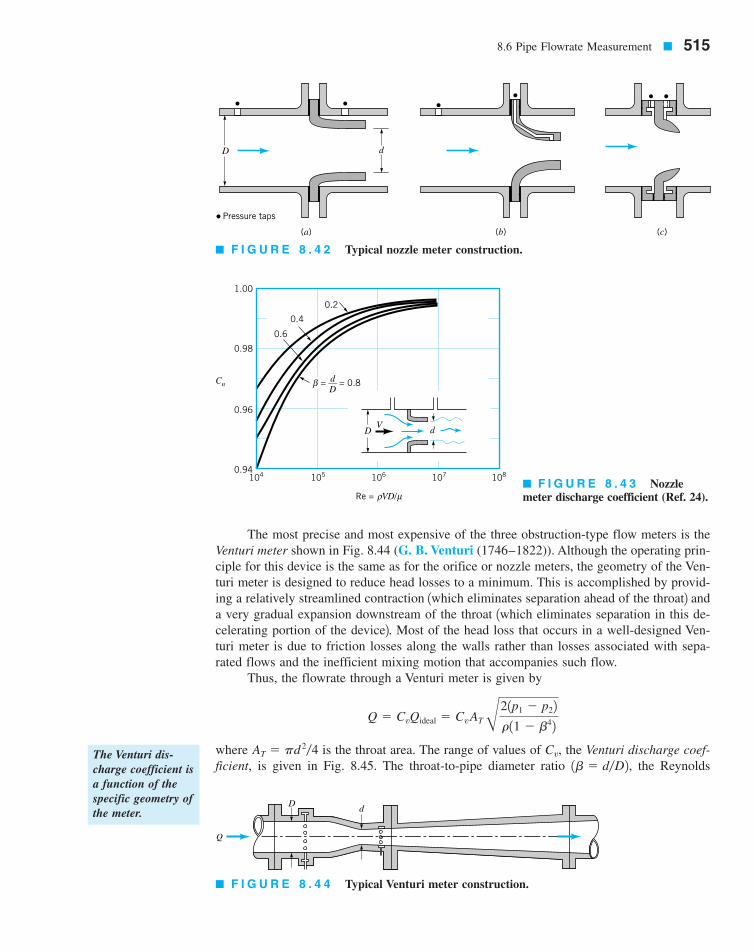
The most precise and most expensive of the three obstruction-type flow meters is theVenturi meter shown in Fig. 8.44 (G. B. Venturi (1746–1822)). Although the operating prin-ciple for this device is the same as for the orifice or nozzle meters, the geometry of the Ven-turi meter is designed to reduce head losses to a minimum. This is accomplished by provid-ing a relatively streamlined contraction 1which eliminates separation ahead of the throat2 anda very gradual expansion downstream of the throat 1which eliminates separation in this de-celerating portion of the device2. Most of the head loss that occurs in a well-designed Ven-turi meter is due to friction losses along the walls rather than losses associated with sepa-rated flows and the inefficient mixing motion that accompanies such flow.
Thus, the flowrate through a Venturi meter is given by
where is the throat area. The range of values of the Venturi discharge coef-ficient, is given in Fig. 8.45. The throat-to-pipe diameter ratio the Reynolds 1b � d�D2,
Cv,AT � pd 2�4
Q � CvQideal � CvAT B21p1 � p22r11 � b42
8.6 Pipe Flowrate Measurement � 515
Q
Dd
dD
(a) (b) (c)
Pressure taps
VD d
1.00
0.98
0.96
0.94104 105 106 107 108
Re = VD/ρ µ
Cn
0.6
0.4
0.2
= = 0.8d__D
β
� F I G U R E 8 . 4 4 Typical Venturi meter construction.
� F I G U R E 8 . 4 2 Typical nozzle meter construction.
� F I G U R E 8 . 4 3 Nozzle meter discharge coefficient (Ref. 24).
The Venturi dis-charge coefficient isa function of thespecific geometry ofthe meter.
7708d_c08_442-531 7/23/01 2:40 PM Page 515

number, and the shape of the converging and diverging sections of the meter are among theparameters that affect the value of
Again, the precise values of and depend on the specific geometry of the de-vices used. Considerable information concerning the design, use, and installation of standardflow meters can be found in various books 1Refs. 23, 24, 25, 26, 312.
CvCn, Co,Cv.
516 � Chapter 8 / Viscous Flow in Pipes
1.00
0.98
0.96
0.94104 105 106 107 108
Re = VD/ρ µ
CvRange of values
depending on specificgeometry
EXAMPLE8.15
Ethyl alcohol flows through a pipe of diameter in a refinery. The pressure dropacross the nozzle meter used to measure the flowrate is to be when the flowrateis Determine the diameter, d, of the nozzle.
SOLUTION
From Table 1.6 the properties of ethyl alcohol are and Thus,
From Eq. 8.39 the flowrate through the nozzle is
or
(1)
where d is in meters. Note that Equation 1 and Fig. 8.43 represent twoequations for the two unknowns d and that must be solved by trial and error.
As a first approximation we assume that the flow is ideal, or so that Eq. 1becomes
(2)
In addition, for many cases so that an approximate value of d can be obtainedfrom Eq. 2 as
d � 11.20 � 10�321�2 � 0.0346 m
1 � b4 � 1,
d � 11.20 � 10�3 21 � b421�2
Cn � 1.0,Cn
b � d�D � d�0.06.
1.20 � 10�3 �Cnd
221 � b4
Q � 0.003 m3�s � Cn p
4 d 2 B 214 � 103 N�m22
789 kg�m311 � b42
Re �rVDm
�4rQ
pDm�
41789 kg�m32 10.003 m3�s2p10.06 m2 11.19 � 10�3 N # s�m22 � 42,200
10�3 N # s�m2.m � 1.19 �r � 789 kg�m3
Q � 0.003 m3�s.¢p � 4.0 kPa
D � 60 mm
� F I G U R E 8 . 4 5 Venturimeter discharge coefficient (Ref. 23).
Precise standardsexist for the designof accurate flowmeters.
7708d_c08_442-531 7/23/01 2:40 PM Page 516
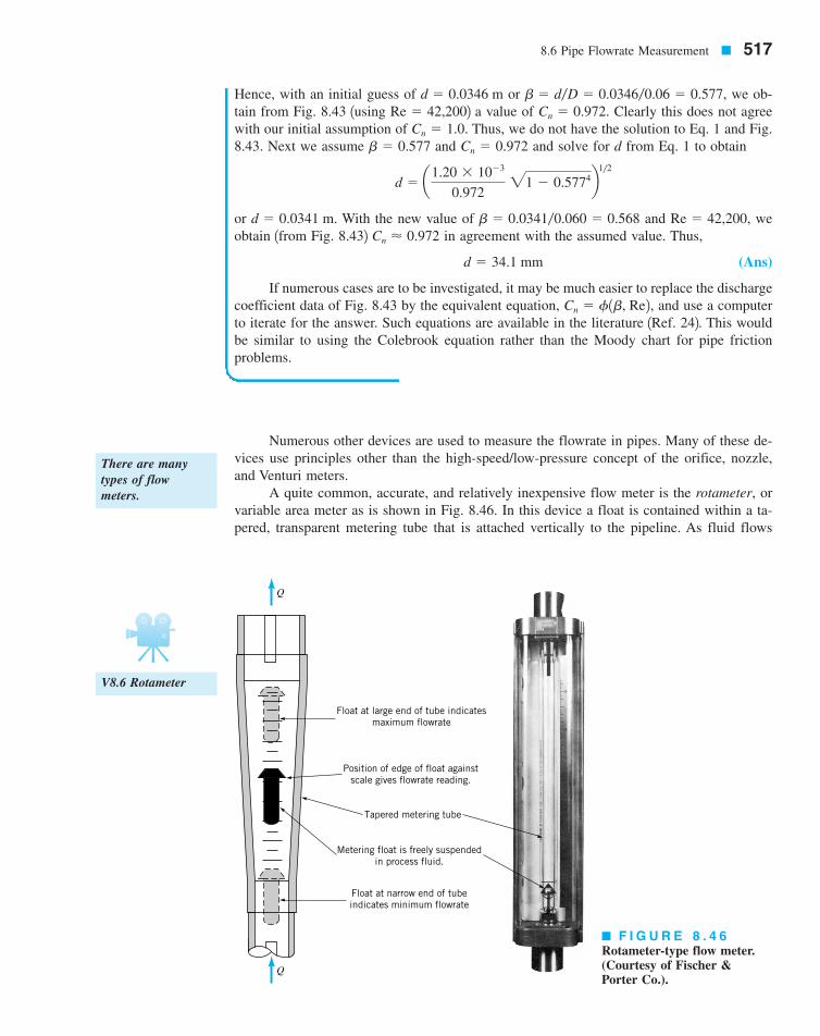
Numerous other devices are used to measure the flowrate in pipes. Many of these de-vices use principles other than the high-speed/low-pressure concept of the orifice, nozzle,and Venturi meters.
A quite common, accurate, and relatively inexpensive flow meter is the rotameter, orvariable area meter as is shown in Fig. 8.46. In this device a float is contained within a ta-pered, transparent metering tube that is attached vertically to the pipeline. As fluid flows
8.6 Pipe Flowrate Measurement � 517
Q
Q
Float at large end of tube indicatesmaximum flowrate
Position of edge of float againstscale gives flowrate reading.
Tapered metering tube
Metering float is freely suspendedin process fluid.
Float at narrow end of tubeindicates minimum flowrate
� F I G U R E 8 . 4 6Rotameter-type flow meter.(Courtesy of Fischer & Porter Co.).
Hence, with an initial guess of or we ob-tain from Fig. 8.43 1using 2 a value of Clearly this does not agreewith our initial assumption of Thus, we do not have the solution to Eq. 1 and Fig.8.43. Next we assume and and solve for d from Eq. 1 to obtain
or With the new value of and weobtain 1from Fig. 8.432 in agreement with the assumed value. Thus,
(Ans)
If numerous cases are to be investigated, it may be much easier to replace the dischargecoefficient data of Fig. 8.43 by the equivalent equation, and use a computerto iterate for the answer. Such equations are available in the literature 1Ref. 242. This wouldbe similar to using the Colebrook equation rather than the Moody chart for pipe frictionproblems.
Cn � f1b, Re2,d � 34.1 mm
Cn � 0.972Re � 42,200,b � 0.0341�0.060 � 0.568d � 0.0341 m.
d � a1.20 � 10�3
0.972 21 � 0.5774b1�2
Cn � 0.972b � 0.577Cn � 1.0.
Cn � 0.972.Re � 42,200b � d�D � 0.0346�0.06 � 0.577,d � 0.0346 m
There are manytypes of flow meters.
V8.6 Rotameter
7708d_c08_442-531 7/23/01 2:40 PM Page 517
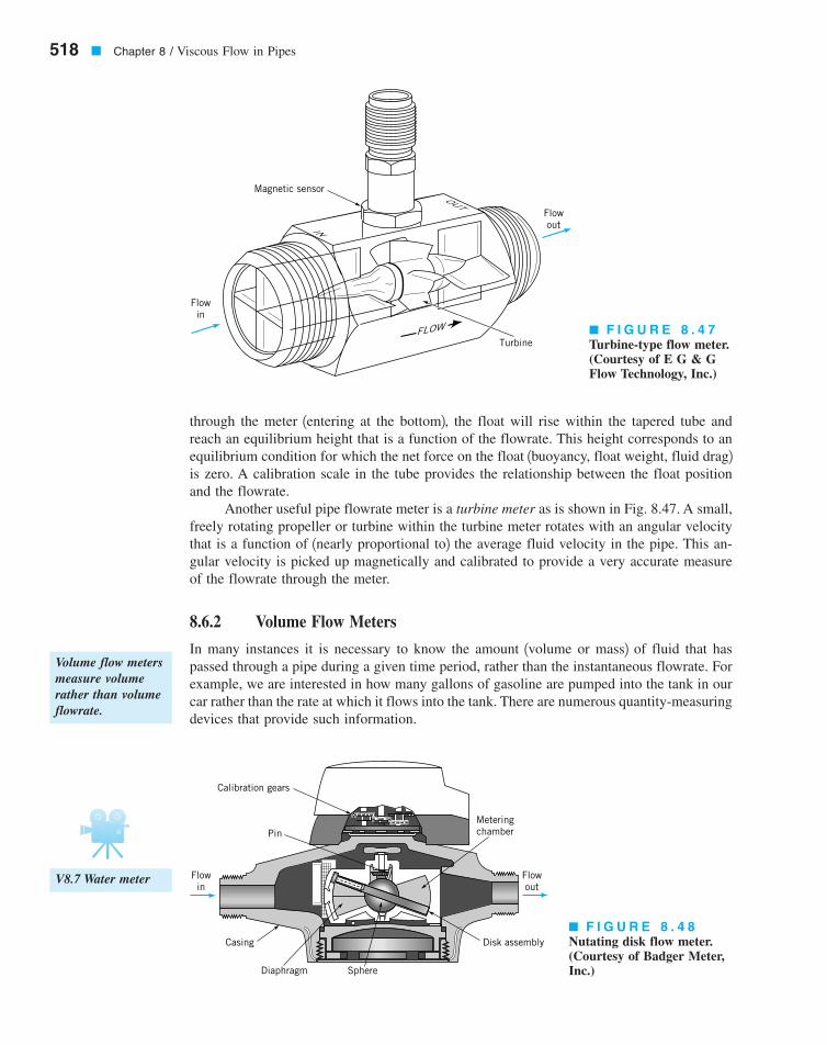
through the meter 1entering at the bottom2, the float will rise within the tapered tube andreach an equilibrium height that is a function of the flowrate. This height corresponds to anequilibrium condition for which the net force on the float 1buoyancy, float weight, fluid drag2is zero. A calibration scale in the tube provides the relationship between the float positionand the flowrate.
Another useful pipe flowrate meter is a turbine meter as is shown in Fig. 8.47. A small,freely rotating propeller or turbine within the turbine meter rotates with an angular velocitythat is a function of 1nearly proportional to2 the average fluid velocity in the pipe. This an-gular velocity is picked up magnetically and calibrated to provide a very accurate measureof the flowrate through the meter.
8.6.2 Volume Flow Meters
In many instances it is necessary to know the amount 1volume or mass2 of fluid that haspassed through a pipe during a given time period, rather than the instantaneous flowrate. Forexample, we are interested in how many gallons of gasoline are pumped into the tank in ourcar rather than the rate at which it flows into the tank. There are numerous quantity-measuringdevices that provide such information.
518 � Chapter 8 / Viscous Flow in Pipes
FLOW
IN
OUT
Magnetic sensor
Turbine
Flowin
Flowout
Calibration gears
Pin
Flowin
Flowout
Meteringchamber
Disk assembly
SphereDiaphragm
Casing
� F I G U R E 8 . 4 7Turbine-type flow meter.(Courtesy of E G & GFlow Technology, Inc.)
� F I G U R E 8 . 4 8Nutating disk flow meter.(Courtesy of Badger Meter,Inc.)
Volume flow metersmeasure volumerather than volumeflowrate.
V8.7 Water meter
7708d_c08_442-531 7/23/01 2:40 PM Page 518
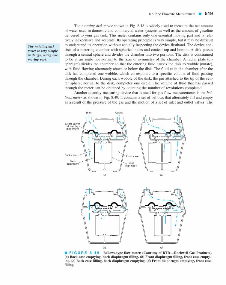
The nutating disk meter shown in Fig. 8.48 is widely used to measure the net amountof water used in domestic and commercial water systems as well as the amount of gasolinedelivered to your gas tank. This meter contains only one essential moving part and is rela-tively inexpensive and accurate. Its operating principle is very simple, but it may be difficultto understand its operation without actually inspecting the device firsthand. The device con-sists of a metering chamber with spherical sides and conical top and bottom. A disk passesthrough a central sphere and divides the chamber into two portions. The disk is constrainedto be at an angle not normal to the axis of symmetry of the chamber. A radial plate 1di-aphragm2 divides the chamber so that the entering fluid causes the disk to wobble 1nutate2,with fluid flowing alternately above or below the disk. The fluid exits the chamber after thedisk has completed one wobble, which corresponds to a specific volume of fluid passingthrough the chamber. During each wobble of the disk, the pin attached to the tip of the cen-ter sphere, normal to the disk, completes one circle. The volume of fluid that has passedthrough the meter can be obtained by counting the number of revolutions completed.
Another quantity-measuring device that is used for gas flow measurements is the bel-lows meter as shown in Fig. 8.49. It contains a set of bellows that alternately fill and emptyas a result of the pressure of the gas and the motion of a set of inlet and outlet valves. The
8.6 Pipe Flowrate Measurement � 519
Inlet Outlet
Slider valvesdriven by
diaphragm
Back case
Backdiaphragm
Front case
Frontdiaphragm
(a) (b)
(d)(c)
� F I G U R E 8 . 4 9 Bellows-type flow meter. (Courtesy of BTR—Rockwell Gas Products).(a) Back case emptying, back diaphragm filling. (b) Front diaphragm filling, front case empty-ing. (c) Back case filling, back diaphragm emptying. (d) Front diaphragm emptying, front casefilling.
The nutating diskmeter is very simplein design, using onemoving part.
7708d_c08_442-531 7/23/01 2:40 PM Page 519
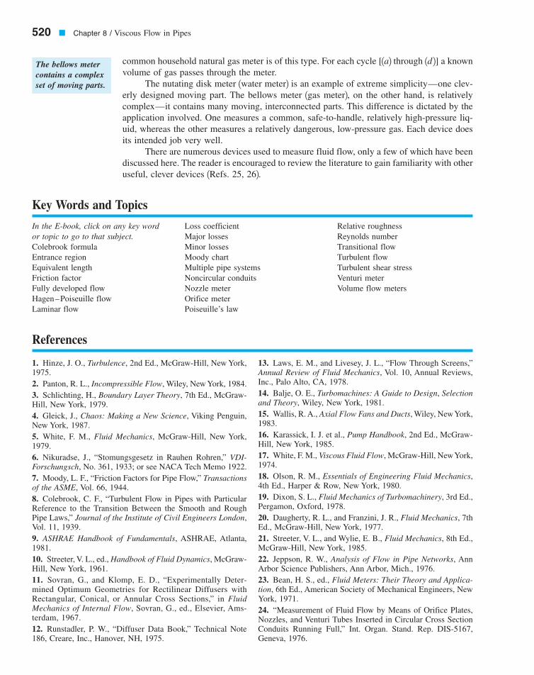
common household natural gas meter is of this type. For each cycle [1a2 through 1d 2] a knownvolume of gas passes through the meter.
The nutating disk meter 1water meter2 is an example of extreme simplicity—one clev-erly designed moving part. The bellows meter 1gas meter2, on the other hand, is relativelycomplex—it contains many moving, interconnected parts. This difference is dictated by theapplication involved. One measures a common, safe-to-handle, relatively high-pressure liq-uid, whereas the other measures a relatively dangerous, low-pressure gas. Each device doesits intended job very well.
There are numerous devices used to measure fluid flow, only a few of which have beendiscussed here. The reader is encouraged to review the literature to gain familiarity with otheruseful, clever devices 1Refs. 25, 262.
520 � Chapter 8 / Viscous Flow in Pipes
1. Hinze, J. O., Turbulence, 2nd Ed., McGraw-Hill, New York,1975.2. Panton, R. L., Incompressible Flow, Wiley, New York, 1984.3. Schlichting, H., Boundary Layer Theory, 7th Ed., McGraw-Hill, New York, 1979.4. Gleick, J., Chaos: Making a New Science, Viking Penguin,New York, 1987.5. White, F. M., Fluid Mechanics, McGraw-Hill, New York,1979.6. Nikuradse, J., “Stomungsgesetz in Rauhen Rohren,” VDI-Forschungsch, No. 361, 1933; or see NACA Tech Memo 1922.7. Moody, L. F., “Friction Factors for Pipe Flow,” Transactionsof the ASME, Vol. 66, 1944.8. Colebrook, C. F., “Turbulent Flow in Pipes with ParticularReference to the Transition Between the Smooth and RoughPipe Laws,” Journal of the Institute of Civil Engineers London,Vol. 11, 1939.9. ASHRAE Handbook of Fundamentals, ASHRAE, Atlanta,1981.10. Streeter, V. L., ed., Handbook of Fluid Dynamics, McGraw-Hill, New York, 1961.11. Sovran, G., and Klomp, E. D., “Experimentally Deter-mined Optimum Geometries for Rectilinear Diffusers withRectangular, Conical, or Annular Cross Sections,” in FluidMechanics of Internal Flow, Sovran, G., ed., Elsevier, Ams-terdam, 1967.12. Runstadler, P. W., “Diffuser Data Book,” Technical Note186, Creare, Inc., Hanover, NH, 1975.
13. Laws, E. M., and Livesey, J. L., “Flow Through Screens,”Annual Review of Fluid Mechanics, Vol. 10, Annual Reviews,Inc., Palo Alto, CA, 1978.14. Balje, O. E., Turbomachines: A Guide to Design, Selectionand Theory, Wiley, New York, 1981.15. Wallis, R. A., Axial Flow Fans and Ducts, Wiley, New York,1983.16. Karassick, I. J. et al., Pump Handbook, 2nd Ed., McGraw-Hill, New York, 1985.17. White, F. M., Viscous Fluid Flow, McGraw-Hill, New York,1974.18. Olson, R. M., Essentials of Engineering Fluid Mechanics,4th Ed., Harper & Row, New York, 1980.19. Dixon, S. L., Fluid Mechanics of Turbomachinery, 3rd Ed.,Pergamon, Oxford, 1978.20. Daugherty, R. L., and Franzini, J. R., Fluid Mechanics, 7thEd., McGraw-Hill, New York, 1977.21. Streeter, V. L., and Wylie, E. B., Fluid Mechanics, 8th Ed.,McGraw-Hill, New York, 1985.22. Jeppson, R. W., Analysis of Flow in Pipe Networks, AnnArbor Science Publishers, Ann Arbor, Mich., 1976.23. Bean, H. S., ed., Fluid Meters: Their Theory and Applica-tion, 6th Ed., American Society of Mechanical Engineers, NewYork, 1971.24. “Measurement of Fluid Flow by Means of Orifice Plates,Nozzles, and Venturi Tubes Inserted in Circular Cross SectionConduits Running Full,” Int. Organ. Stand. Rep. DIS-5167,Geneva, 1976.
References
Key Words and Topics
In the E-book, click on any key wordor topic to go to that subject.Colebrook formulaEntrance regionEquivalent lengthFriction factorFully developed flowHagen–Poiseuille flowLaminar flow
Loss coefficientMajor lossesMinor lossesMoody chartMultiple pipe systemsNoncircular conduitsNozzle meterOrifice meterPoiseuille’s law
Relative roughnessReynolds numberTransitional flowTurbulent flowTurbulent shear stressVenturi meterVolume flow meters
The bellows metercontains a complexset of moving parts.
7708d_c08_442-531 7/23/01 2:40 PM Page 520
Problems � 521
25. Goldstein, R. J., ed., Fluid Mechanics Measurements,Hemisphere Publishing, New York, 1983.26. Benedict, R. P., Measurement of Temperature, Pressure,and Flow, 2nd Ed., Wiley, New York, 1977.27. Hydraulic Institute, Engineering Data Book, 1st Ed., Cleve-land Hydraulic Institute, 1979.28. Harris, C. W., University of Washington Engineering Ex-perimental Station Bulletin, 48, 1928.29. Hamilton, J. B., University of Washington Engineering Ex-perimental Station Bulletin, 51, 1929.30. Miller, D. S., Internal Flow Systems, 2nd Ed., BHRA, Cran-field, UK, 1990.
31. Spitzer, D. W., ed., Flow Measurement: Practical Guidesfor Measurement and Control, Instrument Society of America,Research Triangle Park, North Carolina, 1991.32. Wilcox, D. C., Turbulence Modeling for CFD, DCW In-dustries, Inc., La Canada, California, 1994.33. Gleick, J., Chaos, Making a New Science, Penguin Books,New York, 1988.34. Mullin, T., ed., The Nature of Chaos, Oxford UniversityPress, Oxford, 1993.
In the E-book, click here to go to a set of review problems com-plete with answers and detailed solutions.
Review Problems
Problems
Note: Unless otherwise indicated use the values of fluid prop-erties found in the tables on the inside of the front cover. Prob-lems designated with an 1*2 are intended to be solved with theaid of a programmable calculator or a computer. Problems des-ignated with a 1 2 are “open-ended” problems and require crit-ical thinking in that to work them one must make various as-sumptions and provide the necessary data. There is not a uniqueanswer to these problems.
In the E-book, answers to the even-numbered problems canbe obtained by clicking on the problem number. In the E-book,access to the videos that accompany problems can be obtainedby clicking on the “video” segment (i.e., Video 8.3) of the prob-lem statement. The lab-type problems can be accessed by click-ing on the “click here” segment of the problem statement.
8.1 Rainwater runoff from a parking lot flows through a 3-ft-diameter pipe, completely filling it. Whether flow in a pipeis laminar or turbulent depends on the value of the Reynoldsnumber. (See Video V8.1.) Would you expect the flow to belaminar or turbulent? Support your answer with appropriate cal-culations.
† 8.2 Under normal circumstances is the air flow throughyour trachea 1your windpipe2 laminar or turbulent? List all as-sumptions and show all calculations.
8.3 The flow of water in a 3-mm-diameter pipe is to remainlaminar. Plot a graph of the maximum flowrate allowed as afunction of temperature for
8.4 Air at flows at standard atmospheric pressure ina pipe at a rate of 0.08 lb�s. Determine the maximum diame-ter allowed if the flow is to be turbulent.
8.5 Carbon dioxide at and a pressure of 550 kPa 1abs2flows in a pipe at a rate of 0.04 N�s. Determine the maximumdiameter allowed if the flow is to be turbulent.
8.6 It takes 20 seconds for a 0.5 cubic inch of water to flowthrough the 0.046-in. diameter tube of the capillary tube vis-
20 °C
100 °F
0 6 T 6 100 °C.
†
cometer shown in Video V1.3 and Fig. P8.6. Is the flow in thetube laminar or turbulent? Explain.
0.046 in.
� F I G U R E P 8 . 6
8.7 To cool a given room it is necessary to supply of air through an 8-in.-diameter pipe. Approximately how longis the entrance length in this pipe?
8.8 The wall shear stress in a fully developed flow portionof a 1.2-in.-diameter pipe carrying water is Deter-mine the pressure gradient, where x is in the flow di-rection, if the pipe is (a) horizontal, (b) vertical with flow up,or (c) vertical with flow down.
8.9 The pressure drop needed to force water through a hor-izontal l-in.-diameter pipe is 0.60 psi for every 12-ft length ofpipe. Determine the shear stress on the pipe wall. Determine
0p�0x,1.85 lb�ft2.
5 ft3�s
7708d_c08_442-531 8/30/01 7:10 AM Page 521 mac45 Mac 45:1st Shift:

522 � Chapter 8 / Viscous Flow in Pipes
the shear stress at distances 0.3 and 0.5 in. away from the pipewall.
8.10 Repeat Problem 8.9 if the pipe is on a hill. Is theflow up or down the hill? Explain.
8.11 Water flows in a constant diameter pipe with the fol-lowing conditions measured: At section 1a2 and
at section 1b2 and Is theflow from 1a2 to 1b2 or from 1b2 to 1a2? Explain.
8.12 Water flows downhill through a 3-in.-diameter steelpipe. The slope of the hill is such that for each mile (5280 ft)of horizontal distance, the change in elevation is Deter-mine the maximum value of if the flow is to remain lami-nar and the pressure all along the pipe is constant.
8.13 Some fluids behave as a non-Newtonian power-lawfluid characterized by where andso on, and C is a constant. 1If the fluid is the customaryNewtonian fluid.2 For flow in a round pipe of a diameter D,integrate the force balance equation 1Eq. 8.32 to obtain the ve-locity profile
*8.14 For the flow discussed in Problem 8.13, plot the di-mensionless velocity profile where is the centerline ve-locity 1at 2, as a function of the dimensionless radial co-ordinate where D is the pipe diameter. Consider valuesof and 7.
8.15 A fluid of density and viscosityflows steadily down a vertical 0.10-m-
diameter pipe and exits as a free jet from the lower end. De-termine the maximum pressure allowed in the pipe at a loca-tion 10 m above the pipe exit if the flow is to be laminar.
8.16 Water is pumped steadily from one large, open tankto another at the same elevation as shown in Fig. P8.16. De-termine the maximum power the pump can add to the water ifthe flow is to remain laminar.
m � 0.30 N � s�m2r � 1000 kg/m3
n � 1, 3, 5,r� 1D�22,r � 0
Vcu�Vc,
u1r2 ��n
1n � 12 a¢p
2/Cb1�n
c r 1n�12�n � aD
2b1n�12�n d
n � 1,n � 1, 3, 5,t � �C1du�dr2n,
¢z¢z ft.
zb � 68.2 ft.pb � 29.7 psiza � 56.8 ft;pa � 32.4 psi
20°
0.8 m�s. If the flow is laminar, determine the centerline veloc-ity and the flowrate.
8.20 Oil 1specific weight viscosityflows through a horizontal 23-mm-diameter tube as
shown in Fig. P8.20. A differential U-tube manometer is usedto measure the pressure drop along the tube. Determine therange of values for h for laminar flow.
N # s�m22 � 0.10� 8900 N�m3,
Length = 100 ftDiameter = 0.1 ft
P
� F I G U R E P 8 . 1 6
Q
SG = 7.0h
0.5 m
23 mmOil
� F I G U R E P 8 . 2 0
Q
SG = 0.87
4 m
20 mm
h
SG = 1.3
� F I G U R E P 8 . 2 28.17 Glycerin at flows upward in a vertical 75-mm-diameter pipe with a centerline velocity of 1.0 m�s. De-termine the head loss and pressure drop in a 10-m length of thepipe.
8.18 A fluid flows through a horizontal 0.1-in.-diameterpipe. When the Reynolds number is 1500, the head loss over a20-ft length of the pipe is 6.4 ft. Determine the fluid velocity.
8.19 A viscous fluid flows in a 0.10-m-diameter pipe suchthat its velocity measured 0.012 m away from the pipe wall is
20 °C
8.21 A fluid flows in a smooth pipe with a Reynolds num-ber of 6000. By what percent would the head loss be reducedif the flow could be maintained as laminar flow rather than theexpected turbulent flow?
8.22 Oil of and a kinematic viscosityflows through the vertical pipe shown in
Fig. P8.22 at a rate of Determine the manome-ter reading, h.
4 � 10�4 m3�s.m2�sn � 2.2 � 10�4
SG � 0.87
8.23 Determine the manometer reading, h, for Problem 8.22if the flow is up rather than down the pipe. Note: The manome-ter reading will be reversed.
8.24 For Problem 8.22, what flowrate 1magnitude and di-rection2 will cause
8.25 The kinetic energy coefficient, is defined inEq. 5.86. Show that its value for a power-law turbulent veloc-
a,
h � 0?
7708d_c08_442-531 7/23/01 2:40 PM Page 522

Problems � 523
ity profile 1Eq. 8.312 is given by
8.26 As shown in Video V8.3 and Fig. P8.26, the velocityprofile for laminar flow in a pipe is quite different from that forturbulent flow. With laminar flow the velocity profile is para-bolic; with turbulent flow at the velocity profilecan be approximated by the power-law profile shown in the fig-ure. (a) For laminar flow, determine at what radial location youwould place a Pitot tube if it is to measure the average veloc-ity in the pipe. (b) Repeat part (a) for turbulent flow withRe � 10,000.
Re � 10,000
34n41n � 32 12n � 32 4 .a � 1n � 12312n � 123�
1.0
0.5
0 0.5 1.0
r__R
r__R
u__Vc
u__Vc
Laminar with Re < 2100
= 1 – 2( )
r__R
u__Vc
Turbulent with Re = 10,000
= 1 – 1/5[ ]
R r
u
Vc
� F I G U R E P 8 . 2 6
Water
Air 0.108 in.
24 in.
h
� F I G U R E P 8 . 3 1
8.32 When soup is stirred in a bowl, there is considerableturbulence in the resulting motion (see Video V8.2). From avery simplistic standpoint, this turbulence consists of numerousintertwined swirls, each involving a characteristic diameter andvelocity. As time goes by, the smaller swirls (the fine scale struc-ture) die out relatively quickly, leaving the large swirls that con-tinue for quite some time. Explain why this is to be expected.
8.33 Determine the thickness of the viscous sublayer in asmooth 8-in.-diameter pipe if the Reynolds number is 25,000.
8.34 Water at flows through a 6-in.-diameter pipewith an average velocity of 15 ft�s. Approximately what is theheight of the largest roughness element allowed if this pipe isto be classified as smooth?
8.35 A 70-ft-long, 0.5-in.-diameter hose with a roughnessof ft is fastened to a water faucet where the pres-sure is Determine if there is no nozzle attached and theaverage velocity in the hose is Neglect minor losses andelevation changes.
8.36 Repeat Problem 8.35 if there is a nozzle of diameter0.25 in. attached to the end of the hose.
*8.37 The following equation is sometimes used in placeof the Colebrook equation 1Eq. 8.352:
for and 1Ref. 22, pg.2202. An advantage of this equation is that given Re and it does not require an iteration procedure to obtain f. Plot a graphof the percent difference in f as given by this equation and theoriginal Colebrook equation for Reynolds numbers in the rangeof validity of the above equation, with
8.38 Water flows at a rate of 10 gallons per minute in anew horizontal 0.75-in.-diameter galvanized iron pipe. Deter-mine the pressure gradient, along the pipe.
8.39 As shown in Fig. 8.3 and Video V8.1 (and quantifiedby Reynolds), the character of the flow within a pipe dependsstrongly on whether the flow is laminar or turbulent. One ad-vantage of laminar flow is that the friction factor and head lossare less than that for turbulent flow at the same Reynolds
¢p�/,
e�D � 10�4.
e�D,5000 6 Re 6 10�810�6 6 e�D 6 10�2
f �1.325
5ln 3 1e�3.7D2 � 15.74�Re0.92 4 62
6 ft�s.p1p1.
e � 0.0009
60 °F
8.27 Water at flows in a 6-in.-diameter pipe with aflowrate of 2.0 cfs. What is the approximate velocity at a dis-tance 2.0 in. away from the wall? Determine the centerlinevelocity.
8.28 During a heavy rainstorm, water from a parking lotcompletely fills an 18-in.-diameter, smooth, concrete stormsewer. If the flowrate is determine the pressure drop ina 100-ft horizontal section of the pipe. Repeat the problem ifthere is a 2-ft change in elevation of the pipe per 100 ft of itslength.
8.29 Carbon dioxide at a temperature of and a pres-sure of 600 kPa 1abs2 flows through a horizontal 40-mm-diam-eter pipe with an average velocity of 2 m�s. Determine the fric-tion factor if the pressure drop is per 10-m length ofpipe.
8.30 Water flows through a 6-in.-diameter horizontal pipeat a rate of 2.0 cfs and a pressure drop of 4.2 psi per 100 ft ofpipe. Determine the friction factor.
8.31 Air flows through the 0.108-in.-diameter, 24-in.-longtube shown in Fig. P8.31. Determine the friction factor if theflowrate is cfs when in. Compare yourresults with the expression Is the flow laminar orturbulent?
f � 64�Re.h � 1.70Q � 0.00191
235 N�m2
0 °C
10 ft3�s,
80 °F
7708d_c08_442-531 8/30/01 7:10 AM Page 523 mac45 Mac 45:1st Shift:

524 � Chapter 8 / Viscous Flow in Pipes
number. Under what circumstances might it be advantageous tohave turbulent rather than laminar pipe flow?
8.40 A garden hose is attached to a faucet that is fullyopened. Without a nozzle on the end of the hose, the water doesnot shoot very far. However, if you place your thumb over aportion of the end of the hose, it is possible to shoot the watera considerable distance. Explain this phenomenon. 1Note: Theflowrate decreases as the area covered by your thumb increases.2
8.41 Air at standard temperature and pressure flowsthrough a 1-in.-diameter galvanized iron pipe with an averagevelocity of 8 ft�s. What length of pipe produces a head lossequivalent to (a) a flanged elbow, (b) a wide-open anglevalve, or (c) a sharp-edged entrance?
*8.42 Water at flows through drawn tubings withdiameters of 0.025, 0.050, or 0.075 m. Plot the head loss ineach meter length of pipe for flowrates between and In your solution obtain the friction factorfrom the Colebrook formula.
8.43 Air at standard temperature and pressure flows at arate of 7.0 cfs through a horizontal, galvanized iron duct thathas a rectangular cross-sectional shape of 12 in. by 6 in. Esti-mate the pressure drop per 200 ft of duct.
8.44 Water flows at a rate of in an old, rusty 6-in.-diameter pipe that has a relative roughness of 0.010. It is pro-posed that by inserting a smooth plastic liner with an inside di-ameter of 5 in. into the old pipe as shown in Fig. P8.44, thepressure drop per mile can be reduced. Is it true that the linedpipe can carry the required at a lower pressure dropthan in the old pipe? Support your answer with appropriate cal-culations.
2.0 ft3/s
2.0 ft3/s
50 � 10�4 m3�s.5 � 10�4 m3�s
40 °C
90°8.47 Water flows at a rate of in a 0.12-m-diameter pipe that contains a sudden contraction to a 0.06-m-diameter pipe. Determine the pressure drop across the contrac-tion section. How much of this pressure difference is due tolosses and how much is due to kinetic energy changes?
8.48 A sign like the one shown in Fig. P8.48 is often at-tached to the side of a jet engine as a warning to airport work-ers. Based on Video V8.4 or Figs. 8.22 and 8.25, explain whythe danger areas (indicated in color) are the shape they are.
0.040 m3�s
6 in.
Old
5 in.
New
Liner
� F I G U R E P 8 . 4 4
C1130F
WARNING Stand clear ofHazard areas while engine is
running
WARNING Stand clear ofHazard areas while engine is
running
� F I G U R E P 8 . 4 8
Q
1__2
in.
(1)
Flow reducer washer
50 holes ofdiameter 0.05 in.
� F I G U R E P 8 . 4 6
† 8.45 Consider the process of donating blood. Bloodflows from a vein in which the pressure is greater than atmo-spheric, through a long small-diameter tube, and into a plasticbag that is essentially at atmospheric pressure. Based on fluidmechanics principles, estimate the amount of time it takes todonate a pint of blood. List all assumptions and show calcula-tions.
8.46 To conserve water and energy, a “flow reducer” isinstalled in the shower head as shown in Fig. P8.46. If the pres-sure at point 112 remains constant and all losses except for thatin the “flow reducer” are neglected, determine the value of theloss coefficient 1based on the velocity in the pipe2 of the “flowreducer” if its presence is to reduce the flowrate by a factor of2. Neglect gravity.
8.49 At time the level of water in tank A shown inFig. P8.49 is 2 ft above that in tank B. Plot the elevation of thewater in tank A as a function of time until the free surfaces inboth tanks are at the same elevation. Assume quasisteadyconditions—that is, the steady pipe flow equations are assumedvalid at any time, even though the flowrate does change 1slowly2in time. Neglect minor losses. Note: Verify and use the fact thatthe flow is laminar.
t � 0
7708d_c08_524 8/17/01 3:05 PM Page 524
Problems � 525
*8.50 Repeat Problem 8.49 if the pipe diameter is changedto 0.1 ft rather than 0.1 in. Note: The flow may not be laminarfor this case.
8.51 As shown in Fig. P8.51, water flows from one tank toanother through a short pipe whose length is n times the pipediameter. Head losses occur in the pipe and at the entrance andexit. (See Video V8.4.) Determine the maximum value of n ifthe major loss is to be no more than 10% of the minor loss andthe friction factor is 0.02.
3 ft 2 ft at t = 0
25 ft
0.1-in. diameter, galvanized iron
B A
3 ft
� F I G U R E P 8 . 4 9
D
� = nD
� F I G U R E P 8 . 5 1
Anglevalve
0.5 mh Tee
Surge chamber
Closed
D = 0.02 m
8 m5 m
(1)
� F I G U R E P 8 . 6 0
525 ftelevation
300-ft-long,0.4-ft-diameter
495 ftelevation
� F I G U R E P 8 . 6 2
duct with a flowrate of 8.2 cfs. Determine the pressure drop ininches of water per 200-ft length of duct.
8.58 Air flows through a rectangular galvanized iron ductof size 0.30 m by 0.15 m at a rate of Determine thehead loss in 12 m of this duct.
8.59 Air at standard conditions flows through a horizontal1 ft by 1.5 ft rectangular wooden duct at a rate of Determine the head loss, pressure drop, and power supplied bythe fan to overcome the flow resistance in 500 ft of the duct.
8.60 When the valve is closed, the pressure throughout thehorizontal pipe shown in Fig. P8.60 is 400 kPa, and the waterlevel in the closed, air-filled surge chamber is m. If thevalve is fully opened and the pressure at point 112 remains400 kPa, determine the new level of the water in the surge cham-ber. Assume the friction factor is and the fittings arethreaded fittings.
f � 0.02
h � 0.4
5000 ft3�min.
0.068 m3�s.
8.52 Gasoline flows in a smooth pipe of 40-mm diameterat a rate of If it were possible to prevent turbulencefrom occurring, what would be the ratio of the head loss for theactual turbulent flow compared to that if it were laminar flow?
8.53 A 3-ft-diameter duct is used to carry ventilating airinto a vehicular tunnel at a rate of Tests show thatthe pressure drop is 1.5 in. of water per 1500 ft of duct. Whatis the value of the friction factor for this duct and the approx-imate size of the equivalent roughness of the surface of the duct?
8.54 Natural gas 1 and 2 is pumped through a horizontal 6-in.-diameter cast-iron pipe at a rate of 800 lb�hr. If the pressure at section 112 is50 psi 1abs2, determine the pressure at section 122 8 mi down-stream if the flow is assumed incompressible. Is the incom-pressible assumption reasonable? Explain.
*8.55 Water flows in a 20-mm-diameter galvanized iron pipewith average velocities between 0.01 and 10.0 m�s. Plot the headloss per meter of pipe length over this velocity range. Discuss.
8.56 A fluid flows through a smooth horizontal 2-m-longtube of diameter 2 mm with an average velocity of 2.1 m�s.Determine the head loss and the pressure drop if the fluid is(a) air, (b) water, or (c) mercury.
8.57 Air at standard temperature and pressure flowsthrough a horizontal 2 ft by 1.3 ft rectangular galvanized iron
10�5 ft2�sn � 5.2 �r � 0.0044 slugs�ft3
9000 ft3�min.
0.001 m3�s.
8.61 What horsepower is added to water to pump it verticallythrough a 200-ft-long, 1.0-in.-diameter drawn tubing at a rate of
if the pressures at the inlet and outlet are the same?
8.62 Water flows from a lake as is shown in Fig. P8.62 ata rate of 4.0 cfs. Is the device inside the building a pump or aturbine? Explain and determine the horsepower of the device.Neglect all minor losses and assume the friction factor is 0.025.
0.060 ft3�s
8.63 Repeat Problem 8.62 if the flowrate is 1.0 cfs.
8.64 At a ski resort, water at is pumped through a 3-in.-diameter, 2000-ft-long steel pipe from a pond at an eleva-tion of 4286 ft to a snow-making machine at an elevation of 4623ft at a rate of If it is necessary to maintain a pressureof 180 psi at the snow-making machine, determine the horse-power added to the water by the pump. Neglect minor losses.
8.65 Water flows through the screen in the pipe shown inFig. P8.65 as indicated. Determine the loss coefficient for thescreen.
0.26 ft3�s.
40 °F
7708d_c08_442-531 7/23/01 2:40 PM Page 525

526 � Chapter 8 / Viscous Flow in Pipes
The pipes are 1-in. copper pipes with regular flanged fittings.The faucets are globe valves.
8.71 Water at flows through the coils of the heat ex-changer as shown in Fig. P8.71 at a rate of 0.9 gal�min. De-termine the pressure drop between the inlet and outlet of thehorizontal device.
40 °FV = 20 ft/s
Screen
Water
6 in.SG = 3.2
� F I G U R E P 8 . 6 5
6 in. length 6 in. length
4 in. length
Closed ballvalve
90° threadedelbows 0.60 in. dia.
Reducer Q = 0.020 cfs
1 in. length
Tee
� F I G U R E P 8 . 6 6
Q
18 in.
0.5-in. copper pipe (drawn tubing)
Threaded 180°return bend
� F I G U R E P 8 . 7 1
Q
Pump3-in. diameter,
f = 0.02
30 ft
10 ft
20 ft
Threadedelbow
� F I G U R E P 8 . 7 2
3 ft
L
D = 0.50 in.
Nozzle tip diameter = 0.30 in.Q =
0.010 cfs
10 ft�
Pump
Water
� F I G U R E P 8 . 7 3
8.66 Water flows steadily through the 0.75-in-diameter gal-vanized iron pipe system shown in Video V8.6 and Fig. P8.66at a rate of 0.020 cfs. Your boss suggests that friction losses inthe straight pipe sections are negligible compared to losses inthe threaded elbows and fittings of the system. Do you agreeor disagree with your boss? Support your answer with appro-priate calculations.
8.67 Because of a worn-out washer in a kitchen sink faucet,water drips at a steady rate even though the faucet is “turnedoff.” Readings from a water meter of the type shown in VideoV8.7 indicate that during a one-week time period when thehome owners were away, 200 gallons of water dripped from thefaucet. (a) If the pressure within the 0.50-in-diameter pipe is50 psi, determine the loss coefficient for the leaky faucet. (b)What length of the pipe would be needed to produce a headloss equivalent to the leaky faucet?
8.68 Assume a car’s exhaust system can be approximatedas 14 ft of 0.125-ft-diameter cast-iron pipe with the equivalentof six flanged elbows and a muffler. (See Video V8.5.) Themuffler acts as a resistor with a loss coefficient of Determine the pressure at the beginning of the exhaust systemif the flowrate is 0.10 cfs, the temperature is and theexhaust has the same properties as air.
8.69 Air is to flow through a smooth, horizontal, rectangu-lar duct at a rate of with a pressure drop of not morethan 40 mm of water per 50 m of duct. If the aspect ratio 1widthto height2 is 3 to 1, determine the size of the duct.
8.70 Repeat Problem 3.14 if all head losses are included.
100 m3�s
250 °F,
KL � 8.5.90°
8.72 Water at is pumped from a lake as shown inFig. P8.72. What is the maximum flowrate possible without cav-itation occurring?
40 °F
8.73 The -in.-diameter hose shown in Fig. P8.73 can with-stand a maximum pressure of 200 psi without rupturing. De-termine the maximum length, allowed if the friction factoris 0.022 and the flowrate is 0.010 cfs. Neglect minor losses.
/,
12
8.74 The hose shown in Fig. P8.73 will collapse if the pres-sure within it is lower than 10 psi below atmospheric pressure.Determine the maximum length, L, allowed if the friction fac-tor is 0.015 and the flowrate is 0.010 cfs. Neglect minor losses.
8.75 The pump shown in Fig. P8.75 delivers a head of 250 ftto the water. Determine the power that the pump adds to the wa-ter. The difference in elevation of the two ponds is 200 ft.
7708d_c08_526 8/16/01 5:14 PM Page 526

Problems � 527
4 in.
3 in.
(1)
� F I G U R E P 8 . 7 6
Intake manifold
MufflerExhaus
� F I G U R E P 8 . 8 0
(1)
Irrigationsystem:pipes, fittings,nozzles, etc.
WATERMETER
� F I G U R E P 8 . 8 4
Branch line (2) Mainline
6 ft
10 ft
All pipe is 6-in.-diameter plastic( /D = 0), flanged fittings∋
h
600 ftwith 15
90° elbows900 ft
� F I G U R E P 8 . 7 7
KLvalve = 5.0
KLelbow = 1.5
Pipe length = 500 ftPipe diameter = 0.75 ftPipe roughness = 0KLent
= 0.8
KLexit = 1.0
Pump
� F I G U R E P 8 . 7 5
Assume that the pressure drop through this system is whenthe engine is idling at 1000 rpm at a stop sign. Estimate thepressure drop (in terms of ) with the engine at 3000 rpmwhen you are driving on the highway. List all the assumptionsthat you made to arrive at your answer.
¢p1
¢p1
8.76 As shown in Video V8.6 and Fig. P8.76, water “bub-bles up” 3 in. above the exit of the vertical pipe attached tothree horizontal pipe segments. The total length of the 0.75-in.-diameter galvanized iron pipe between point (1) and the exit is21 in. Determine the pressure needed at point (1) to producethis flow.
8.77 The pressure at section 122 shown in Fig. P8.77 is notto fall below 60 psi when the flowrate from the tank varies from0 to 1.0 cfs and the branch line is shut off. Determine the mini-mum height, h, of the water tank under the assumption that (a) mi-nor losses are negligible, (b) minor losses are not negligible.
8.81 Water flows from a large open tank, through a 50-ft-long,0.10-ft-diameter pipe and exits with a velocity of when thewater level in the tank is 10 ft above the pipe exit. The sum of theminor loss coefficients for the pipe system is 12. Determine thenew water level needed in the tank if the velocity is to remain
when 20 ft of the pipe is removed (i.e., when the length isreduced to 30 ft). The minor loss coefficients remain the same.
8.82 Water is to flow at a rate of in a horizontalaluminum pipe The inlet and outlet pres-sures are 65 psi and 30 psi, respectively, and the pipe length is500 ft. Determine the diameter of this water pipe.
8.83 Water flows downward through a vertical smooth pipe.When the flowrate is there is no change in pressurealong the pipe. Determine the diameter of the pipe.
8.84 As shown in Fig. P8.84, a standard household watermeter is incorporated into a lawn irrigation system to measurethe volume of water applied to the lawn. Note that these me-ters measure volume, not volume flowrate. (See Video V8.7.)With an upstream pressure of the meter registeredthat of water was delivered to the lawn during an “on”cycle. Estimate the upstream pressure, needed if it is desiredto have delivered during an “on” cycle. List any as-sumptions needed to arrive at your answer.
150 ft3p1,
120 ft3p1 � 50 psi
0.5 ft3�s
1e � 5 � 10�6 ft2.3.5 ft3�s
5 ft/s
5 ft/s
8.85 When water flows from the tank shown in Fig. P8.85,the water depth in the tank as a function of time is as indicated.Determine the cross-sectional area of the tank. The total lengthof the 0.60-in.-diameter pipe is 20 ft, and the friction factor is0.03. The loss coefficients are: 0.50 for the entrance, 1.5 foreach elbow, and 10 for the valve.
8.78 Repeat Problem 8.77 with the assumption that thebranch line is open so that half of the flow from the tank goesinto the branch, and half continues in the main line.
8.79 Repeat Problem 3.43 if head losses are included.
8.80 The exhaust from your car’s engine flows through acomplex pipe system as shown in Fig. P8.80 and Video V8.5.
3 ftValve
h
2.0
1.5
1.00 100 200 300
t, s
h, f
t
� F I G U R E P 8 . 8 5
7708d_c08_527 8/16/01 5:15 PM Page 527

8.92 A fan is to produce a constant air speed of throughout the pipe loop shown in Fig. P8.92. The 3-m-diam-eter pipes are smooth, and each of the four 90-degree elbowshas a loss coefficient of 0.30. Determine the power that the fanadds to the air.
40 m/s
8.86 Water flows through a 2-in.-diameter pipe with a ve-locity of as shown in Fig. P8.86. The relative roughnessof the pipe is 0.004, and the loss coefficient for the exit is 1.0.Determine the height, h, to which the water rises in the piezome-ter tube.
15 ft/s
528 � Chapter 8 / Viscous Flow in Pipes
8.89 The pump shown in Fig. P8.89 adds 25 kW to the wa-ter and causes a flowrate of Determine the flowrateexpected if the pump is removed from the system. Assume
for either case and neglect minor losses.f � 0.016
0.04 m3�s.
F
V
Free jet
f = 0.020 Pipe weighs0.20 lb/ft
Bellows
D = 0.40 ft
� F I G U R E P 8 . 8 8
8 ft
8 ft
2 in.15 ft/s
h
Open
� F I G U R E P 8 . 8 6
40-mm-diameternozzle
60-mm-diameter,30-m-long pipe;
f = 0.016
Pump
� F I G U R E P 8 . 8 9
120 m of 0.30-m-diametercast iron pipe
1 m
20 mDiffuser
T
� F I G U R E P 8 . 9 1
Fan
V = 40 m/s
D = 3 m10 m
20 m
� F I G U R E P 8 . 9 2
20 m Bolts FilterFree jet
50 m 75 m
� F I G U R E P 8 . 8 7
8.87 Water flows from a large tank that sits on frictionlesswheels as shown in Fig. P8.87. The pipe has a diameter of 0.50m and a roughness of The loss coefficient forthe filter is 8; other minor losses are negligible. The tank andthe first 50-m section of the pipe are bolted to the last 75-msection of the pipe which is clamped firmly to the floor. De-termine the tension in the bolts.
9.2 � 10�5 m.
8.88 Water flows through two sections of the vertical pipeshown in Fig. P8.88. The bellows connection cannot support anyforce in the vertical direction. The 0.4-ft-diameter pipe weighs0.2 lb�ft, and the friction factor is assumed to be 0.02. At whatvelocity will the force, F, required to hold the pipe be zero?
8.90 A certain process requires 2.3 cfs of water to be de-livered at a pressure of 30 psi. This water comes from a largediameter supply main in which the pressure remains at 60 psi.If the galvanized iron pipe connecting the two locations is 200ft long and contains six threaded elbows, determine the pipediameter. Elevation differences are negligible.
8.91 The turbine shown in Fig. P8.91 develops 400 kW.Determine the flowrate if (a) head losses are negligible or(b) head loss due to friction in the pipe is considered. Assume
Note: There may be more than one solution or theremay be no solution to this problem.f � 0.02.
90°
7708d_c08_528 8/16/01 5:15 PM Page 528
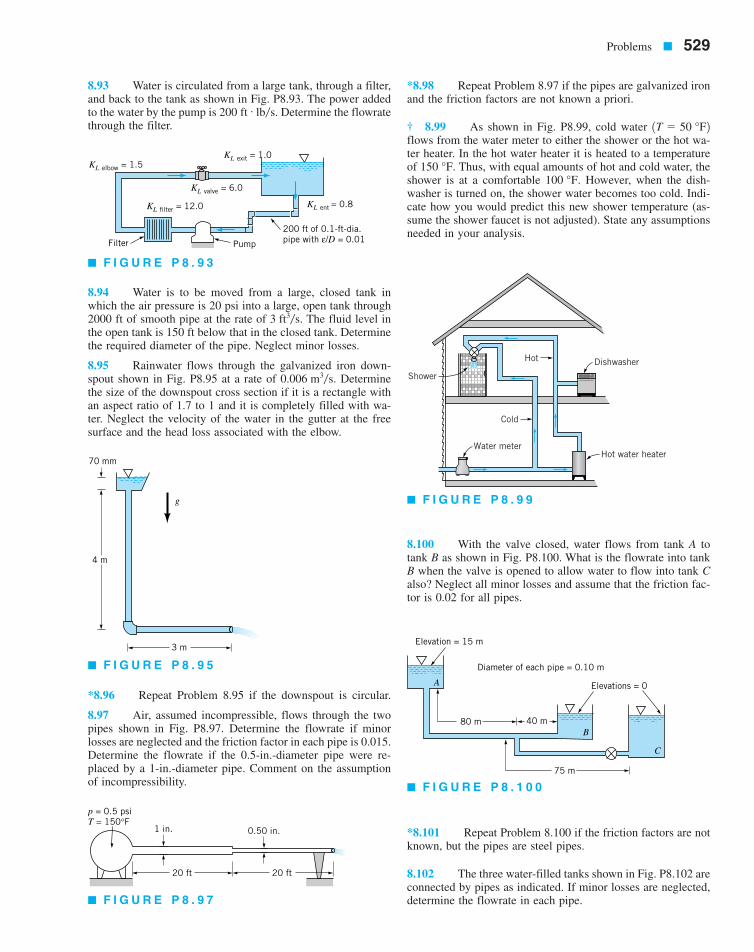
Problems � 529
Water meter
Shower
Hot water heater
DishwasherHot
Cold
� F I G U R E P 8 . 9 9
PumpFilter
KL elbow = 1.5KL exit = 1.0
KL ent = 0.8
KL valve = 6.0
KL filter = 12.0
200 ft of 0.1-ft-dia.pipe with ε/D = 0.01
� F I G U R E P 8 . 9 3
80 m 40 m
75 m
C
B
A Elevations = 0
Elevation = 15 m
Diameter of each pipe = 0.10 m
� F I G U R E P 8 . 1 0 0
p = 0.5 psiT = 150°F
20 ft 20 ft
1 in. 0.50 in.
� F I G U R E P 8 . 9 7
g
70 mm
4 m
3 m
� F I G U R E P 8 . 9 5
*8.96 Repeat Problem 8.95 if the downspout is circular.
8.97 Air, assumed incompressible, flows through the twopipes shown in Fig. P8.97. Determine the flowrate if minorlosses are neglected and the friction factor in each pipe is 0.015.Determine the flowrate if the 0.5-in.-diameter pipe were re-placed by a 1-in.-diameter pipe. Comment on the assumptionof incompressibility.
8.93 Water is circulated from a large tank, through a filter,and back to the tank as shown in Fig. P8.93. The power addedto the water by the pump is Determine the flowratethrough the filter.
200 ft # lb�s.
8.94 Water is to be moved from a large, closed tank inwhich the air pressure is 20 psi into a large, open tank through2000 ft of smooth pipe at the rate of The fluid level inthe open tank is 150 ft below that in the closed tank. Determinethe required diameter of the pipe. Neglect minor losses.
8.95 Rainwater flows through the galvanized iron down-spout shown in Fig. P8.95 at a rate of Determinethe size of the downspout cross section if it is a rectangle withan aspect ratio of 1.7 to 1 and it is completely filled with wa-ter. Neglect the velocity of the water in the gutter at the freesurface and the head loss associated with the elbow.
0.006 m3�s.
3 ft3�s.
*8.98 Repeat Problem 8.97 if the pipes are galvanized ironand the friction factors are not known a priori.
† 8.99 As shown in Fig. P8.99, cold water flows from the water meter to either the shower or the hot wa-ter heater. In the hot water heater it is heated to a temperatureof Thus, with equal amounts of hot and cold water, theshower is at a comfortable However, when the dish-washer is turned on, the shower water becomes too cold. Indi-cate how you would predict this new shower temperature (as-sume the shower faucet is not adjusted). State any assumptionsneeded in your analysis.
100 °F.150 °F.
1T � 50 °F2
8.100 With the valve closed, water flows from tank A totank B as shown in Fig. P8.100. What is the flowrate into tankB when the valve is opened to allow water to flow into tank Calso? Neglect all minor losses and assume that the friction fac-tor is 0.02 for all pipes.
*8.101 Repeat Problem 8.100 if the friction factors are notknown, but the pipes are steel pipes.
8.102 The three water-filled tanks shown in Fig. P8.102 areconnected by pipes as indicated. If minor losses are neglected,determine the flowrate in each pipe.
7708d_c08_529 8/17/01 3:06 PM Page 529
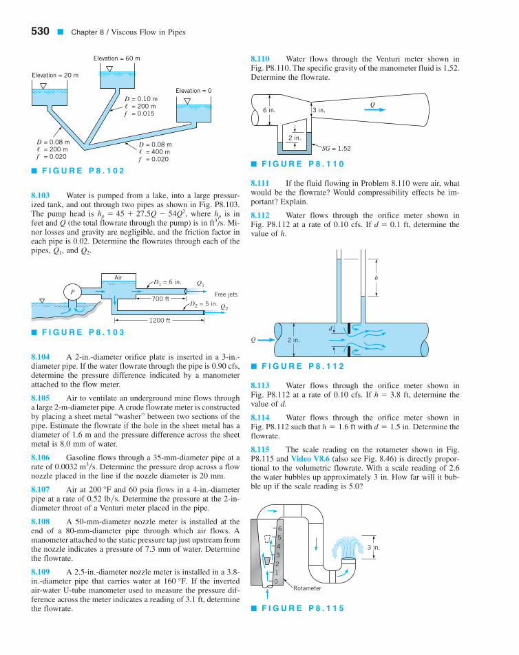
8.103 Water is pumped from a lake, into a large pressur-ized tank, and out through two pipes as shown in Fig. P8.103.The pump head is where is infeet and Q (the total flowrate through the pump) is in Mi-nor losses and gravity are negligible, and the friction factor ineach pipe is 0.02. Determine the flowrates through each of thepipes, and Q2.Q1,
ft3/s.hphp � 45 � 27.5Q � 54Q2,
530 � Chapter 8 / Viscous Flow in Pipes
8.110 Water flows through the Venturi meter shown inFig. P8.110. The specific gravity of the manometer fluid is 1.52.Determine the flowrate.Elevation = 20 m
Elevation = 60 m
Elevation = 0= 0.10 m= 200 m= 0.015
D�f
= 0.08 m= 400 m= 0.020
D�f
= 0.08 m= 200 m= 0.020
D�f
� F I G U R E P 8 . 1 0 2
D1 = 6 in.Air
700 ft
Q1
Q2D2 = 5 in.
Free jets
1200 ft
P
� F I G U R E P 8 . 1 0 3
3 in.6 in.
2 in.
SG = 1.52
Q
� F I G U R E P 8 . 1 1 0
h
Q
d
2 in.
� F I G U R E P 8 . 1 1 2
Rotameter
3 in.
0
654321
� F I G U R E P 8 . 1 1 5
8.104 A 2-in.-diameter orifice plate is inserted in a 3-in.-diameter pipe. If the water flowrate through the pipe is 0.90 cfs,determine the pressure difference indicated by a manometerattached to the flow meter.
8.105 Air to ventilate an underground mine flows througha large 2-m-diameter pipe. A crude flowrate meter is constructedby placing a sheet metal “washer” between two sections of thepipe. Estimate the flowrate if the hole in the sheet metal has adiameter of 1.6 m and the pressure difference across the sheetmetal is 8.0 mm of water.
8.106 Gasoline flows through a 35-mm-diameter pipe at arate of Determine the pressure drop across a flownozzle placed in the line if the nozzle diameter is 20 mm.
8.107 Air at and 60 psia flows in a 4-in.-diameterpipe at a rate of 0.52 lb�s. Determine the pressure at the 2-in-diameter throat of a Venturi meter placed in the pipe.
8.108 A 50-mm-diameter nozzle meter is installed at theend of a 80-mm-diameter pipe through which air flows. Amanometer attached to the static pressure tap just upstream fromthe nozzle indicates a pressure of 7.3 mm of water. Determinethe flowrate.
8.109 A 2.5-in.-diameter nozzle meter is installed in a 3.8-in.-diameter pipe that carries water at If the invertedair-water U-tube manometer used to measure the pressure dif-ference across the meter indicates a reading of 3.1 ft, determinethe flowrate.
160 °F.
200 °F
0.0032 m3�s.
8.111 If the fluid flowing in Problem 8.110 were air, whatwould be the flowrate? Would compressibility effects be im-portant? Explain.
8.112 Water flows through the orifice meter shown inFig. P8.112 at a rate of 0.10 cfs. If ft, determine thevalue of h.
d � 0.1
8.113 Water flows through the orifice meter shown inFig. P8.112 at a rate of 0.10 cfs. If ft, determine thevalue of d.
8.114 Water flows through the orifice meter shown inFig. P8.112 such that ft with in. Determine theflowrate.
8.115 The scale reading on the rotameter shown in Fig.P8.115 and Video V8.6 (also see Fig. 8.46) is directly propor-tional to the volumetric flowrate. With a scale reading of 2.6the water bubbles up approximately 3 in. How far will it bub-ble up if the scale reading is 5.0?
d � 1.5h � 1.6
h � 3.8
7708d_c08_530 8/16/01 5:16 PM Page 530

8.116 This problem involves the determination of the fric-tion factor in a pipe for laminar and transitional flow condi-tions. To proceed with this problem, click here in the E-book.
8.117 This problem involves the calibration of an orificemeter and a Venturi meter. To proceed with this problem, clickhere in the E-book.
8.118 This problem involves the flow of water from a tankand through a pipe system. To proceed with this problem, clickhere in the E-book.
Problems � 531
8.119 This problem involves the flow of water pumpedfrom a tank and through a pipe system. To proceed with thisproblem, click here in the E-book.
8.120 This problem involves the pressure distribution in theentrance region of a pipe. To proceed with this problem, clickhere in the E-book.
8.121 This problem involves the power loss due to frictionin a coiled pipe. To proceed with this problem, click here inthe E-book.
7708d_c08_442-531 7/23/01 2:41 PM Page 531