Turnpike Control and Deep Learning

Turnpike Control and Deep Learning

Borjan Geshkovski & Enrique Zuazua

FAU - AvH / CCM - Deusto, Bilbao / [email protected]

[email protected]

paginaspersonales.deusto.es/enrique.zuazua

Second Symposium on Machine Learning and Dynamical SystemsAugust 2020

Fields Institute, Toronto

Zuazua, Geshkovski (FAU - AvH) Turnpike Control and Deep Learning August 2020 1 / 45

Turnpike Control

Outline

1 Turnpike ControlMotivationOrigins and Foundations of Turnpike theoryThe PDE-Turnpike ParadoxLinear PDE revisitedGeneral theoryNonlinear theoryPerspectives and Bibliography

2 Deep learningContinuous-time deep learningAsymptotics without trackingAsymptotics with tracking = Turnpike controlExtensions


Turnpike Control Motivation

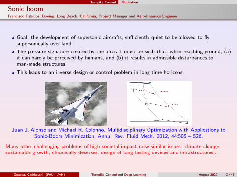
Sonic boomFrancisco Palacios, Boeing, Long Beach, California, Project Manager and Aerodynamics Engineer

Goal: the development of supersonic aircrafts, sufficiently quiet to be allowed to flysupersonically over land.

The pressure signature created by the aircraft must be such that, when reaching ground, (a)it can barely be perceived by humans, and (b) it results in admissible disturbances toman-made structures.

This leads to an inverse design or control problem in long time horizons.

Juan J. Alonso and Michael R. Colonno, Multidisciplinary Optimization with Applications toSonic-Boom Minimization, Annu. Rev. Fluid Mech. 2012, 44:505 – 526.

Many other challenging problems of high societal impact raise similar issues: climate change,sustainable growth, chronically deseases, design of long lasting devices and infrastructures...


Turnpike Control Motivation

Deep learning

Residual neural networks (ResNets) (He et al. ’15) have become the building blocks ofmodern deep learning;

Recent work (E ’17, Haber & Ruthotto ’17, Chen et al. ’18) has reinterpreted ResNets ascontinuous-time controlled nonlinear dynamical systems:

x(t) = f (x(t), u(t)) t ∈ (0,T )

where T > 0 plays the role of the number of layers in the discrete-time setting, f has veryspecific form (sigmoid);

Controls u = u(t), corresponding to the free parameters of the ResNet, found by minimizingan appropriate nonnegative cost function JT (training);

−4 −2 0 2 4xi,1(t)

−4

−2

0

2

xi,

2(t

)

−4 −2 0 2 4xi,1(t)

−4

−2

0

2

xi,

2(t

)

−4 −2 0 2xi,1(t)

−3

−2

−1

0

1

xi,

2(t

)What happens when T →∞, i.e. in the deep, high number of layers regime?1

1Suggested by our FAU colleague Daniel Tenbrinck.


Turnpike Control Origins and Foundations of Turnpike theory

Origins

Although the idea goes back to John von Neumann in 1945, Lionel W. McKenzie traces the termto Robert Dorfman, Paul Samuelson, and Robert Solow’s ”Linear Programming and EconomicsAnalysis” in 1958, referring to an American English word for a Highway:

... There is a fastest route between any two points; and if the origin and destinationare close together and far from the turnpike, the best route may not touch the turnpike.But if the origin and destination are far enough apart, it will always pay to get on to theturnpike and cover distance at the best rate of travel, even if this means adding a littlemileage at either end.


Turnpike Control Origins and Foundations of Turnpike theory

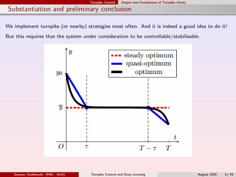
Substantiation and preliminary conclusion

We implement turnpike (or nearby) strategies most often. And it is indeed a good idea to do it!

But this requires that the system under consideration to be controllable/stabilisable.


Turnpike Control The PDE-Turnpike Paradox

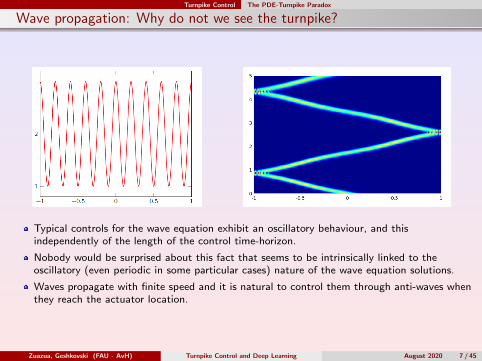
Wave propagation: Why do not we see the turnpike?

Typical controls for the wave equation exhibit an oscillatory behaviour, and thisindependently of the length of the control time-horizon.

Nobody would be surprised about this fact that seems to be intrinsically linked to theoscillatory (even periodic in some particular cases) nature of the wave equation solutions.

Waves propagate with finite speed and it is natural to control them through anti-waves whenthey reach the actuator location.



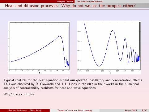
Heat and diffusion processes: Why do not we see the turnpike either?Some PDE examples of lack of turnpike

The heat equation

0 0.1 0.2 0.3 0.4 0.5 0.6 0.7 0.8 0.9 10

0.2

0.4

0.6

0.8

1

t

0.92 0.93 0.94 0.95 0.96 0.97 0.98 0.99 10.05

0.1

0.15

0.2

0.25

t

Typical controls for the heat equation exhibit unexpected oscillatory andconcentration e↵ects. This was observed by R. Glowinski and J. L. Lionsin the 80’s in their works in the numerical analysis of controllabilityproblems for heat and wave equations.Why?

E. Zuazua (FAU - AvH) PDE Control & Time Horizons April 1, 2020 14 / 59

0.92 0.93 0.94 0.95 0.96 0.97 0.98 0.99 10.05

0.1

0.15

0.2

0.25

t

Typical controls for the heat equation exhibit unexpected oscillatory and concentration effects.This was observed by R. Glowinski and J. L. Lions in the 80’s in their works in the numericalanalysis of controllability problems for heat and wave equations.

Why? Lazy controls?



Optimal controls are normally characterised as boundary traces of solutions of the adjointproblem through the optimality system or the Pontryagin Maximum Principle, and solutions ofthe adjoint system of the heat equation

−pt −∆p = 0

look precisely this way.

Large and oscillatory near t = T they decay and get smoother when t gets down to t = 0. Andthis is independent of the time control horizon [0,T ]. The same occurs to wave-like equations

where controls are given by the solutions of the adjoint system

ptt −∆p = 0

that exhibit endless oscillations.

First conclusion:Typical control problems for wave and heat equations do not seem to exhibit the turnpikeproperty.Note however that these are the controls of L2-minimal norm. There are many other possibilitiesfor successful control strategies.


Turnpike Control Linear PDE revisited

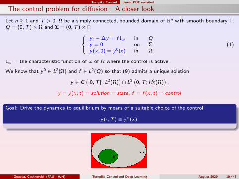
The control problem for diffusion : A closer look

Let n ≥ 1 and T > 0, Ω be a simply connected, bounded domain of Rn with smooth boundary Γ,Q = (0,T )× Ω and Σ = (0,T )× Γ: yt −∆y = f 1ω in Q

y = 0 on Σy(x , 0) = y0(x) in Ω.

(1)

1ω = the characteristic function of ω of Ω where the control is active.

We know that y0 ∈ L2(Ω) and f ∈ L2(Q) so that (9) admits a unique solution

y ∈ C([0,T ] ; L2(Ω)

)∩ L2

(0,T ;H1

0 (Ω)).

y = y(x , t) = solution = state, f = f (x , t) = control

Goal: Drive the dynamics to equilibrium by means of a suitable choice of the control

y(·,T ) ≡ y∗(x).



We address this problem fro a classical optimal control / least square approach:

min1

2

[∫ T

0

∫ω|f |2dxdt +

∫Ω|y(x ,T )− y∗(x)|2dx

].

According to Pontryagin’s Maximum Principle the Optimality System (OS) reads

yt −∆y = ϕ1ω in Q

−ϕt −∆ϕ = 0 in Q

y = 0 on Σ

y(x , 0) = y0(x) in Ω

ϕ(x ,T ) = y(x ,T )− y∗(x) in Ω

ϕ = 0 on Σ.

And the optimal control is:f (x , t) = ϕ(x , t) inω × (0,T ).



The minimizer ϕT saturates the regularity properties required to assure the well-posedness of thefunctional:

H = ϕT : ϕ(x , 0) ∈ L2(Ω)

This is a huge space, allowing an exponential increase of Fourier coefficients at high frequencies.And, because of this, we observe the tendency of the control to concentrate all the action in thefinal time instant t = T , incompatible with turnpike effects2

0 0.1 0.2 0.3 0.4 0.5 0.6 0.7 0.8 0.9 1!3

!2

!1

0

1

2

3

4x 1010

x

Tychonoff’s monster (1935)

2A. Munch & E. Z., Inverse Problems, 2010



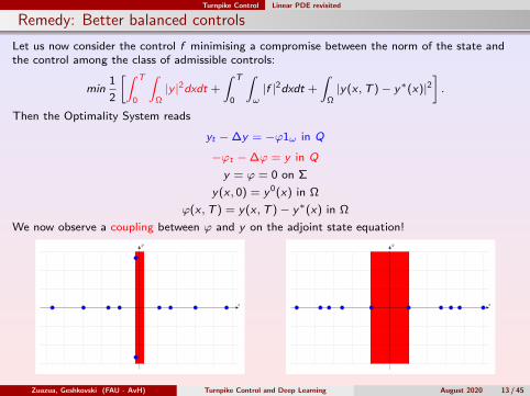
Remedy: Better balanced controls

Let us now consider the control f minimising a compromise between the norm of the state andthe control among the class of admissible controls:

min1

2

[∫ T

0

∫Ω|y |2dxdt +

∫ T

0

∫ω|f |2dxdt +

∫Ω|y(x ,T )− y∗(x)|2

].

Then the Optimality System reads

yt −∆y = −ϕ1ω in Q

−ϕt −∆ϕ = y in Q

y = ϕ = 0 on Σ

y(x , 0) = y0(x) in Ω

ϕ(x ,T ) = y(x ,T )− y∗(x) in Ω

We now observe a coupling between ϕ and y on the adjoint state equation!

x

y

x

y



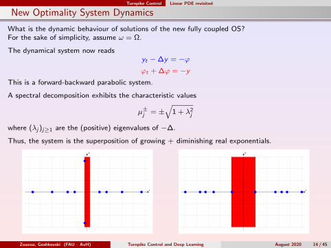
New Optimality System Dynamics

What is the dynamic behaviour of solutions of the new fully coupled OS?For the sake of simplicity, assume ω = Ω.

The dynamical system now readsyt −∆y = −ϕϕt + ∆ϕ = −y

This is a forward-backward parabolic system.

A spectral decomposition exhibits the characteristic values

µ±j = ±√

1 + λ2j

where (λj )j≥1 are the (positive) eigenvalues of −∆.

Thus, the system is the superposition of growing + diminishing real exponentials.

x

y

x

y



The turnpike property for the heat equation

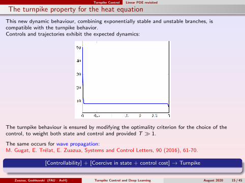
This new dynamic behaviour, combining exponentially stable and unstable branches, iscompatible with the turnpike behavior.Controls and trajectories exhibit the expected dynamics:

The turnpike behaviour is ensured by modifying the optimality criterion for the choice of thecontrol, to weight both state and control and provided T 1.

The same occurs for wave propagation:M. Gugat, E. Trelat, E. Zuazua, Systems and Control Letters, 90 (2016), 61-70.

[Controllability] + [Coercive in state + control cost] → Turnpike



Mainly motivated by applications to economic models and game theory there was a literatureconcerned with this kind of stationary behavior in the transient time for long horizon controlproblems. In that context, such type of result goes under the name of turnpike theory which wasmostly investigated in the finite dimensional case.

A. J. Zaslavski, Turnpike properties in the calculus of variations and optimal control. NonconvexOptimization and its Applications, 80. Springer, New York, 2006.

L. Grune, Economic receding horizon control without terminal constraints Automatica, 49,725-734, 2013

But our main motivation originated from the optimal shape design in aeronautics and other PDEproblems.

In recent years a number of model cases have been well understood in the infinite dimensionalPDE context. But there is still a long way to go...

Dakar 2019


Turnpike Control General theory

Linear theory. Joint work with A. Porretta, SIAM J. Cont. Optim., 2013.

The same methods apply in the inifinite-dimensional context, covering in particular linear heatand wave equations

Consider the finite dimensional dynamicsxt + Ax = Bu

x(0) = x0 ∈ RN(2)

where A ∈ M(N,N), B ∈ M(N,M), with control u ∈ L2(0,T ;RM).Given a matrix C ∈ M(N,N), and some x∗ ∈ RN , consider the optimal control problem

minu

JT (u) =1

2

∫ T

0(|u(t)|2 + |C(x(t)− x∗)|2)dt .

There exists a unique optimal control u(t) in L2(0,T ;RM), characterized by the optimalitycondition

u = −B∗p ,xt + Ax = −BB∗px(0) = x0

,

−pt + A∗p = C∗C(x − x∗)

p(T ) = 0(3)



The steady state control problem

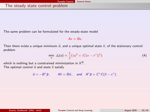
The same problem can be formulated for the steady-state model

Ax = Bu.

Then there exists a unique minimum u, and a unique optimal state x , of the stationary controlproblem

minu

Js(u) =1

2(|u|2 + |C(x − x∗)|2) (4)

which is nothing but a constrained minimization in RN .The optimal control u and state x satisfy

u = −B∗p , Ax = Bu , and A∗p = C∗C(x − x∗) .



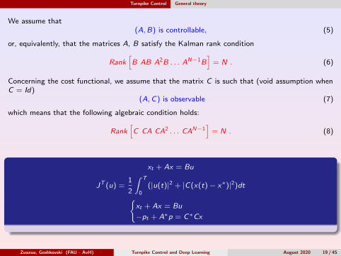
We assume that(A,B) is controllable, (5)

or, equivalently, that the matrices A, B satisfy the Kalman rank condition

Rank[B AB A2B . . . AN−1B

]= N . (6)

Concerning the cost functional, we assume that the matrix C is such that (void assumption whenC = Id)

(A,C) is observable (7)

which means that the following algebraic condition holds:

Rank[C CA CA2 . . . CAN−1

]= N . (8)

xt + Ax = Bu

JT (u) =1

2

∫ T

0(|u(t)|2 + |C(x(t)− x∗)|2)dt

xt + Ax = Bu

−pt + A∗p = C∗Cx



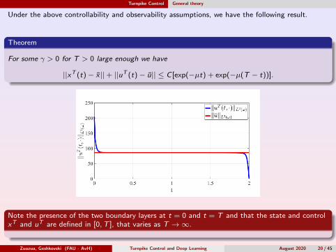
Under the above controllability and observability assumptions, we have the following result.

Theorem

For some γ > 0 for T > 0 large enough we have

||xT (t)− x ||+ ||uT (t)− u|| ≤ C [exp(−µt) + exp(−µ(T − t))].

Note the presence of the two boundary layers at t = 0 and t = T and that the state and controlxT and uT are defined in [0,T ], that varies as T →∞.



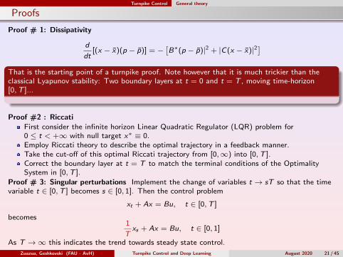
Proofs

Proof # 1: Dissipativity

d

dt[(x − x)(p − p)] = −

[B∗(p − p)|2 + |C(x − x)|2

]That is the starting point of a turnpike proof. Note however that it is much trickier than theclassical Lyapunov stability: Two boundary layers at t = 0 and t = T , moving time-horizon[0,T ]...

Proof #2 : RiccatiFirst consider the infinite horizon Linear Quadratic Regulator (LQR) problem for0 ≤ t < +∞ with null target x∗ ≡ 0.Employ Riccati theory to describe the optimal trajectory in a feedback manner.Take the cut-off of this optimal Riccati trajectory from [0,∞) into [0,T ].Correct the boundary layer at t = T to match the terminal conditions of the OptimalitySystem in [0,T ].

Proof # 3: Singular perturbations Implement the change of variables t → sT so that the timevariable t ∈ [0,T ] becomes s ∈ [0, 1]. Then the control problem

xt + Ax = Bu, t ∈ [0,T ]

becomes1

Txs + Ax = Bu, t ∈ [0, 1]

As T →∞ this indicates the trend towards steady state control.



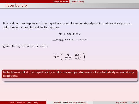
Hyperbolicity

It is a direct consequence of the hyperbolicity of the underlying dynamics, whose steady statesolutions are characterised by the system

Ax + BB∗p = 0

−A∗p + C∗Cx = C∗Cx∗

generated by the operator matrix

A =

(A BB∗

C∗C −A∗)

Note however that the hyperbolicity of this matrix operator needs of controllability/observabilityconditions.


Turnpike Control Nonlinear theory

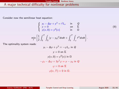
A major technical difficulty for nonlinear problems

Consider now the semilinear heat equation: yt −∆y + y3 = f 1ω in Qy = 0 on Σy(x , 0) = y0(x) in Ω

(9)

minf

[1

2

∫ T

0

∫Ω|y − yd |2dxdt +

∫ T

0

∫ωf 2dxdt

].

The optimality system reads:yt −∆y + y3 = −ϕ1ω in Q

y = 0 on Σ

y(x , 0) = y0(x) in Ω

−ϕt −∆ϕ+ 3y2ϕ = y − yd in Q

ϕ = 0 on Σ

ϕ(x ,T ) = 0 in Ω.


Turnpike Control Nonlinear theory

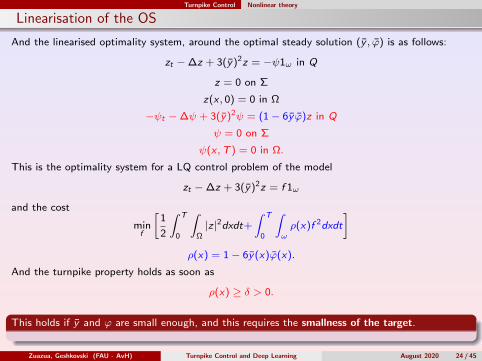
Linearisation of the OS

And the linearised optimality system, around the optimal steady solution (y , ϕ) is as follows:

zt −∆z + 3(y)2z = −ψ1ω in Q

z = 0 on Σ

z(x , 0) = 0 in Ω

−ψt −∆ψ + 3(y)2ψ = (1− 6y ϕ)z in Q

ψ = 0 on Σ

ψ(x ,T ) = 0 in Ω.

This is the optimality system for a LQ control problem of the model

zt −∆z + 3(y)2z = f 1ω

and the cost

minf

[1

2

∫ T

0

∫Ω|z|2dxdt+

∫ T

0

∫ωρ(x)f 2dxdt

]ρ(x) = 1− 6y(x)ϕ(x).

And the turnpike property holds as soon as

ρ(x) ≥ δ > 0.

This holds if y and ϕ are small enough, and this requires the smallness of the target.


Turnpike Control Perspectives and Bibliography

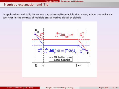
Heuristic explanation and Tip

In applications and daily life we use a quasi-turnpike principle that is very robust and universaltoo, even in the context of multiple steady optima (local or global).



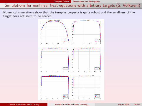
Simulations for nonlinear heat equations with arbitrary targets (S. Volkwein)

Numerical simulations show that the turnpike property is quite robust and the smallness of thetarget does not seem to be needed.



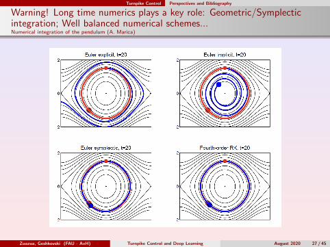
Warning! Long time numerics plays a key role: Geometric/Symplecticintegration; Well balanced numerical schemes...Numerical integration of the pendulum (A. Marica)



An open problem and biblio

Further extend the turnpike theory for nonlinear PDE, getting rid of the smallness condition onthe target, which in numerical simulations seems to be unnecessary.

A. Porretta, E. Z., SIAM J. Control. Optim., 51 (6) (2013), 4242-4273.A. Porretta, E. Z., Springer INdAM Series ”Mathematical Paradigms of Climate Science”, F.Ancona et al. eds, 15, 2016, 67-89.E. Trelat, E. Z., JDE, 218 (2015) , 81-114.M. Gugat, E. Trelat, E. Z., Systems and Control Letters, 90 (2016), 61-70.E. Z., Annual Reviews in Control, 44 (2017) 199-210.E.Trelat, C. Zhang, E. Z., SIAM J. Control Optim. 56 (2018), no. 2, 1222–1252.V. Hernandez-Santamaria, M. Lazar, E.Z. Numerische Mathematik (2019) 141:455-493.D. Pighin, N. Sakamoto, E. Z., IEEE CDC Proceedings, Nice, 2019.G. Lance, E. Trelat, E. Z., Systems & Control Letters 142 (2020) 104733.J. Heiland, E. Z., arXiv:2007.13621, 2020.C. Esteve, H. Kouhkouh, D. Pighin, E. Z., arxiv.org/pdf/2006.10430, 2020.M. Gugat, M. Schuster and E. Z., SEMA/SIMAI Springer Series, 2020.

And further interesting work by collaborators: S. Zamorano (NS), M. Warma & S. Zamorano,Fractional heat,...

Our thanks to our FAU colleague Daniel Tenbrinck. He suggested to us to explore turnpike forNeural Networks.


Deep learning

Outline

1 Turnpike ControlMotivationOrigins and Foundations of Turnpike theoryThe PDE-Turnpike ParadoxLinear PDE revisitedGeneral theoryNonlinear theoryPerspectives and Bibliography

2 Deep learningContinuous-time deep learningAsymptotics without trackingAsymptotics with tracking = Turnpike controlExtensions


Deep learning Continuous-time deep learning

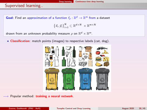
Supervised learning..

Goal: Find an approximation of a function fρ : Rd → Rm from a dataset~xi , ~yi

Ni=1⊂ Rd×N × Rm×N

drawn from an unknown probability measure ρ on Rd × Rm.

Classification: match points (images) to respective labels (cat, dog).

−→ Popular method: training a neural network.



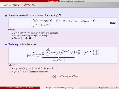
..via neural networks

1 A neural network is a scheme: for any i ≤ Nxk+1i = σ(wkxki + bk ) for k ∈ 0, . . . ,Nlayers − 1

x0i = ~xi ∈ Rd ,

(NN)

wherewk ∈ Rdk+1×dk and bk ∈ Rdk are controlsσ(x) = tanh(x) or σ(x) = maxx, 0Nlayers ≥ 1 depth

2 Training: minimize cost:

infwk ,bkNlayers

k=0

1

N

N∑i=1

loss(ϕ(

xNlayers

i

), ~yi

)︸︷︷︸

:=φ(

xNlayers

)+α

2

∥∥∥wk , bkk

∥∥∥2

`2

wheree.g. loss(x, y) = ‖x − y‖p

`pfor p = 1, 2;

ϕ : Rd → Rm (possibly nonlinear)

ϕ(x) = wNlayers x + bNlayers .



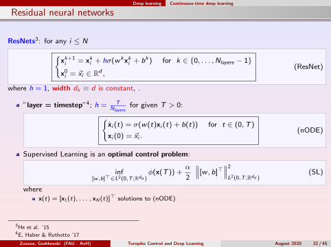
Residual neural networks

ResNets3: for any i ≤ Nxk+1i = xki + hσ(wkxki + bk ) for k ∈ 0, . . . ,Nlayers − 1

x0i = ~xi ∈ Rd ,

(ResNet)

where h = 1, width dk ≡ d is constant, .

”layer = timestep”4; h = TNlayers

for given T > 0:xi (t) = σ(w(t)xi (t) + b(t)) for t ∈ (0,T )

xi (0) = ~xi .(nODE)

Supervised Learning is an optimal control problem:

inf[w,b]>∈L2(0,T ;Rdu )

φ(x(T )) +α

2

∥∥∥[w , b]>∥∥∥2

L2(0,T ;Rdu )(SL)

wherex(t) = [x1(t), . . . , xN (t)]> solutions to (nODE)

3He et al. ’154E, Haber & Ruthotto ’17



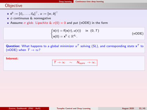
Objective

x0 := [~x1, . . . , ~xN ]>, u := [w , b]>

φ continuous & nonnegative

Asssume σ glob. Lipschitz & σ(0) = 0 and put (nODE) in the formx(t) = f(x(t), u(t)) in (0,T )

x(0) = x0 ∈ Rdx .(nODE)

Question: What happens to a global minimizer uT solving (SL), and corresponding state xT to(nODE) when T →∞?

Interest:T →∞ ∼ Nlayers →∞.



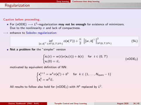
Regularization

Caution before proceeding..

For (nODE) −→ L2–regularization may not be enough for existence of minimizers.Due to the nonlinearity σ and lack of compactness.

−→ enhance to Sobolev regularization:

inf[w,b]>∈H1(0,T ;Rdu )

φ(x(T )) +α

2

∥∥∥[w , b]>∥∥∥2

H1(0,T ;Rdu )(SL)

Not a problem for the ”simpler” versionxi (t) = w(t)σ(xi (t)) + b(t) for t ∈ (0,T )

xi (0) = ~xi ,(nODE2)

motivated by equivalent definition of NN:xk+1i = wkσ(xki ) + bk for k ∈ 1, . . . ,Nlayers − 1

x0i = w0~xi .

All results to follow also hold for (nODE2) with H1 replaced by L2.


Deep learning Asymptotics without tracking

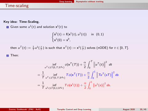
Time-scaling

Key idea: Time-Scaling.

1 Given some u1(t) and solution x1(t) tox1(t) = f(x1(t), u1(t)) in (0, 1)

x1(0) = x0,

then uT (t) := 1Tu1( t

T) is such that xT (t) := x1( t

T) solves (nODE) for t ∈ [0,T ].

2 Then:

infuT∈L2(0,T ;Rdu )

φ(xT (T )) +α

2

∫ T

0

∥∥∥uT (t)∥∥∥2

dt

=1

Tinf

uT∈L2(0,T ;Rdu )Tφ(xT (T )) +

α

2

∫ 1

0

∥∥∥TuT (sT )∥∥∥2

ds

=1

Tinf

u1∈L2(0,1;Rdu )Tφ(x1(1)) +

α

2

∫ 1

0

∥∥u1(s)∥∥2

ds.



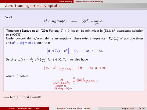
Zero training error asymptotics

Recall:x† ∈ arg min(φ) ⇐⇒ φ(x†) = min

Rdxφ.

Theorem (Esteve et al. ’20): For any T > 0, let uT be minimizer in (SL), xT associated solutionto (nODE).Under controllability/reachability assumptions, there exist a sequence Tn+∞

n=1 of positive times

and x† ∈ arg min(φ), such that∥∥∥xTn (Tn)− x†∥∥∥ −→ 0 as n→∞.

Setting un(t) = 1Tn

uTn ( tTn

) for t ∈ [0,Tn], we also have∥∥un − u1∥∥H1(0,1;Rdu )

−→ 0 as n→∞

where u1 solvesinf

u∈H1(0,1;Rdu )subject to

x(1) ∈arg min(φ)

α

2‖u‖2

H1(0,1;Rdu ).

−→ Not a turnpike result!



Figure: Here Nlayers =⌊T

32

⌋and thus h = 1√

T, and we consider α = 1.


Deep learning Asymptotics with tracking = Turnpike control

Turnpike

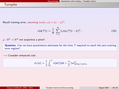
Recall training error, assuming loss(x , y) = ‖x − y‖2:

φ(x(T )) :=1

N

N∑i=1

‖ϕ(xi (T ))− ~yi‖2 ; (10)

ϕ : Rd → Rm not surjective a priori!

Question: Can we have quantitative estimates for the time T required to reach the zero trainingerror regime?

−→ Consider enhanced cost

JT (u) :=1

2

∫ T

0φ(x(t))dt +

α

2‖u‖2

H1(0,T ;Rdu )



The optimal steady states

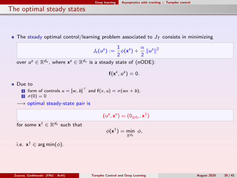
The steady optimal control/learning problem associated to JT consists in minimizing

Js(us) :=1

2φ(xs) +

α

2‖us‖2

over us ∈ Rdu , where xs ∈ Rdx is a steady state of (nODE):

f(xs , us) = 0.

Due to1 form of controls u = [w , b]> and f(x, u) = σ(wx + b);2 σ(0) = 0

−→ optimal steady-state pair is

(us , xs) = (0Rdu , x†)

for some x† ∈ Rdx such thatφ(x†) = min

Rdxφ,

i.e. x† ∈ arg min(φ).



Turnpike property

Theorem (Esteve et al. ’20): Under controllability/reachability assumptions, for anysufficiently large T > 0, consider a solution uT to

infu∈H1(0,T ;Rdu )

1

2

∫ T

0φ(x(t))dt +

α

2‖u‖2

H1(0,T ;Rdu )

and let xT be the associated state, solution to (nODE).Then ∥∥∥uT∥∥∥

H1(0,T ;Rdu )≤ C

and there exists x† ∈ arg min(φ) such that∥∥∥xT (t)− x†∥∥∥ ≤ γ (e−µt + e−µ(T−t)

)∀t ∈ [0,T ] and for some C > 0, γ > 0 and µ > 0, all independent of T .

Due to the absence of final time cost:

Corollary (Esteve et al. ’20): In fact,∥∥∥xT (t)− xd

∥∥∥ ≤ γ e−µt∀t ∈ [0,T ] and for some γ > 0 and µ > 0 independent of T .



−3 −2 −1 0 1xi,1(t)

−2

−1

0

1

xi,

2(t

)

T =20.0

−3 −2 −1 0 1xi,1(t)

−2

−1

0

1

xi,

2(t

)

T =20.0

−1 0 1 2 3xi,1(t)

−1.5

−1.0

−0.5

0.0

0.5

1.0

xi,

2(t

)

T =20.0

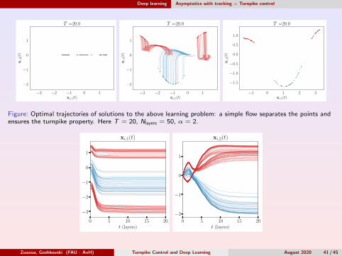
Figure: Optimal trajectories of solutions to the above learning problem: a simple flow separates the points andensures the turnpike property. Here T = 20, Nlayers = 50, α = 2.

0 5 10 15 20t (layers)

−3

−2

−1

0

1

xi,1(t)

0 5 10 15 20t (layers)

−2

−1

0

1

xi,2(t)


Deep learning Extensions

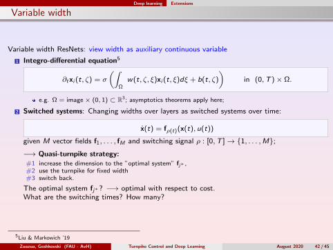
Variable width

Variable width ResNets: view width as auxiliary continuous variable

1 Integro-differential equation5

∂txi (t, ζ) = σ

(∫Ω

w(t, ζ, ξ)xi (t, ξ)dξ + b(t, ζ)

)in (0,T )× Ω.

e.g. Ω = image× (0, 1) ⊂ R3; asymptotics theorems apply here;

2 Switched systems: Changing widths over layers as switched systems over time:

x(t) = fρ(t)(x(t), u(t))

given M vector fields f1, . . . , fM and switching signal ρ : [0,T ]→ 1, . . . ,M;

−→ Quasi-turnpike strategy:#1 increase the dimension to the ”optimal system” fj∗ ,#2 use the turnpike for fixed width#3 switch back.

The optimal system fj∗? −→ optimal with respect to cost.What are the switching times? How many?

5Liu & Markowich ’19


Deep learning Extensions

Outlook

1 Long-time behavior depends on the cost functional to be minimized.

2 Results should be complemented by ML subfields (e.g. CNN design, training algorithms..)

Many other open problems and extensive bibliography can be found in our paper:

https://arxiv.org/abs/2008.02491


https://arxiv.org/abs/2008.02491

Team, collaborators, funding

E. Trelat (Paris Sorbonne), A. Porretta (Roma 2), M. Gugat (FAU), D. Pighin (Innovalia),C. Esteve (UAM & Deusto), M. Lazar (Dubrovnik), V. Hernandez-Santamaria, N. Sakamoto(Nanzan), J. Heiland (Magdeburg), H. Kouhkouh (Padova), M. Schuster (FAU).

Funded by the ERC Advanced Grant DyCon and an Alexander von Humboldt Professorshipand Marie-Sklodowska Curie ITN ”ConFlex”


Thank you for your attention.


Documents

Turnpike Control and Deep Learning