MODEL BASED LEARNING OF SIGMA POINTS IN UNSCENTED KALMAN FILTERING

 Ryan Turner and Carl Edward Rasmussen

University of Cambridge

Department of Engineering

Trumpington Street, Cambridge CB2 1PZ, UK

ABSTRACT

The unscented Kalman filter (UKF) is a widely used method

in control and time series applications. The UKF suffers

from arbitrary parameters necessary for a step known as

sigma point placement, causing it to perform poorly in non-

linear problems. We show how to treat sigma point place-

ment in a UKF as a learning problem in a model based view.

We demonstrate that learning to place the sigma points cor-

rectly from data can make sigma point collapse much less

likely. Learning can result in a significant increase in pre-

dictive performance over default settings of the parameters

in the UKF and other filters designed to avoid the problems

of the UKF, such as the GP-ADF. At the same time, we

maintain a lower computational complexity than the other

methods. We call our method UKF-L.

1. INTRODUCTION

Filtering in linear dynamical systems (LDS) and nonlinear

dynamical systems (NLDS) is frequently used in many ar-

eas, such as signal processing, state estimation, control, and

finance/econometric models. Filtering (inference) aims to

estimate the state of a system from a stream of noisy mea-

surements. Imagine tracking the location of a car based on

odometer and GPS sensors, both of which are noisy. Se-

quential measurements from both sensors are combined to

overcome the noise in the system and to obtain an accurate

estimate of the system state. Even when the full state is

only partially measured, it can still be inferred; in the car

example the engine temperature is unobserved, but can be

inferred via the nonlinear relationship from acceleration. To

exploit this relationship appropriately, inference techniques

in nonlinear models are required; they play an important

role in many practical applications.

LDS and NLDS belong to a class of models known as

state-space models. A state-space model assumes that there

exists a sequence of latent states xt that evolve over time

according to a Markovian process specified by a transition

function f . The latent states are observed indirectly in ytthrough a measurement function g. We consider state-space

models given by

xt = f (xt−1) + , xt ∈ RM ,

yt = g(xt) + ν  , yt ∈ RD .(1)

Here, the system noise ∼ N (0,Σ) and the measurement

noise ν  ∼ N (0,Σν ) are both Gaussian. In the LDS case,

f  and g are linear functions, whereas the NLDS covers the

general nonlinear case.

Kalman filtering [1] corresponds to exact (and fast) in-

ference in the LDS, however it can only model a limited set

of phenomena. For the last few decades, there has been in-

terest in NLDS for more general applicability. In the state-

space formulation, the nonlinear systems do not generally

yield analytically tractable algorithms.

The most widely used approximations for filtering in

NLDS are the extended Kalman filter (EKF) [2] and the un-

scented Kalman filter (UKF) [3]. The EKF linearizes f  and

g at the current estimate of  xt and treats the system as a

nonstationary linear system even though it is not. The UKF

propagates several estimates of  xt through f  and g and re-

constructs a Gaussian distribution assuming the propagated

values came from a linear system. The locations of the esti-

mates of xt are known as the sigma points. Many heuristics

have been developed to help set the sigma point locations

[4]. Unlike the EKF, the UKF has free parameters that de-

termine where to put the sigma points. The key idea in this

paper, is that the UKF and EKF are doing exact inference in

a model that is somewhat perverted from the original model

described in the state-space formulation. The interpretation

of EKF and UKF as models, not just approximate methods,

allows us to better identify their underlying assumptions. It

also enables us to learn the free parameters in the UKF in

a model based manner from training data. If the settings

of the sigma point are a poor fit to the underlying dynam-

ical system, the UKF can make horrendously poor predic-

tions. This paper’s contribution is a strategy for improving

the UKF through a novel learning algorithm for appropriate

sigma point placement: we call this method UKF-L.

 

2. UNSCENTED KALMAN FILTERING

We first review how filtering and the UKF works and then

explain the UKF’s generative assumptions. Filtering meth-

ods consist of three steps: time update, prediction step, and

measurement update. They iterate in a predictor-corrector

setup. In the time update we find p(xt|y1:t−1):

 p(xt|y1:t−1) =

 

p(xt|xt−1) p(xt−1|y1:t−1) dxt−1 , (2)

using p(xt−1|y1:t−1). In the prediction step we predict the

observed space, p(yt|y1:t−1) using p(xt|y1:t−1):

 p(yt|y1:t−1) =

 

p(yt|xt) p(xt|y1:t−1) dxt . (3)

Finally, in the measurement update we find p(xt|yt) using

information from how good (or bad) the prediction in the

prediction step is:

 p(xt|y1:t) ∝  p(yt|xt) p(xt|y1:t−1) . (4)

In the linear case all of these equations can be done ana-

lytically using matrix multiplications. The EKF explicitly

linearizes f  and g at the point E [xt] at each step. The

UKF uses the whole distribution on xt, not just the mean,

to place sigma points and implicitly linearize the dynamics,

which we call the unscented transform (UT). In one dimen-

sion the sigma points roughly correspond to the mean and

α-standard deviation points; the UKF generalizes this idea

to higher dimensions. The exact placement of sigma points

depends on the unitless parameters {α ,β ,κ} ∈ R+ through

X 0 := µ, X i := µ ± ( 

(D + λ)Σ)i (5)

λ := α2(D + κ)−D , (6)

where√ ·i refers to the ith row of the Cholesky factoriza-

tion.1 The sigma points have weights assigned by:

w0m := λ/(D + λ), w0

c := λ/(D + λ) + (1 − α2 + β )

wim := wi

c := 1/2(D + λ) , (7)

where wm is used to reconstruct the predicted mean and wc

used for the predicted covariance. We can loosely interpret

the unscented transform as approximating the input distri-

bution by 2D + 1 point masses at X with weight w. Once

the sigma points X , have been calculated the filter accesses

f  and g as black boxes to find Y t, either f (X t) or g(X t)depending on the step. The UKF reconstructs the mean and

variance of the propagated distribution from Y t had  the dy-

namics been linear. It does not guarantee the moments will

match the moment of the true non-Gaussian distribution.

1If √ P  = A ⇒ P  = AA, then we use the rows in (5). If P  =

AA, then we use the columns.

Algorithm 1 Sampling data from UKF’s implicit model

1: p(x1|∅) ← (µ0,Σ0)2: for t = 1 to T  do

3: Prediction step: p(yt|y1:t−1) using p(xt|y1:t−1)4: Sample yt from prediction step distribution

5: Measurement update: p(xt|y1:t) using yt6: Time update: find p(xt+1|y1:t) using p(xt|y1:t)7: end for

Both the EKF and the UKF approximate the nonlinear

state-space as a nonstationary linear system. The UKF de-

fines its own generative process that linearizes the nonlinear

function f and g wherever in xt a UKF filtering the time se-

ries would expect xt to be. Therefore, it is possible to sam-

ple synthetic data from the UKF by sampling from its one-

step-ahead predictions as seen in Algorithm 1. The sam-

pling procedure augments the filter: predict-sample-correct.

If we use the UKF with the same {α ,β ,κ} used to generate

synthetic data, then the one-step-ahead predictive distribu-

tion will be the exact same distribution the data point was

sampled from.

2.1. Setting the parameters

We summarize all the parameters as θ := {α ,β ,κ}. For any

setting of  θ the UKF will give identical predictions to the

Kalman filter if f  and g are both linear. Many of the heuris-

tics for setting θ assume f  and g are linear (or close to it),

which is not the problem the UKF solves. For example, one

of the heuristics for setting θ is that β = 2 is optimal if the

state distribution p(xt|y1:t) is exactly Gaussian [5]. How-

ever, the state distribution will seldom be Gaussian unless

the system is linear, in which case any setting of θ is exact!

It is often recommended to set the parameters to α = 1,

β = 0, and κ = 2.

3. THE ACHILLES’ HEEL OF THE UKF

The UKF can have very poor performance because its pre-

dictive variances can be far too small if the sigma points

are placed in inconvenient locations. A too small predictive

variance will cause observations to have too much weight

in the measurement update, which causes the UKF to fit to

noise. Meaning, the UKF will perform poorly even when

evaluated on root-mean-square-error (RMSE), which only

uses the predictive mean.

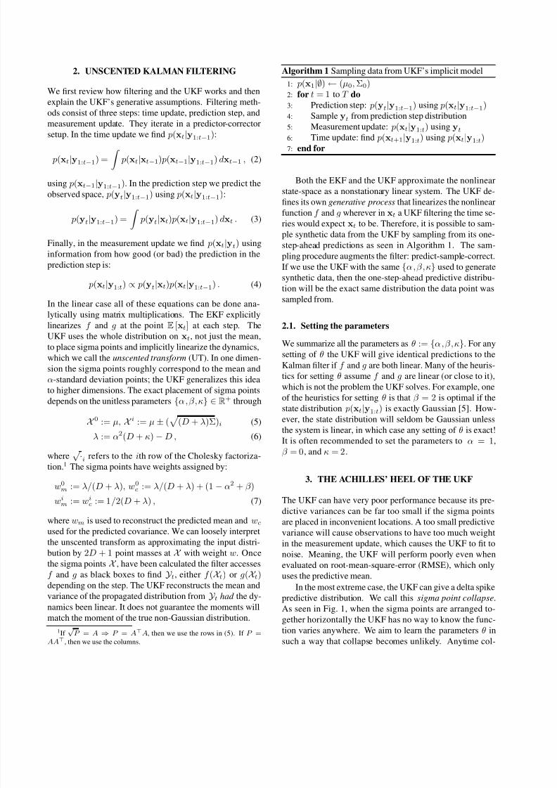
In the most extreme case, the UKF can give a delta spike

predictive distribution. We call this sigma point collapse.

As seen in Fig. 1, when the sigma points are arranged to-

gether horizontally the UKF has no way to know the func-

tion varies anywhere. We aim to learn the parameters θ in

such a way that collapse becomes unlikely. Anytime col-

 

lapse happens in training the marginal likelihood will be

very low. Hence, the learned parameters will avoid any-

where this delta spike occurred in training. Maximizing the

marginal likelihood is tricky since it is not well behaved for

settings of θ that cause sigma point collapse.

−1

−0.5

0

0.5

1

−10 −5 0 5 10

−10 −5 0 5 10

Fig. 1. An illustration of a good and bad assignment of 

sigma points. The lower panel shows the true input distri-

bution. The center panel shows the sinusoidal system func-

tion f  (blue) and the sigma points for α = 1 (red crosses)

and α = 0.68 (green rings). The left panel shows the true

output distribution (shaded), the output distribution under

α = 1 (red spike) and α = 0.68 (green). Using a different

set of sigma points we can get either a completely degener-

ate solution (a delta spike) or a near optimal approximation

within the class of Gaussian approximations.

4. MODEL BASED LEARNING

A common approach to estimating model parameters θ in

general is to maximize the log marginal likelihood

(θ) := log p(y1:T |θ) =T 

t=1

log p(yt|y1:t−1, θ) . (8)

Hence we can equivalently maximize the sum from the one-

step-ahead predictions. One might be tempted to apply a

gradient based optimizer on (8), but as seen in Fig. 2 the

marginal likelihood can be very noisy. The noise, or in-

stability in the likelihood, is likely the result of the phe-

nomenon explained in Section 3, where a slight change in

parameterization can avoid problematic sigma point place-

ment. This makes the application of a gradient-based opti-

mizer hopeless.

It is also possible to apply Markov chain Monte Carlo

(MCMC) and integrate out the parameters. However, this

is usually overkill as the posterior on θ is usually highly

peaked unless T  is very small. Tempering must be used as

mixing will be difficult if the chain is not initialized inside

the posterior peak. Even in the case when T  is small enough

to spread the posterior out, we would still like a single point

estimate for computational speed on the test set. 2

We will focus on learning using a Gaussian process (GP)

based optimizer [6]. Since the marginal likelihood surface

has an underlying smooth function but contains what amounts

to additive noise, a probabilistic regression method seems a

natural fit for finding the maximum.

5. GAUSSIAN PROCESS OPTIMIZERS

Gaussian processes form a prior over functions. Estimat-

ing the parameters amounts to finding the maximum of a

structured function: the log marginal likelihood. Therefore,

it seems natural to use a prior over functions to guide our

search. The same principle has been applied to integration

in [7].

GP optimization (GPO) allows for effective derivative

 free optimization. We consider the maximization of a like-

lihood function (θ). GPs allow for derivative information

∂ θ to be included as well, but in our case that will not be

very useful due to the function’s instability.

GPO treats optimization as a sequential decision prob-

lem in a probabilistic setting, receiving reward r when us-

ing the right input θ to get a large function value output

(θ). At each step GPO uses its posterior over the objective

function p((θ)) to look for θ it believes have large function

value (θ). A maximization strategy that is greedy will al-

ways evaluate the function  p((θ)) where the mean function

E [(θ)] is the largest. A strategy that trades-off  exploration

with exploitation will take into account the posterior vari-

ance Var [(θ)]. Areas of θ with high variance carry a possi-

bility of having a large function value or high reward r. The

optimizer is programmed to evaluate at the maxima of 

J (θ) := E [(θ)] + K  

Var [(θ)] , (9)

where K is a constant to control the exploration exploitation

trade-off. The optimizer must also find the maximum of  J ,but since it is a combination of the GP mean and variance

functions it is easy to optimize with gradient methods.

6. EXPERIMENTS AND RESULTS

We test our method on filtering in three dynamical systems:

the sinusoidal dynamics used in [8], the Kitagawa dynamics

used in [9, 10], and pendulum dynamics used in [9]. The

sinusoidal dynamics are described by

xt+1 = 3 sin(xt) + w, w ∼ N (0, 0.12) , (10)

yt = σ(xt/3) + v, v ∼ N (0, 0.12) . (11)

2If we want to integrate the parameters out we must run the UKF with

each sample of θ|y1:T  during test and average. To get the optimal point

estimate of the posterior we would like to compute the Bayes’ point .

 

0 1 2 3 40

2

4

6

8

   l  o  g   l   i   k  e   l   i   h  o  o   d   (  n  a   t  s   /  o   b  s   )

0 1 2 3 4−2.5

−2

−1.5

−1

−0.5

   D

(a) α ∈ (0.1, 4)

0 1 2 3 40

0.5

1

   l  o  g   l   i   k  e   l   i   h  o  o   d   (  n  a   t  s   /  o   b  s   )

0 1 2 3 4−1.5

−1

−0.5

   D

(b) β ∈ (0, 4)

1 2 3 4 5

0

1

2

   l  o  g   l   i   k  e   l   i   h  o  o   d   (  n  a   t  s   /  o   b  s   )

1 2 3 4 5

−2

−1

0

   D

(c) κ ∈ (0.1, 5)

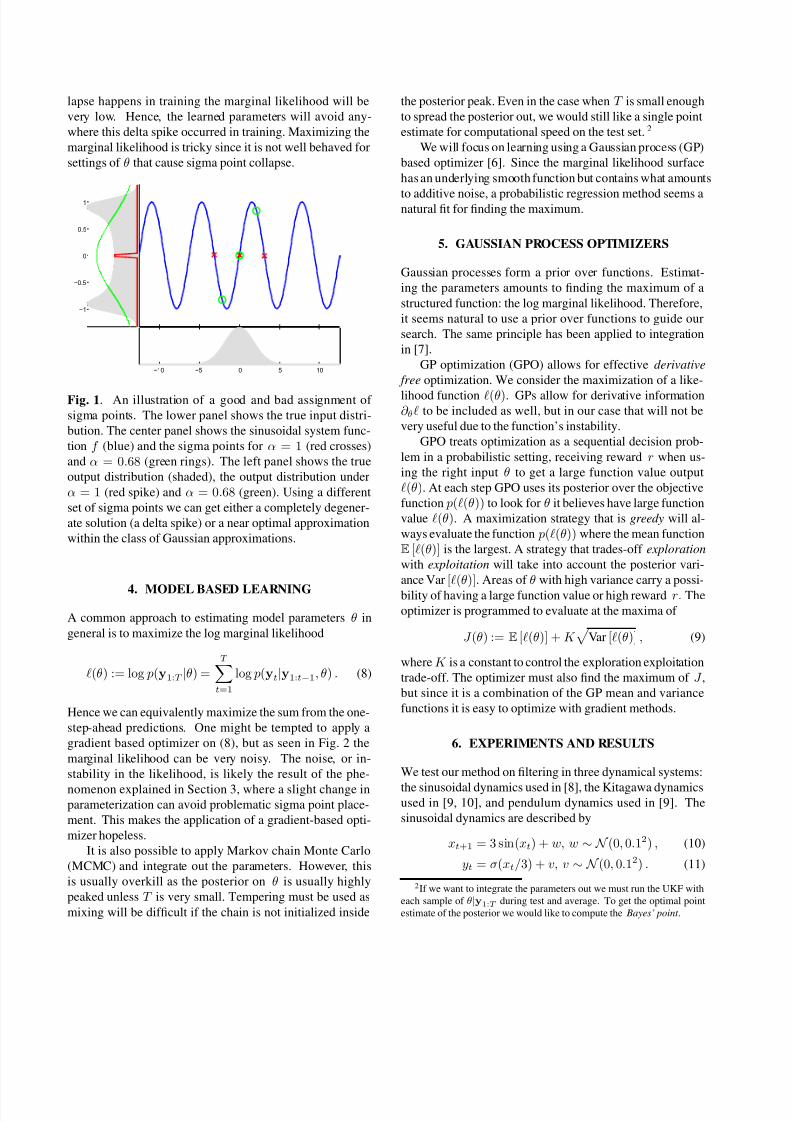
Fig. 2. Illustration of the UKF when applied to a pendulum system. Cross section of the marginal likelihood (blue line)

varying the parameters one at a time from the defaults (red vertical line). We shift the marginal likelihood, in nats/observation,

to make the lowest value zero. The dashed green line is the total variance diagnostic D := E [log(|Σ|/|Σ0|)], where Σ is the

predictive variance in one-step-ahead prediction. We divide out the variance Σ0 of the time series when treating it as iid to

make D unitless. Values of θ with small predictive variances closely track the θ with low marginal likelihood.

where σ(·) represents a sigmoid. The Kitagawa model is

described by

xt+1 = 0.5xt +25xt

1 + x2t

+ w, w ∼ N (0, 0.22) , (12)

yt = 5 sin(2xt) + v, v ∼ N (0, 0.012) . (13)

The Kitagawa model was presented as filtering problem in

[10]. The pendulum dynamics is described by a discretized

ordinary differential equation (ODE) at ∆t = 400ms. The

pendulum possesses a mass m = 1 k g and a length l =1 m. The pendulum angle ϕ is measured anti-clockwise

from hanging down. The state x = [ϕ, ϕ̇] of the pen-

dulum is given by the angle ϕ and the angular velocity ϕ̇.

The ODE is

d

dt

ϕ̇ϕ

=

−mlg sinϕml2

ϕ̇

, (14)

where g the acceleration of gravity. This model is com-

monly used in stochastic control for the inverted pendulum

problem [11]. The measurement function is

yt =

arctan

 p1−l sin(ϕt) p1−l cos(ϕt)

arctan

 p2−l sin(ϕt) p2−l cos(ϕt)

,

 p1 p2

=

1−2

, (15)

which corresponds to bearings only measurement  since we

do not directly observe the velocity. We use system noise

Σw = diag([0.12 0.32]) and Σv = diag([0.22 0.22]) as ob-

servation noise.

For all the problems we compare to UKF-D, EKF, the

GP-UKF, and GP-ADF, and the time independent model

(TIM); we use UKF-D to denote a UKF with default pa-

rameter settings, and UKF-L for learned parameters. The

TIM treats the data as iid normal and is inserted as a refer-

ence point. The GP-UKF and GP-ADF use GPs to approx-

imate f  and g and exploit the properties of GPs to make

tractable predictions. The Kitagawa and pendulum dynam-

ics were used by [9] to illustrate the performance of the GP-

ADF and the very poor performance of the UKF. [9] used

the default settings of  α = 1, β  = 0, κ = 2 for all of 

the experiments. We used exploration trade off  K  = 2 for

the GPO in all the experiments. Additionally, GPO used

the squared-exponential with automatic relevance determi-

nation (SE-ARD) covariance function plus a noise term of 

0.01 nats/observation. We set the GPO to have a maximum

number of function evaluations of 100, even better results

can be obtained by letting the optimizer run longer to hone

the parameter estimate. We show that by learning appro-

priate values for θ we can match, if not exceed, the perfor-

mance of the GP-ADF and other methods.

The models were evaluated on one-step-ahead predic-

tion. The evaluation metrics were the negative log-predictive

likelihood (NLL), the mean squared error (MSE), and the

mean absolute error (MAE) between the mean of the pre-

diction and the true value. Note that unlike the NLL, the

MSE and MAE do not account for uncertainty. The MAE

will be more difficult for approximate methods than MSE.

For MSE, the optimal action is to predict the mean of the

predictive distribution, while for the MAE it is the median.

Most approximate methods attempt to moment match to a

Gaussian and preserve the mean; the median of the true pre-

dictive distribution is implicitly assumed to be the same as

mean. Quantitative results are shown in Table 1.

6.1. Sinusoidal dynamics

The models were trained on T  = 1000 observations from

the sinusoidal dynamics, and tested on R = 10 restarts

with T  = 500 points each. The initial state was sampled

from a standard normal x1 ∼ N (0, 1). The UKF optimizer

found the optimal values α = 2.0216, β  = 0.2434, and

κ = 0.4871.

 

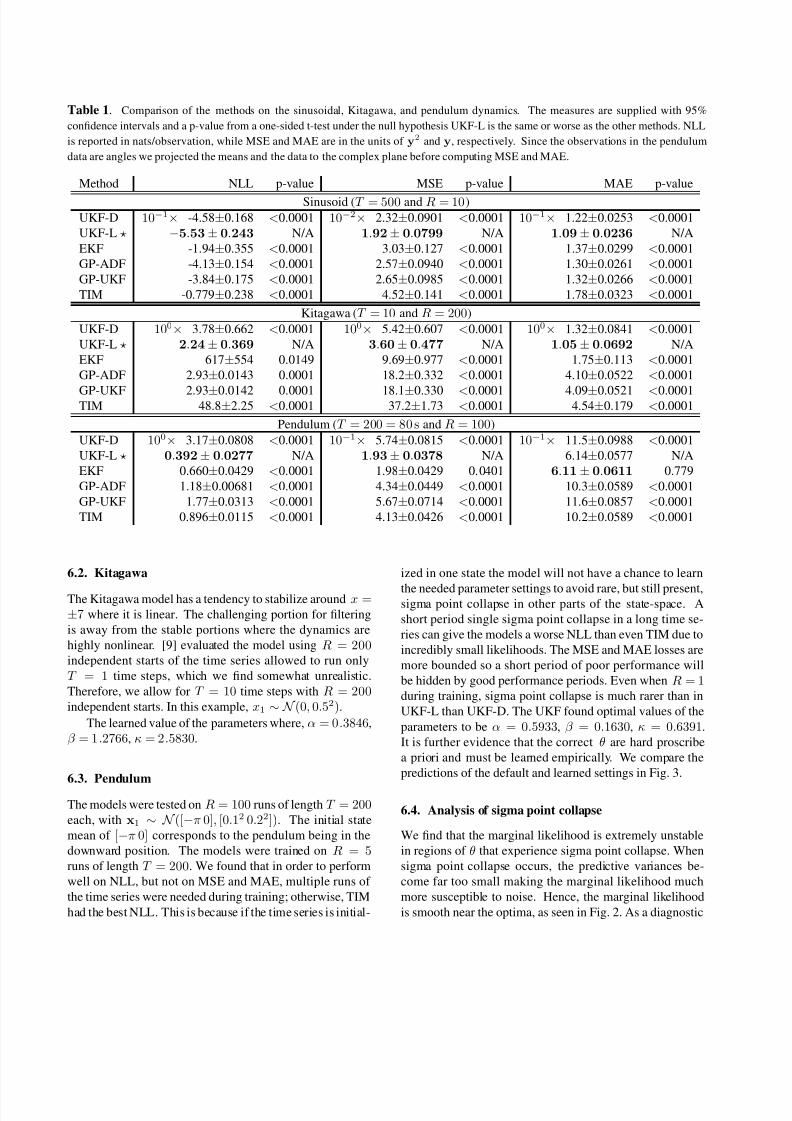
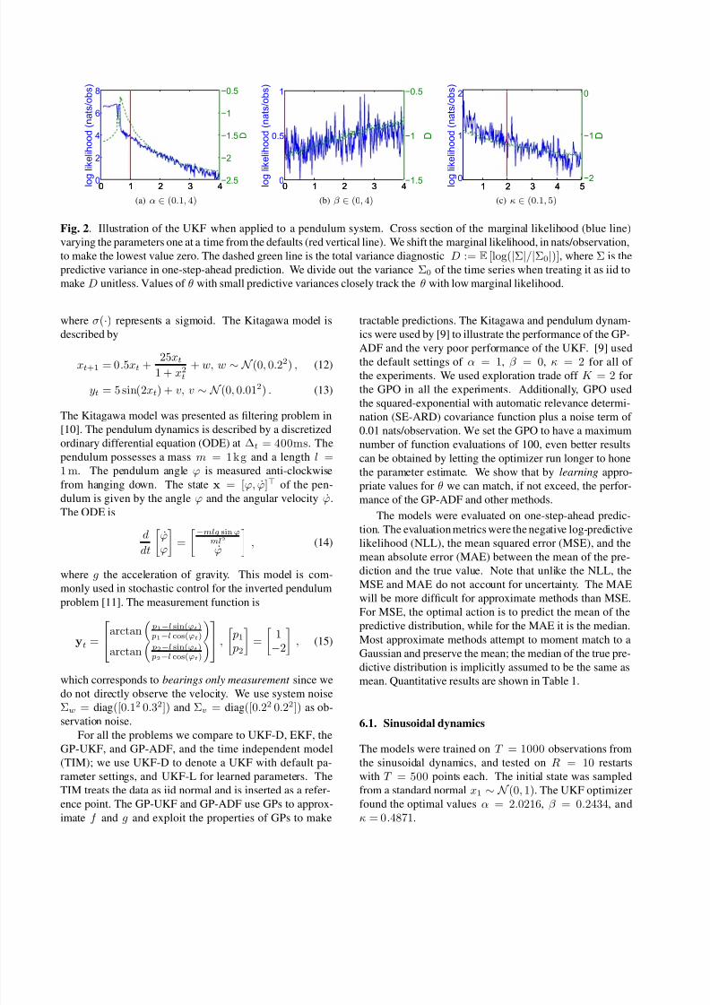
Table 1. Comparison of the methods on the sinusoidal, Kitagawa, and pendulum dynamics. The measures are supplied with 95%

confidence intervals and a p-value from a one-sided t-test under the null hypothesis UKF-L is the same or worse as the other methods. NLL

is reported in nats/observation, while MSE and MAE are in the units of y2 and y, respectively. Since the observations in the pendulum

data are angles we projected the means and the data to the complex plane before computing MSE and MAE.

Method NLL p-value MSE p-value MAE p-value

Sinusoid (T  = 500 and R = 10)

UKF-D 10−1× -4.58±0.168 <0.0001 10−2× 2.32±0.0901 <0.0001 10−1× 1.22±0.0253 <0.0001

UKF-L −5.53± 0.243 N/A 1.92± 0.0799 N/A 1.09± 0.0236 N/A

EKF -1.94±0.355 <0.0001 3.03±0.127 <0.0001 1.37±0.0299 <0.0001

GP-ADF -4.13±0.154 <0.0001 2.57±0.0940 <0.0001 1.30±0.0261 <0.0001

GP-UKF -3.84±0.175 <0.0001 2.65±0.0985 <0.0001 1.32±0.0266 <0.0001

TIM -0.779±0.238 <0.0001 4.52±0.141 <0.0001 1.78±0.0323 <0.0001

Kitagawa (T  = 10 and R = 200)

UKF-D 100× 3.78±0.662 <0.0001 100× 5.42±0.607 <0.0001 100× 1.32±0.0841 <0.0001

UKF-L 2.24± 0.369 N/A 3.60± 0.477 N/A 1.05± 0.0692 N/A

EKF 617±554 0.0149 9.69±0.977 <0.0001 1.75±0.113 <0.0001

GP-ADF 2.93±0.0143 0.0001 18.2±0.332 <0.0001 4.10±0.0522 <0.0001

GP-UKF 2.93±0.0142 0.0001 18.1±0.330 <0.0001 4.09±0.0521 <0.0001

TIM 48.8±2.25 <0.0001 37.2±1.73 <0.0001 4.54±0.179 <0.0001

Pendulum (T  = 200 = 80 s and R = 100)

UKF-D 100× 3.17±0.0808 <0.0001 10−1× 5.74±0.0815 <0.0001 10−1× 11.5±0.0988 <0.0001

UKF-L 0.392± 0.0277 N/A 1.93± 0.0378 N/A 6.14±0.0577 N/A

EKF 0.660±0.0429 <0.0001 1.98±0.0429 0.0401 6.11± 0.0611 0.779

GP-ADF 1.18±0.00681 <0.0001 4.34±0.0449 <0.0001 10.3±0.0589 <0.0001

GP-UKF 1.77±0.0313 <0.0001 5.67±0.0714 <0.0001 11.6±0.0857 <0.0001

TIM 0.896±0.0115 <0.0001 4.13±0.0426 <0.0001 10.2±0.0589 <0.0001

6.2. Kitagawa

The Kitagawa model has a tendency to stabilize around x =±7 where it is linear. The challenging portion for filtering

is away from the stable portions where the dynamics are

highly nonlinear. [9] evaluated the model using R = 200independent starts of the time series allowed to run only

T  = 1 time steps, which we find somewhat unrealistic.

Therefore, we allow for T  = 10 time steps with R = 200independent starts. In this example, x1 ∼ N (0, 0.52).

The learned value of the parameters where, α = 0.3846,

β = 1.2766, κ = 2.5830.

6.3. Pendulum

The models were tested on R = 100 runs of length T  = 200each, with x1 ∼ N ([−π 0], [0.12 0.22]). The initial state

mean of  [−π 0] corresponds to the pendulum being in the

downward position. The models were trained on R = 5runs of length T  = 200. We found that in order to perform

well on NLL, but not on MSE and MAE, multiple runs of 

the time series were needed during training; otherwise, TIM

had the best NLL. This is because if the time series is initial-

ized in one state the model will not have a chance to learn

the needed parameter settings to avoid rare, but still present,

sigma point collapse in other parts of the state-space. A

short period single sigma point collapse in a long time se-

ries can give the models a worse NLL than even TIM due to

incredibly small likelihoods. The MSE and MAE losses are

more bounded so a short period of poor performance will

be hidden by good performance periods. Even when R = 1during training, sigma point collapse is much rarer than in

UKF-L than UKF-D. The UKF found optimal values of the

parameters to be α = 0.5933, β  = 0.1630, κ = 0.6391.

It is further evidence that the correct θ are hard proscribe

a priori and must be learned empirically. We compare the

predictions of the default and learned settings in Fig. 3.

6.4. Analysis of sigma point collapse

We find that the marginal likelihood is extremely unstable

in regions of θ that experience sigma point collapse. When

sigma point collapse occurs, the predictive variances be-

come far too small making the marginal likelihood much

more susceptible to noise. Hence, the marginal likelihood

is smooth near the optima, as seen in Fig. 2. As a diagnostic

 

1 96 1 98 2 00 2 02 2 04 2 06 2 08 2 10 2 12 2 14

−0.5

0

0.5

1

1.5

2

Time step

      x        1

(a) Default θ

1 96 1 98 200 2 02 204 206 20 8 210 2 12

−0.5

0

0.5

1

1.5

2

Time step

      x        1

(b) Learned θ

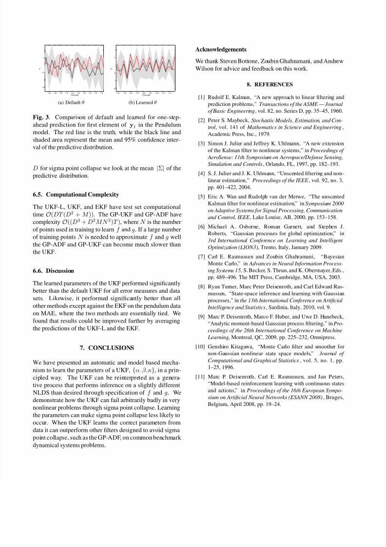
Fig. 3. Comparison of default and learned for one-step-

ahead prediction for first element of  yt in the Pendulum

model. The red line is the truth, while the black line and

shaded area represent the mean and 95% confidence inter-

val of the predictive distribution.

D for sigma point collapse we look at the mean |Σ| of the

predictive distribution.

6.5. Computational Complexity

The UKF-L, UKF, and EKF have test set computational

time O(DT (D2 + M )). The GP-UKF and GP-ADF have

complexity O((D3 + D2MN 2)T ), where N  is the number

of points used in training to learn f  and g. If a large number

of training points N  is needed to approximate f  and g well

the GP-ADF and GP-UKF can become much slower than

the UKF.

6.6. Discussion

The learned parameters of the UKF performed significantly

better than the default UKF for all error measures and data

sets. Likewise, it performed significantly better than all

other methods except against the EKF on the pendulum data

on MAE, where the two methods are essentially tied. We

found that results could be improved further by averaging

the predictions of the UKF-L and the EKF.

7. CONCLUSIONS

We have presented an automatic and model based mecha-

nism to learn the parameters of a UKF, {α.β,κ}, in a prin-

cipled way. The UKF can be reinterpreted as a genera-

tive process that performs inference on a slightly different

NLDS than desired through specification of  f  and g. We

demonstrate how the UKF can fail arbitrarily badly in very

nonlinear problems through sigma point collapse. Learning

the parameters can make sigma point collapse less likely to

occur. When the UKF learns the correct parameters from

data it can outperform other filters designed to avoid sigma

point collapse, such as the GP-ADF, on common benchmark 

dynamical systems problems.

Acknowledgements

We thank Steven Bottone, Zoubin Ghahramani, and Andrew

Wilson for advice and feedback on this work.

8. REFERENCES

[1] Rudolf E. Kalman, “A new approach to linear filtering and

prediction problems,” Transactions of the ASME — Journal

of Basic Engineering, vol. 82, no. Series D, pp. 35–45, 1960.

[2] Peter S. Maybeck, Stochastic Models, Estimation, and Con-

trol, vol. 141 of  Mathematics in Science and Engineering ,

Academic Press, Inc., 1979.

[3] Simon J. Julier and Jeffrey K. Uhlmann, “A new extension

of the Kalman filter to nonlinear systems,” in Proceedings of 

 AeroSense: 11th Symposium on Aerospace/Defense Sensing,

Simulation and Controls , Orlando, FL, 1997, pp. 182–193.

[4] S. J. Julier and J. K. Uhlmann, “Unscented filtering and non-

linear estimation,” Proceedings of the IEEE , vol. 92, no. 3,

pp. 401–422, 2004.

[5] Eric A. Wan and Rudolph van der Merwe, “The unscented

Kalman filter for nonlinear estimation,” in Symposium 2000

on Adaptive Systems for Signal Processing, Communication

and Control, IEEE , Lake Louise, AB, 2000, pp. 153–158.

[6] Michael A. Osborne, Roman Garnett, and Stephen J.

Roberts, “Gaussian processes for global optimization,” in

3rd International Conference on Learning and Intelligent 

Optimization (LION3), Trento, Italy, January 2009.

[7] Carl E. Rasmussen and Zoubin Ghahramani, “Bayesian

Monte Carlo,” in Advances in Neural Information Process-

ing Systems 15, S. Becker, S. Thrun, and K. Obermayer, Eds.,

pp. 489–496. The MIT Press, Cambridge, MA, USA, 2003.

[8] Ryan Turner, Marc Peter Deisenroth, and Carl Edward Ras-

mussen, “State-space inference and learning with Gaussian

processes,” in the 13th International Conference on Artificial

 Intelligence and Statistics, Sardinia, Italy, 2010, vol. 9.

[9] Marc P. Deisenroth, Marco F. Huber, and Uwe D. Hanebeck,

“Analytic moment-based Gaussian process filtering,” in Pro-

ceedings of the 26th International Conference on Machine

 Learning, Montreal, QC, 2009, pp. 225–232, Omnipress.

[10] Genshiro Kitagawa, “Monte Carlo filter and smoother for

non-Gaussian nonlinear state space models,” Journal of 

Computational and Graphical Statistics , vol. 5, no. 1, pp.

1–25, 1996.

[11] Marc P. Deisenroth, Carl E. Rasmussen, and Jan Peters,

“Model-based reinforcement learning with continuous states

and actions,” in Proceedings of the 16th European Sympo-

sium on Artificial Neural Networks (ESANN 2008) , Bruges,

Belgium, April 2008, pp. 19–24.