1

TUTORIAL #1

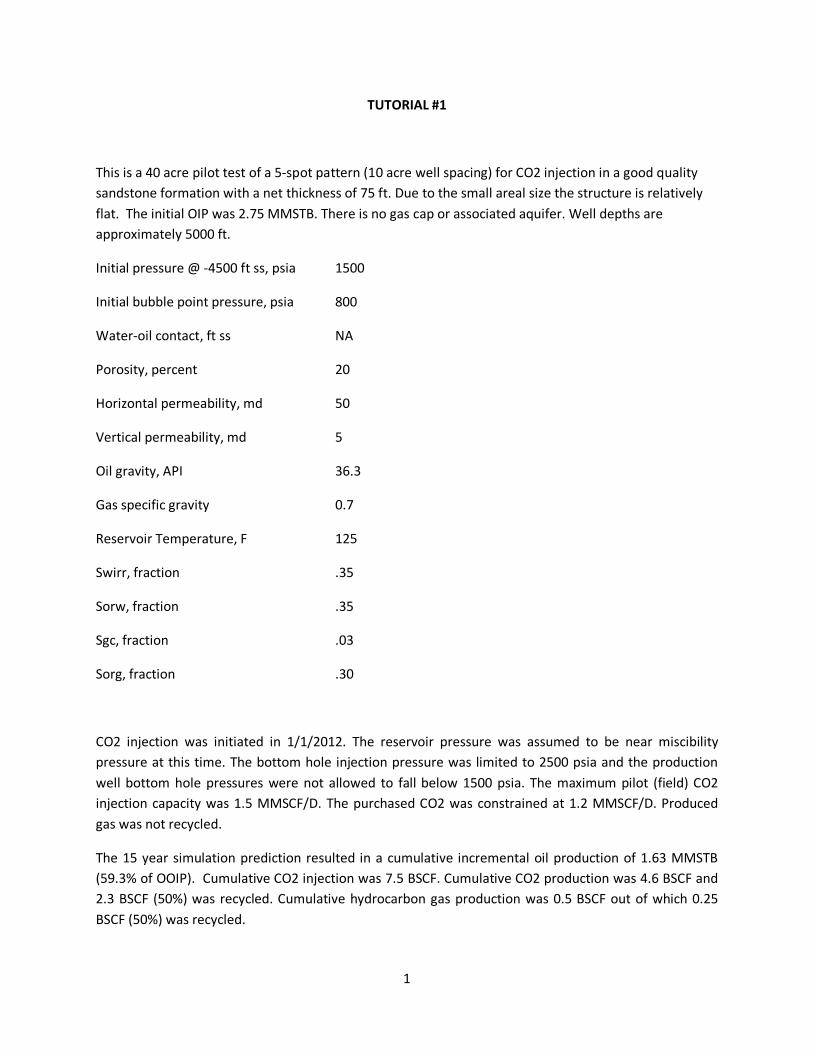
This is a 40 acre pilot test of a 5-spot pattern (10 acre well spacing) for CO2 injection in a good quality

sandstone formation with a net thickness of 75 ft. Due to the small areal size the structure is relatively

flat. The initial OIP was 2.75 MMSTB. There is no gas cap or associated aquifer. Well depths are

approximately 5000 ft.

Initial pressure @ -4500 ft ss, psia 1500

Initial bubble point pressure, psia 800

Water-oil contact, ft ss NA

Porosity, percent 20

Horizontal permeability, md 50

Vertical permeability, md 5

Oil gravity, API 36.3

Gas specific gravity 0.7

Reservoir Temperature, F 125

Swirr, fraction .35

Sorw, fraction .35

Sgc, fraction .03

Sorg, fraction .30

CO2 injection was initiated in 1/1/2012. The reservoir pressure was assumed to be near miscibility

pressure at this time. The bottom hole injection pressure was limited to 2500 psia and the production

well bottom hole pressures were not allowed to fall below 1500 psia. The maximum pilot (field) CO2

injection capacity was 1.5 MMSCF/D. The purchased CO2 was constrained at 1.2 MMSCF/D. Produced

gas was not recycled.

The 15 year simulation prediction resulted in a cumulative incremental oil production of 1.63 MMSTB

(59.3% of OOIP). Cumulative CO2 injection was 7.5 BSCF. Cumulative CO2 production was 4.6 BSCF and

2.3 BSCF (50%) was recycled. Cumulative hydrocarbon gas production was 0.5 BSCF out of which 0.25

BSCF (50%) was recycled.

2

Run time was approximately 5 minute elapse time.

In the course of developing the tutorial examples, some COZView screens may have changed slightly

from the views shown in this document. These changes should not impact the model building and

simulation process.

Model Building Process

The process starts with creation of a New Project. Select New Project and provide a project name on the

Home Page.

3

Under the Process Explorer tab, select Structure in the Static Model area. The Create New Layer

Structure window will appear. Input a top layer name and the net thickness (25 for this example). OK will

save the information.

All menus referenced in this tutorial are in the Process Explorer menu area.

The model building starts with the structural surface of the productive formation. Before beginning the

structural model definition, add any additional layers that are required by right-clicking the layer 1 row

in the upper right of the Static Model Structure screen. Select Add New Layer and input the required

data. Repeat the process as needed. In this tutorial, three layers each of thickness 25 ft. are required.

4

The Static Model Structure area allows the user to first Define Contours by using the resizing bars and

rotation control ball. In this example the contours were not modified from the default view.

Save and Continue is recommended.

This is followed by Define Area Boundary (the green area shown below). The simulation model will be

the area inside the green boundaries. The user selects the boundary points to reflect the reservoir area

on the structure top map.

5

Assign Coordinates allows the user to provide coordinate positions for each of the boundary points

provided. These are typically in feet as shown below.

Save and Continue is recommended.

6

Selection of Scaled Model and Assign Elevation/Use Contours allows the user to establish the structural

contour elevations. The shallowest contour elevation (smallest circle) of -4500 ft ss and the deepest

contour elevation of -4550 ft ss establish the contour interval.

Save and Continue is recommended.

The default Minimum Cell Size displayed at the bottom of the Scaled Model area is 330 ft. Based on the

model area boundary dimensions of 1320 ft by 1320 ft assigned previously, this would result in a 4 x 4

cell areal grid. For this example, which will use an injection well in the center of the area, we would

prefer a 5 by 5 cell areal grid. Change the Minimum Cell Size to 250 ft and select Save and Continue.

7

Assign Wells allows the user to position wells on the structural surface. Once all wells are positioned

their KB and TD may be defined (optional). The KB and TD data are

Well KB TD

1 100 5100

2 100 5200

3 100 5100

4 100 5050

5 100 5200

Save and Continue is recommended.

8

Select Layer Properties 3D View to confirm the structural model and well positions in a 3D view.

Layer Properties should be selected from the Static Model menu area. Values will already be input for

the layers previously defined. The default units for each property are shown. The default values can be

changed if appropriate.

Select Done when finished to save the layer properties.

9

PVT should be selected from the Fluid and Saturation Properties menu area. The initial PVT properties

screen will be blank. The New button should be selected to create a new set of PVT properties (table).

The default values must be overridden by the user to create the PVT data shown below when the

Calculate button is selected.

Select Save to save the data.

10

Saturation Functions should be selected from the Fluid and Saturation Properties menu area. The initial

Saturation Function properties screen will be blank. The New button should be selected to create a new

set of Saturation Function properties (table). The default values must be overridden by the user to

create the Saturation Function data shown below when the Generate button is selected.

Select Save to save the data.

11

Model Initialization should be selected from the Verify Model menu area. This screen will initially be

blank. The user can verify the volumetrics of the model that has been created by inputting appropriate

values in the data fields. Initially the volumetrics of the model can be checked for the original conditions,

if desired. This requires identification of the Fluid PVT and Saturation Function tables previously defined.

The following data should be input for the initialization (current) conditions.

Initialization Date 1/1/2012

Model Type 2 phase

Pressure @Ref 1500

Reference Elevation -4500

Elevation @ WOC -5000 (is below the model)

PSATHCG 800

Selection of Initialize Model will provide the results of the volumetric calculation on the View Model

Volumetrics screen. A brief view of the Simulator Runner window will appear before the volumetrics

are reported. An OIP of approximately 2.75 MMSTB should be reported subject to differences in the

user defined model and this example.

Select Done when finished.

If the user is not satisfied with the volumetric values calculated, changes to the model data created to

this point can be made and saved and new volumetrics calculated.

12

The following steps will define well and field operating conditions for the prediction case to be run.

Select Well Location from the Well Data menu area to verify previously input well locations, KB

elevations and TD. This is generally informational reporting only. If additional wells are required, the

user should return to the Static Model menu area and interactively locate the new well(s). KB and TD

values can be change if required.

Select Done to save.

13

Select Completions from the Well Data area to view and alter the well completions if appropriate.

Initially all wells are assumed to be completed in all layers. The Active check box can be unchecked for

any well layer completion, if desired. No completion changes were made to the default values for this

example.

It is important to keep track of the dates shown in the various well and field control screens. These must

be consistent with the Initialization Date (start date for the prediction simulation run). These dates

should be changed if necessary.

If any changes are made to the well completions select Done to save.

14

Select Well Constraints from the Prediction/Well Parameters menu area. This screen will initially be

blank. The Batch Generate button is a fast way to input values for multiple wells. The user can input the

values noted below for the Liquid Producer wells and separately for the GAS/CO2 Injection wells.

Well Constraints

Injection well (Well_5): Center well in the five spot

Maximum Bottom hole pressure (psia) 2500

Maximum CO2 Injection rate (MSCF/day) 5000

Producers (Well_1 – Well_4)

Minimum BHP (psia) 1500

Maximum Production Liquid rate (STB/day) 400

Select Done to save.

15

Select Well Limits from the Prediction/Well Parameters menu area. This screen will initially be blank.

The Batch Generate button is a fast way to input values for multiple wells.

Well limits

Minimum Oil rate (STB/day) 5

Action to take Close well

Select Done to save.

16

Select Field (Facility) Controls from the Prediction Period/Field Parameters menu area. Select New to

establish the Effective Date (start date for Field Controls) and the Injection Gas Type. Please note that

the default Injection Gas Type is CO2 gas. In this tutorial it is required to select CO2 as Injection Gas

Type.

Select OK to continue.

17

Field Controls

Maximum Field Gas Injection Constraint (MSCF/day) 1500

Field Gas Reinjection Fraction 0.5

Available External Injection gas (MSCF/day) 1200

Select Done to save.

18

Select Limits from the Prediction Period/Field Parameters menu area. Check the Active box and input

appropriate values. It is always wise to have a field limit specified such that the simulation run will stop

when the field limit is reached.

Select Done to save.

It is prudent at this stage to return to the various well and field parameter screen to insure that data,

particularly dates, are set appropriately.

19

Select Run Simulation. The Model Initialization date will be shown in the Start Date box. If this is not

correct, return to the Model Initialization screen and reset the date and save. The user must provide a

value in the End Date box. This must be at least one month after the Start Date.

The End Date for this example is 1/1/2027.

Select Go to initiate the simulation run.

The Simulator Runner window will appear and update the CPU activity for the simulation run. DO NOT

close the Simulator Runner window during the simulation run. It can be minimized. Closing the

Simulator runner window will stop the simulation run.

DO NOT close COZView during the simulation run. It can be minimized. Closing COZView will not stop

the simulation run, but the simulation results will not be loaded at the conclusion of the simulation run.

DO NOT change projects in COZView during a simulation run for this same reason. DO NOT turn the

computer off during the simulation run. All simulation results will be lost.

Two files are created early during the simulation run which may help the user track the progress of the

simulation run. These are stored in the COZView directory along with various project database and

result files. The files are Projectname.COZOUT and Projectname.COZDAT. The .COZDAT file is the input

data “deck” prepared by COZView for COZSim. The .COZOUT file reports well production and injection

activity for timesteps during the simulation run. It is update frequently. Both of these files can be

opened with a Text editor. The .COZDAT file can be reviewed to assure that the data “deck” is setup as

20

the user anticipated. The .COZOUT file can be reviewed as the simulation run progresses. If the results

are not as anticipated the run can be stopped in the Simulator Runner window.

An example of the .COZOUT file at the end of this simulation run is shown below.

DO NOT delete are change these files during the simulation run. If the same project is re-run with

changes to some parameters, these files will be overwritten.

When the Simulation Runner window disappears, the simulation run has completed.

At the completion of the simulation run two small windows will appear which advise the user that the

Map and PLT (plot) results are being loaded into COZView.

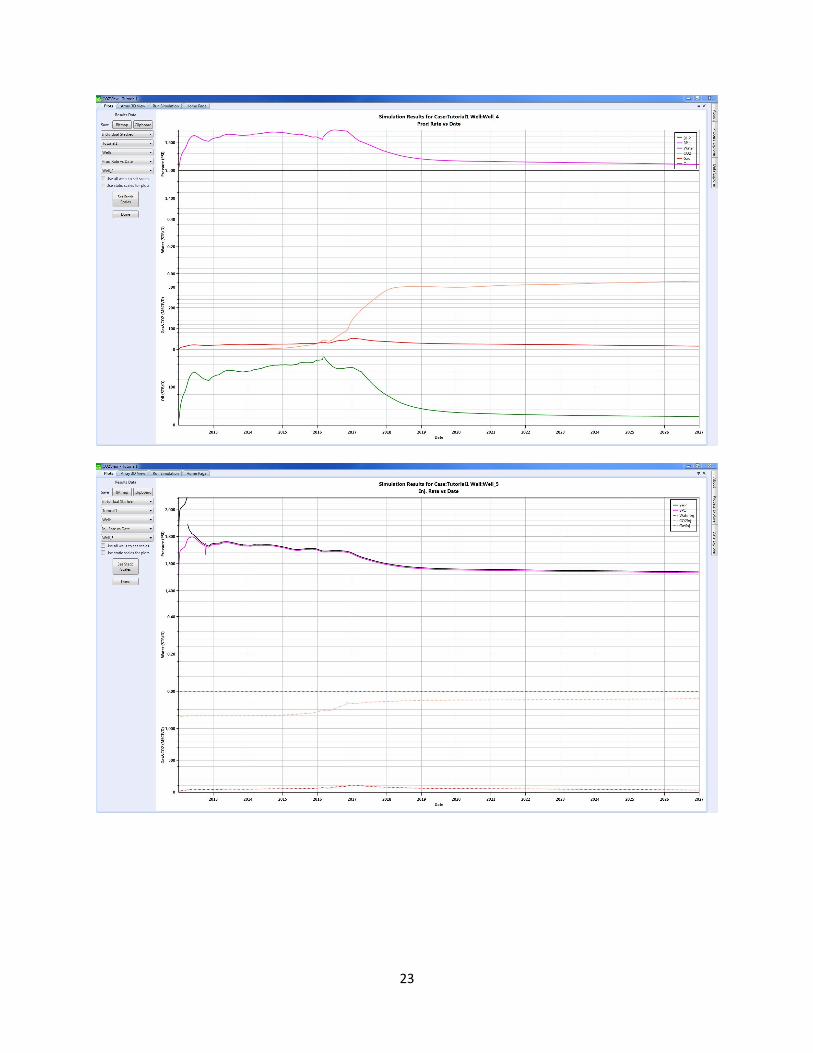
Select Plots from the Simulation Results area. This will give the user access to various simulation plots

for the wells and field. A sample of the available plots for this prediction simulation is shown below.

It has been found prudent to close all menu tabs except the Home Page and save data as may be

requested before selecting any of the Simulation Results menus. This assures that the plot, map and

table files are refreshed and prior results are not shown in error.

21

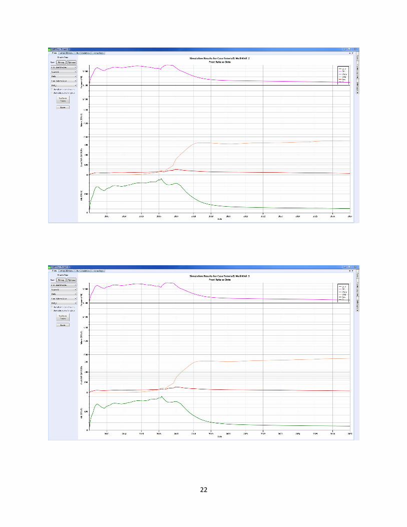
22

23

24

Select Array 3D View from the Simulation Results area. This will give the user access to various

simulation maps for the field. A sample of the available maps for this prediction simulation is shown

below.

25

26

27

The user can also select Tables from the Simulation Results area. This will provide access to tabular

simulation results for wells and the field. These tables can be exported to .csv files for use in

spreadsheet applications.

It is also noted that any plot displays can be saved to Bitmap files or to the Clipboard for pasting into

report documents. Any map displays can be saved to Bitmap files.

Simulation Results

The simulation results for this pilot are very interesting.

First Contact miscibility was achieved (Miscibility index of 1.0) near the injection well as shown in the

Miscibility map in all layers by 1/1/2015. The reservoir pressure map in Layer 1 at 1/1/2015 indicates a

pressure of 1729 psia at the injection well. By 1/1/2027 the Miscibility map in Layer 1 show less than full

miscibility at the injection well. This is due to a decline in the reservoir pressure.

This presents the user with an opportunity to use the model to optimize the pilot performance by better

management of well completions and production practices to maintain miscible conditions in the

reservoir.