Tutorial 2: A simple charged system - ESPResSoespressomd.org/wordpress/wp-content/uploads/2016/10/02-charged... · Tutorial 2: A simple charged system October 9, 2016 Contents 1 Introduction

Tutorial 2: A simple charged system

October 9, 2016

Contents

1 Introduction 2

2 Basic set up 2

3 Equilibration 5

4 Running the simulation 6

5 Analysis 7

6 Task - Real units 9

7 2D Electrostatics and Constraints 10

1

1 Introduction

This tutorial introduces some of the basic features of ESPResSo for charged systems byconstructing a simulation script for a simple salt crystal. In the subsequent task, weuse to a more realistic force-field for a NaCl crystal. Finally, we introduce constraintsand 2D-Electrostatics to simulate a molten salt in a parallel plate capacitor. We assumethat the reader is familiar with the basic concepts of Python and MD simulations. Thecode pieces can be copied step by step into a python script file, which then can be runusing pypresso <file> from the ESPResSo build directory. Note that you might haveto correct erroneous line breaks. Compile espresso with the following features in yourmyconfig.hpp to be set throughout the whole tutorial:

#define EXTERNAL_FORCES

#define CONSTRAINTS

#define MASS

#define ELECTROSTATICS

#define LENNARD_JONES

2 Basic set up

The script for the tutorial can be found in your build directory at\doc\tutorials\python\02-charged_system\nacl.py. We start with setting up allthe relevant simulation parameters in one place:

# System parameters

n_part = 200

n_ionpairs = n_part /2

density = 0.7

time_step = 0.01

temp = 1.0

gamma = 1.0

l_bjerrum = 1.0

num_steps_equilibration = 1000

num_configs = 100

integ_steps_per_config = 1000

# Particle parameters

types = {"Anion": 0, "Cation": 1}

2

numbers = {"Anion": n_ionpairs , "Cation": n_ionpairs}

charges = {"Anion": -1.0, "Cation": 1.0}

lj_sigmas = {"Anion": 1.0, "Cation": 1.0}

lj_epsilons = {"Anion": 1.0, "Cation": 1.0}

WCA_cut = 2.**(1. / 6.)

lj_cuts = {"Anion": WCA_cut * lj_sigmas["Anion"],

"Cation": WCA_cut * lj_sigmas["Cation"]}

These variables do not change anything in the simulation engine, but are just standardPython variables. They are used to increase the readability and flexibility of the script.The box length is not a parameter of this simulation, it is calculated from the numberof particles and the system density. This allows to change the parameters later easily,e. g. to simulate a bigger system. We use dictionaries for all particle related parameters,which is less error-prone and readable as we will see later when we actually need thevalues. The parameters here define a purely repulsive, equally sized, monovalent salt.

The simulation engine itself is modified by changing the espressomd.System() prop-erties. We create an instance system and set the box length, periodicity and time step.The skin depth skin is a parameter for the link–cell system which tunes its performance,but shall not be discussed here. Further, we activate the Langevin thermostat for ourNVT ensemble with temperature temp and friction coefficient gamma.

# Setup System

system = espressomd.System()

box_l = (n_part / density)**(1. / 3.)

system.box_l = [box_l , box_l , box_l]

system.periodicity = [1, 1, 1]

system.time_step = time_step

system.cell_system.skin = 0.3

system.thermostat.set_langevin(kT=temp , gamma=gamma)

We now fill this simulation box with particles at random positions, using type andcharge from our dictionaries. Using the length of the particle list system.part for the id,we make sure that our particles are numbered consecutively. The particle type is usedto link non-bonded interactions to a certain group of particles.

# Place particles

for i in range(n_ionpairs):

system.part.add(

id=len(system.part),

3

type=types["Anion"],

pos=numpy.random.random (3) * box_l ,

q=charges["Anion"])

for i in range(n_ionpairs):dd

system.part.add(

id=len(system.part),

type=types["Cation"],

pos=numpy.random.random (3) * box_l ,

q=charges["Cation"])

Before we can really start the simulation, we have to specify the interactions betweenour particles. We already defined the Lennard-Jones parameters at the beginning, whatis left is to specify the combination rule and to iterate over particle type pairs. Forsimplicity, we implement only the Lorentz-Berthelot rules. We pass our interaction pairto system.non_bonded_inter[*,*] and set the pre-calculated LJ parameters epsilon,sigma and cutoff. With shift="auto", we shift the interaction potential to the cutoffso that ULJ(rcutoff ) = 0.

def combination_rule_epsilon(rule , eps1 , eps2):

if rule=="Lorentz":

return (eps1*eps2)**0.5

else:

return ValueError("No combination rule defined")

def combination_rule_sigma(rule , sig1 , sig2):

if rule=="Berthelot":

return (sig1+sig2)*0.5

else:


# Lennard -Jones interactions parameters

for s in [["Anion", "Cation"],

["Anion", "Anion"],

["Cation", "Cation"]]:

lj_sig = combination_rule_sigma(

"Berthelot",

lj_sigmas[s[0]], lj_sigmas[s[1]])

lj_cut = combination_rule_sigma(

"Berthelot",

lj_cuts[s[0]], lj_cuts[s[1]])

lj_eps = combination_rule_epsilon(

"Lorentz",

4

lj_epsilons[s[0]], lj_epsilons[s[1]])

system.non_bonded_inter[types[s[0]], types[s[1]]].

lennard_jones.set_params(epsilon = lj_eps , sigma = lj_sig ,

cutoff = lj_cut , shift = "auto")

3 Equilibration

With randomly positioned particles, we most likely have huge overlap and the strongrepulsion will cause the simulation to crash. The next step in our script therefore is asuitable LJ equilibration. This is known to be a tricky part of a simulation and severalapproaches exist to reduce the particle overlap. Here, we use a highly damped system(huge gamma in the thermostat) and cap the forces of the LJ interaction. We use system

.analysis.mindist to get the minimal distance between all particles pairs. This valueis used to progressively increase the force capping. This results in a slow increase of theforce capping at strong overlap. At the end, we reset our thermostat to the target valuesand deactivate the force cap by setting it to zero.

print("\n--->Lennard Jones Equilibration")

max_sigma = max(lj_sigmas.values ())

min_dist = 0.0

cap = 10.0

#Warmup Helper: Cold , highly damped system

system.thermostat.set_langevin(kT=temp*0.1, gamma=gamma *50.0)

while min_dist < max_sigma:

#Warmup Helper: Cap max. force , increase slowly for

overlapping particles

min_dist = system.analysis.mindist(

[types["Anion"],types["Cation"]],

[types["Anion"],types["Cation"]])

cap += min_dist

system.non_bonded_inter.set_force_cap(cap)

system.integrator.run(10)

#Don’t forget to reset thermostat and force cap


system.non_bonded_inter.set_force_cap (0)

5

ESPResSo uses so-called actors for electrostatics, magnetostatics and hydrodynam-ics. This ensures that unphysical combinations of algorithms are avoided, for examplesimultaneous usage of two electrostatic interactions. Adding an actor to the system alsoactivates the method and calls necessary initialization routines. Here, we define a P3Mobject with parameters Bjerrum length and rms force error . This automatically startsa tuning function which tries to find optimal parameters for P3M and prints them tothe screen:

print("\n--->Tuning Electrostatics")

p3m = electrostatics.P3M(bjerrum_length=l_bjerrum ,

accuracy=1e-3)

system.actors.add(p3m)

Before the production part of the simulation, we do a quick temperature equilibration.For the output, we gather all energies with system.analysis.energy(), calculate thetemperature from the ideal part and print it to the screen along with the total andCoulomb energies. We integrate for a certain amount of steps with system.integrator

.run(100).

print("\n--->Temperature Equilibration")

system.time = 0.0

for i in range(num_steps_equilibration /100):

energy = system.analysis.energy ()

temp_measured = energy[’ideal ’] / ((3.0 / 2.0) * n_part)

print("t={0:.1f}, E_total ={1:.2f}, E_coulomb ={2:.2f},

T={3:.4f}".format(system.time , energy[’total ’],

energy[’coulomb ’], temp_measured))


4 Running the simulation

Now we can integrate the particle trajectories for a couple of time steps. Our integrationloop basically looks like the equilibration:

print("\n--->Integration")

system.time = 0.0

for i in range(num_configs):



6

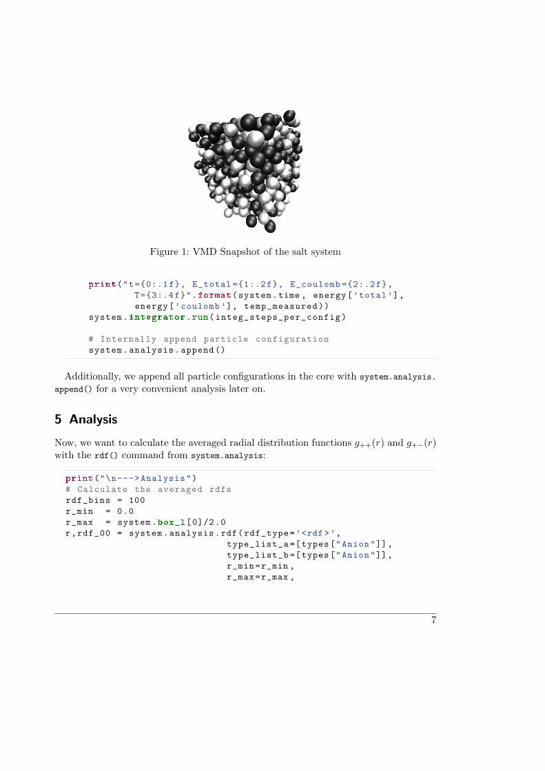
Figure 1: VMD Snapshot of the salt system




system.integrator.run(integ_steps_per_config)

# Internally append particle configuration

system.analysis.append ()

Additionally, we append all particle configurations in the core with system.analysis.

append() for a very convenient analysis later on.

5 Analysis

Now, we want to calculate the averaged radial distribution functions g++(r) and g+−(r)with the rdf() command from system.analysis:

print("\n--->Analysis")

# Calculate the averaged rdfs

rdf_bins = 100

r_min = 0.0

r_max = system.box_l[0]/2.0

r,rdf_00 = system.analysis.rdf(rdf_type=’<rdf >’,

type_list_a =[types["Anion"]],

type_list_b =[types["Anion"]],

r_min=r_min ,

r_max=r_max ,

7

0

0.5

1

1.5

2

2.5

3

3.5

4

1 1.5 2 2.5 3

g(r)

r

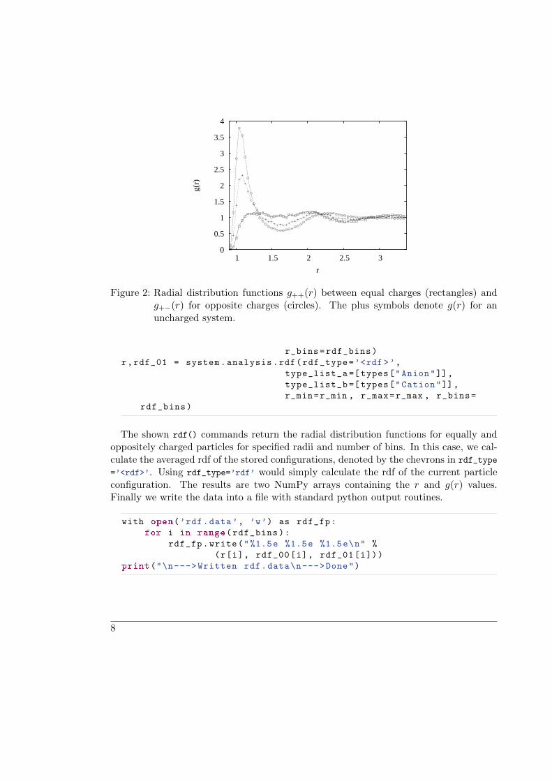
Figure 2: Radial distribution functions g++(r) between equal charges (rectangles) andg+−(r) for opposite charges (circles). The plus symbols denote g(r) for anuncharged system.

r_bins=rdf_bins)

r,rdf_01 = system.analysis.rdf(rdf_type=’<rdf >’,

type_list_a =[types["Anion"]],

type_list_b =[types["Cation"]],

r_min=r_min , r_max=r_max , r_bins=

rdf_bins)

The shown rdf() commands return the radial distribution functions for equally andoppositely charged particles for specified radii and number of bins. In this case, we cal-culate the averaged rdf of the stored configurations, denoted by the chevrons in rdf_type

=’<rdf>’. Using rdf_type=’rdf’ would simply calculate the rdf of the current particleconfiguration. The results are two NumPy arrays containing the r and g(r) values.Finally we write the data into a file with standard python output routines.

with open(’rdf.data’, ’w’) as rdf_fp:

for i in range(rdf_bins):

rdf_fp.write("%1.5e %1.5e %1.5e\n" %

(r[i], rdf_00[i], rdf_01[i]))

print("\n--->Written rdf.data\n--->Done")

8

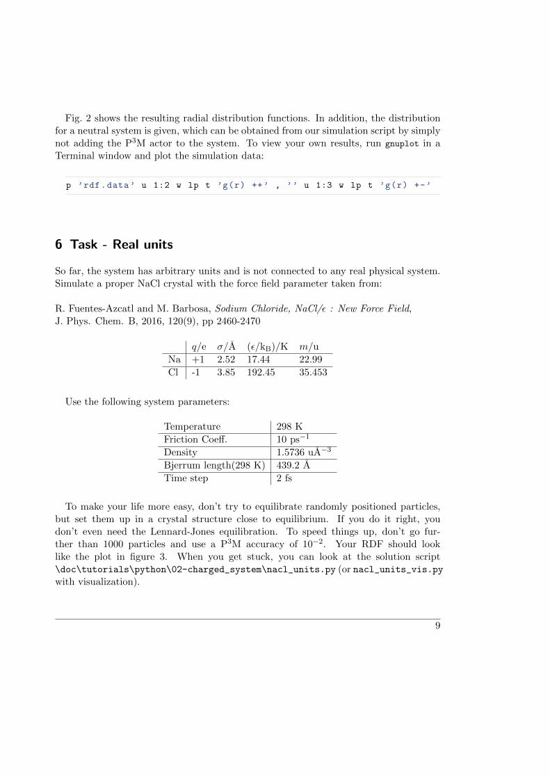
Fig. 2 shows the resulting radial distribution functions. In addition, the distributionfor a neutral system is given, which can be obtained from our simulation script by simplynot adding the P3M actor to the system. To view your own results, run gnuplot in aTerminal window and plot the simulation data:

p ’rdf.data’ u 1:2 w lp t ’g(r) ++’ , ’’ u 1:3 w lp t ’g(r) +-’

6 Task - Real units

So far, the system has arbitrary units and is not connected to any real physical system.Simulate a proper NaCl crystal with the force field parameter taken from:

R. Fuentes-Azcatl and M. Barbosa, Sodium Chloride, NaCl/ε : New Force Field,J. Phys. Chem. B, 2016, 120(9), pp 2460-2470

q/e σ/A (ε/kB)/K m/u

Na +1 2.52 17.44 22.99

Cl -1 3.85 192.45 35.453

Use the following system parameters:

Temperature 298 K

Friction Coeff. 10 ps−1

Density 1.5736 uA−3

Bjerrum length(298 K) 439.2 A

Time step 2 fs

To make your life more easy, don’t try to equilibrate randomly positioned particles,but set them up in a crystal structure close to equilibrium. If you do it right, youdon’t even need the Lennard-Jones equilibration. To speed things up, don’t go fur-ther than 1000 particles and use a P3M accuracy of 10−2. Your RDF should looklike the plot in figure 3. When you get stuck, you can look at the solution script\doc\tutorials\python\02-charged_system\nacl_units.py (or nacl_units_vis.pywith visualization).

9

Figure 3: Snapshot and RDF of the parametrized NaCl crystal.

7 2D Electrostatics and Constraints

In this section, we use the parametrized NaCl system from the last task to simulate amolten salt in a parallel plate capacitor with and without applied electric field. We haveto extend our simulation by several aspects:

ConfinementESPResSo features a number of basic shapes like cylinders, walls or spheres to simulateconfined systems. Here, we use to walls at z = 0 and z = Lz for the parallel plate setup(Lz: Box length in z-direction).

2D-ElectrostaticsESPResSo also has a number of ways to account for the unwanted electrostatic interac-tion in the now non-periodic z-dimension. We use the 3D-periodic P3M algorithm incombination with the Electrostatic Layer Correction (ELC). ELC subtracts the forcescaused by the periodic images in the z-dimension. Another way would be to use theexplicit 2D-electrostatics algorithm MMM2D, also available in ESPResSo.

Electric FieldThe simple geometry of the system allows us to treat an electric field in z-direction as ahomogeneous force. Note that we use inert walls here and don’t take into account thedielectric contrast caused by metal electrodes.

10

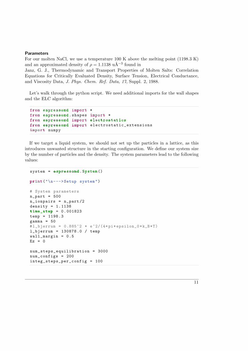
ParametersFor our molten NaCl, we use a temperature 100 K above the melting point (1198.3 K)and an approximated density of ρ = 1.1138 uA−3 found inJanz, G. J., Thermodynamic and Transport Properties of Molten Salts: CorrelationEquations for Critically Evaluated Density, Surface Tension, Electrical Conductance,and Viscosity Data, J. Phys. Chem. Ref. Data, 17, Suppl. 2, 1988.

Let’s walk through the python script. We need additional imports for the wall shapesand the ELC algorithm:

from espressomd import *

from espressomd.shapes import *

from espressomd import electrostatics

from espressomd import electrostatic_extensions

import numpy

If we target a liquid system, we should not set up the particles in a lattice, as thisintroduces unwanted structure in the starting configuration. We define our system sizeby the number of particles and the density. The system parameters lead to the followingvalues:

system = espressomd.System()

print("\n--->Setup system")

# System parameters

n_part = 500

n_ionpairs = n_part /2

density = 1.1138

time_step = 0.001823

temp = 1198.3

gamma = 50

#l_bjerrum = 0.885^2 * e^2/(4* pi*epsilon_0*k_B*T)

l_bjerrum = 130878.0 / temp

wall_margin = 0.5

Ez = 0

num_steps_equilibration = 3000

num_configs = 200

integ_steps_per_config = 100

11

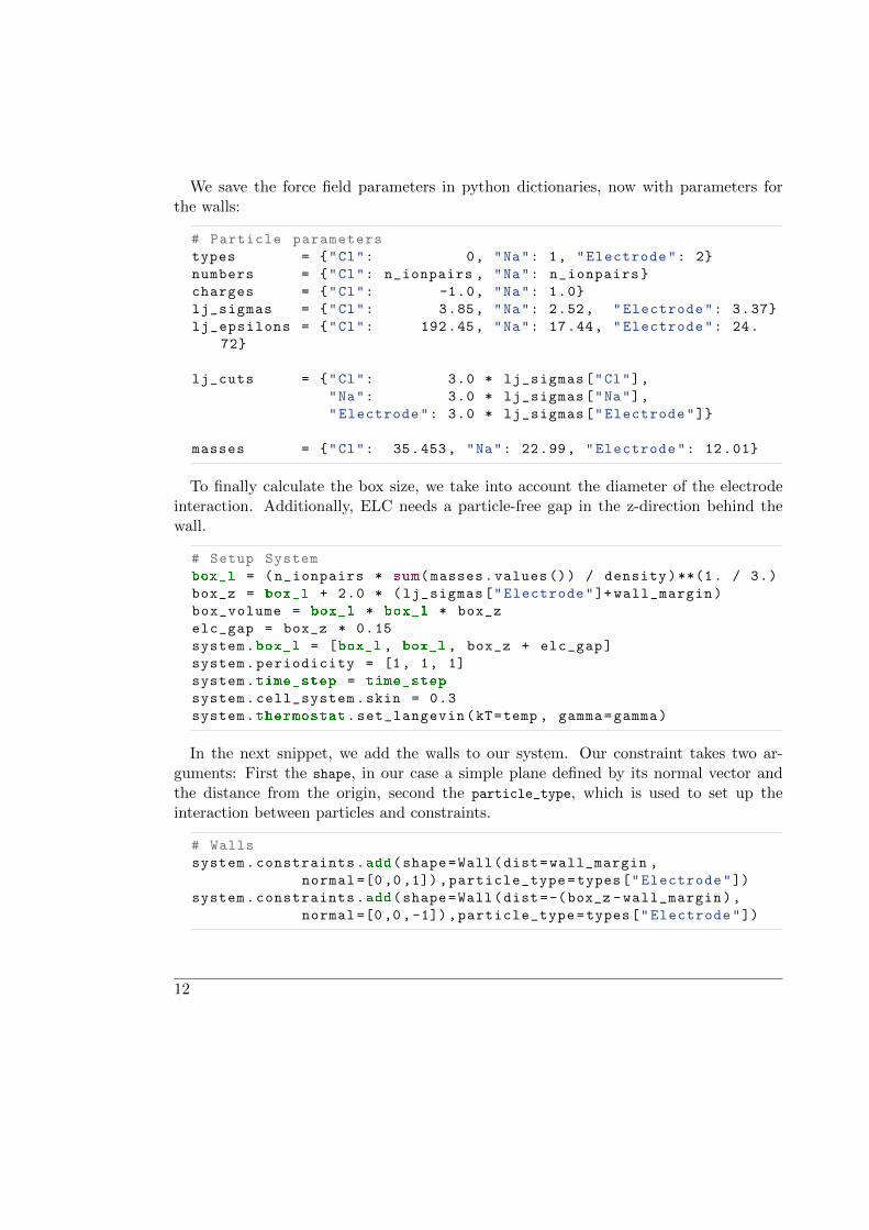
We save the force field parameters in python dictionaries, now with parameters forthe walls:

# Particle parameters

types = {"Cl": 0, "Na": 1, "Electrode": 2}

numbers = {"Cl": n_ionpairs , "Na": n_ionpairs}

charges = {"Cl": -1.0, "Na": 1.0}

lj_sigmas = {"Cl": 3.85, "Na": 2.52, "Electrode": 3.37}

lj_epsilons = {"Cl": 192.45, "Na": 17.44, "Electrode": 24.

72}

lj_cuts = {"Cl": 3.0 * lj_sigmas["Cl"],

"Na": 3.0 * lj_sigmas["Na"],

"Electrode": 3.0 * lj_sigmas["Electrode"]}

masses = {"Cl": 35.453, "Na": 22.99, "Electrode": 12.01}

To finally calculate the box size, we take into account the diameter of the electrodeinteraction. Additionally, ELC needs a particle-free gap in the z-direction behind thewall.

# Setup System

box_l = (n_ionpairs * sum(masses.values ()) / density)**(1. / 3.)

box_z = box_l + 2.0 * (lj_sigmas["Electrode"]+ wall_margin)

box_volume = box_l * box_l * box_z

elc_gap = box_z * 0.15

system.box_l = [box_l , box_l , box_z + elc_gap]

system.periodicity = [1, 1, 1]

system.time_step = time_step

system.cell_system.skin = 0.3


In the next snippet, we add the walls to our system. Our constraint takes two ar-guments: First the shape, in our case a simple plane defined by its normal vector andthe distance from the origin, second the particle_type, which is used to set up theinteraction between particles and constraints.

# Walls

system.constraints.add(shape=Wall(dist=wall_margin ,

normal =[0 ,0 ,1]),particle_type=types["Electrode"])

system.constraints.add(shape=Wall(dist=-(box_z -wall_margin),

normal =[0,0,-1]),particle_type=types["Electrode"])

12

Now we place the particles at random position without overlap with the walls:

# Place particles


p = numpy.random.random (3)*box_l

p[2] += lj_sigmas["Electrode"]

system.part.add(id=len(system.part), type=types["Cl"], pos=

p, q=charges["Cl"], mass=masses["Cl"])


p = numpy.random.random (3)*box_l

p[2] += lj_sigmas["Electrode"]

system.part.add(id=len(system.part), type=types["Na"], pos=

p, q=charges["Na"], mass=masses["Na"])

The scheme to set up the Lennard-Jones interaction is the same as before, extendedby the Electrode-Ion interactions:

# Lennard -Jones interactions parameters

def combination_rule_epsilon(rule , eps1 , eps2):

if rule=="Lorentz":

return (eps1*eps2)**0.5

else:


def combination_rule_sigma(rule , sig1 , sig2):

if rule=="Berthelot":

return (sig1+sig2)*0.5

else:


for s in [["Cl", "Na"], ["Cl", "Cl"], ["Na", "Na"], ["Na", "

Electrode"], ["Cl", "Electrode"]]:

lj_sig = combination_rule_sigma("Berthelot",

lj_sigmas[s[0]], lj_sigmas[s[1]])

lj_cut = combination_rule_sigma("Berthelot",

lj_cuts[s[0]], lj_cuts[s[1]])

lj_eps = combination_rule_epsilon("Lorentz",

lj_epsilons[s[0]], lj_epsilons[s[1]])

system.non_bonded_inter[types[s[0]], types[s[1]]].

lennard_jones.set_params(epsilon=lj_eps ,

13

sigma=lj_sig , cutoff=lj_cut , shift="auto")

Next is the Lennard-Jones Equilibration. Here we use an alternative way to get rid ofthe overlap: ESPResSo features a routine for energy minimization with similar featuresas in the manual implementation used before. Basically it caps the forces and limits thedisplacement during integration.


print "Before Minimization: E_total=", energy[’total ’]

system.minimize_energy.init(f_max = 10, gamma = 10.0,

max_steps = 1000, max_displacement= 0.2)

system.minimize_energy.minimize ()


print "After Minimization: E_total=", energy[’total ’]

As described, we use P3M in combination with ELC to account for the 2D-periodicity.ELC is also added to the actors of the system and takes gap size and maximum pairwiseerrors as arguments.

print("\n--->Tuning Electrostatics")

p3m = electrostatics.P3M(bjerrum_length=l_bjerrum ,

accuracy=1e-2)

system.actors.add(p3m)

elc = electrostatic_extensions.ELC(gap_size = elc_gap ,

maxPWerror = 1e-3)

system.actors.add(elc)

For now, our electric field is zero, but we want to switch it on later. Here we run overall particles and set an external force on the charges caused by the field:

for p in system.part:

p.ext_force = [0,0,Ez * p.q]

This is followed by our standard temperature equilibration:

print("\n--->Temperature Equilibration")

system.time = 0.0

for i in range(num_steps_equilibration /100):



14





In the integration loop, we like to measure the density profile for both ion speciesalong the z-direction. We use a simple histogram analysis to accumulate the densitydata.

print("\n--->Integration")

bins =100

z_dens_na = numpy.zeros(bins)

z_dens_cl = numpy.zeros(bins)

system.time = 0.0

cnt = 0

for i in range(num_configs):






system.integrator.run(integ_steps_per_config)

for p in system.part:

bz = int(p.pos[2]/ box_z*bins)

if p.type == types["Na"]:

z_dens_na[bz] += 1.0

elif p.type == types["Cl"]:

z_dens_cl[bz] += 1.0

cnt += 1

Finally, we calculate the average, normalize the data with the bin volume and save itto a file using NumPy’s savetxt command.

print("\n--->Analysis")

#Average / Normalize with Volume

z_dens_na /= (cnt * box_volume/bins)

z_dens_cl /= (cnt * box_volume/bins)

z_values = numpy.linspace(0,box_l ,num=bins)

res = numpy.column_stack ((z_values ,z_dens_na ,z_dens_cl))

numpy.savetxt("z_density.data",res ,

15

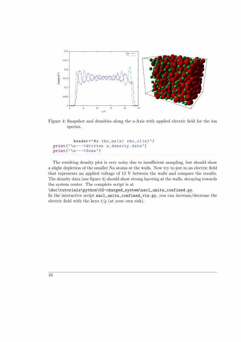
Figure 4: Snapshot and densities along the z-Axis with applied electric field for the ionspecies.

header="#z rho_na(z) rho_cl(z)")

print("\n--->Written z_density.data")

print("\n--->Done")

The resulting density plot is very noisy due to insufficient sampling, but should showa slight depletion of the smaller Na atoms at the walls. Now try to put in an electric fieldthat represents an applied voltage of 15 V between the walls and compare the results.The density data (see figure 4) should show strong layering at the walls, decaying towardsthe system center. The complete script is at\doc\tutorials\python\02-charged_system\nacl_units_confined.py.In the interactive script nacl_units_confined_vis.py, you can increase/decrease theelectric field with the keys t/g (at your own risk).

16

Documents

Tutorial 2: A simple charged system - ESPResSoespressomd.org/wordpress/wp-content/uploads/2016/10/02-charged... · Tutorial 2: A simple charged system October 9, 2016 Contents 1 Introduction