Embed Size (px)
Citation preview

Tutorial 6
CPSC 340
Overview
• Regularization
• RBF Basis
• Robust Regression
• Gradient descent
1

Regularization
Regularization - Motivation
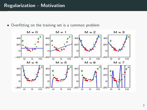
• Overfitting on the training set is a common problem
2
Regularization - Motivation
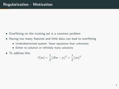
• Overfitting on the training set is a common problem
• Having too many features and little data can lead to overfitting
• Underdetermined system: fewer equations than unknowns
• Either no solution or infinitely many solutions
• To address this:
f (w) =1
2||Xw − y ||2 +
λ
2||w ||2
3
Regularization - Motivation
• Overfitting on the training set is a common problem
• Having too many features and little data can lead to overfitting
• Underdetermined system: fewer equations than unknowns
• Either no solution or infinitely many solutions
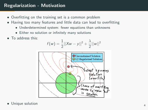
• To address this:
f (w) =1
2||Xw − y ||2 +
λ
2||w ||2
• Unique solution4
Regularization - Motivation
• Overfitting on the training set is a common problem
• Having too many features and little data can lead to overfitting
• Underdetermined system: fewer equations than unknowns
• Either no solution or infinitely many solutions
• To address this:
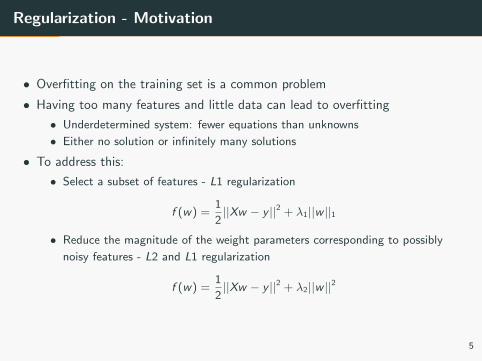
• Select a subset of features - L1 regularization
f (w) =1
2||Xw − y ||2 + λ1||w ||1
• Reduce the magnitude of the weight parameters corresponding to possibly
noisy features - L2 and L1 regularization
f (w) =1
2||Xw − y ||2 + λ2||w ||2
5
Regularization - Motivation
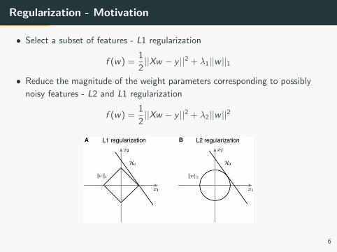
• Select a subset of features - L1 regularization
f (w) =1
2||Xw − y ||2 + λ1||w ||1
• Reduce the magnitude of the weight parameters corresponding to possibly
noisy features - L2 and L1 regularization
f (w) =1
2||Xw − y ||2 + λ2||w ||2
6
Regularization - Definition
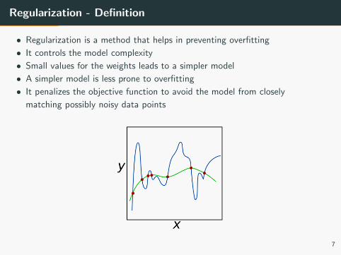
• Regularization is a method that helps in preventing overfitting
• It controls the model complexity
• Small values for the weights leads to a simpler model
• A simpler model is less prone to overfitting
• It penalizes the objective function to avoid the model from closely
matching possibly noisy data points
7
Regularization - Definition
8
Regularization - Exercise
• Consider the following L2 regularized least square objective function
f (w) =1
2||Xw − y ||2 + λ2||w ||2
• How does λ2 affect the decision boundary ?
9
Regularization - Exercise
• Consider the following L2 regularized least square objective function
f (w) =1
2||Xw − y ||2 + λ2||w ||2
• How does λ2 affect the decision boundary ?
• λ2 controls a trade off between fitting the training set well and keeping
the weights small
• Large λ2 can lead to underfitting (a more linear, simple model)
• Small λ2 can lead to overfitting (a more complicated model - larger range
of values for the parameters)
10
Regularization - Exercise
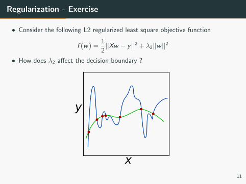
• Consider the following L2 regularized least square objective function
f (w) =1
2||Xw − y ||2 + λ2||w ||2
• How does λ2 affect the decision boundary ?
11
Radial Basis Function
RBF Basis - Motivation
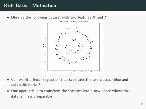
• Observe the following dataset with two features X and Y
• Can we fit a linear regression that seperates the two classes (blue and
red) sufficiently ?
• One approach is to transform the features into a new space where the
data is linearly separable
12
RBF Basis
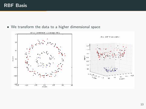
• We transform the data to a higher dimensional space
13
RBF Basis
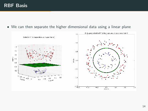
• We can then separate the higher dimensional data using a linear plane
14
RBF Basis
• Given X ∈ RN×D , transform X to Z ∈ RN×N where
Zij = exp(−||Xi − Xj ||2
2σ2)
where σ controls the influence of nearby points
• Intuitively, Zij is a similarity value between sample i and sample j
15
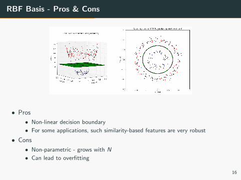
RBF Basis - Pros & Cons
• Pros
• Non-linear decision boundary
• For some applications, such similarity-based features are very robust
• Cons
• Non-parametric - grows with N
• Can lead to overfitting
16
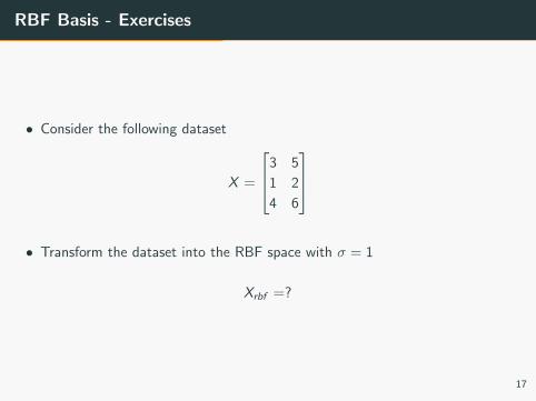
RBF Basis - Exercises
• Consider the following dataset
X =
3 5
1 2
4 6
• Transform the dataset into the RBF space with σ = 1
Xrbf =?
17
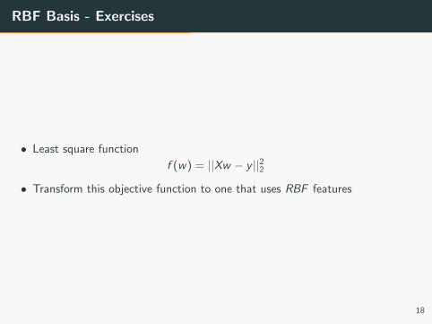
RBF Basis - Exercises
• Least square function
f (w) = ||Xw − y ||22
• Transform this objective function to one that uses RBF features
18

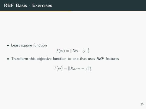
RBF Basis - Exercises
• Least square function
f (w) = ||Xw − y ||22
• Transform this objective function to one that uses RBF features
f (w) = ||Xrbfw − y ||22
19
RBF Basis - Exercises
• Least square function
f (w) = ||Xw − y ||22
• Transform this objective function to one that uses RBF features
f (w) = ||Xrbfw − y ||22
20
RBF Basis - Exercises
• Least square function
f (w) = ||Xw − y ||22
• Transform this objective function to one that uses RBF features
f (w) = ||Xrbfw − y ||22
• Recall that RBF can lead to a model that is too complicated for the
dataset - potentially causing overfitting
• Regularization helps against overfitting
• Add the L1 and L2 regularization terms to f (w)
21
RBF Basis - Exercises
• Least square function
f (w) = ||Xw − y ||22
• Transform this objective function to one that uses RBF features
f (w) = ||Xrbfw − y ||22
• Recall that RBF can lead to a model that is too complicated for the
dataset - potentially causing overfitting
• Regularization helps against overfitting
• Add the L1 and L2 regularization terms to f (w)
f (w) = ||Xrbfw − y ||22 + λ1||w ||1 + λ2||w ||22
• Suggest one way to choose the values for λ1 and λ2
22
RBF Basis - Exercises
• Least square function
f (w) = ||Xw − y ||22
• Transform this objective function to one that uses RBF
frbf (w) = ||Xrbfw − y ||22
• Recall that RBF can lead to a model that is too complicated for the
dataset - potentially causing overfitting
• Regularization helps against overfitting
• Add the L1 and L2 regularization terms to f (w)
frbf (w) = ||Xrbfw − y ||22 + λ1||w ||1 + λ2||w ||22
• How do we choose the values for λ1 and λ2 ?
23
RBF Basis - Exercises
• Least square function
f (w) = ||Xw − y ||22
• Transform this objective function to one that uses RBF
frbf (w) = ||Xrbfw − y ||22
• Recall that RBF can lead to a model that is too complicated for the
dataset - potentially causing overfitting
• Regularization helps against overfitting
• Add the L1 and L2 regularization terms to f (w)
frbf (w) = ||Xrbfw − y ||22 + λ1||w ||1 + λ2||w ||22
• How do we choose the values for λ1 and λ2 ?
• Cross-validation
24
RBF Basis - Exercises
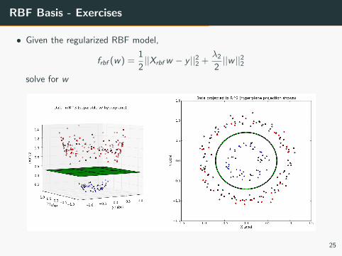
• Given the regularized RBF model,
frbf (w) =1
2||Xrbfw − y ||22 +
λ22||w ||22
solve for w
25
RBF Basis - Exercises
• Given the regularized RBF model,
frbf (w) =1
2||Xrbfw − y ||22 +
λ22||w ||22
solve for w
26
RBF Basis - Exercises
• Given the regularized RBF model,
frbf (w) =1
2||Xrbfw − y ||22 +
λ22||w ||22
solve for w
w = (XTrbf Xrbf + Iλ2)−1XT
rbf y
27

Robust Regression
Weighted Least-Squares
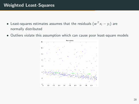
• Least-squares estimates assumes that the residuals (wT xi − yi ) are
normally distributed
• Outliers violate this assumption which can cause poor least-square models
28
Weighted Least-Squares
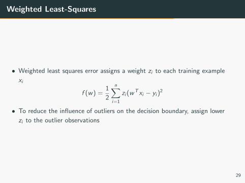
• Weighted least squares error assigns a weight zi to each training example
xi
f (w) =1
2
n∑i=1
zi (wT xi − yi )
2
• To reduce the influence of outliers on the decision boundary, assign lower
zi to the outlier observations
29
Weighted Least-Squares
• To compute w that minimizes f (w) we need to derive the partial
derivatives of f (w) w.r.t each wj and update wj using gradient descent
• Given the one-dimensional weighted least square error function
f (w) =1
2
n∑i=1
zi (wxi − yi )2
derive ∂f (w)∂w
30
Weighted Least-Squares
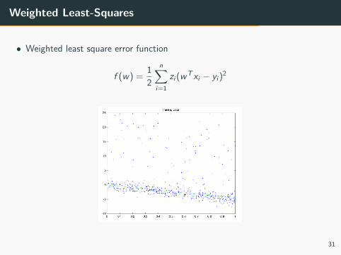
• Weighted least square error function
f (w) =1
2
n∑i=1
zi (wT xi − yi )
2
31
Robust regression - lasso
• Problem: weighted least squares requires us to know the identity of the
outliers
• We can change the least square error function
f (w) =1
2
n∑i=1
(wT xi − yi )2
to the L1-norm error function that is robust to outliers
f (w) =n∑
i=1
|yi − wT xi |
32
Robust regression - lasso
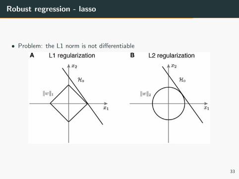
• Problem: the L1 norm is not differentiable
33
Robust regression - lasso
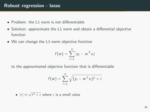
• Problem: the L1 norm is not differentiable
• Solution: approximate the L1 norm and obtain a differential objective
function
• We can change the L1-norm objective function
f (w) =n∑
i=1
|yi − wT xi |
to the approximated objective function that is differentiable
f (w) =n∑
i=1
√(yi − wT xi )2 + ε
• |r | ≈√r 2 + ε where ε is a small value
34
Robust Regression - Exercise
• Given the approximation
f (w) =n∑
i=1
√(yi − wT xi )2 + ε
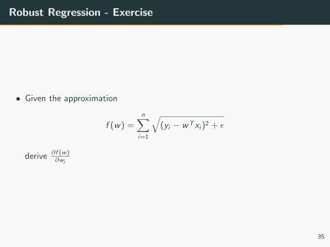
derive ∂f (w)∂wj
35
Robust Regression - Exercise
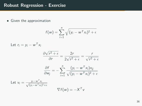
• Given the approximation
f (w) =n∑
i=1
√(yi − wT xi )2 + ε
Let ri = yi − wT xi
∂√r2 + ε
∂r=
2r
2√r2 + ε
=r√
r2 + ε
∂f
∂wj= −
n∑i=1
(yi − wT xi )xij√(yi − wT xi )2 + ε
Let vi = yi−wT xi√(yi−wT xi )2+ε
∇f (w) = −XT v
36

Gradient Descent with minFunc
Gradient Descent
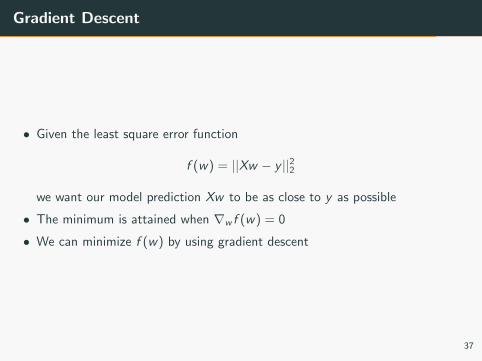
• Given the least square error function
f (w) = ||Xw − y ||22
we want our model prediction Xw to be as close to y as possible
• The minimum is attained when ∇w f (w) = 0
• We can minimize f (w) by using gradient descent
37
Gradient Descent
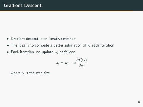
• Gradient descent is an iterative method
• The idea is to compute a better estimation of w each iteration
• Each iteration, we update wi as follows
wi = wi − α∂f (w)
∂wi
where α is the step size
38
Gradient Descent
39
Gradient Descent
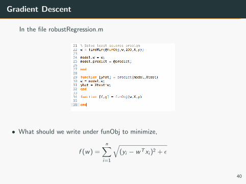
In the file robustRegression.m
• What should we write under funObj to minimize,
f (w) =n∑
i=1
√(yi − wT xi )2 + ε
40
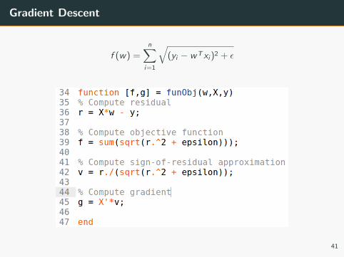
Gradient Descent
f (w) =n∑
i=1
√(yi − wT xi )2 + ε
41