Embed Size (px)
Citation preview
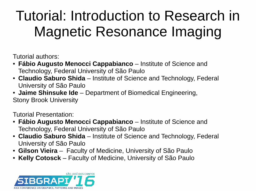
Tutorial: Introduction to Research in Magnetic Resonance Imaging
Tutorial authors: ● Fábio Augusto Menocci Cappabianco – Institute of Science and
Technology, Federal University of São Paulo● Claudio Saburo Shida – Institute of Science and Technology, Federal
University of São Paulo● Jaime Shinsuke Ide – Department of Biomedical Engineering,Stony Brook University
Tutorial Presentation:● Fábio Augusto Menocci Cappabianco – Institute of Science and
Technology, Federal University of São Paulo● Claudio Saburo Shida – Institute of Science and Technology, Federal
University of São Paulo● Gilson Vieira – Faculty of Medicine, University of São Paulo● Kelly Cotosck – Faculty of Medicine, University of São Paulo

Overview
Part I: Magnetic Resonance Image Acquisition – Cláudio Subaro Shida – Pages 3-49
Part II: Magnetic Resonance Image Processing and Analysis – Fábio Augusto Menocci Cappabianco – Page 50-96
Part III: Magnetic Resonance Image Spatial Normalization – Cláudio Subaro Shida – Page 97-120
Part IV: Functional Magnetic Resonance Image Acquisition and Analysis – Gilson Vieira and Kelly Cotosck – Page 121-138
Magnetic Resonance Imaging (MRI)
Sibigrapi 16 – São José dos Campos
2016
Claudio Shida
Email: [email protected]
Aquisition
Summary
- Introduction to MRI
- MRI scanner
- NMR phenomenon
- Relaxation timesT1 and T2
- Image formation: Spin-echo technique (TR and TE)
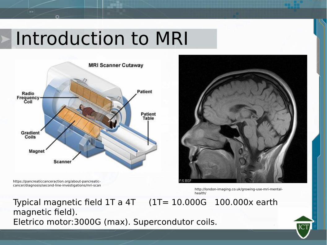
Introduction to MRI
Typical magnetic field 1T a 4T (1T= 10.000G 100.000x earth magnetic field). Eletrico motor:3000G (max). Supercondutor coils.
https://pancreaticcanceraction.org/about-pancreatic-cancer/diagnosis/second-line-investigations/mri-scan/
http://london-imaging.co.uk/growing-use-mri-mental-health/
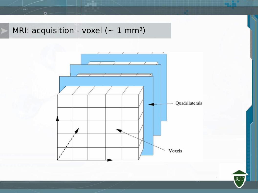
MRI: acquisition - voxel (~ 1 mm3)
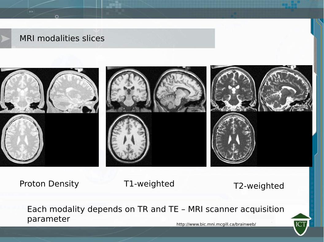
MRI modalities slices
Proton Density T1-weighted T2-weighted
Each modality depends on TR and TE – MRI scanner acquisition parameter
http://www.bic.mni.mcgill.ca/brainweb/
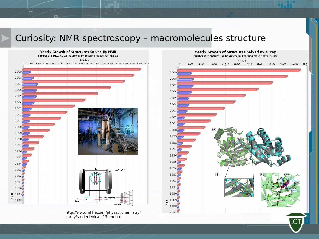
Curiosity: NMR spectroscopy – macromolecules structure
http://www.mhhe.com/physsci/chemistry/carey/student/olc/ch13nmr.html
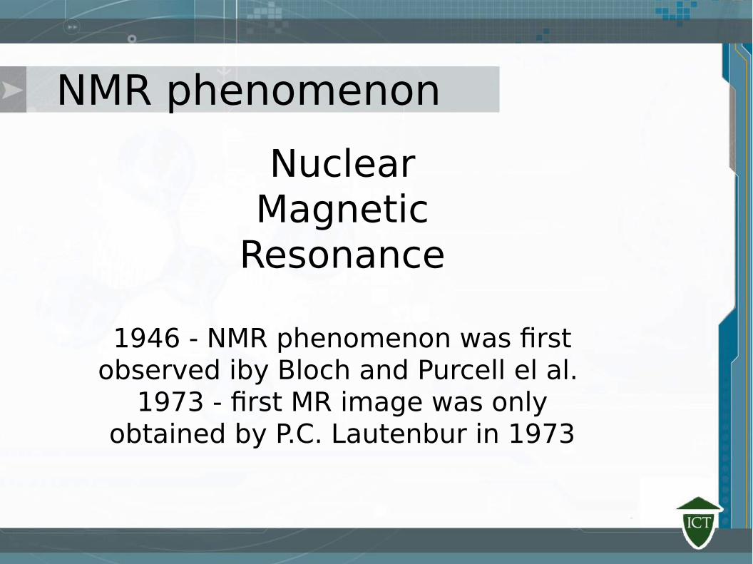
NMR phenomenon
NuclearMagnetic
Resonance
1946 - NMR phenomenon was first observed iby Bloch and Purcell el al.
1973 - first MR image was only obtained by P.C. Lautenbur in 1973
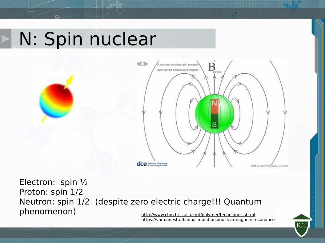
N: Spin nuclear
Electron: spin ½Proton: spin 1/2Neutron: spin 1/2 (despite zero electric charge!!! Quantum phenomenon) http://www.chm.bris.ac.uk/pt/polymer/techniques.shtml
https://vam.anest.ufl.edu/simulations/nuclearmagneticresonance
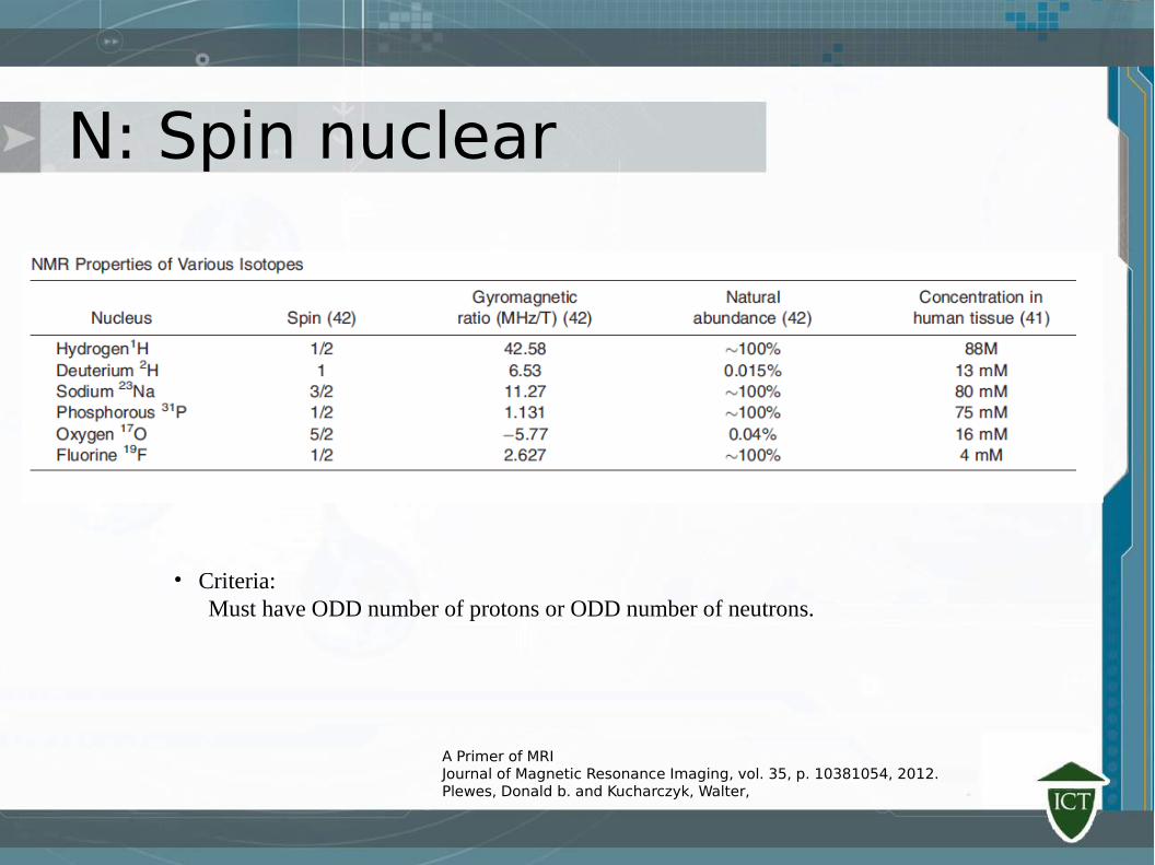
N: Spin nuclear
• Criteria: Must have ODD number of protons or ODD number of neutrons.
A Primer of MRIJournal of Magnetic Resonance Imaging, vol. 35, p. 10381054, 2012.Plewes, Donald b. and Kucharczyk, Walter,
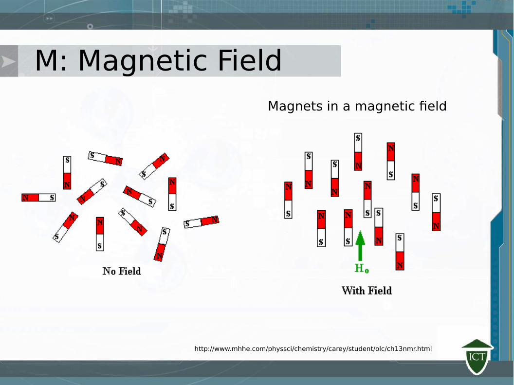
M: Magnetic FieldMagnets in a magnetic field
http://www.mhhe.com/physsci/chemistry/carey/student/olc/ch13nmr.html
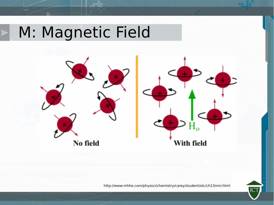
M: Magnetic Field
http://www.mhhe.com/physsci/chemistry/carey/student/olc/ch13nmr.html
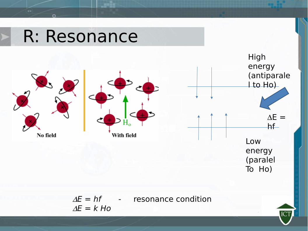
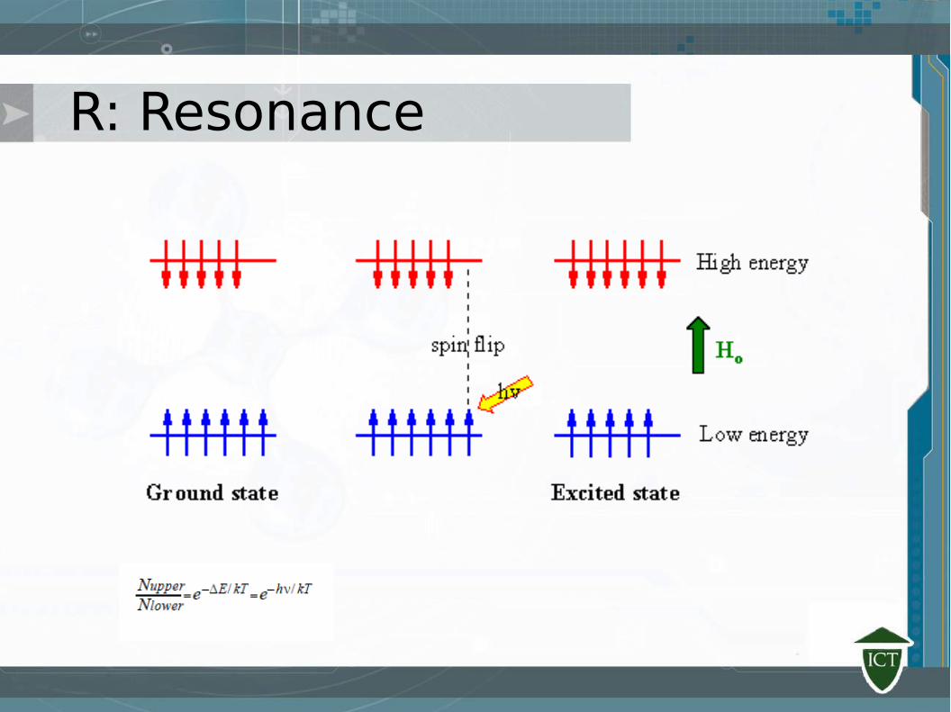
R: Resonance
Low energy(paralelTo Ho)
High energy(antiparalel to Ho)
E = hf
E = hf - resonance conditionE = k Ho
R: Resonance
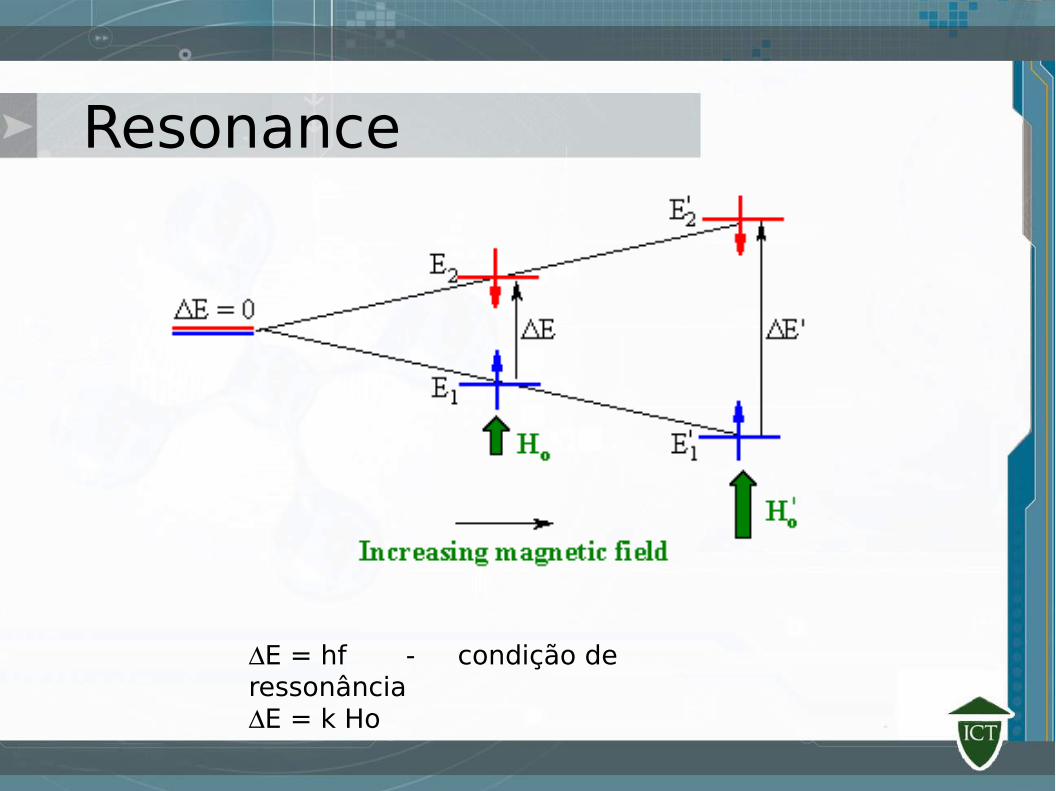
Resonance
E = hf - condição de ressonânciaE = k Ho
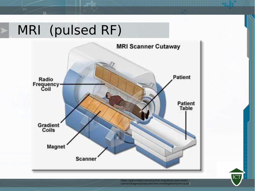
MRI (pulsed RF)
https://pancreaticcanceraction.org/about-pancreatic-cancer/diagnosis/second-line-investigations/mri-scan/
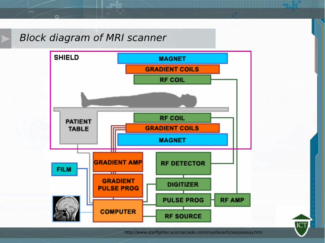
Block diagram of MRI scanner
http://www.starfighter.acornarcade.com/mysite/articles/aiessay.htm

Precession of Nuclear spin in a magnetic field
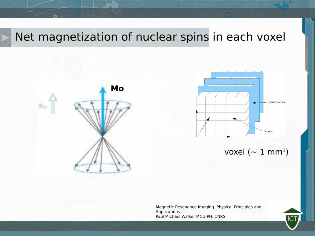
Net magnetization of nuclear spins in each voxel
voxel (~ 1 mm3)
Mo
Magnetic Resonance Imaging. Physical Principles and ApplicationsPaul Michael Walker MCU-PH, CNRS
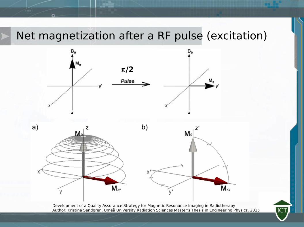
Net magnetization after a RF pulse (excitation)
/2
Development of a Quality Assurance Strategy for Magnetic Resonance Imaging in RadiotherapyAuthor: Kristina Sandgren, Umeå University Radiation Sciences Master’s Thesis in Engineering Physics, 2015
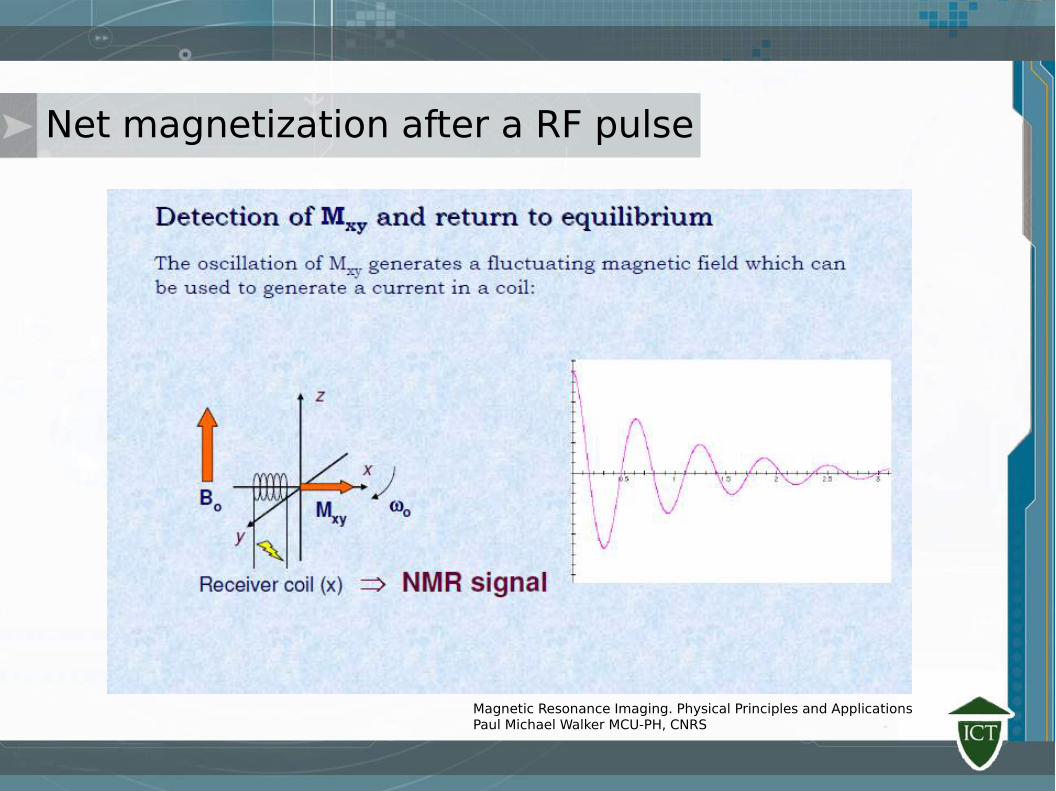
Net magnetization after a RF pulse
Magnetic Resonance Imaging. Physical Principles and ApplicationsPaul Michael Walker MCU-PH, CNRS
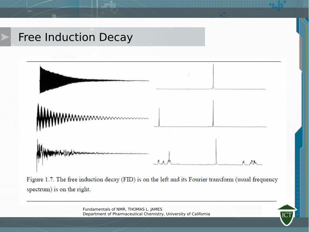
Free Induction Decay
Fundamentals of NMR, THOMAS L. JAMESDepartment of Pharmaceutical Chemistry, University of California
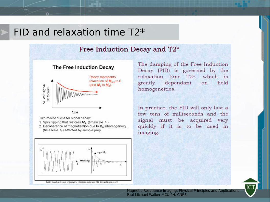
FID and relaxation time T2*
Magnetic Resonance Imaging. Physical Principles and ApplicationsPaul Michael Walker MCU-PH, CNRS
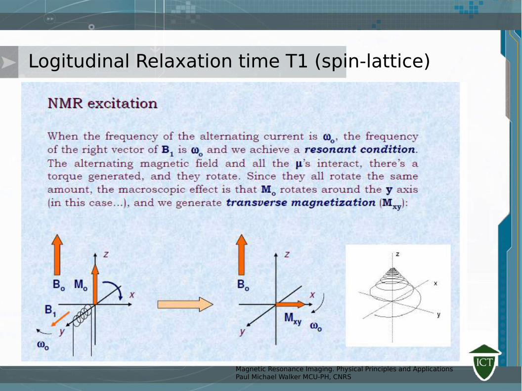
Logitudinal Relaxation time T1 (spin-lattice)
Magnetic Resonance Imaging. Physical Principles and ApplicationsPaul Michael Walker MCU-PH, CNRS
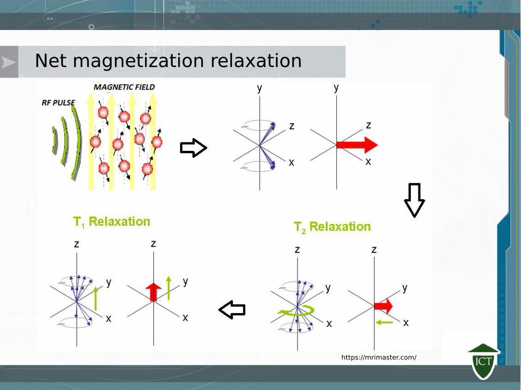
Net magnetization relaxation
https://mrimaster.com/
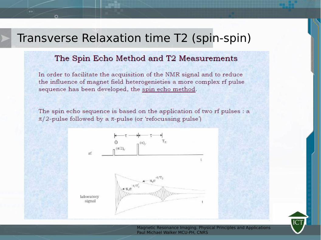
Transverse Relaxation time T2 (spin-spin)
Magnetic Resonance Imaging. Physical Principles and ApplicationsPaul Michael Walker MCU-PH, CNRS
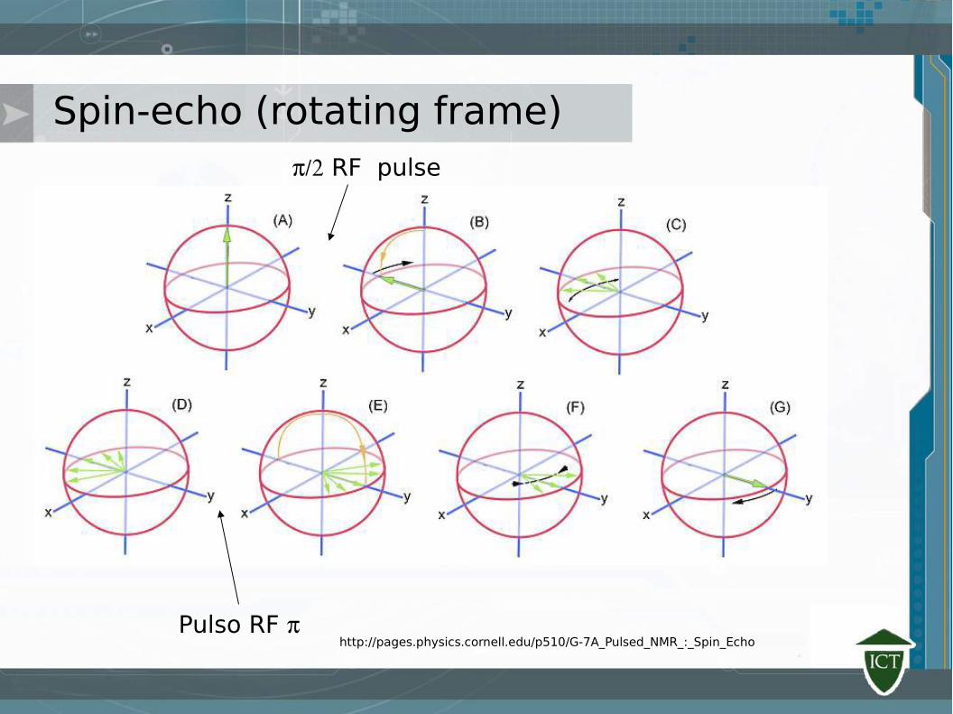
Spin-echo (rotating frame)
Pulso RF
RF pulse
http://pages.physics.cornell.edu/p510/G-7A_Pulsed_NMR_:_Spin_Echo
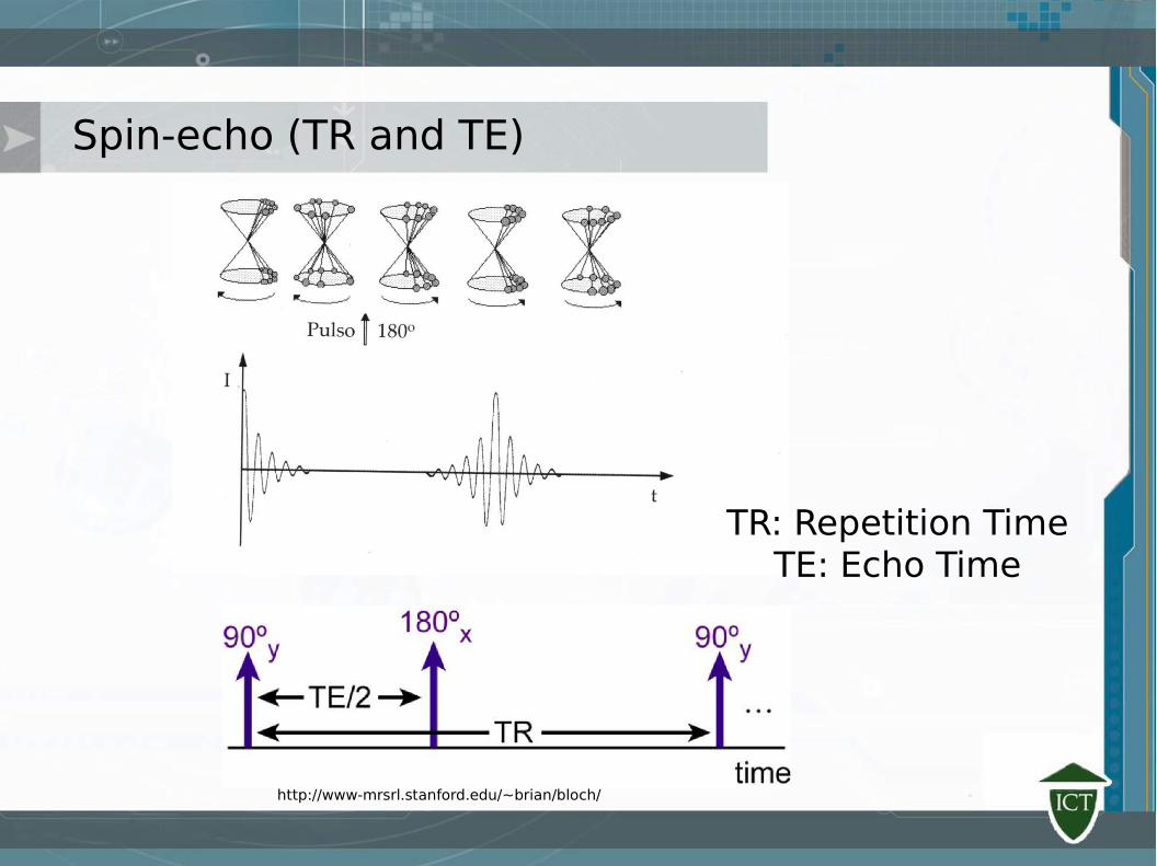
Spin-echo (TR and TE)
TR: Repetition TimeTE: Echo Time
http://www-mrsrl.stanford.edu/~brian/bloch/
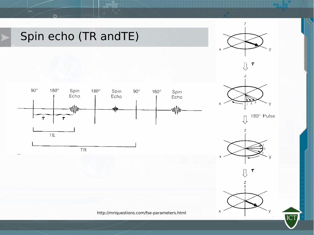
Spin echo (TR andTE)
http://mriquestions.com/fse-parameters.html
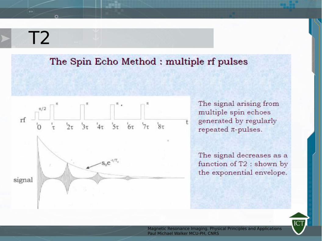
T2
Magnetic Resonance Imaging. Physical Principles and ApplicationsPaul Michael Walker MCU-PH, CNRS
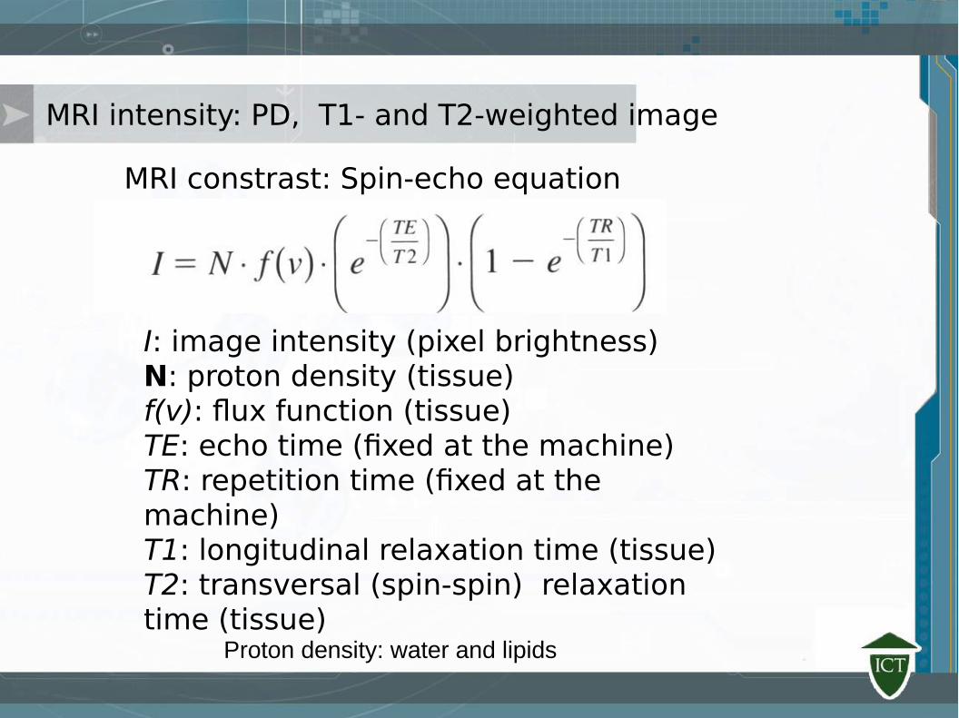
MRI intensity: PD, T1- and T2-weighted image
Proton density: water and lipids
MRI constrast: Spin-echo equation
I: image intensity (pixel brightness)N: proton density (tissue)f(v): flux function (tissue)TE: echo time (fixed at the machine)TR: repetition time (fixed at the machine)T1: longitudinal relaxation time (tissue)T2: transversal (spin-spin) relaxation time (tissue)
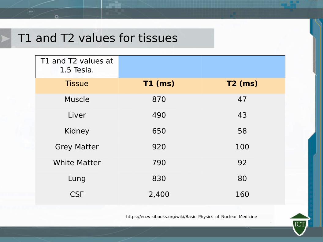
T1 and T2 values for tissues
T1 and T2 values at 1.5 Tesla.
Tissue T1 (ms) T2 (ms)
Muscle 870 47
Liver 490 43
Kidney 650 58
Grey Matter 920 100
White Matter 790 92
Lung 830 80
CSF 2,400 160
https://en.wikibooks.org/wiki/Basic_Physics_of_Nuclear_Medicine
http://mriquestions.com/image-contrast-trte.html
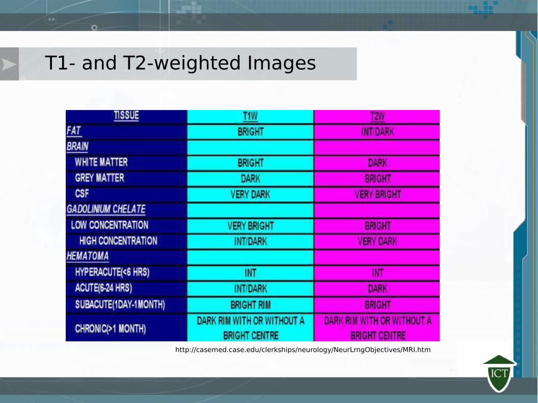
T1- and T2-weighted Images
http://casemed.case.edu/clerkships/neurology/NeurLrngObjectives/MRI.htm
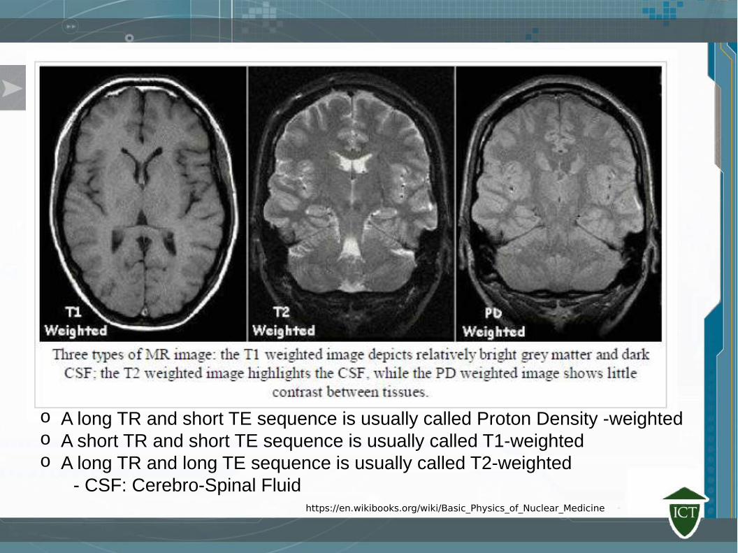
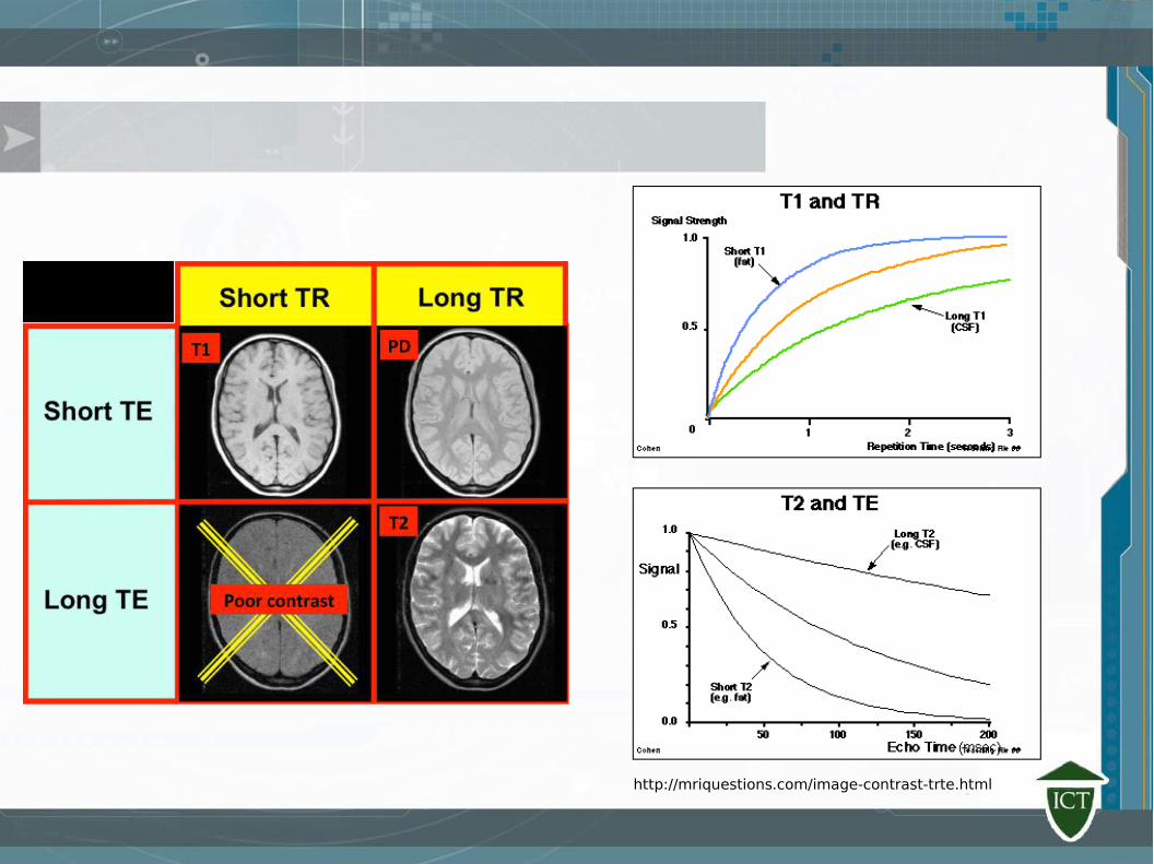
o A long TR and short TE sequence is usually called Proton Density -weightedo A short TR and short TE sequence is usually called T1-weightedo A long TR and long TE sequence is usually called T2-weighted
- CSF: Cerebro-Spinal Fluidhttps://en.wikibooks.org/wiki/Basic_Physics_of_Nuclear_Medicine
Image
http://en.wikibooks.org/wiki/Basic_Physics_of_Nuclear_Medicine
Imagem
http://en.wikibooks.org/wiki/Basic_Physics_of_Nuclear_Medicine
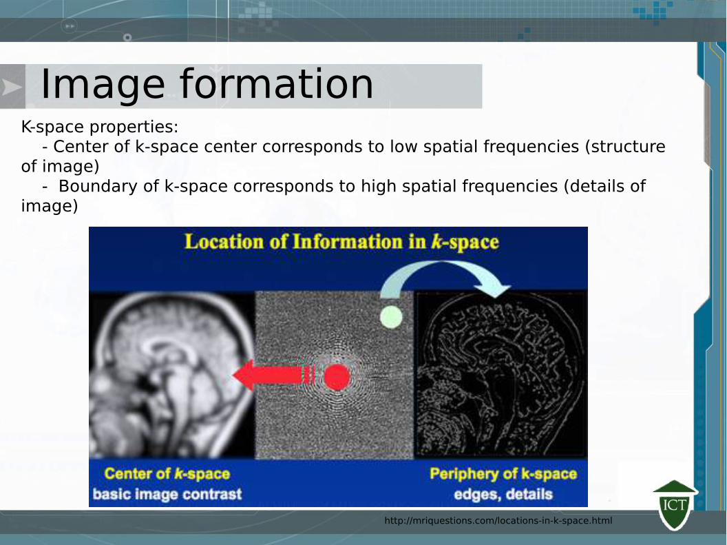
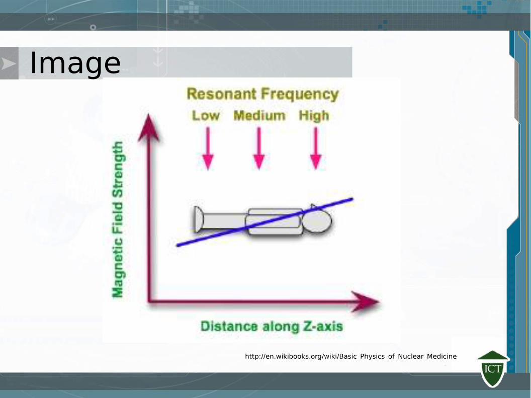
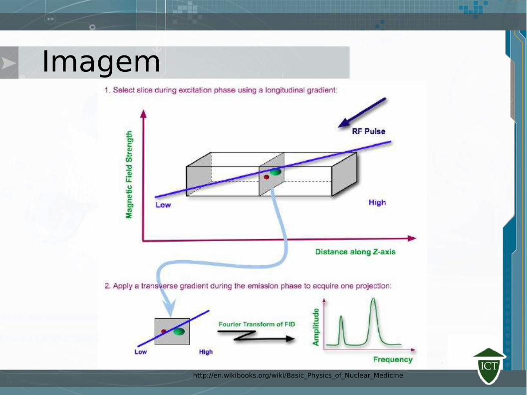
Image formationK-space properties: - Center of k-space center corresponds to low spatial frequencies (structure of image) - Boundary of k-space corresponds to high spatial frequencies (details of image)
http://mriquestions.com/locations-in-k-space.html
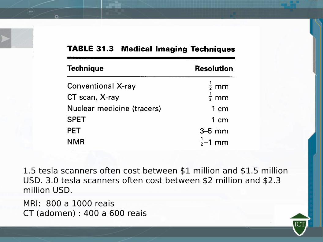
1.5 tesla scanners often cost between $1 million and $1.5 million USD. 3.0 tesla scanners often cost between $2 million and $2.3 million USD.
MRI: 800 a 1000 reaisCT (adomen) : 400 a 600 reais
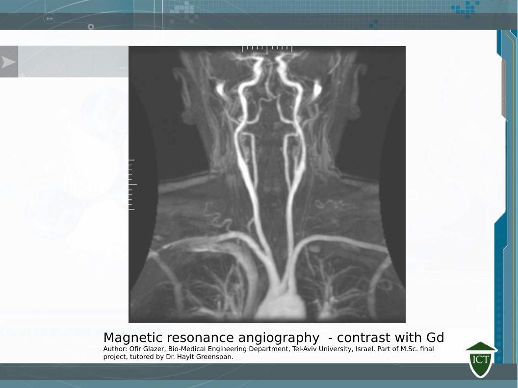
Magnetic resonance angiography - contrast with GdAuthor: Ofir Glazer, Bio-Medical Engineering Department, Tel-Aviv University, Israel. Part of M.Sc. final project, tutored by Dr. Hayit Greenspan.
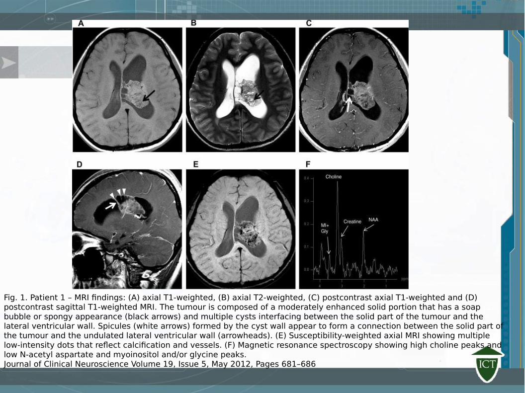
Fig. 1. Patient 1 – MRI findings: (A) axial T1-weighted, (B) axial T2-weighted, (C) postcontrast axial T1-weighted and (D) postcontrast sagittal T1-weighted MRI. The tumour is composed of a moderately enhanced solid portion that has a soap bubble or spongy appearance (black arrows) and multiple cysts interfacing between the solid part of the tumour and the lateral ventricular wall. Spicules (white arrows) formed by the cyst wall appear to form a connection between the solid part of the tumour and the undulated lateral ventricular wall (arrowheads). (E) Susceptibility-weighted axial MRI showing multiple low-intensity dots that reflect calcification and vessels. (F) Magnetic resonance spectroscopy showing high choline peaks and low N-acetyl aspartate and myoinositol and/or glycine peaks.Journal of Clinical Neuroscience Volume 19, Issue 5, May 2012, Pages 681–686
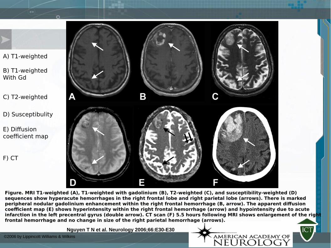
Nguyen T N et al. Neurology 2006;66:E30-E30©2006 by Lippincott Williams & Wilkins
Figure. MRI T1-weighted (A), T1-weighted with gadolinium (B), T2-weighted (C), and susceptibility-weighted (D) sequences show hyperacute hemorrhages in the right frontal lobe and right parietal lobe (arrows). There is marked peripheral nodular gadolinium enhancement within the right frontal hemorrhage (B, arrow). The apparent diffusion coefficient map (E) shows hyperintensity within the right frontal hemorrhage (arrow) and hypointensity due to acute infarction in the left precentral gyrus (double arrow). CT scan (F) 5.5 hours following MRI shows enlargement of the right frontal hemorrhage and no change in size of the right parietal hemorrhage (arrows).
A) T1-weighted
C) T2-weighted
E) Diffusion coefficient map
F) CT
D) Susceptibulity
B) T1-weightedWith Gd
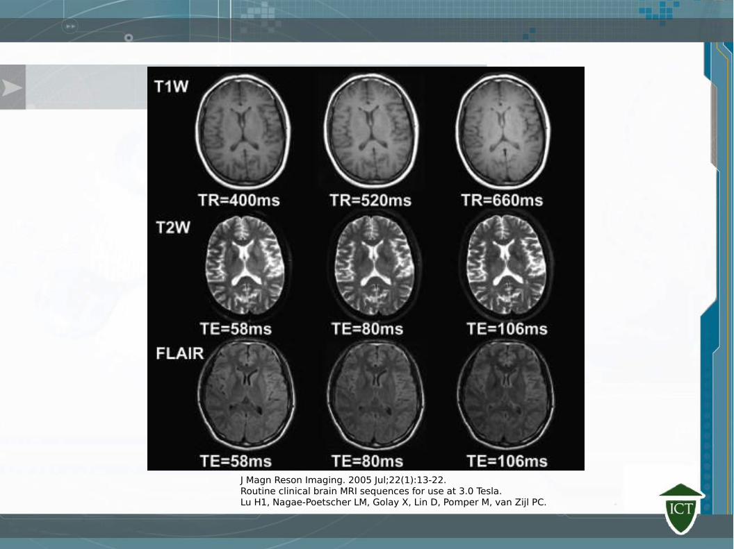
J Magn Reson Imaging. 2005 Jul;22(1):13-22.Routine clinical brain MRI sequences for use at 3.0 Tesla.Lu H1, Nagae-Poetscher LM, Golay X, Lin D, Pomper M, van Zijl PC.
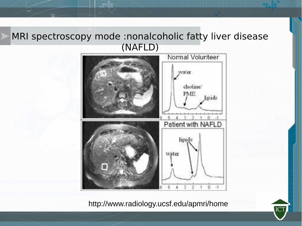
MRI spectroscopy mode :nonalcoholic fatty liver disease (NAFLD)
http://www.radiology.ucsf.edu/apmri/home
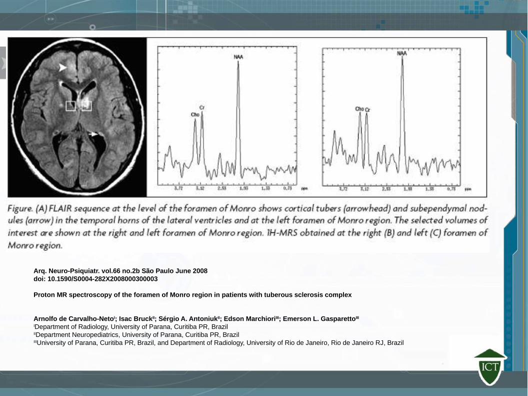
Arq. Neuro-Psiquiatr. vol.66 no.2b São Paulo June 2008doi: 10.1590/S0004-282X2008000300003 Proton MR spectroscopy of the foramen of Monro region in patients with tuberous sclerosis complex
Arnolfo de Carvalho-NetoI; Isac BruckII; Sérgio A. AntoniukII; Edson MarchioriIII; Emerson L. GasparettoIII
IDepartment of Radiology, University of Parana, Curitiba PR, Brazil IIDepartment Neuropediatrics, University of Parana, Curitiba PR, Brazil IIIUniversity of Parana, Curitiba PR, Brazil, and Department of Radiology, University of Rio de Janeiro, Rio de Janeiro RJ, Brazil
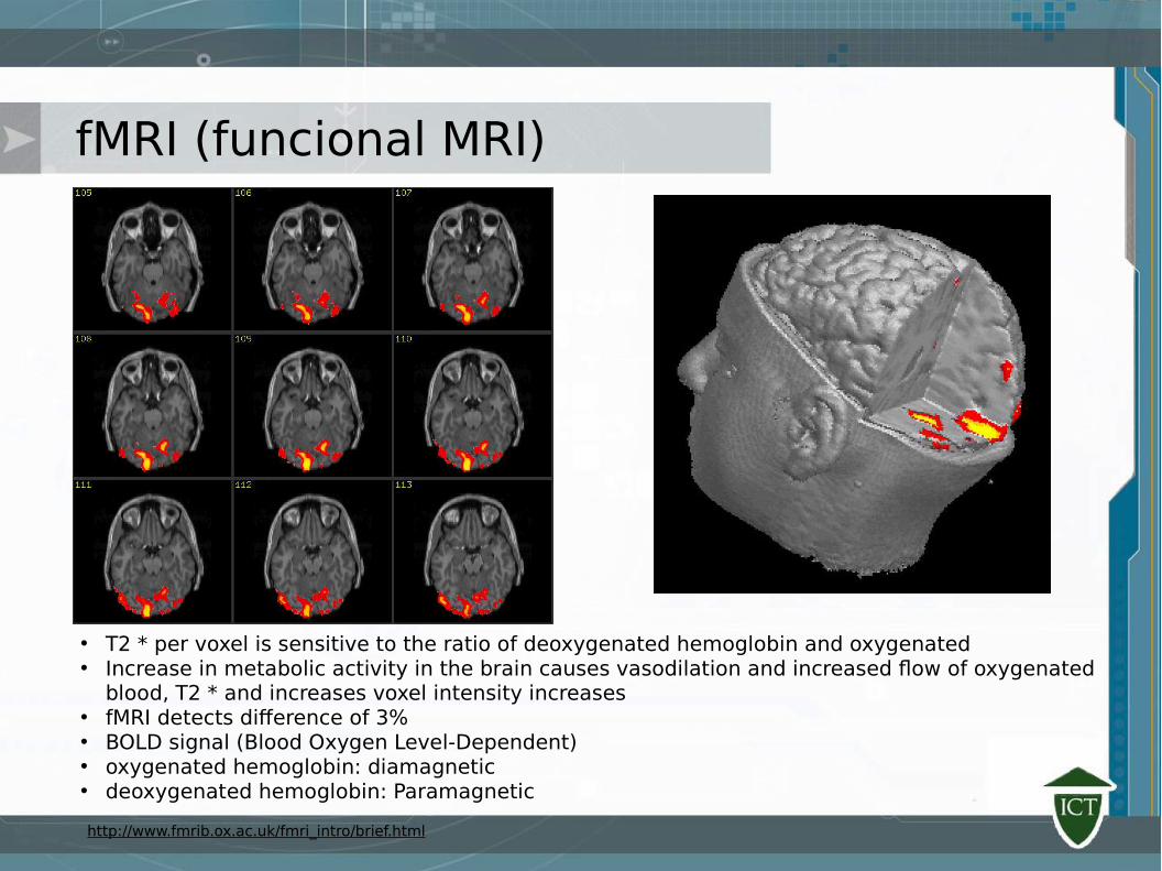
fMRI (funcional MRI)
• T2 * per voxel is sensitive to the ratio of deoxygenated hemoglobin and oxygenated• Increase in metabolic activity in the brain causes vasodilation and increased flow of oxygenated
blood, T2 * and increases voxel intensity increases• fMRI detects difference of 3%• BOLD signal (Blood Oxygen Level-Dependent)• oxygenated hemoglobin: diamagnetic• deoxygenated hemoglobin: Paramagnetic
http://www.fmrib.ox.ac.uk/fmri_intro/brief.html
E. Purcell, H. Torrey, and R. Pound, “Resonance absorption by nuclearmagnetic moments in a solid,” Physical Review, vol. 69, pp. 37–38,1946.
P. C. LAUTERBUR, “Image formation by induced local interactions:Examples employing nuclear magnetic resonance,” Nature, vol. 242,pp. 190–191, 1973.
Plewes, D. B. and Kucharczyk, W “ A Primer of MRI, Journal of Magnetic Resonance Imaging, vol. 35, p. 10381054, 2012.
Currie, S., Hoggard, N., Craven, I.J. Hadjivassiliou, M. and Wilkinson, I.D., Basic MR physics for physicians, Postgrad Medical Journal, vol. 89, p. 209223, 2013.
References

Introduction to Research in Magnetic Resonance Imaging
Magnetic Resonance Image Processing and Analysis
Fábio Cappabianco – Institute of Science and Technology, Federal University of São [email protected]
Introduction to Research in Magnetic Resonance Imaging
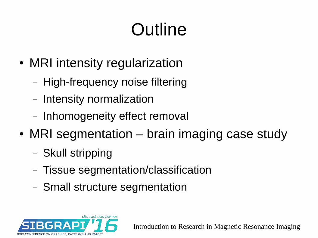
Outline
● MRI intensity regularization– High-frequency noise filtering
– Intensity normalization
– Inhomogeneity effect removal
● MRI segmentation – brain imaging case study– Skull stripping
– Tissue segmentation/classification
– Small structure segmentation
Introduction to Research in Magnetic Resonance Imaging
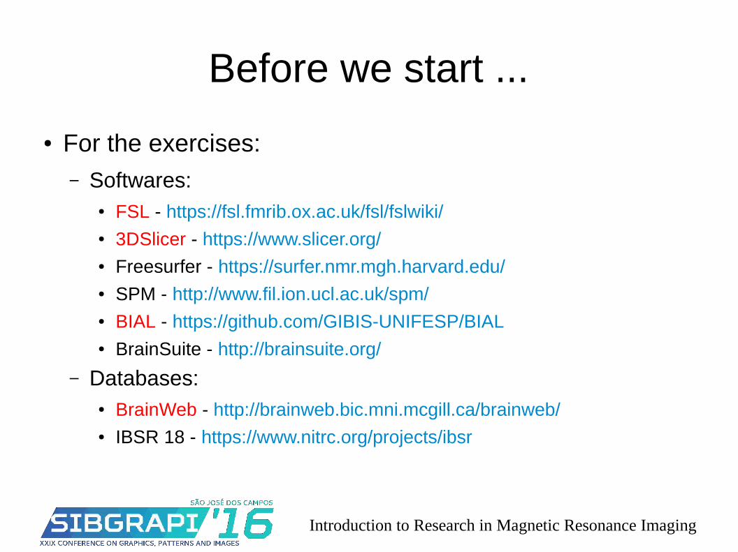
Before we start ...
● For the exercises:– Softwares:
● FSL - https://fsl.fmrib.ox.ac.uk/fsl/fslwiki/● 3DSlicer - https://www.slicer.org/● Freesurfer - https://surfer.nmr.mgh.harvard.edu/● SPM - http://www.fil.ion.ucl.ac.uk/spm/● BIAL - https://github.com/GIBIS-UNIFESP/BIAL ● BrainSuite - http://brainsuite.org/
– Databases:● BrainWeb - http://brainweb.bic.mni.mcgill.ca/brainweb/● IBSR 18 - https://www.nitrc.org/projects/ibsr
Introduction to Research in Magnetic Resonance Imaging
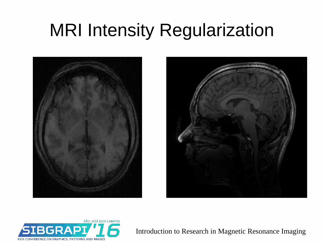
MRI Intensity Regularization
Introduction to Research in Magnetic Resonance Imaging
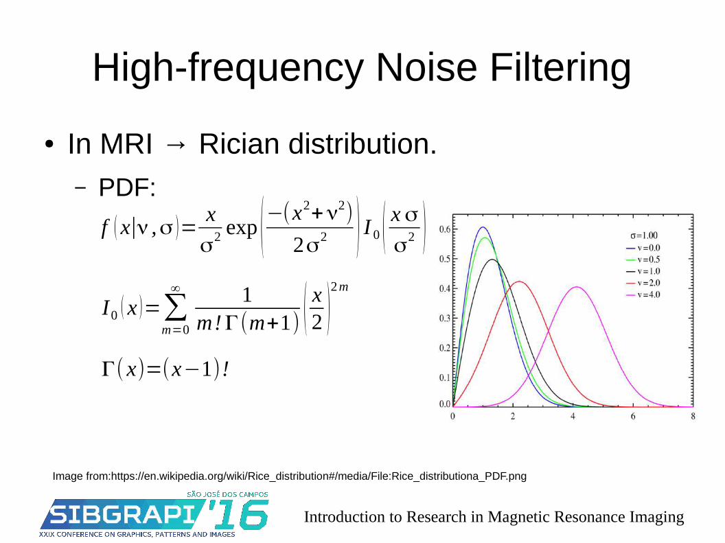
High-frequency Noise Filtering
● In MRI → Rician distribution.– PDF:
f ( x∣ν ,σ )=x
σ2 exp (−(x
2+ν2)
2σ2 ) I 0 ( x σσ2 )
I0 ( x )=∑m=0
∞ 1m!Γ(m+1) ( x2 )
2m
Γ( x)=(x−1)!
Image from:https://en.wikipedia.org/wiki/Rice_distribution#/media/File:Rice_distributiona_PDF.png
Introduction to Research in Magnetic Resonance Imaging
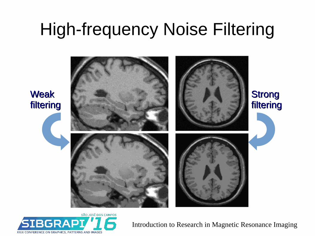
High-frequency Noise Filtering
WeakWeakfilteringfiltering
StrongStrongfilteringfiltering
Introduction to Research in Magnetic Resonance Imaging
High-frequency Noise Filtering
● 1st generation of filters: isotropics– e.g. Mean, median, gaussian
● 2nd generation of filters: local anisotropics– e.g. diffusion, bilateral [Smith 1997]
● 3rd generation of filters: non-local anisotropics– e.g. non-local means [Tristan-Vega 2012], BM3D,
PLOW
Introduction to Research in Magnetic Resonance Imaging
High-frequency Noise Filtering
● Isotropic filters:– Same operation over all pixels.
– Simplest → convolution.
– Fastest → O(n*a)
– Worst → borders also blurred.
Introduction to Research in Magnetic Resonance Imaging
High-frequency Noise Filtering
● Local anisotropic filters:– Adaptive filter, depending on pixel adjacency
contents.
– Relatively simple, mostly iterative process.
– Reasonably fast → O(n*a*i)
– Much better results – stronger edges preserved.
Introduction to Research in Magnetic Resonance Imaging
High-frequency Noise Filtering
● Non-local anisotropic filters:– Tries to get more information from adjacencies with similar
intensities or patterns of the filtered pixel.
– Very complex → requires clustering pixel patches.
– Very slow → O(nα*a*i).
– Best results → Estimates noise and removes it.
● Newest: http://www.nitrc.org/snapshots.php?group_id=518– [Tristan-Vega 2012]
– Compile with itk and add as module of 3DSlicer.
Introduction to Research in Magnetic Resonance Imaging
High-frequency Noise Filtering
● Exercise:– Open 3D slicer
● Run gradient anisotropic filtering over t1_pn5_rf40.
– Open FSL● Run Susan filtering over t1_pn5_rf40.
– Compare results and execution time.
Introduction to Research in Magnetic Resonance Imaging
High-frequency Noise Filtering
● Evaluation– PSNR, MSE → global.
– SSIM and variations such as MSSIM. [Wang 2004]→ structural.
● Today's use...– MRI is becoming almost noise free.
● 7 Tesla images are nice and clear … in some ways!
– Even supervised training with patches from multiple images was tested
● In medical images may generate incorrect results.
Introduction to Research in Magnetic Resonance Imaging
Intensity Normalization
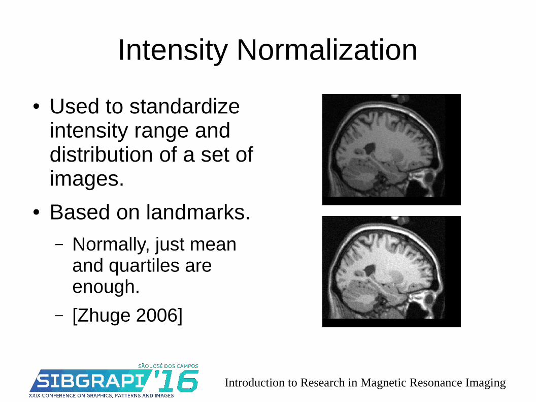
● Used to standardize intensity range and distribution of a set of images.
● Based on landmarks.– Normally, just mean
and quartiles are enough.
– [Zhuge 2006]
Introduction to Research in Magnetic Resonance Imaging
Intensity Normalization
● Two steps method– 1st – training: find landmarks in the histogram of
input image.
– 2nd – transformation: find landmarks in target images and map them to the ones of the training image.
Introduction to Research in Magnetic Resonance Imaging
Intensity Normalization
● Consequences:– Improves inhomogeneity correction.
– May improve segmentation process based on expected intensity ranges.
Introduction to Research in Magnetic Resonance Imaging
Intensity Inhomogeneity Correction
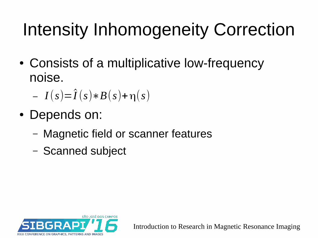
● Consists of a multiplicative low-frequency noise.–
● Depends on:– Magnetic field or scanner features
– Scanned subject
I (s)= I (s)∗B(s)+η(s)
Introduction to Research in Magnetic Resonance Imaging
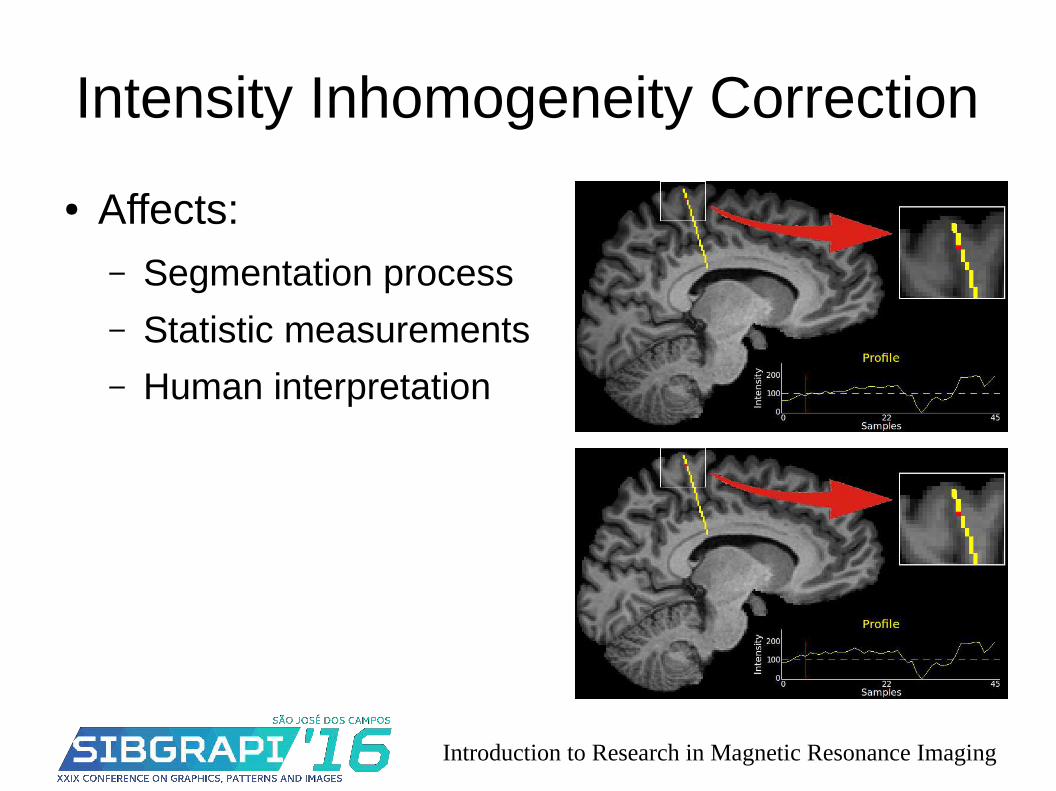
Intensity Inhomogeneity Correction
● Affects:– Segmentation process
– Statistic measurements
– Human interpretation
Introduction to Research in Magnetic Resonance Imaging
Intensity Inhomogeneity Correction
● General methods:– N3 [Sled 1998], N4 [Tustison 2010]
● Used over any kind of images.
● Brain specific methods:– BFC, FAST (also segments tissues)
● Used over skull stripped brain images.
Introduction to Research in Magnetic Resonance Imaging
Intensity Inhomogeneity Correction
● Exercise– Open 3D slicer
● Run N4itk inhomogeneity correction over t1_pn5_rf40.● Run N4itk inhomogeneity correction over t1_pn5_rf40
denoised.● Run gradient anisotropic filtering over t1_pn5_rf40
unbiased.
– Compare results.
Introduction to Research in Magnetic Resonance Imaging
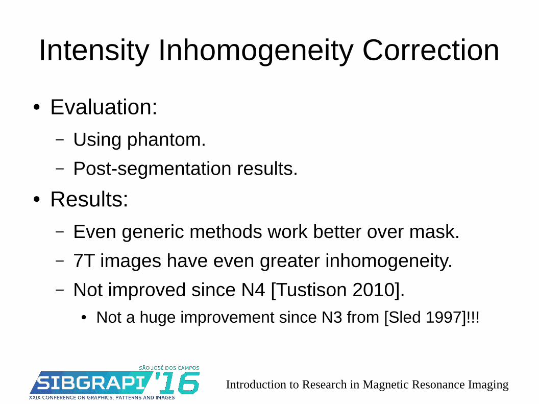
Intensity Inhomogeneity Correction
● Evaluation:– Using phantom.
– Post-segmentation results.
● Results:– Even generic methods work better over mask.
– 7T images have even greater inhomogeneity.
– Not improved since N4 [Tustison 2010]. ● Not a huge improvement since N3 from [Sled 1997]!!!
Introduction to Research in Magnetic Resonance Imaging
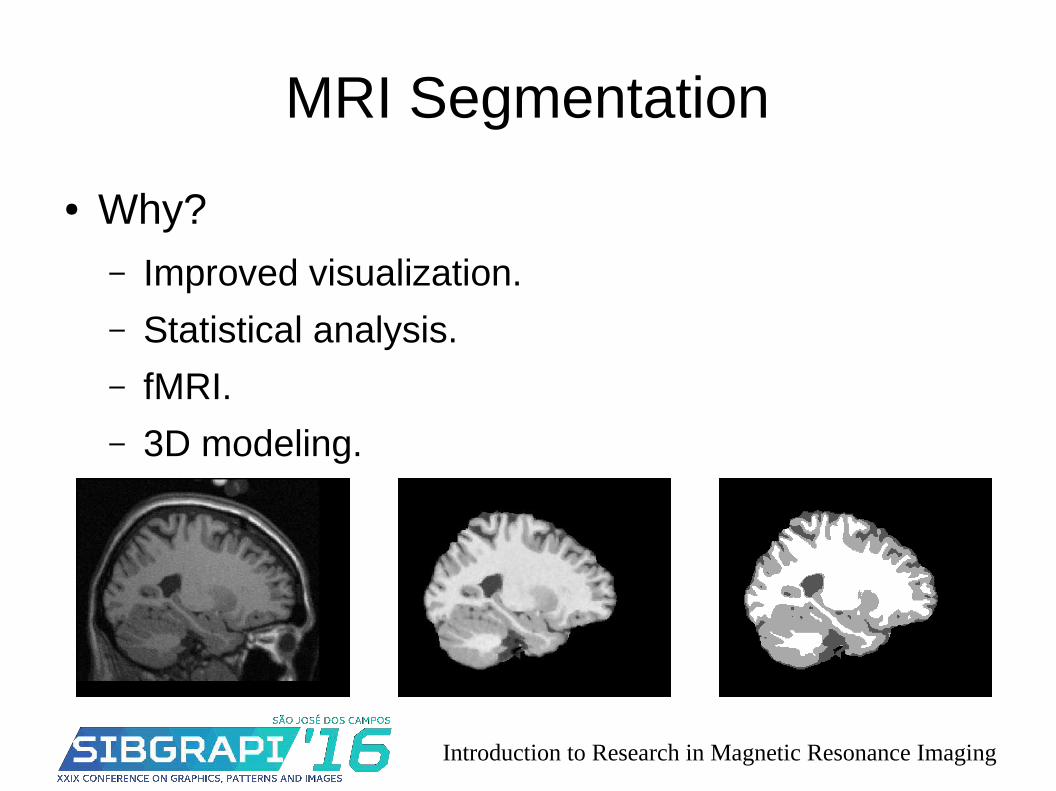
MRI Segmentation
● Why?– Improved visualization.
– Statistical analysis.
– fMRI.
– 3D modeling.
Introduction to Research in Magnetic Resonance Imaging
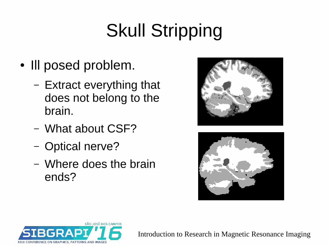
Skull Stripping
● Ill posed problem.– Extract everything that
does not belong to the brain.
– What about CSF?
– Optical nerve?
– Where does the brain ends?
Introduction to Research in Magnetic Resonance Imaging
Skull Stripping
● Methods:– Surface fitting:
● BET from FSL [Smith 2002].● BSE from BrainSuite.
– Region growing:● Hibrid watershed from Freesurfer. [Ségonne 2004]
– Mixed histogram matching:● SPM (also segments tissues)
Introduction to Research in Magnetic Resonance Imaging
Skull Stripping
● Exercise– Open FSL
● Run bet over t1_pn5_rf40.● Run bet over t1_pn5_rf40 denoised and unbiased.● Run bet with COG correction over t1_pn5_rf40 denoised
and unbiased.
– Compare results● Inhomogeneity correction effects [Miranda 2013]
Introduction to Research in Magnetic Resonance Imaging
Skull Stripping
● Evaluation:– Compare to manual segmentation. [Fennema‐
Notestine 2006]● Still, depends on human perception or goal application.
● Open questions:– No method generates perfect segmentation.
– Depends on inhomogeneity correction for high magnetic field MRI [Cappabianco 2012].
– Harder for pathological cases.
Introduction to Research in Magnetic Resonance Imaging
Tissue Segmentation
● Definition:– Label pixels into GM, WM, and CSF.
● Goal:– Allow quantization, analysis, fMRI studies.
● Issues:– What about partial volume pixels?
Introduction to Research in Magnetic Resonance Imaging
Tissue Segmentation
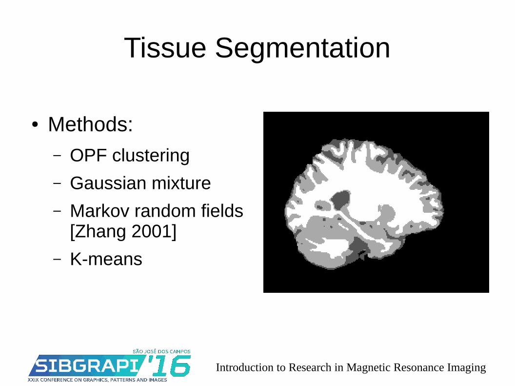
● Methods:– OPF clustering
– Gaussian mixture
– Markov random fields [Zhang 2001]
– K-means
Introduction to Research in Magnetic Resonance Imaging
Tissue Segmentation
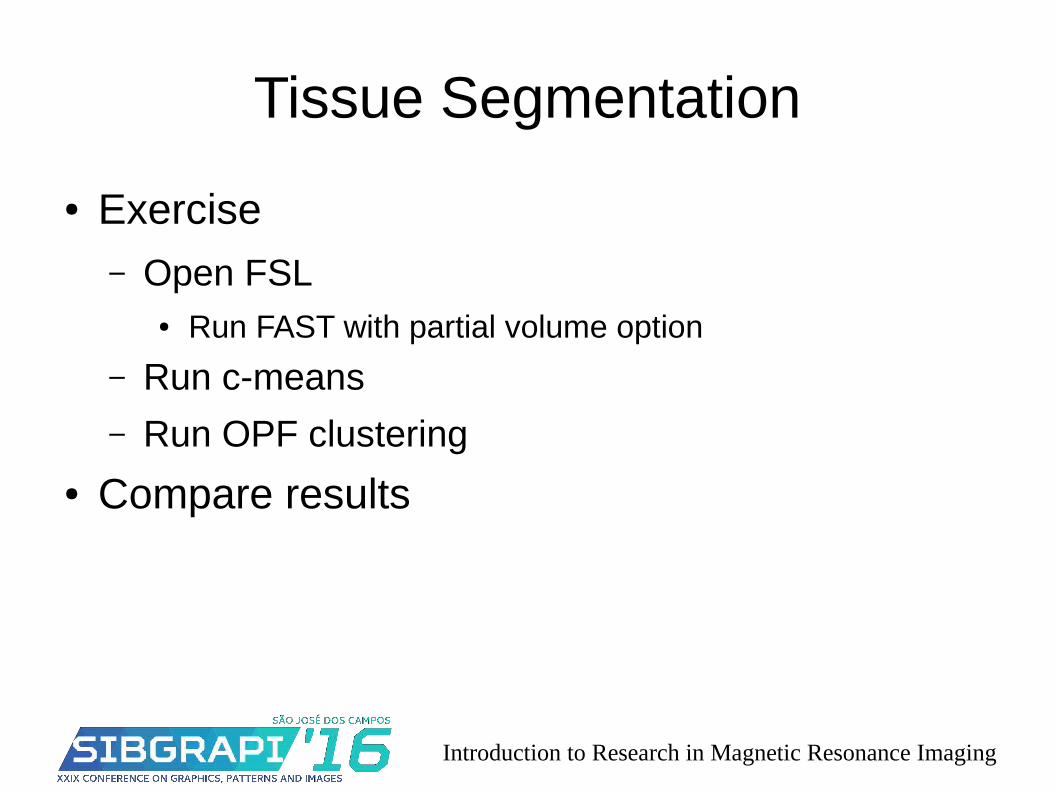
● Exercise– Open FSL
● Run FAST with partial volume option
– Run c-means
– Run OPF clustering
● Compare results
Introduction to Research in Magnetic Resonance Imaging
Tissue Segmentation
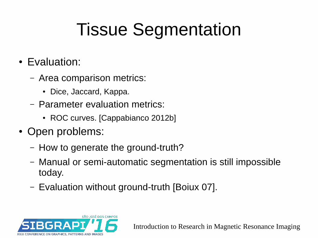
● Evaluation:– Area comparison metrics:
● Dice, Jaccard, Kappa.
– Parameter evaluation metrics:● ROC curves. [Cappabianco 2012b]
● Open problems:– How to generate the ground-truth?
– Manual or semi-automatic segmentation is still impossible today.
– Evaluation without ground-truth [Boiux 07].
Introduction to Research in Magnetic Resonance Imaging
Small Structure Segmentation
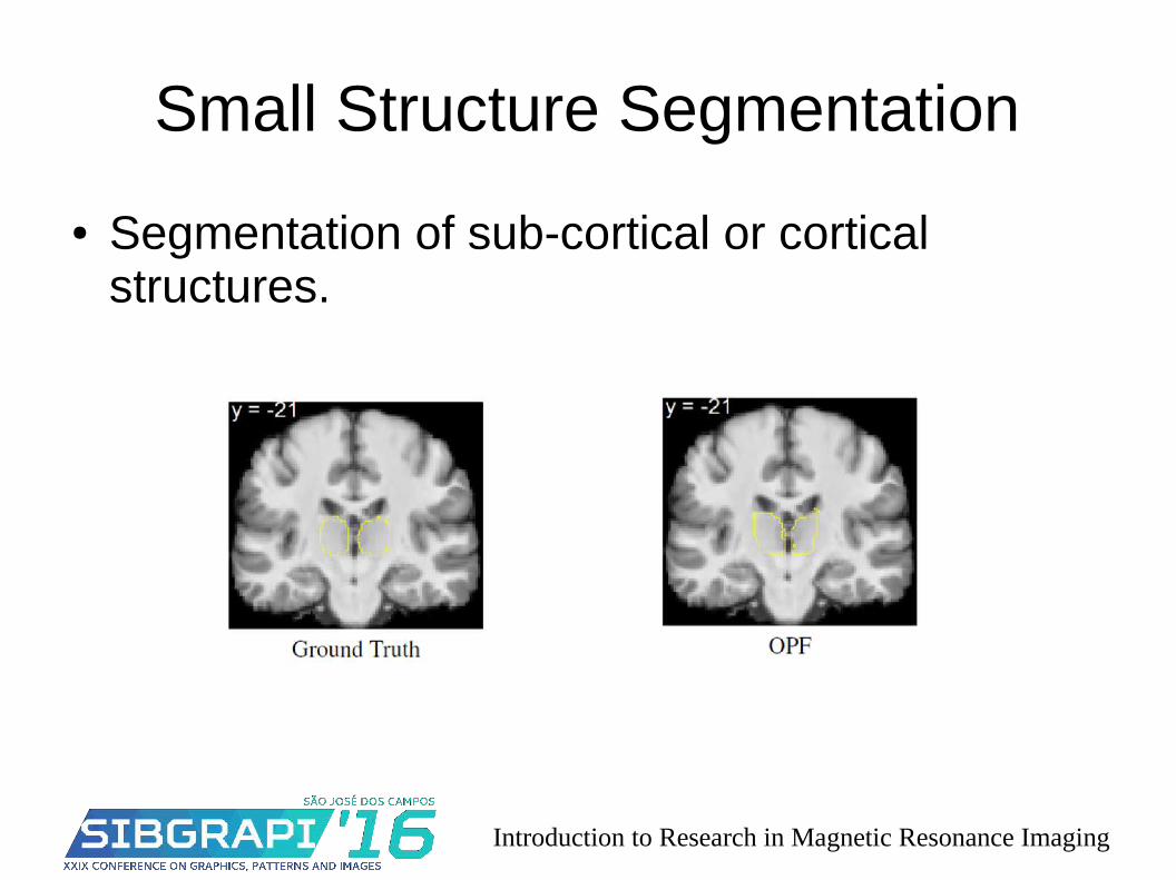
● Segmentation of sub-cortical or cortical structures.
Introduction to Research in Magnetic Resonance Imaging
Small Structure Segmentation
● User iteration types– Automatic
– Manual
– Semi-automatic
● Implementation types– Region growing
– Edge delineation
Introduction to Research in Magnetic Resonance Imaging
Other operations
● Pose estimation.● Brain alignment.● Surface extraction.● Hemisphere symmetry analysis● Registration● …
Introduction to Research in Magnetic Resonance Imaging
References
[Smith 1997] Smith, Stephen M., and J. Michael Brady. "SUSAN—a new approach to low level image processing." International journal of computer vision 23.1 (1997): 45-78.
[Black 1998] Black, Michael J., et al. "Robust anisotropic diffusion." IEEE Transactions on image processing 7.3 (1998): 421-432.
[Sled 1998] Sled, John G., Alex P. Zijdenbos, and Alan C. Evans. "A nonparametric method for automatic correction of intensity nonuniformity in MRI data." IEEE transactions on medical imaging 17.1 (1998): 87-97.
[Zhang 2001] Zhang, Yongyue, Michael Brady, and Stephen Smith. "Segmentation of brain MR images through a hidden Markov random field model and the expectation-maximization algorithm." IEEE transactions on medical imaging 20.1 (2001): 45-57.
[Smith 2002] Smith, Stephen M. "Fast robust automated brain extraction." Human brain mapping 17.3 (2002): 143-155.
[Ségonne 2004] Ségonne, Florent, et al. "A hybrid approach to the skull stripping problem in MRI." Neuroimage 22.3 (2004): 1060-1075.
[Wang 2004] Wang, Zhou, et al. "Image quality assessment: from error visibility to structural similarity." IEEE transactions on image processing 13.4 (2004): 600-612.
[Fennema‐Notestine 2006] Fennema‐Notestine, Christine, et al. "Quantitative evaluation of automated skull‐stripping methods applied to contemporary and legacy images: Effects of diagnosis, bias correction, and slice location." Human brain mapping 27.2 (2006): 99-113.
Introduction to Research in Magnetic Resonance Imaging
References
[Zhuge 2006] Zhuge, Ying, et al. "An intensity standardization-based method for image inhomogeneity correction in MRI." Medical Imaging. International Society for Optics and Photonics, 2006.
[Bouix 2007] Bouix, Sylvain, et al. "On evaluating brain tissue classifiers without a ground truth." Neuroimage 36.4 (2007): 1207-1224.
[Tustison 2010] Tustison, Nicholas J., et al. "N4ITK: improved N3 bias correction." IEEE transactions on medical imaging 29.6 (2010): 1310-1320.
[Cappabianco 2012] Cappabianco, Fábio AM, et al. "Unraveling the compromise between skull stripping and inhomogeneity correction in 3T MR images." 2012 25th SIBGRAPI Conference on Graphics, Patterns and Images. IEEE, 2012.
[Cappabianco 2012b] Cappabianco, Fábio AM, et al. "Brain tissue MR-image segmentation via optimum-path forest clustering." Computer Vision and Image Understanding 116.10 (2012): 1047-1059.
[Miranda 2013] Miranda, Paulo AV, Fábio AM Cappabianco, and Jaime S. Ide. "A case analysis of the impact of prior center of gravity estimation over skull-stripping algorithms in mr images." 2013 IEEE International Conference on Image Processing. IEEE, 2013.
[Tristán-Vega 2012] Tristán-Vega, Antonio, et al. "Efficient and robust nonlocal means denoising of MR data based on salient features matching." Computer methods and programs in biomedicine 105.2 (2012): 131-144.
Introduction to Research in Magnetic Resonance Imaging
Extras
Introduction to Research in Magnetic Resonance Imaging
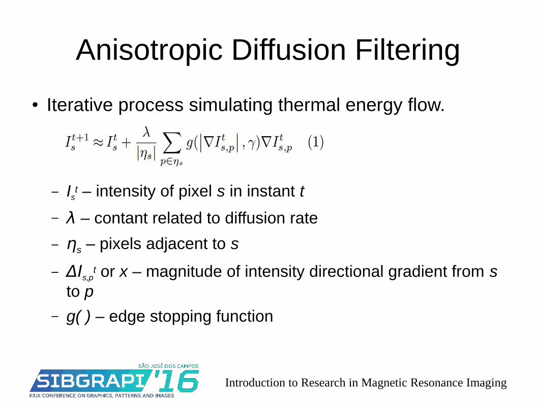
Anisotropic Diffusion Filtering
● Iterative process simulating thermal energy flow.
– Ist – intensity of pixel s in instant t
– λ – contant related to diffusion rate
– ηs – pixels adjacent to s
– ΔIs,pt or x – magnitude of intensity directional gradient from s
to p
– g( ) – edge stopping function
Introduction to Research in Magnetic Resonance Imaging
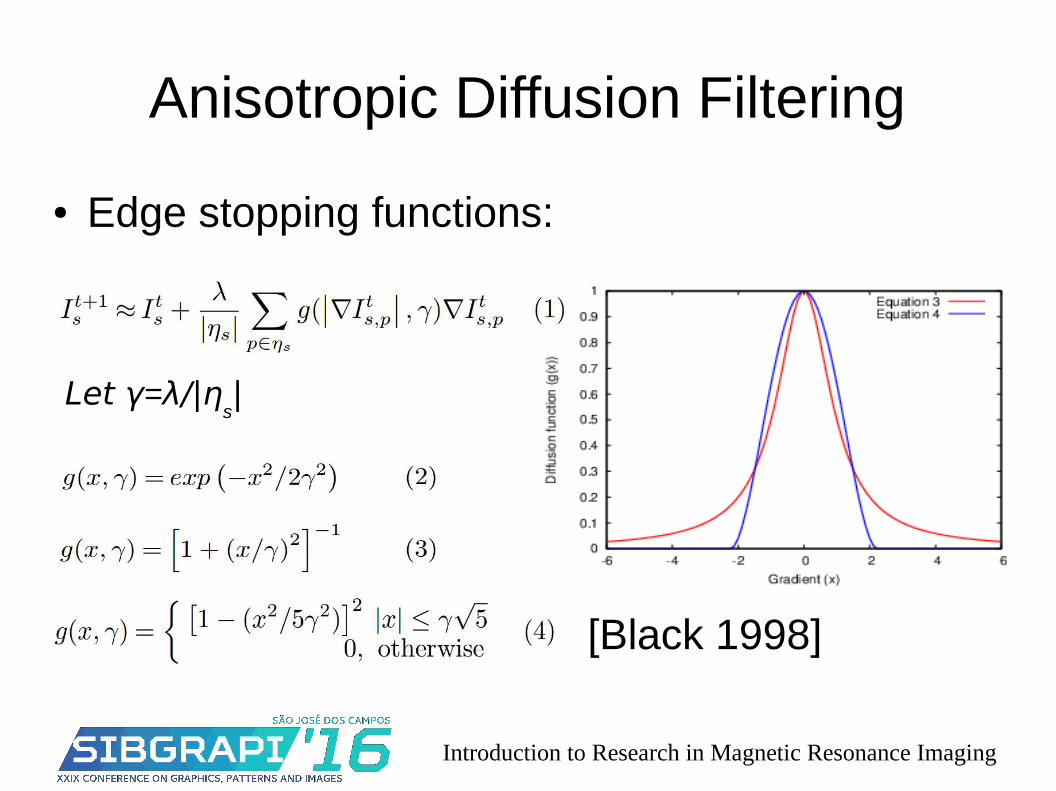
Anisotropic Diffusion Filtering
Let γ=λ/|ηs|
● Edge stopping functions:
[Black 1998]
Introduction to Research in Magnetic Resonance Imaging
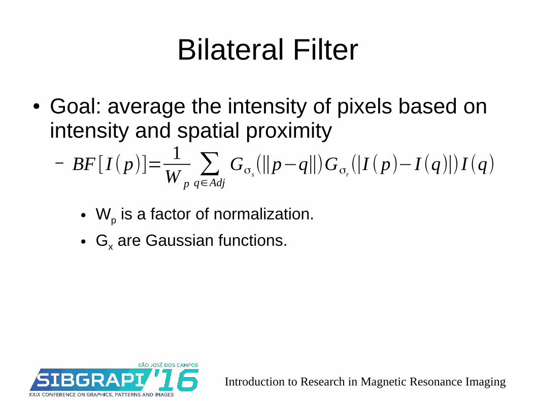
Bilateral Filter
● Goal: average the intensity of pixels based on intensity and spatial proximity–
● Wp is a factor of normalization.
● Gx are Gaussian functions.
BF [ I (p)]=1W p
∑q∈Adj
Gσs(‖p−q‖)Gσr
(|I (p)−I (q)|) I (q)
Introduction to Research in Magnetic Resonance Imaging
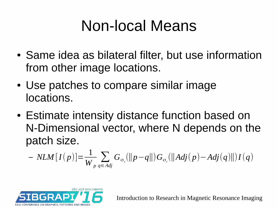
Non-local Means
● Same idea as bilateral filter, but use information from other image locations.
● Use patches to compare similar image locations.
● Estimate intensity distance function based on N-Dimensional vector, where N depends on the patch size.– NLM [ I ( p)]=
1W p
∑q∈ Adj
Gσ s(‖p−q‖)Gσ r
(‖Adj( p)−Adj(q)‖) I (q)
Introduction to Research in Magnetic Resonance Imaging
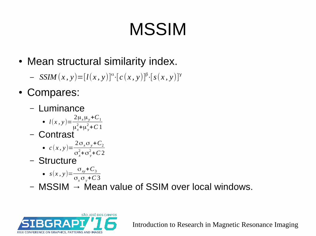
MSSIM
● Mean structural similarity index.–
● Compares:– Luminance
●
– Contrast●
– Structure●
– MSSIM → Mean value of SSIM over local windows.
l(x , y )=2μ xμ y+C1
μ x2+μ y
2+C 1
c (x , y )=2σ xσ y+C2
σ x2+σ y
2+C 2
s(x , y )=σ xy+C3
σxσ y+C 3
SSIM (x , y)=[l(x , y)]α⋅[c (x , y)]β⋅[s(x , y)]γ
Introduction to Research in Magnetic Resonance Imaging
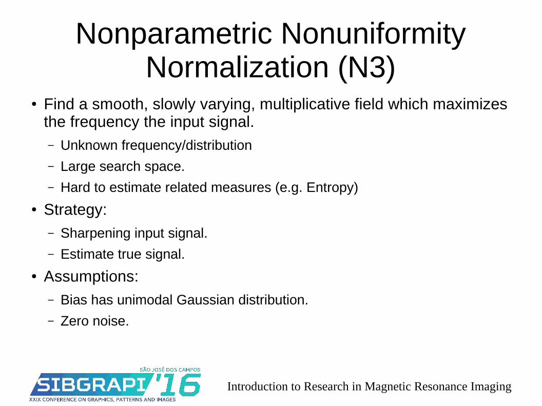
Nonparametric NonuniformityNormalization (N3)
● Find a smooth, slowly varying, multiplicative field which maximizes the frequency the input signal.– Unknown frequency/distribution
– Large search space.
– Hard to estimate related measures (e.g. Entropy)
● Strategy:– Sharpening input signal.
– Estimate true signal.
● Assumptions:– Bias has unimodal Gaussian distribution.
– Zero noise.
Introduction to Research in Magnetic Resonance Imaging
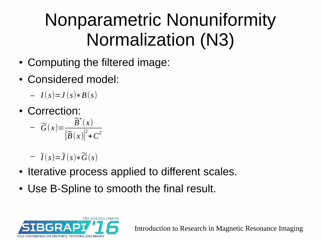
Nonparametric NonuniformityNormalization (N3)
● Computing the filtered image:● Considered model:
–
● Correction:–
–
● Iterative process applied to different scales.● Use B-Spline to smooth the final result.
I (s)=J (s)∗B (s)
~G (x)=~B*
(x)
|~B (x)|2+C2
~I (s)=~J (s)∗~G (s)
Introduction to Research in Magnetic Resonance Imaging
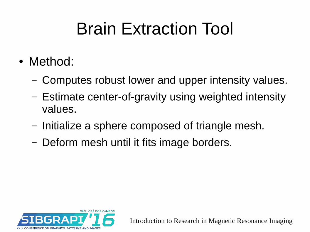
Brain Extraction Tool
● Method:– Computes robust lower and upper intensity values.
– Estimate center-of-gravity using weighted intensity values.
– Initialize a sphere composed of triangle mesh.
– Deform mesh until it fits image borders.
Introduction to Research in Magnetic Resonance Imaging
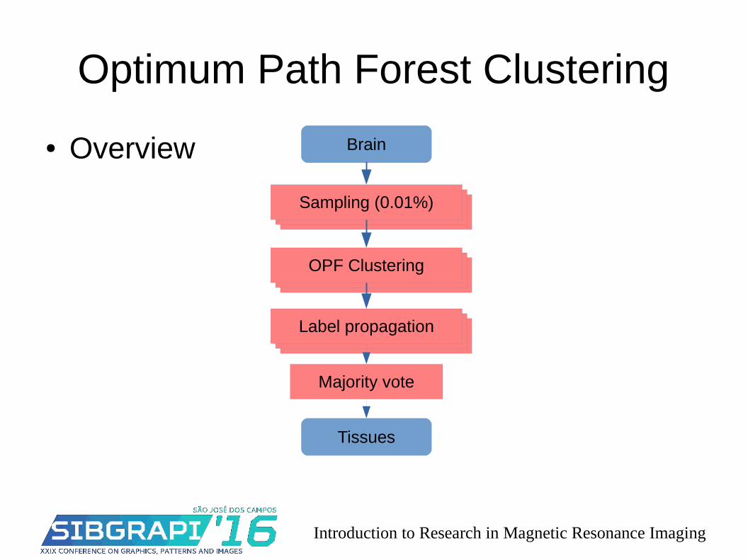
Optimum Path Forest Clustering
Brain
Tissues
Sampling (0.01%)
OPF Clustering
Label propagation
Majority vote
● Overview
Introduction to Research in Magnetic Resonance Imaging
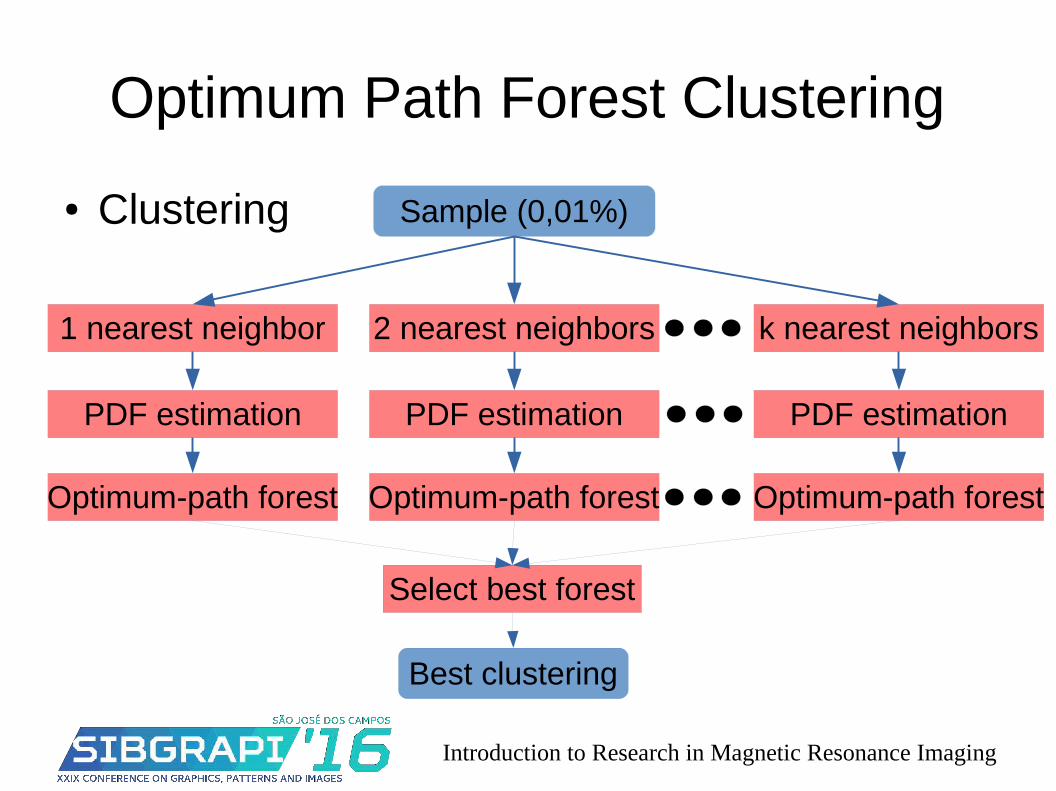
Optimum Path Forest Clustering
● Clustering Sample (0,01%)
Best clustering
1 nearest neighbor
PDF estimation
Optimum-path forest
2 nearest neighbors
PDF estimation
Optimum-path forest
k nearest neighbors
PDF estimation
Optimum-path forest
Select best forest
Introduction to Research in Magnetic Resonance Imaging
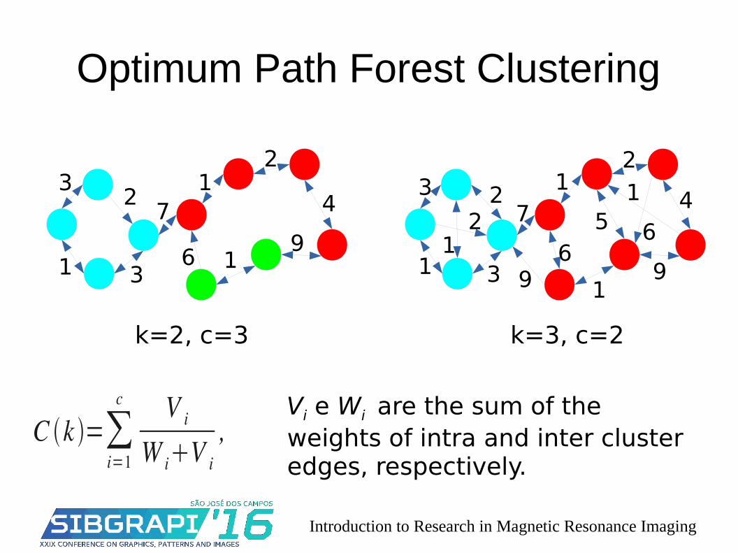
Optimum Path Forest Clustering
C k =∑i=1
c V i
W iV i
, Vi e Wi are the sum of the
weights of intra and inter cluster edges, respectively.
k=2, c=3 k=3, c=2
32
1 3
71
2
4
916
3
1
2
3
21
71
2
4
919
65
1
6
Introduction to Research in Magnetic Resonance Imaging
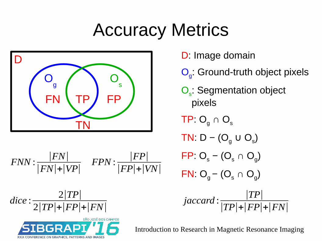
Accuracy MetricsD: Image domain
Og: Ground-truth object pixels
Os: Segmentation object pixels
TP: Og ∩ Os
TN: D − (Og O∪ s)
FP: Os − (Os ∩ Og)
FN: Og − (Os ∩ Og)
D
FN TP FP
Og
Os
TN
FPN :|FP|
|FP|+|VN|FNN :
|FN||FN|+|VP|
dice :2|TP|
2|TP|+|FP|+|FN|jaccard :
|TP||TP|+|FP|+|FN|

V. POSE AND SPATIAL STANDARDIZATION
Sibigrapi – São José dos Campos
2016
Claudio Shida
Email: [email protected]
A.Image interpolationB.Motion correctionC.Image registration
Summary
A. Image interpolation
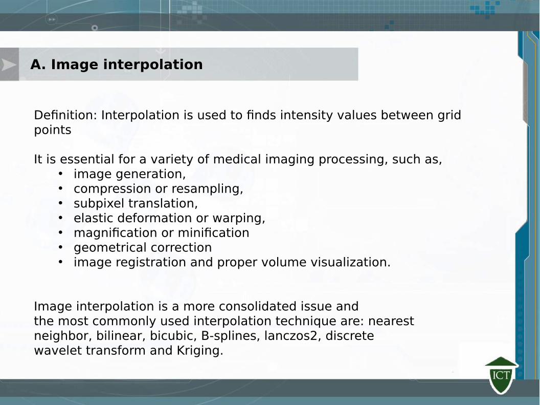
Definition: Interpolation is used to finds intensity values between grid points
It is essential for a variety of medical imaging processing, such as, • image generation, • compression or resampling, • subpixel translation, • elastic deformation or warping,• magnification or minification• geometrical correction• image registration and proper volume visualization.
Image interpolation is a more consolidated issue andthe most commonly used interpolation technique are: nearestneighbor, bilinear, bicubic, B-splines, lanczos2, discretewavelet transform and Kriging.
A. Image interpolation
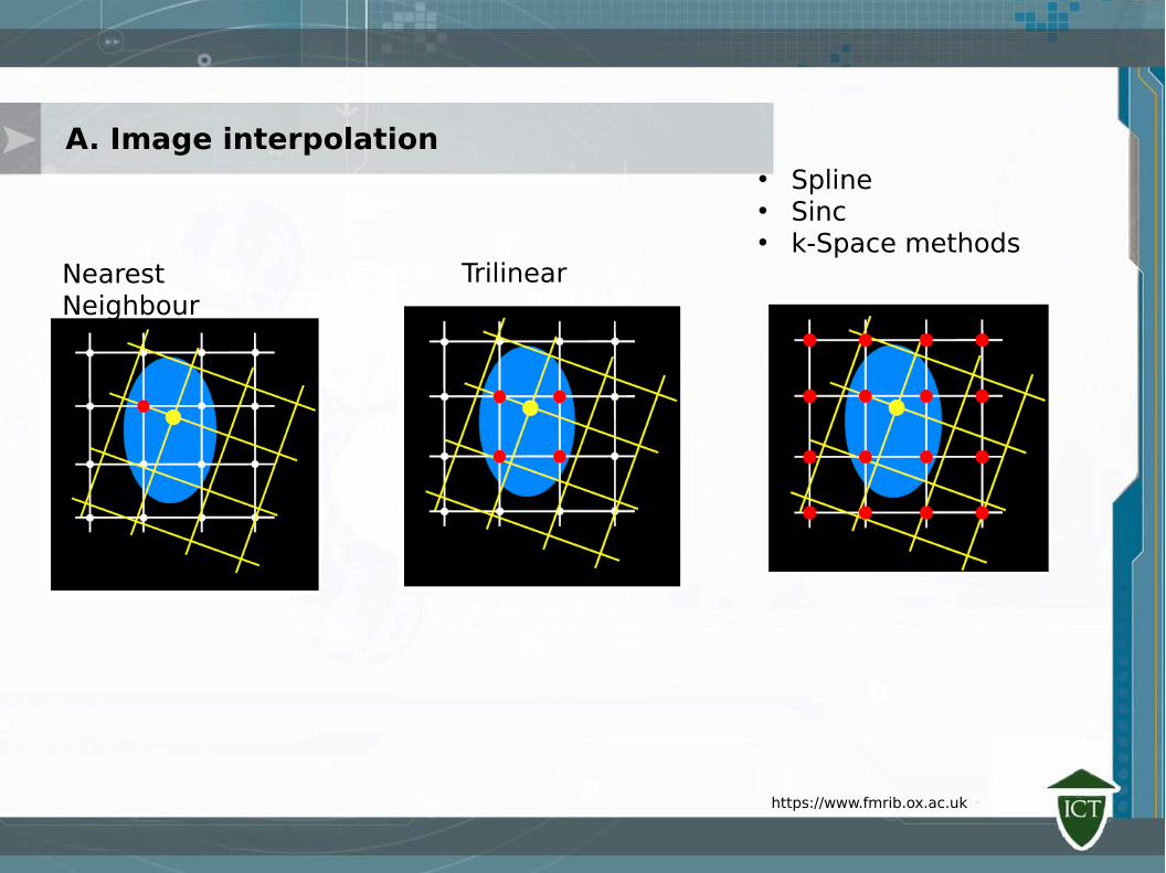
TrilinearNearest Neighbour
• Spline• Sinc• k-Space methods
https://www.fmrib.ox.ac.uk
A. Image interpolation - References
J. Ashburner and C. D. Good, “Spatial registration of images,” in Quantitative MRI of the Brain: Measuring Changes Caused by Disease, P. Tofts, Ed. John Wiley & Sons, 2003, ch. 15, pp. 503–532.
T. M. Lehmann, C. Gonner, and K. Spitzer, “Survey: Interpolation methods in medical image processing,” IEEE TRANSACTIONS ON MEDICAL IMAGING, vol. 18, no. 11, pp. 1049–1075, 1999.
E. H. W. Meijering, “Spline interpolation in medical imaging: comparison with other convolution-based approaches,” Proceedings of EUSIPCO 2000, M. Gabbouj and P. Kuosmanen (eds.), vol. IV, pp. 1989–1996, 2000.
A. Amanatiadis and I. Andreadis, “A survey on evaluation methods for image interpolation,” Measurement Science and Technology, vol. 20, no. 10, p. 104015, 2009.
B. Motion correction
Patient may move the head during a run or between runs, resulting in wrong spatial location.
-impossible to avoid movements as small as a few millimeters. - It will dishevel or distort the image sequence.
The motion correction should be carried out co-registering each volume in the sequence run acquisition to a reference volume.
The reference volume may be: i) First volume in the sequence acquisition; ii) Middle volume in the sequence acquisition; or iii) Average of all the volumes in the sequence acquisition prior to motion correction.
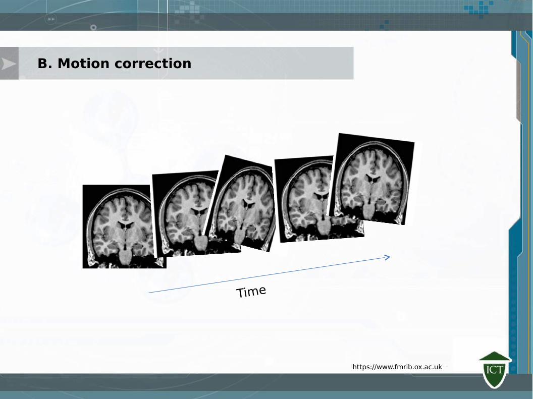
B. Motion correction
Time
https://www.fmrib.ox.ac.uk
Most commonly used interpolation technique are: • Earest neighbor, • bilinear, • Trilinear,• bicubic, • B-splines, • lanczos2, • discrete• wavelet transform and Kriging [89].
B. Motion correction
C. Image registration
• Image Registration is the process of estimating an optimal transformation between two images.
• Sometimes also known as “Spatial Normalization”
C. Image registration
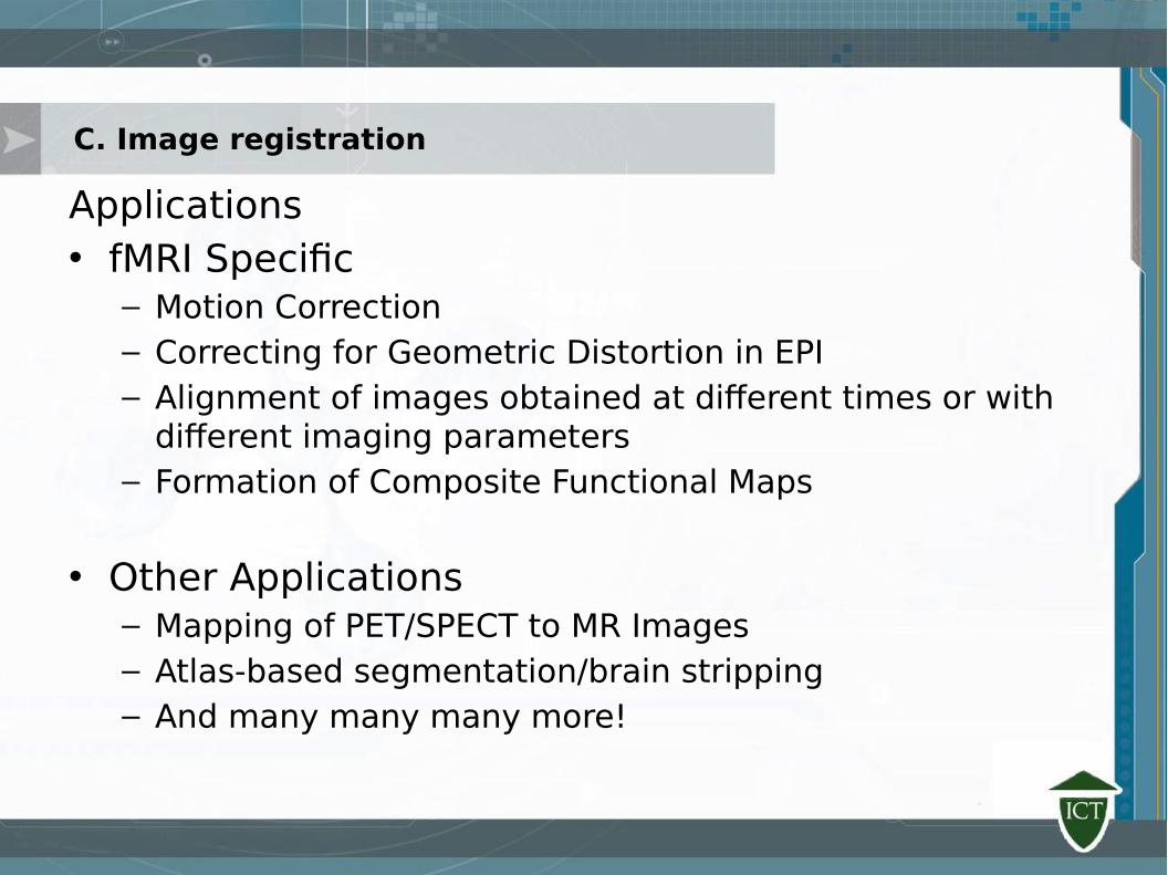
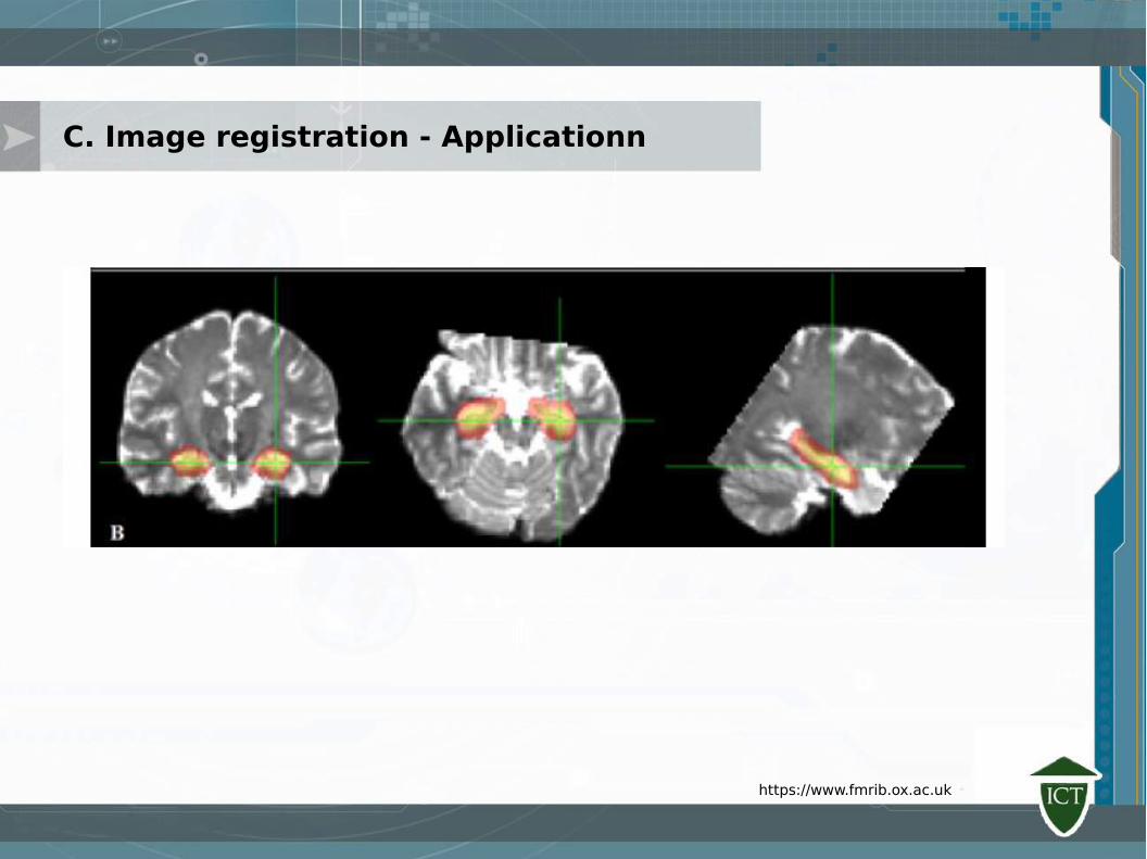
Applications• fMRI Specific
– Motion Correction– Correcting for Geometric Distortion in EPI– Alignment of images obtained at different times or with
different imaging parameters– Formation of Composite Functional Maps
• Other Applications– Mapping of PET/SPECT to MR Images– Atlas-based segmentation/brain stripping– And many many many more!
C. Image registration
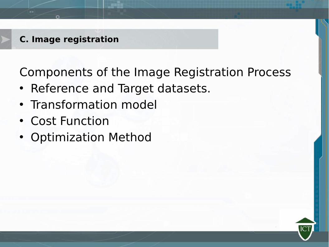
Components of the Image Registration Process• Reference and Target datasets.• Transformation model• Cost Function• Optimization Method
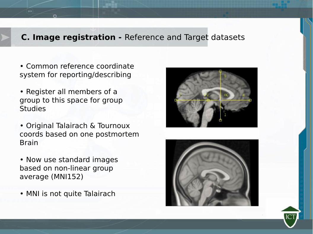
C. Image registration - Reference and Target datasets
• Common reference coordinatesystem for reporting/describing
• Register all members of agroup to this space for groupStudies
• Original Talairach & Tournouxcoords based on one postmortemBrain
• Now use standard imagesbased on non-linear groupaverage (MNI152)
• MNI is not quite Talairach
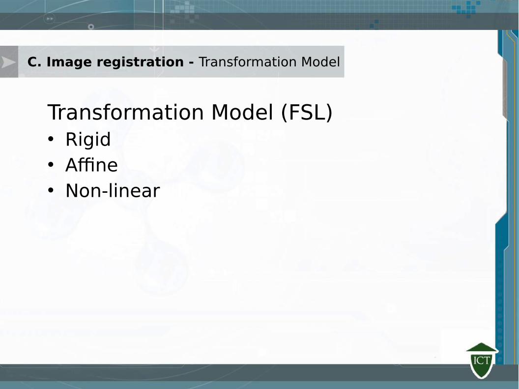
C. Image registration - Transformation Model
Transformation Model (FSL)• Rigid • Affine• Non-linear
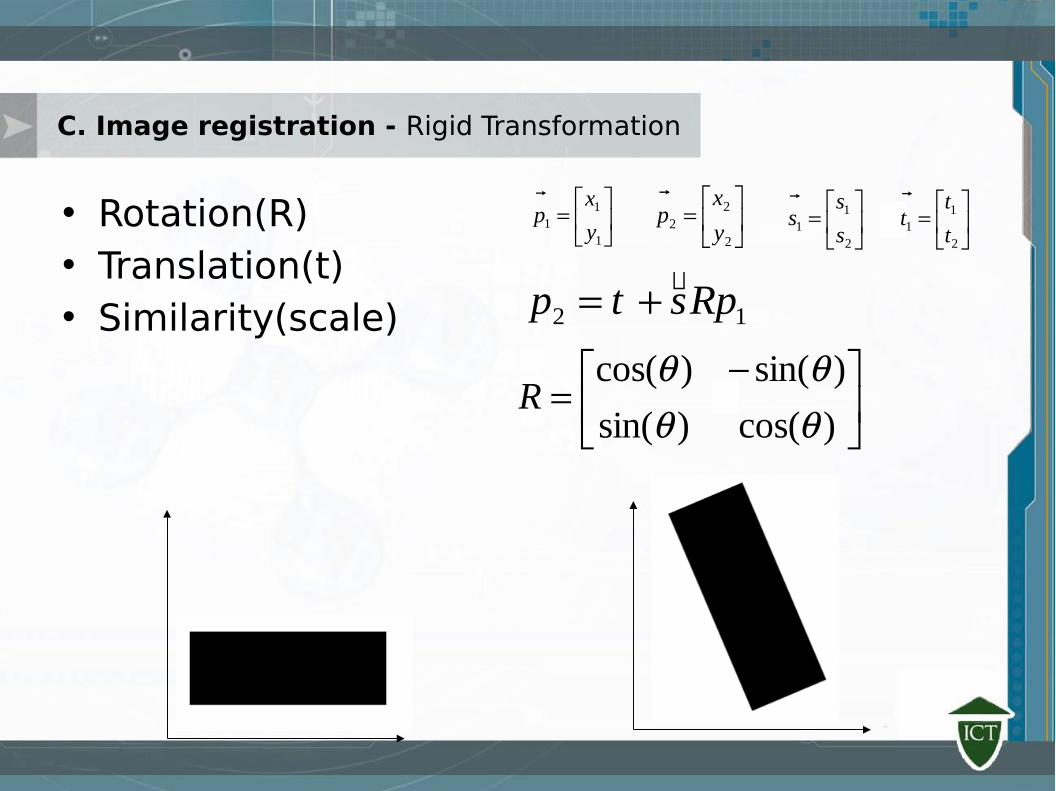
C. Image registration - Rigid Transformation
• Rotation(R)• Translation(t)• Similarity(scale)
2
22 y
xp
1
11 y
xp
12 pRstp
)cos()sin(
)sin()cos(
R
2
11 s
ss
2
11 t
tt
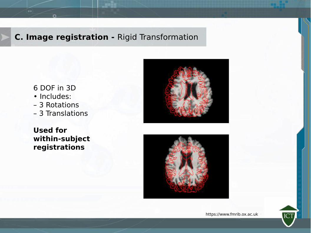
6 DOF in 3D• Includes:– 3 Rotations– 3 Translations
Used forwithin-subjectregistrations
C. Image registration - Rigid Transformation
https://www.fmrib.ox.ac.uk

C. Image registration - Affine Transformation
• Rotation• Translation• Scale• Shear
No more preservation of lengths and angles
Parallel lines are preserved
1
1
2221
1211
23
13
2
2
y
x
aa
aa
a
a
y
x
www.comp.nus.edu.sg/~cs4243/lecture/register
C. Image registration - Affine Transformation
12 DOF in 3D• Linear Transf.• Includes:– 3 Rotations– 3 Translations– 3 Scalings– 3 Skews/Shears
Used for eddy current correctionand initialising non-linear registration
https://www.fmrib.ox.ac.uk
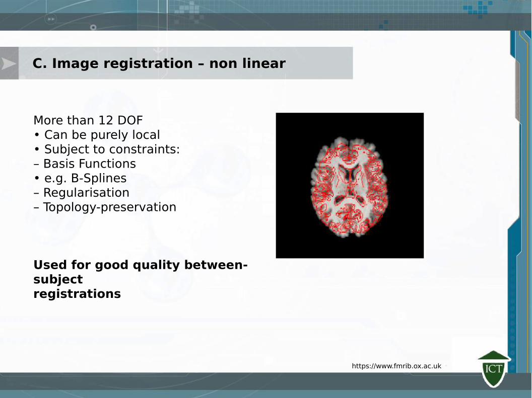
C. Image registration – non linear
More than 12 DOF• Can be purely local• Subject to constraints:– Basis Functions• e.g. B-Splines– Regularisation– Topology-preservation
Used for good quality between-subjectregistrations
https://www.fmrib.ox.ac.uk
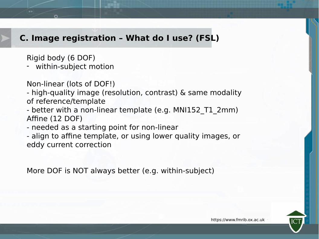
Rigid body (6 DOF)- within-subject motion
Non-linear (lots of DOF!)- high-quality image (resolution, contrast) & same modalityof reference/template- better with a non-linear template (e.g. MNI152_T1_2mm)Affine (12 DOF)- needed as a starting point for non-linear- align to affine template, or using lower quality images, oreddy current correction
More DOF is NOT always better (e.g. within-subject)
C. Image registration – What do I use? (FSL)
https://www.fmrib.ox.ac.uk
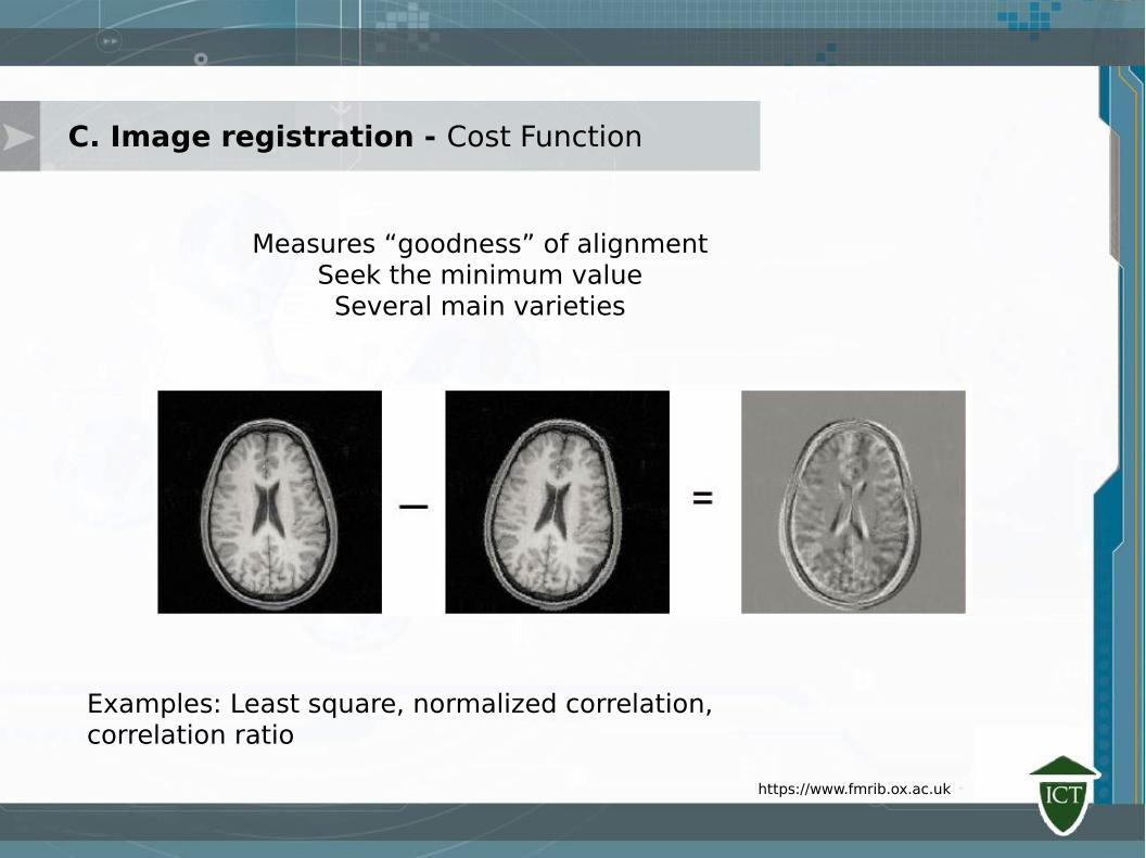
C. Image registration - Cost Function
Measures “goodness” of alignmentSeek the minimum value
Several main varieties
Examples: Least square, normalized correlation, correlation ratio
https://www.fmrib.ox.ac.uk
C. Image registration - Applicationn
https://www.fmrib.ox.ac.uk
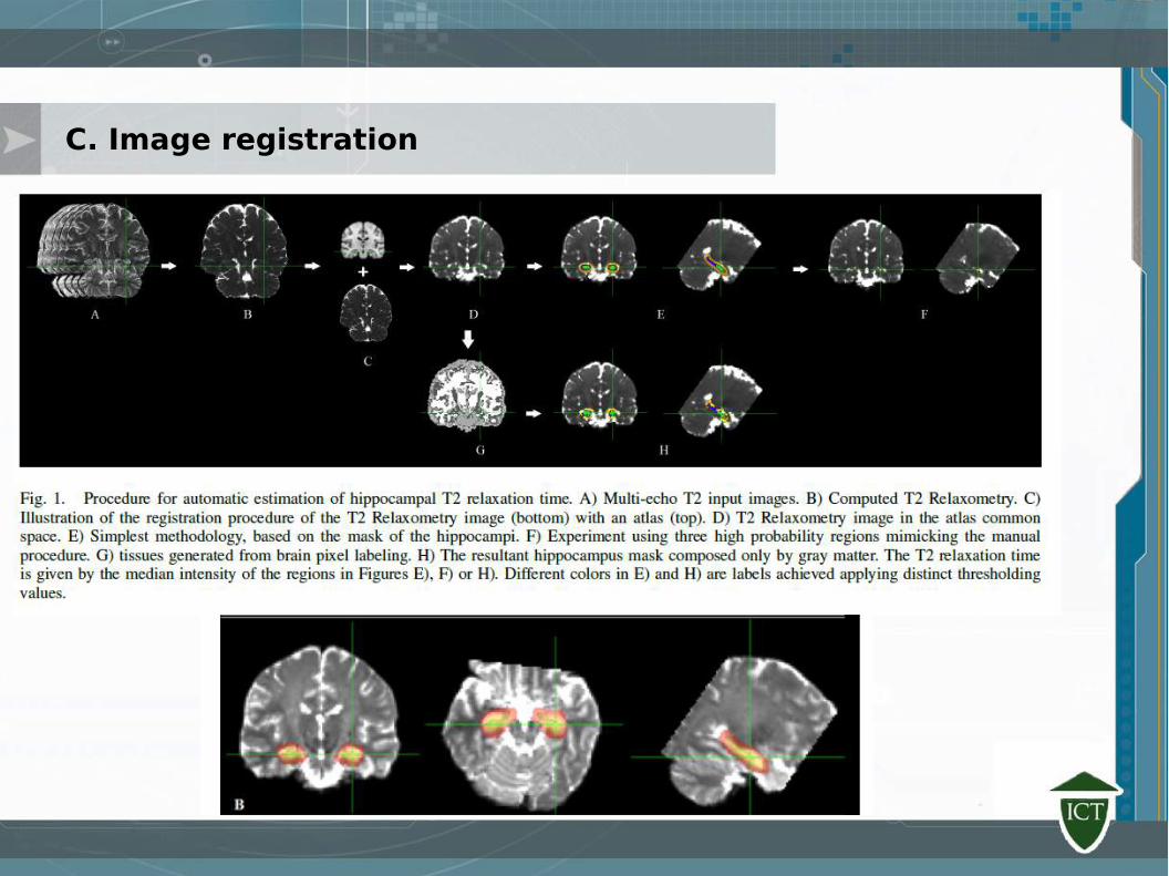
C. Image registration
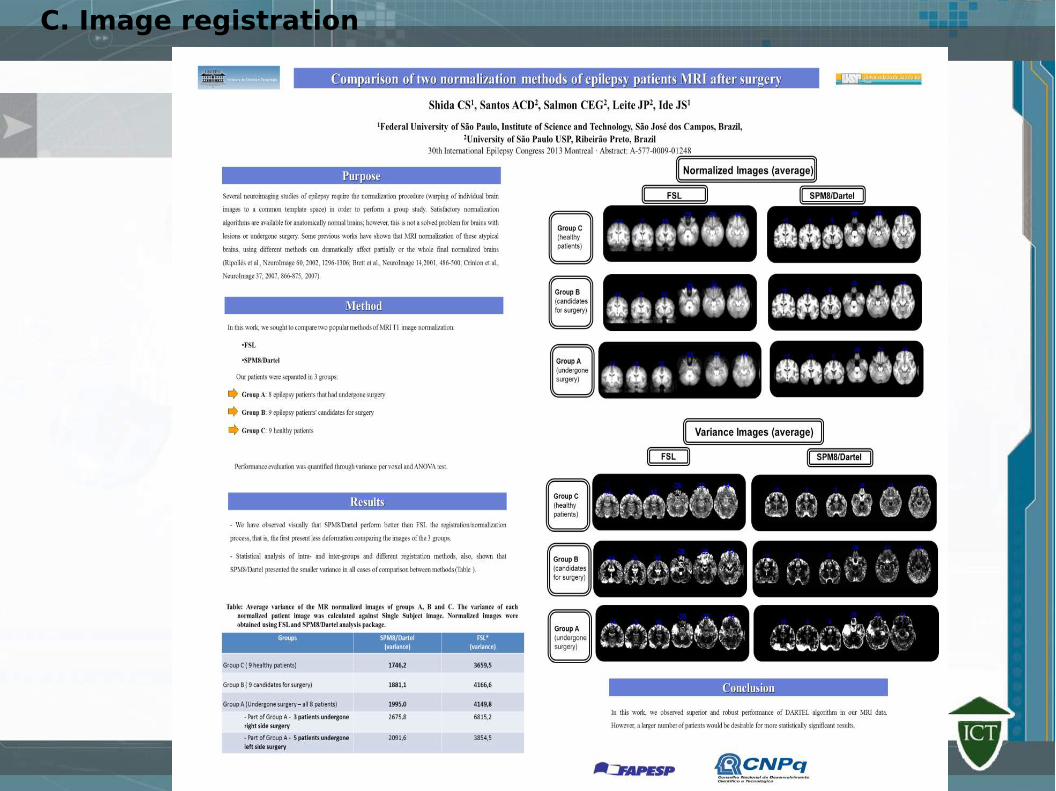
C. Image registration
C. Image registration - References
- P. A. Miranda, F. A. Cappabianco, and J. S. Ide, “A case analysis of the impact of prior center of gravity estimation over skull-stripping algorithms in mr images,” in 2013 IEEE International Conference on Image Processing. IEEE, 2013, pp. 675–679.- M. Brett, I. S. Johnsrude, and A. M. Owen, “The problem of functional localization in the human brain,” Nature reviews neuroscience, vol. 3, no. 3, pp. 243–249, 2002.- A. Klein, J. Anderssonb, B. A. Ardekani, J. Ashburner, B. Avants, M.-C. Chiang, G. E. Christensen, D. L. Collins, J. Gee, P. Hellier, J. H. Song, M. Jenkinson, C. Lepage, D. Rueckert, P. Thompson, T. Vercauteren, R. P. Woods, J. J. Mann, and R. V. Parsey, “Evaluation of 14 nonlinear deformation algorithms applied to human brain mri registration,” NeuroImage, vol. 46, no. 3, p. 786802, 2009.- M. Jenkinson, C. F. Beckmann, T. E. Behrens, M. W. Woolrich, and S. Smith, “Fsl,” NeuroImage, vol. 62, no. 2, pp. 782–790, 2001. - J. L. Andersson, M. Jenkinson, S. Smith et al., “Non-linear registration, aka spatial normalisation fmrib technical report tr07ja2,” FMRIB Analysis Group of the University of Oxford, vol. 2, 2007.- B. B. Avants, N. Tustison, and G. Song, “Advanced normalization tools (ants),” Insight J, vol. 2, pp. 1–35, 2009.- N. J. Tustison, P. A. Cook, A. Klein, G. Song, S. R. Das, J. T. Duda, B. M. Kandel, N. van Strien, J. R. Stone, J. C. Gee et al., “Large-scale evaluation of ants and freesurfer cortical thickness measurements,”Neuroimage, vol. 99, pp. 166–179, 2014.- S. Klein, M. Staring, K. Murphy, M. A. Viergever, and J. P. Pluim, “Elastix: a toolbox for intensity-based medical image registration,” IEEE transactions on medical imaging, vol. 29, no. 1, pp. 196–205,2010.- J. West and et al., “Comparison and evaluation of retrospective intermodality brain image registration techniques,” Journal of Computer Assisted Tomography, vol. 21, no. 4, pp. 554–566, 1997.- M. Jenkinson and S. Smith, “A global optimisation method for robust affine registration of brain images,” Medical Image Analysis, vol. 5, pp. 143–156, 2001.- M. Jenkinson, P. Bannister, M. Brady, and S. Smith, “Improved optimization for the robust and accurate linear registration and motion correction of brain images,” Neuroimage, vol. 17, no. 2, pp. 825–841, 2002.

Principles of fMRIGilson Vieira and Kelly Cotosck
Ph. D. in Bioinformaticsand Ph. D. student in Neuroimaging at University of São Paulo
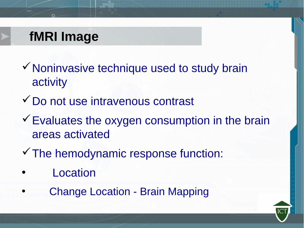
fMRI Image
Noninvasive technique used to study brain activity
Do not use intravenous contrast
Evaluates the oxygen consumption in the brain areas activated
The hemodynamic response function:
• Location
• Change Location - Brain Mapping
https://br.pinterest.com/pin/465418942711773729/
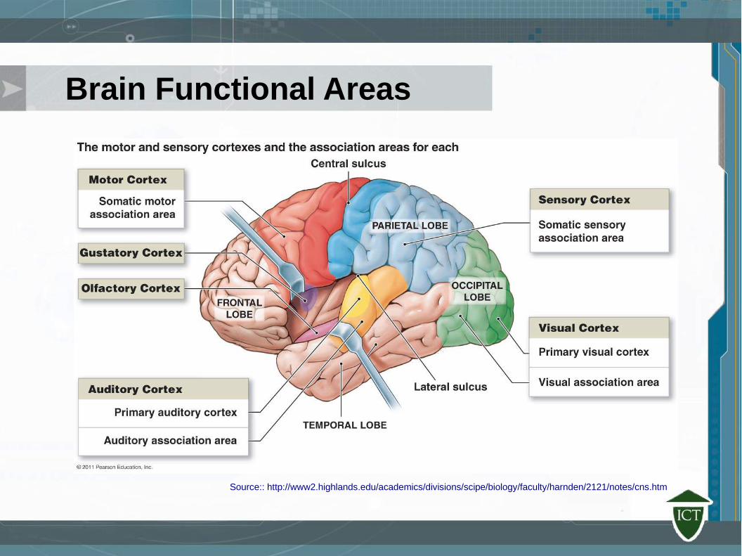
Brain Functional Areas
Source:: http://www2.highlands.edu/academics/divisions/scipe/biology/faculty/harnden/2121/notes/cns.htm
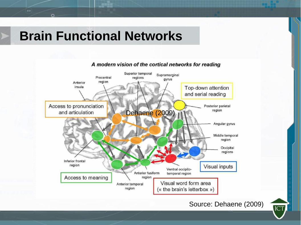
Brain Functional Networks
Dehaene (2009)
Source: Dehaene (2009)
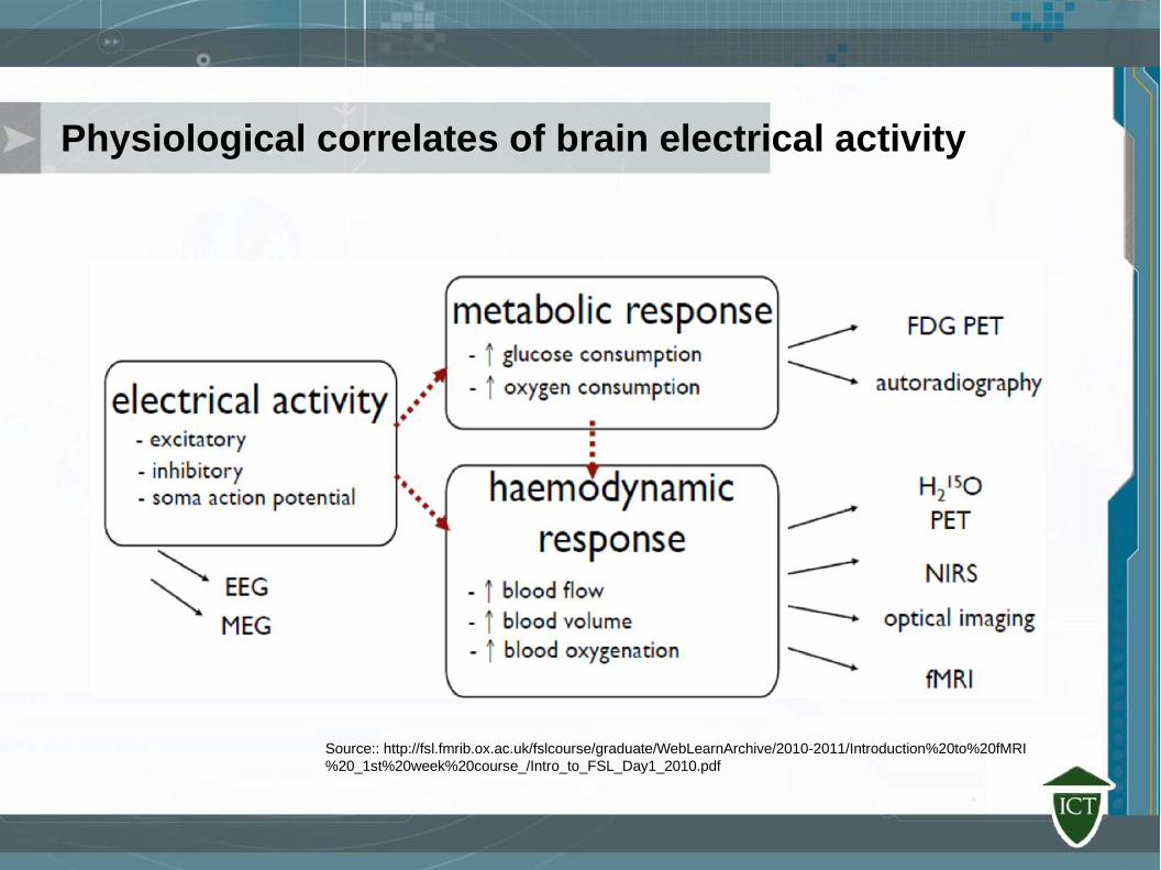
Physiological correlates of brain electrical activity
Source:: http://fsl.fmrib.ox.ac.uk/fslcourse/graduate/WebLearnArchive/2010-2011/Introduction%20to%20fMRI%20_1st%20week%20course_/Intro_to_FSL_Day1_2010.pdf
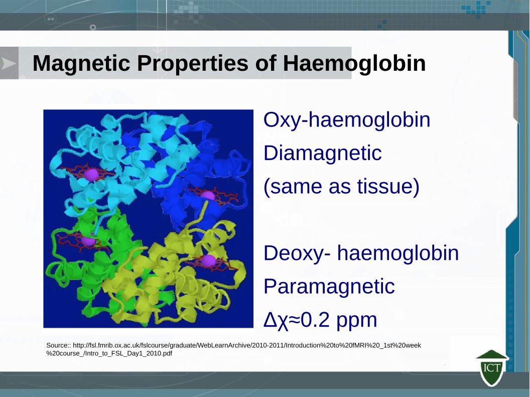
Magnetic Properties of Haemoglobin
Oxy-haemoglobin
Diamagnetic
(same as tissue)
Deoxy- haemoglobin
Paramagnetic
Δχ≈0.2 ppm Source:: http://fsl.fmrib.ox.ac.uk/fslcourse/graduate/WebLearnArchive/2010-2011/Introduction%20to%20fMRI%20_1st%20week%20course_/Intro_to_FSL_Day1_2010.pdf
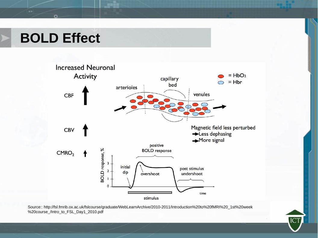
BOLD Effect
Source:: http://fsl.fmrib.ox.ac.uk/fslcourse/graduate/WebLearnArchive/2010-2011/Introduction%20to%20fMRI%20_1st%20week%20course_/Intro_to_FSL_Day1_2010.pdf
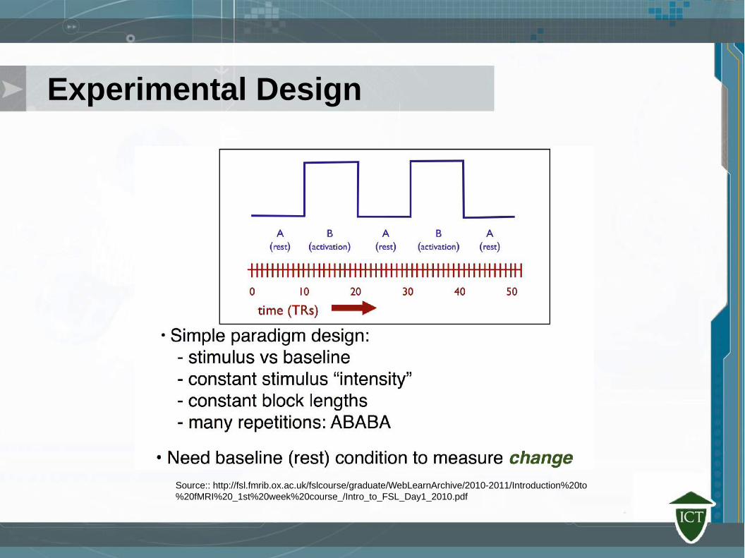
Experimental Design
Source:: http://fsl.fmrib.ox.ac.uk/fslcourse/graduate/WebLearnArchive/2010-2011/Introduction%20to%20fMRI%20_1st%20week%20course_/Intro_to_FSL_Day1_2010.pdf
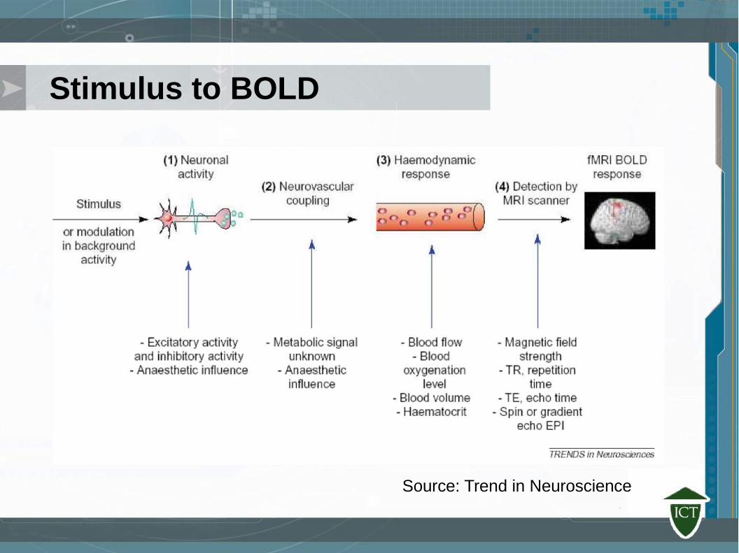
Stimulus to BOLD
Source: Trend in Neuroscience
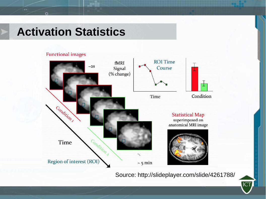
Activation Statistics
Source: http://slideplayer.com/slide/4261788/
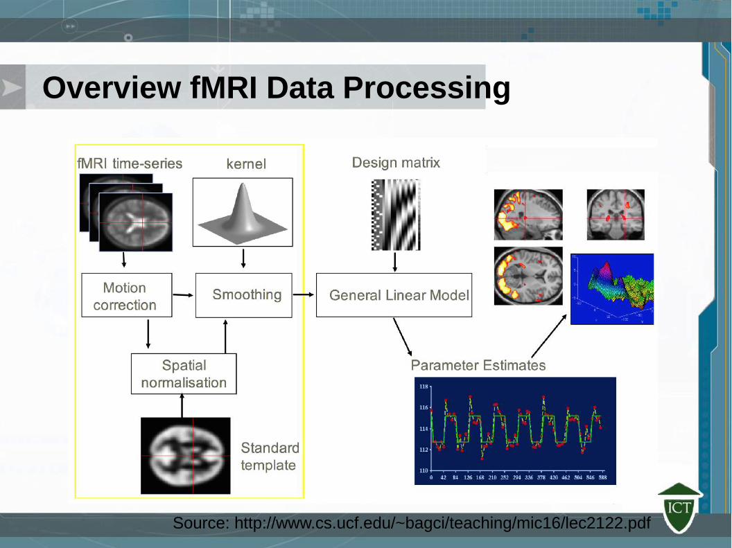
Overview fMRI Data Processing
Source: http://www.cs.ucf.edu/~bagci/teaching/mic16/lec2122.pdf
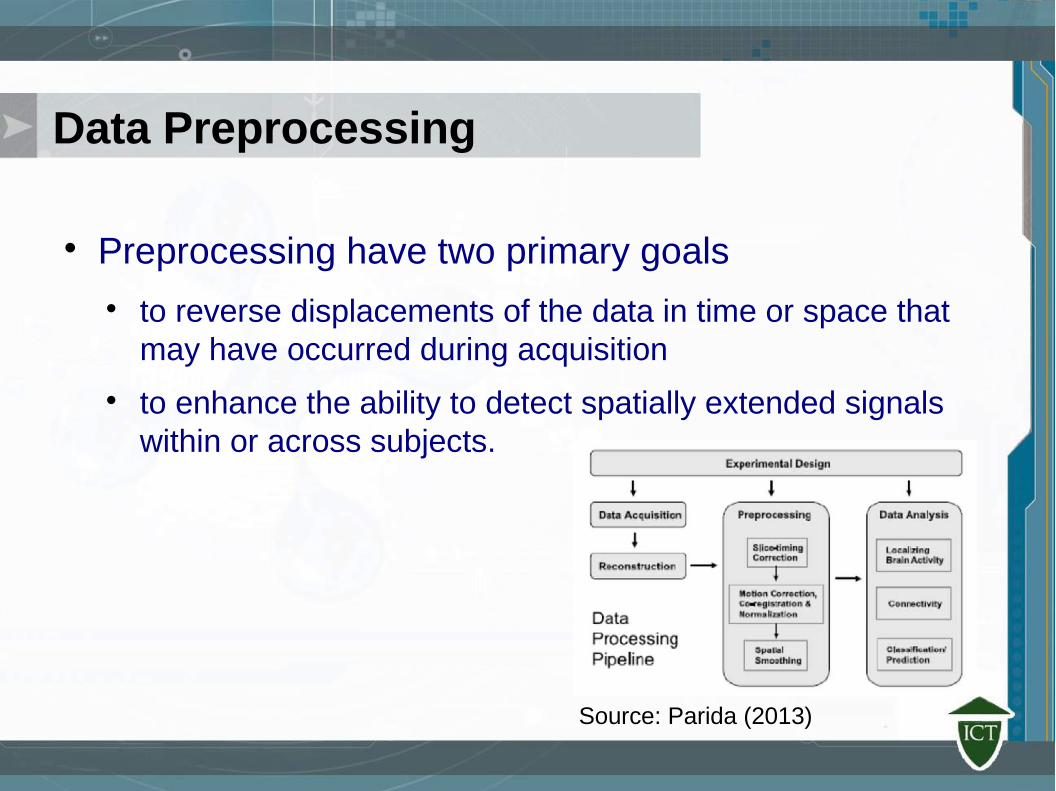
Data Preprocessing
Preprocessing have two primary goals to reverse displacements of the data in time or space that
may have occurred during acquisition
to enhance the ability to detect spatially extended signals within or across subjects.
Source: Parida (2013)
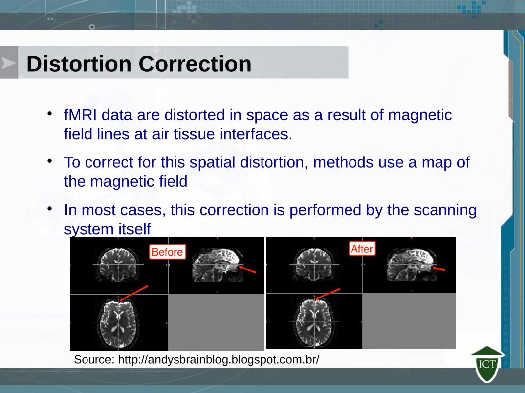
Distortion Correction
fMRI data are distorted in space as a result of magnetic field lines at air tissue interfaces.
To correct for this spatial distortion, methods use a map of the magnetic field
In most cases, this correction is performed by the scanning system itself
Source: http://andysbrainblog.blogspot.com.br/
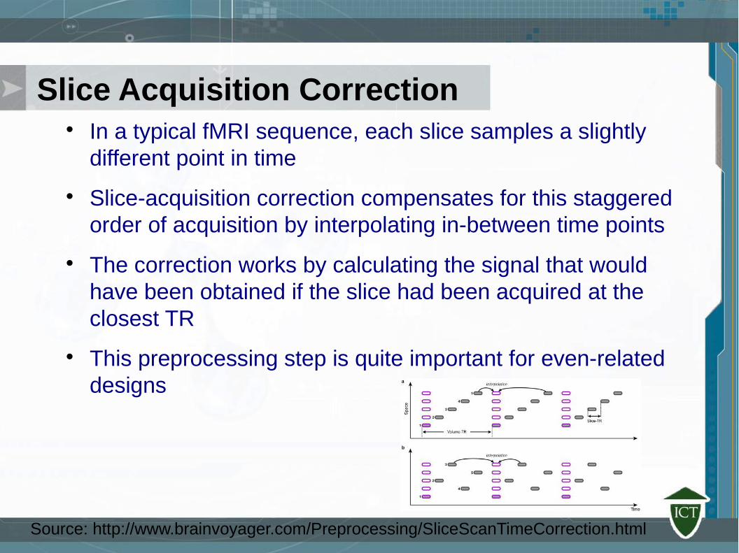
Slice Acquisition Correction In a typical fMRI sequence, each slice samples a slightly
different point in time
Slice-acquisition correction compensates for this staggered order of acquisition by interpolating in-between time points
The correction works by calculating the signal that would have been obtained if the slice had been acquired at the closest TR
This preprocessing step is quite important for even-related designs
Source: http://www.brainvoyager.com/Preprocessing/SliceScanTimeCorrection.html
Temporal High-Pass Filtering
The fMRI signal often show low-frequency drifts caused by physiological noise as well as by scanner-related noise these drifts reduce substantially the power of statistical
analysis invalidating event-related averaging
The removal of low-frequency drifts is one of the most important preprocessing steps and should be always performed This preprocessing can be "dangerous“ as condition-
related signals may be removed if correction is not properly applied

Motion Correction A common data preprocessing step is to correct for the effects
of motion by realigning the image of the brain obtained at each point in time back to the first or median image
Most methods treat the brain as a rigid body and calculate the six possible movement parameters which minimize the difference between the realigned brain and the brain in its reference position
Motion correction of this kind does not completely remove the effects of movement upon the fMRI signal
Statistical analysis of fMRI data often will consider the six movement parameters measured during realignment to account for changes in the signal within voxels that are correlated with the movement of the head
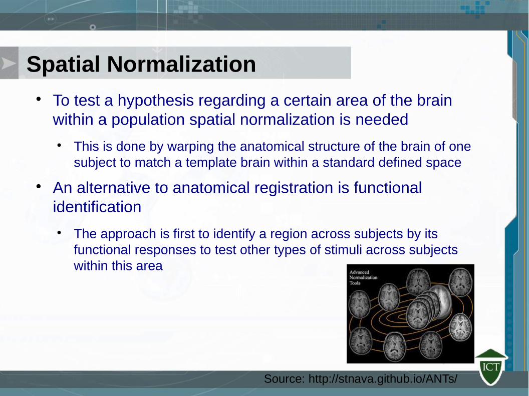
Spatial Normalization To test a hypothesis regarding a certain area of the brain
within a population spatial normalization is needed
This is done by warping the anatomical structure of the brain of one subject to match a template brain within a standard defined space
An alternative to anatomical registration is functional identification
The approach is first to identify a region across subjects by its functional responses to test other types of stimuli across subjects within this area
Source: http://stnava.github.io/ANTs/
References Faro, Scott H., and Feroze B. Mohamed, eds. BOLD fMRI: A guide to
functional imaging for neuroscientists. Springer Science & Business Media, 2010.
Parida, Shantipriya, and Satchidananda Dehuri. "Applying Machine Learning Techniques for Cognitive State Classification." IJCA Proceedings on International Conference in Distributed Computing and Internet Technology (ICDCIT), ICDCIT. 2013.