Embed Size (px)
Citation preview
Tutorials for Matlab and Pro/Engineering Wildfire 2.0
025.353 COMPUTER AIDED DESIGN AND ANALYSIS LABORATORY MANUALS
Instructor: Prof. Gary Wang
Dept. of Mechanical and Manufacturing Engineering The University of Manitoba
December 2004
MATLAB and Pro/E WILDFIRE 2.0 Tutorial
2
Contents 1. Introduction to MATLAB ........................................................................................................... 4
1.1 Objectives .............................................................................................................................. 4
1.2 Lab Requirement.................................................................................................................... 4
1.3 Background of MATLAB...................................................................................................... 4
1.4 The MATLAB System........................................................................................................... 4
1.5 Start of MATLAB.................................................................................................................. 5
1.6 Working Modes of MATLAB ............................................................................................... 6
1.7 Basic Commands ................................................................................................................... 6
1.8 Basic Operations .................................................................................................................... 9
1.9 An Example of Using MATLAB to Perform Geometric Transformation........................... 10
Lab 1: Generation of an Engineering Drawing Using MATLAB ............................................. 13
2. About the Pro/Engineer Wildfire 2.0 Tutorial .......................................................................... 15
2.1 What is Pro/ENGINEER?.................................................................................................. 15
2.2 Conventions Used in this Tutorial ....................................................................................... 15
3. Introduction to Pro/E WILDFIRE............................................................................................. 16
4. Modeling a Complete Part......................................................................................................... 28
4.1 Complete the Housing top ................................................................................................... 28
4.2 Build another extrusion: cylinder bracket............................................................................ 29
4.3 Build another extrusion: caliper bracket .............................................................................. 31
4.4 Create a cylinder .................................................................................................................. 32
4.6 Create the two chamfers....................................................................................................... 33
4.7 Create the rounds ................................................................................................................. 33
4.9 Clean your directory ............................................................................................................ 35
Lab 2 Part Modeling with Pro/Engineer ................................................................................... 36
5. Creating a 2-D Engineering Drawing........................................................................................ 38
5.1 Insert views .......................................................................................................................... 39
5.2 Add dimensions ................................................................................................................... 41
5.3 Other Useful Features .......................................................................................................... 43
Lab 3. Create a model and drawing ........................................................................................... 46

MATLAB and Pro/E WILDFIRE 2.0 Tutorial
3
6. Creating the Disk-Brake Assembly........................................................................................... 47
6.1 Six Common Assembly Constraints .................................................................................... 47
6.2 Build the disc-brake assembly ............................................................................................. 49
The final assembly show look like the following: ..................................................................... 52
6.3 Add Color and Create an Exploded View............................................................................ 52
6.4 Create a Cutout View........................................................................................................... 53
Lab 4 Assembly modeling ......................................................................................................... 55
7. Pro/Mechanica For Structural Analysis, Sensitivity Analysis, and Design Optimization ........ 56
7.1 Prepare the Model ................................................................................................................ 57
7.2 Start Pro/MECHANICA ...................................................................................................... 58
7.3 Define the FEA model ......................................................................................................... 58
7.4 Run a static analysis............................................................................................................. 59
7.5 Design parameter sensitivity study ...................................................................................... 63
7.6 Design optimization ............................................................................................................. 65
Lab 5 FEA Practice .................................................................................................................... 70
Appendix: Format of Reports........................................................................................................ 72
Format of the Laboratory Report ............................................................................................... 72
Format of the Project Report...................................................................................................... 72
MATLAB and Pro/E WILDFIRE 2.0 Tutorial
4
����������������� ������
1.1 Objectives To become familiar with the software MATLAB, and use it to perform numerical calculation and geometric transformations. This lab serves as the preparation step for Lab 1, which is the generation of engineering drawing using MATLAB.
1.2 Lab Requirement Students are required to read the manual, try the common commands listed in this manual on computer, and run the attached example in Section 0.
1.3 Background of MATLAB Originally developed to be a "matrix laboratory" by Cleve Moler, the recent versions that are written in C by the MathWorks Inc., have capabilities far beyond the original MATLAB. It is an interactive system and programming language for general scientific and technical computation. There are over 350 numeric and graphical functions available in the recent versions of MATLAB. Associated with it are several so-called toolboxes, each provides a fairly large set of additional commands that are of particular use for computing tasks in a specific engineering area such as control, system identification, digital signal processing, neural networks, optimization, etc. Together the MATLAB/Toolboxes package offers the user a powerful computing tool with superb graphics capabilities. More importantly, as MATLAB commands are similar to the way we express solution steps in mathematics, programming in MATLAB is much easier than its C or Fortran counterpart.
1.4 The MATLAB System
1. The MATLAB language. This is a high-level matrix/array language with control flow statements, functions, data structures, input/output, and object-oriented programming features. It allows both "programming in the small" to rapidly create quick and dirty throw-away programs, and "programming in the large" to create complete large and complex application programs.
2. The MATLAB working environment. This is the set of tools and facilities that you
work with as the MATLAB user or programmer. It includes facilities for managing the variables in your workspace and importing and exporting data. It also includes tools for developing, managing, debugging, and profiling M-files, MATLAB's applications.
3. Handle Graphics. This is the MATLAB graphics system. It includes high-level
commands for two-dimensional and three-dimensional data visualization, image processing, animation, and presentation graphics. It also includes low-level commands
MATLAB and Pro/E WILDFIRE 2.0 Tutorial
5
that allow you to fully customize the appearance of graphics as well as to build complete Graphical User Interfaces on your MATLAB applications (See Figure 1).
4. The MATLAB mathematical function library. This is a vast collection of
computational algorithms ranging from elementary functions like sum, sine, cosine, and complex arithmetic, to more sophisticated functions like matrix inverse, matrix eigenvalues, Bessel functions, and fast Fourier transforms.
5. The MATLAB Application Program Interface (API). This is a library that allows you
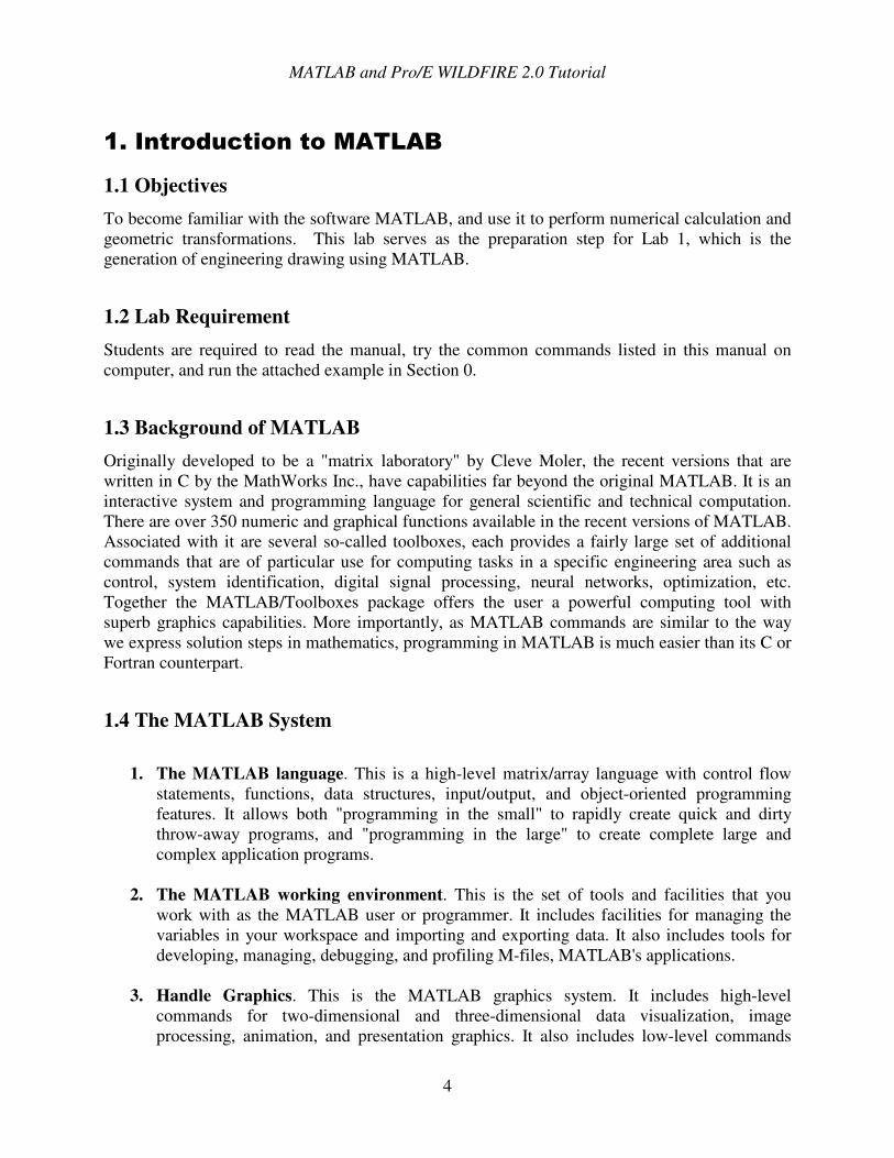
to write C and Fortran programs that interact with MATLAB. It includes facilities for calling routines from MATLAB (dynamic linking), calling MATLAB as a computational engine, and for reading and writing MAT-files. One can design customized graphical user interface (GUI) using Matlab language. Figure 1 shows an GUI developed in Matlab for performing optimization.
Figure 1 An example of a GUI developed using Matlab.
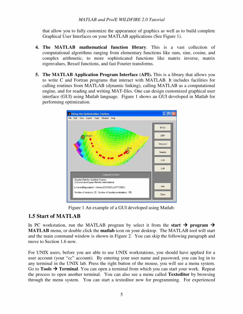
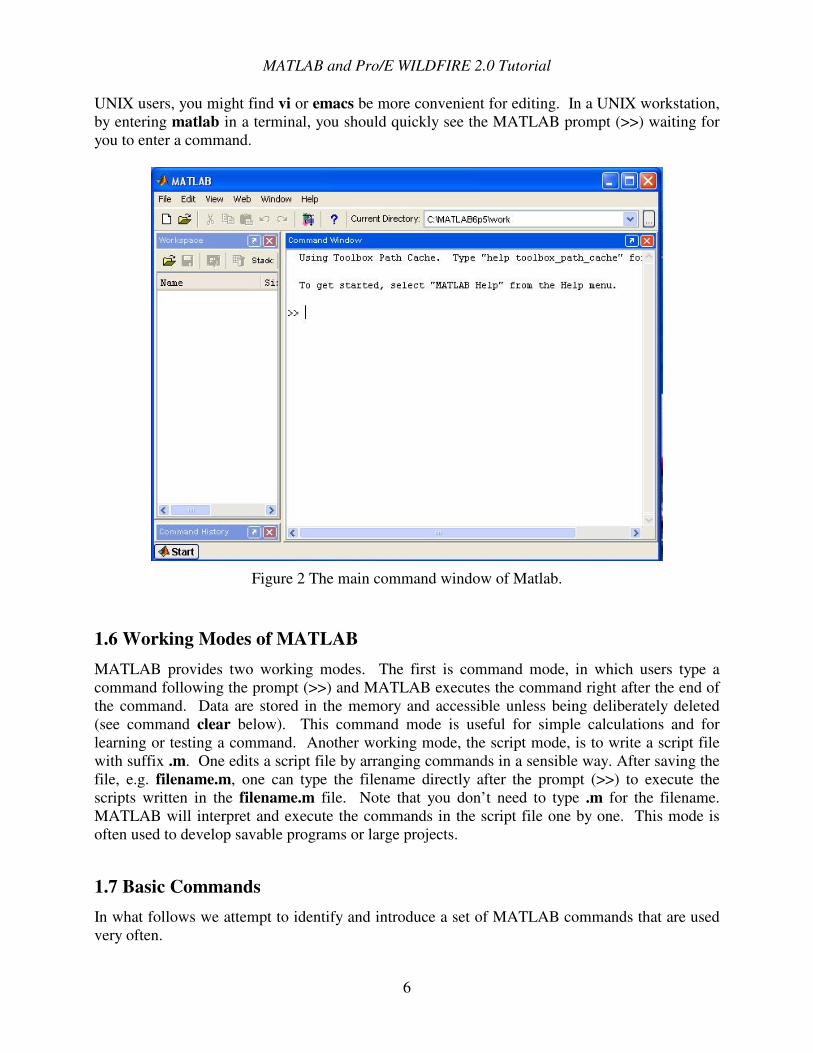
1.5 Start of MATLAB In PC workstation, run the MATLAB program by select it from the start ���� program ���� MATLAB menu, or double click the matlab icon on your desktop. The MATLAB tool will start and the main command window is shown in Figure 2. You can skip the following paragraph and move to Section 1.6 now. For UNIX users, before you are able to use UNIX workstations, you should have applied for a user account (your “cc” account). By entering your user name and password, you can log in to any terminal in the UNIX lab. Press the right button of the mouse, you will see a menu system. Go to Tools ���� Terminal. You can open a terminal from which you can start your work. Repeat the process to open another terminal. You can also see a menu called Texteditor by browsing through the menu system. You can start a texteditor now for programming. For experienced
MATLAB and Pro/E WILDFIRE 2.0 Tutorial
6
UNIX users, you might find vi or emacs be more convenient for editing. In a UNIX workstation, by entering matlab in a terminal, you should quickly see the MATLAB prompt (>>) waiting for you to enter a command.
Figure 2 The main command window of Matlab.
1.6 Working Modes of MATLAB MATLAB provides two working modes. The first is command mode, in which users type a command following the prompt (>>) and MATLAB executes the command right after the end of the command. Data are stored in the memory and accessible unless being deliberately deleted (see command clear below). This command mode is useful for simple calculations and for learning or testing a command. Another working mode, the script mode, is to write a script file with suffix .m. One edits a script file by arranging commands in a sensible way. After saving the file, e.g. filename.m, one can type the filename directly after the prompt (>>) to execute the scripts written in the filename.m file. Note that you don’t need to type .m for the filename. MATLAB will interpret and execute the commands in the script file one by one. This mode is often used to develop savable programs or large projects.
1.7 Basic Commands In what follows we attempt to identify and introduce a set of MATLAB commands that are used very often.
MATLAB and Pro/E WILDFIRE 2.0 Tutorial
7
1. Help functions If you need to know how to use a specific command, say plot, use command help plot. In case the explanation occupies more than one full screen page, you need to use more on which will cause MATLAB to pause after every screen full of information. You can type carriage return to continue. Type q while it is paused to exit out of displaying the current item. Also, more off disables automatic paging. If one doesn’t know the command or want to know more commands in a topic, use command help to see a list of help topics. You can then select the topic for which you want to have further information. Some of the topics are listed below:
HELP topics: matlab/general - General purpose commands. matlab/ops - Operators and special characters. matlab/lang - Programming language constructs. matlab/elmat - Elementary matrices and matrix manipulation. matlab/elfun - Elementary math functions. matlab/specfun - Specialized math functions. matlab/matfun - Matrix functions - numerical linear algebra. matlab/datafun - Data analysis and Fourier transforms. matlab/polyfun - Interpolation and polynomials. matlab/funfun - Function functions and ODE solvers. matlab/sparfun - Sparse matrices. matlab/graph2d - Two dimensional graphs. matlab/graph3d - Three dimensional graphs. matlab/specgraph - Specialized graphs. matlab/graphics - Handle Graphics. matlab/uitools - Graphical user interface tools. matlab/strfun - Character strings. matlab/iofun - File input/output. matlab/timefun - Time and dates. matlab/datatypes - Data types and structures. matlab/demos - Examples and demonstrations. … …
For more help on directory/topic, type "help topic". For instance, if you want to know all the matrix functions, type help matfun to view all the related commands. Another command is demo, which provides demo on each Matlab function. One can also use the Help menu on the Matlab window to access web resources.
2. Directory Operations
In a PC version, just simply press the directory icon in the left column as a standard WINDOWS operation. For UNIX users, to change current directory, one can use cd as in a UNIX terminal. The pwd command shows the current directory, and ls lists all the files in the current directory.
MATLAB and Pro/E WILDFIRE 2.0 Tutorial
8
3. Exit Matlab To exit MATLAB, use quit or exit.
4. Save Data in Matlab If you want to save some of the quantities that you have generated using MATLAB, say you want to save two matrices A, B and a vector c as a data file named data-01 for future use, use
save data-01 A B c
After that you will then find a file entitled data-0l.mat in your directory. Next time when you invoke the software again, use load data-01 to load the data you saved.
5. Abort a Command To abort a command in MATLAB, hold down the control key and then press the letter c.
6. Case Sensitivity Unless you have used command casesen off, MATLAB is case-sensitive. For example, the variable named dt, Dt, and DT are different from each other. Case sensitivity can be turned on and off with casesen that changes the case-sensitivity setting each time when the command is executed.
7. Memory Clean-up
MATLAB uses a command window to enter comments and data and to print results, and uses a graphics window to display plots. Use clf to clear the graphics window. To clear variables, say A and c, use command clear A c. Executing command clear only (without any specified variables following it) will delete all the variables generated.
8. Display Control
If one adds a comma at the end of a command, MATLAB will not generate any output for that command, if it generates some output. Otherwise, the output will be printed to the screen after the command. For example, if one types after the prompt (>>) A=3+4; MATLAB will generate no output and one will see another prompt after the command. If only A=3+4 is types, MATLAB will output A=7 on the screen. This feature is very useful in the script mode for users to control the program output.
9. Some Default Settings
By default, the angle unit in MATLAB is radian (Note you need to deal with angles in your first lab. Pay attention to this!). MATLAB also has pre-defined constant, pi, which can help you transfer the unit degree to radian.
MATLAB and Pro/E WILDFIRE 2.0 Tutorial
9
10. List Variables in Memory
The command who lists the variables that you have defined, while command whos lists the variables along with their sizes.
11. Print out
One can output a figure created by MATLAB to a file or a printer. For instance, one has generated a plot. In the command line, type print –djpeg filename.jpg and MATLAB will export the plot to the file filename.jpg as a graph. A variety of file types, besides jpeg file, can be generated in the same way. For detailed info, please use help print.
1.8 Basic Operations In this section we introduce more M-ATLAB commands for basic computations. Arithmetic operations
Example: Calculate (1+2)*(1+2)/(3-2)*2 The command in MATLAB will be >>(1+2)^2/(3-2)*2 18 >> Matrix operations
1. Define a matrix >> A = [1 2; 2 3; 3 4] A = 1 2
2 3 3 4
Transpose of matrix A >>A’ ans =
1 2 3 2 3 4
2. Check the size of a matrix >> size(A) ans =
3 2 >>size(A, 2) ans = 2
MATLAB and Pro/E WILDFIRE 2.0 Tutorial
10
The latter command refers to the number of columns of A. If size(A, 1), then the output will be 3, the number of rows. 3. Generate a matrix with all zeros and is of the same size of A >> B = zeros(size(A)) B =
0 0 0 0 0 0
4. Matrix reference To refer to the data on the third row and the second column in A, the command is >> A(3, 2) To refer to the first two rows of A >> A(1:2,:) To refer to the second column of A >> A(:, 2) 5. Matrix operations Matrix operations take the same form as basic arithmetic operations provided that all the matrices in the operations are of the same size, i.e., the same number of rows and columns.
Graphics Commands
• The most common graphics command is plot. Please type help plot in the MATLAB’s command window to see the detail description of the command.
• One can use hold on if multiple plots are expected to be printed in a same figure. Otherwise use hold off. The default setting of MATLAB is hold off.
• One can use the axis command to control the output data range. For example. Axis([-2 2 –3 3]) specifies that the x-coordinate between [-2 2] and the y-coordinate between [-3 3] will be printed.
• One can use title(‘your title’) to add a title to a plot. • Commands xlabel(‘your x label’) and ylabel(‘your y label’) add label to a 2-D plot.
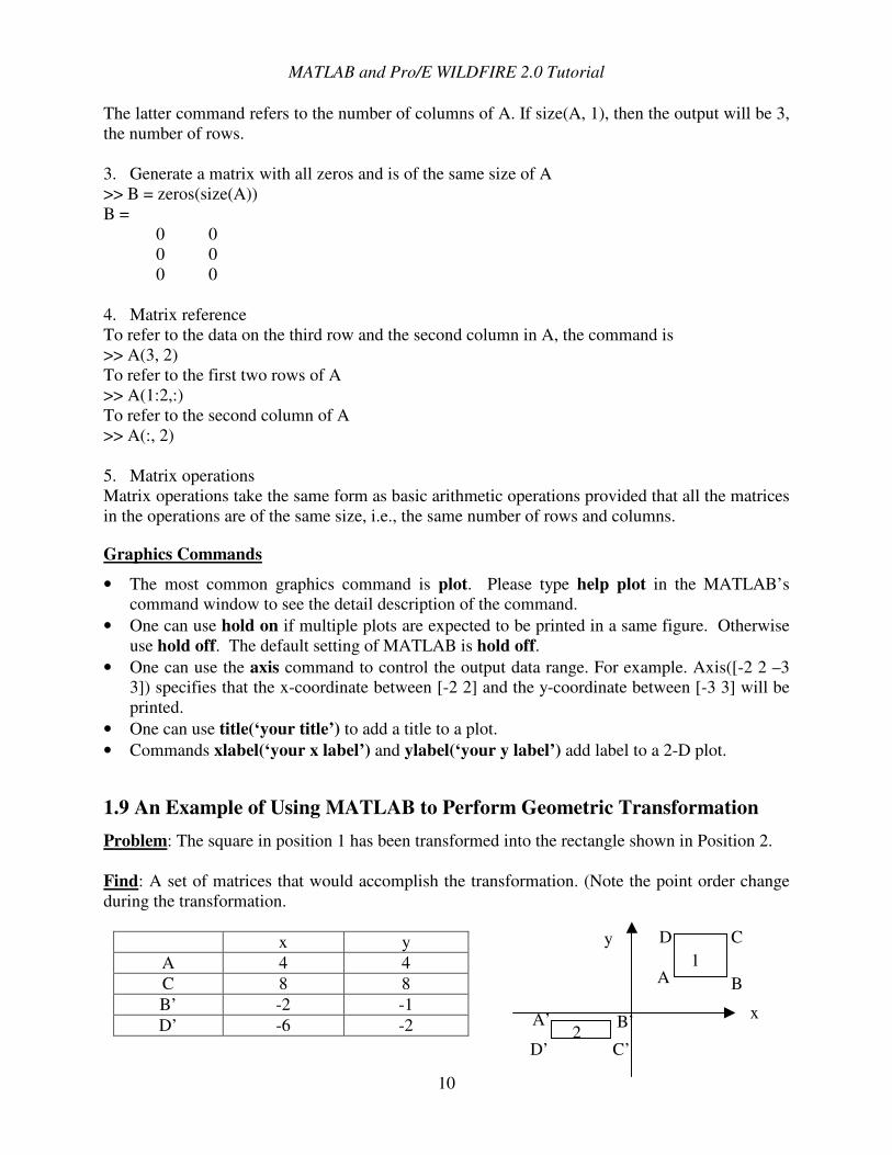
1.9 An Example of Using MATLAB to Perform Geometric Transformation Problem: The square in position 1 has been transformed into the rectangle shown in Position 2. Find: A set of matrices that would accomplish the transformation. (Note the point order change during the transformation.
x y A 4 4 C 8 8 B’ -2 -1 D’ -6 -2
B
C D
A
A’ B’
D’ C’
1
2 x
y
MATLAB and Pro/E WILDFIRE 2.0 Tutorial
11
Solution: Let’s assume that the point A of the square translates to the origin, then reflects with respect to x axis, scales down to the size of that in position 2, and finally translates to position 2. The program, written in MATLAB, is as follows. Students are encouraged to create a file, called Yourfilename.m, with the following content. Please note sentences that start with symbol “%” are comments. % ------------ Program starts here --------------- % MATLAB script file for the example % Date: 12/21/99 % Clear all the stored variables in memory. This is useful when you have multiple % script files running at the same time and these files might have variables with the % same name. clear; % T1 is for the first translation T1=[1 0 0 -4; 0 1 0 -4; 0 0 1 0; 0 0 0 1]; % reflection with respect to x axis REFx = [1 0 0 0; 0 -1 0 0; 0 0 1 0; 0 0 0 1]; % scale down S = [1 0 0 0; 0 0.25 0 0; 0 0 1 0; 0 0 0 1]; % the second translation T2 = [1 0 0 -6; 0 1 0 -1; 0 0 1 0; 0 0 0 1]; % The original point matrix, note that the last point repeats the first point % to make a closed box. P1 = [4 8 8 4 4; 4 4 8 8 4; 0 0 0 0 0; 1 1 1 1 1];
MATLAB and Pro/E WILDFIRE 2.0 Tutorial
12
% The resultant transformation matrix C = T2 * S * REFx * T1; % The point matrix of the rectangular in position 2 P2 = C * P1; % Prepare for plot clf; hold on; % plot grid grid on; % plot x and y axes as yellow lines plot([0,0],[-8, 8], ‘y’); plot([-8,8],[0,0],’y’); % plot box in original (red) and transformed (green) positions plot(P1(1,:), P1(2,:),’r’); plot(P2(1,:), P2(2,:),’g’); axis([-8 8 –8 8]); %specify the axis range % End the hold status hold off % ------------ Program ends here ------------------- Having created the file, save it as Yourfilename.m, then in the command window of MATLAB, type Yourfilename to execute it. If some error exists, MATLAB will prompt you on which line it hangs up. You can go back to the line in the script file to correct the error.
MATLAB and Pro/E WILDFIRE 2.0 Tutorial
13
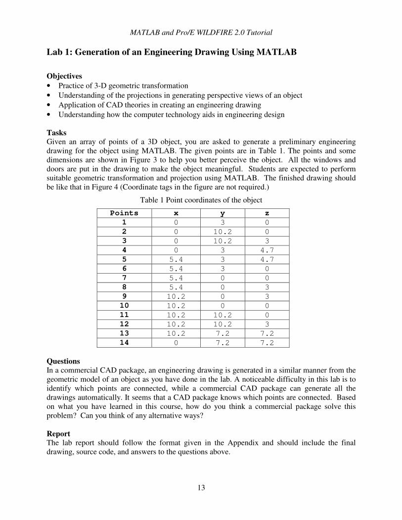
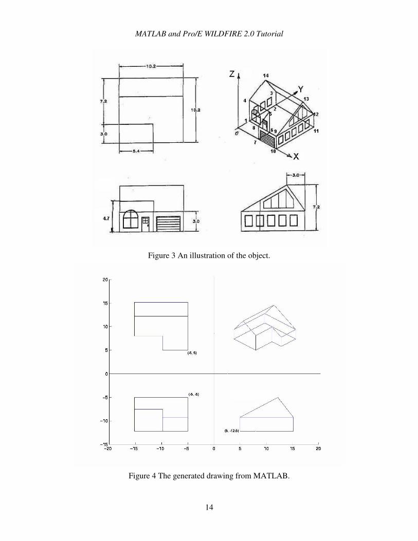
Lab 1: Generation of an Engineering Drawing Using MATLAB Objectives • Practice of 3-D geometric transformation • Understanding of the projections in generating perspective views of an object • Application of CAD theories in creating an engineering drawing • Understanding how the computer technology aids in engineering design Tasks Given an array of points of a 3D object, you are asked to generate a preliminary engineering drawing for the object using MATLAB. The given points are in Table 1. The points and some dimensions are shown in Figure 3 to help you better perceive the object. All the windows and doors are put in the drawing to make the object meaningful. Students are expected to perform suitable geometric transformation and projection using MATLAB. The finished drawing should be like that in Figure 4 (Coordinate tags in the figure are not required.)
Table 1 Point coordinates of the object
Points x y z 1 0 3 0 2 0 10.2 0 3 0 10.2 3 4 0 3 4.7 5 5.4 3 4.7 6 5.4 3 0 7 5.4 0 0 8 5.4 0 3 9 10.2 0 3 10 10.2 0 0 11 10.2 10.2 0 12 10.2 10.2 3 13 10.2 7.2 7.2 14 0 7.2 7.2
Questions In a commercial CAD package, an engineering drawing is generated in a similar manner from the geometric model of an object as you have done in the lab. A noticeable difficulty in this lab is to identify which points are connected, while a commercial CAD package can generate all the drawings automatically. It seems that a CAD package knows which points are connected. Based on what you have learned in this course, how do you think a commercial package solve this problem? Can you think of any alternative ways? Report The lab report should follow the format given in the Appendix and should include the final drawing, source code, and answers to the questions above.
MATLAB and Pro/E WILDFIRE 2.0 Tutorial
14
Figure 3 An illustration of the object.
Figure 4 The generated drawing from MATLAB.
MATLAB and Pro/E WILDFIRE 2.0 Tutorial
15
�������������������������� �������������������
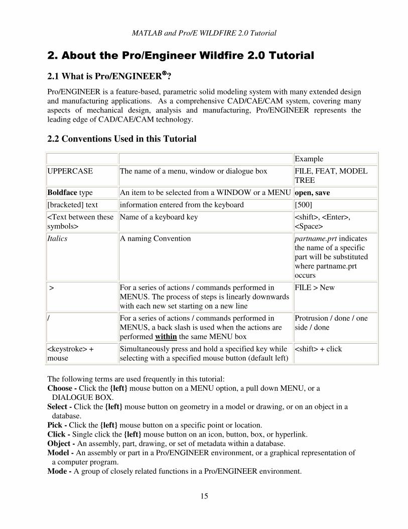
2.1 What is Pro/ENGINEER? Pro/ENGINEER is a feature-based, parametric solid modeling system with many extended design and manufacturing applications. As a comprehensive CAD/CAE/CAM system, covering many aspects of mechanical design, analysis and manufacturing, Pro/ENGINEER represents the leading edge of CAD/CAE/CAM technology. 2.2 Conventions Used in this Tutorial
The following terms are used frequently in this tutorial: Choose - Click the {left} mouse button on a MENU option, a pull down MENU, or a
DIALOGUE BOX. Select - Click the {left} mouse button on geometry in a model or drawing, or on an object in a
database. Pick - Click the {left} mouse button on a specific point or location. Click - Single click the {left} mouse button on an icon, button, box, or hyperlink. Object - An assembly, part, drawing, or set of metadata within a database. Model - An assembly or part in a Pro/ENGINEER environment, or a graphical representation of
a computer program. Mode - A group of closely related functions in a Pro/ENGINEER environment.
Example
UPPERCASE The name of a menu, window or dialogue box FILE, FEAT, MODEL TREE
Boldface type An item to be selected from a WINDOW or a MENU open, save
[bracketed] text information entered from the keyboard [500]
<Text between these symbols>
Name of a keyboard key <shift>, <Enter>, <Space>
Italics A naming Convention partname.prt indicates the name of a specific part will be substituted where partname.prt occurs
> For a series of actions / commands performed in MENUS. The process of steps is linearly downwards with each new set starting on a new line
FILE > New
/ For a series of actions / commands performed in MENUS, a back slash is used when the actions are performed within the same MENU box
Protrusion / done / one side / done
<keystroke> + mouse
Simultaneously press and hold a specified key while selecting with a specified mouse button (default left)
<shift> + click
MATLAB and Pro/E WILDFIRE 2.0 Tutorial
16
������������������������ �� !�"��
This chapter is intended to briefly explain the Pro/E User Interface and get you started with a simple modeling task. The steps needed to start Pro/E and to generate a part model is discussed in the following tutorials.
Starting Pro/E
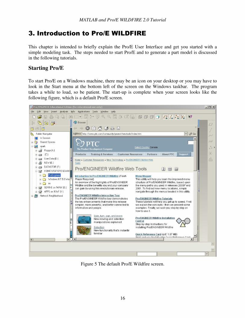
To start Pro/E on a Windows machine, there may be an icon on your desktop or you may have to look in the Start menu at the bottom left of the screen on the Windows taskbar. The program takes a while to load, so be patient. The start-up is complete when your screen looks like the following figure, which is a default Pro/E screen.
Figure 5 The default Pro/E Wildfire screen.
MATLAB and Pro/E WILDFIRE 2.0 Tutorial
17
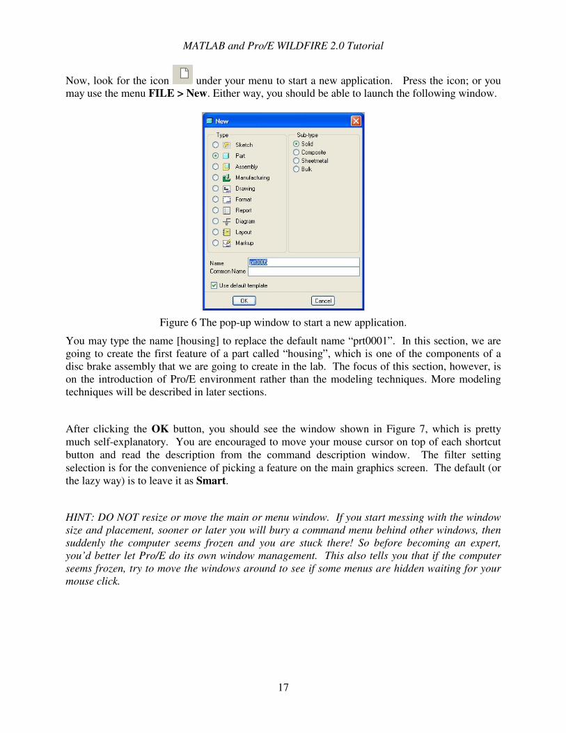
Now, look for the icon under your menu to start a new application. Press the icon; or you may use the menu FILE > New. Either way, you should be able to launch the following window.
Figure 6 The pop-up window to start a new application.
You may type the name [housing] to replace the default name “prt0001”. In this section, we are going to create the first feature of a part called “housing”, which is one of the components of a disc brake assembly that we are going to create in the lab. The focus of this section, however, is on the introduction of Pro/E environment rather than the modeling techniques. More modeling techniques will be described in later sections.
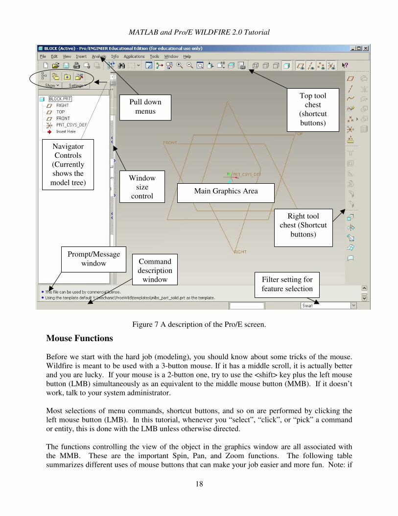
After clicking the OK button, you should see the window shown in Figure 7, which is pretty much self-explanatory. You are encouraged to move your mouse cursor on top of each shortcut button and read the description from the command description window. The filter setting selection is for the convenience of picking a feature on the main graphics screen. The default (or the lazy way) is to leave it as Smart.
HINT: DO NOT resize or move the main or menu window. If you start messing with the window size and placement, sooner or later you will bury a command menu behind other windows, then suddenly the computer seems frozen and you are stuck there! So before becoming an expert, you’d better let Pro/E do its own window management. This also tells you that if the computer seems frozen, try to move the windows around to see if some menus are hidden waiting for your mouse click.
MATLAB and Pro/E WILDFIRE 2.0 Tutorial
18
Figure 7 A description of the Pro/E screen.
Mouse Functions Before we start with the hard job (modeling), you should know about some tricks of the mouse. Wildfire is meant to be used with a 3-button mouse. If it has a middle scroll, it is actually better and you are lucky. If your mouse is a 2-button one, try to use the <shift> key plus the left mouse button (LMB) simultaneously as an equivalent to the middle mouse button (MMB). If it doesn’t work, talk to your system administrator. Most selections of menu commands, shortcut buttons, and so on are performed by clicking the left mouse button (LMB). In this tutorial, whenever you “select”, “click”, or “pick” a command or entity, this is done with the LMB unless otherwise directed. The functions controlling the view of the object in the graphics window are all associated with the MMB. These are the important Spin, Pan, and Zoom functions. The following table summarizes different uses of mouse buttons that can make your job easier and more fun. Note: if
Main Graphics Area
Navigator Controls
(Currently shows the
model tree)
Prompt/Message window Command
description window
Pull down menus
Right tool chest (Shortcut
buttons)
Top tool chest
(shortcut buttons)
Filter setting for feature selection
Window size
control
MATLAB and Pro/E WILDFIRE 2.0 Tutorial
19
you know previous versions of Pro/E, you will find the mouse functions are quite different! Learn the new functions and don’t let your experience frustrate you.
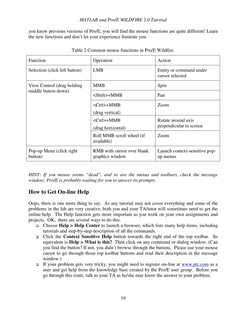
Table 2 Common mouse functions in Pro/E Wildfire.
Function Operation Action
Selection (click left button) LMB Entity or command under cursor selected
MMB Spin
<Shift>+MMB Pan
<Ctrl>+MMB
(drag vertical)
Zoom
<Ctrl>+MMB
(drag horizontal)
Rotate around axis perpendicular to screen
View Control (drag holding middle button down)
Roll MMB scroll wheel (if available)
Zoom
Pop-up Menu (click right button)
RMB with cursor over blank graphics window
Launch context-sensitive pop-up menus
HINT: If you mouse seems “dead”, and so are the menus and toolbars, check the message window; Pro/E is probably waiting for you to answer its prompts. How to Get On-line Help Oops, there is one more thing to say. As any tutorial may not cover everything and some of the problems in the lab are very creative, both you and your TA/tutor will sometimes need to get the online-help. The Help function gets more important as you work on your own assignments and projects. OK, there are several ways to do this.
�� Choose Help > Help Center to launch a browser, which lists many help items, including tutorials and step-by-step description of all the commands.
�� Click the Context Sensitive Help button towards the right end of the top toolbar. Its equivalent is Help > What is this?. Then click on any command or dialog window. (Can you find the button? If not, you didn’t browse through the buttons. Please use your mouse cursor to go through those top toolbar buttons and read their description in the message window.)
�� If your problem gets very tricky, you might need to register on-line at www.ptc.com as a user and get help from the knowledge base created by the Pro/E user group. Before you go through this route, talk to your TA as he/she may know the answer to your problem.
MATLAB and Pro/E WILDFIRE 2.0 Tutorial
20
Begin to work in Pro/E Now back to Figure 7 where we left off. The left side of the main window shows the model tree of the empty part “housing”. The main graphics windows shows three orthogonal planes, named TOP, FRONT and RIGHT, and a coordinate system. These planes are called datum planes, representing the 3-D world. These planes are very useful as reference planes when creating features and assembling components. Their advantages are not obvious when modeling simple parts, and in fact new users find these planes annoying. Whatever you feel now, my advice is to get yourself used to these “annoying” planes.
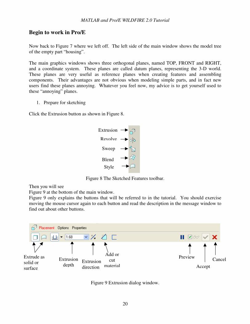
1. Prepare for sketching Click the Extrusion button as shown in Figure 8.
Figure 8 The Sketched Features toolbar.
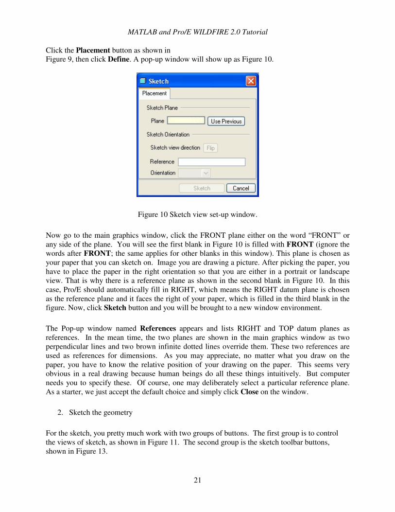
Then you will see Figure 9 at the bottom of the main window. Figure 9 only explains the buttons that will be referred to in the tutorial. You should exercise moving the mouse cursor again to each button and read the description in the message window to find out about other buttons.
Figure 9 Extrusion dialog window.
Extrusion
Revolve
Sweep
Blend Style
Extrusion depth
Extrusion direction
Add or cut
material
Preview
Accept Cancel Extrude as
solid or surface
MATLAB and Pro/E WILDFIRE 2.0 Tutorial
21
Click the Placement button as shown in Figure 9, then click Define. A pop-up window will show up as Figure 10.
Figure 10 Sketch view set-up window.
Now go to the main graphics window, click the FRONT plane either on the word “FRONT” or any side of the plane. You will see the first blank in Figure 10 is filled with FRONT (ignore the words after FRONT; the same applies for other blanks in this window). This plane is chosen as your paper that you can sketch on. Image you are drawing a picture. After picking the paper, you have to place the paper in the right orientation so that you are either in a portrait or landscape view. That is why there is a reference plane as shown in the second blank in Figure 10. In this case, Pro/E should automatically fill in RIGHT, which means the RIGHT datum plane is chosen as the reference plane and it faces the right of your paper, which is filled in the third blank in the figure. Now, click Sketch button and you will be brought to a new window environment.
The Pop-up window named References appears and lists RIGHT and TOP datum planes as references. In the mean time, the two planes are shown in the main graphics window as two perpendicular lines and two brown infinite dotted lines override them. These two references are used as references for dimensions. As you may appreciate, no matter what you draw on the paper, you have to know the relative position of your drawing on the paper. This seems very obvious in a real drawing because human beings do all these things intuitively. But computer needs you to specify these. Of course, one may deliberately select a particular reference plane. As a starter, we just accept the default choice and simply click Close on the window.
2. Sketch the geometry
For the sketch, you pretty much work with two groups of buttons. The first group is to control the views of sketch, as shown in Figure 11. The second group is the sketch toolbar buttons, shown in Figure 13.
MATLAB and Pro/E WILDFIRE 2.0 Tutorial
22
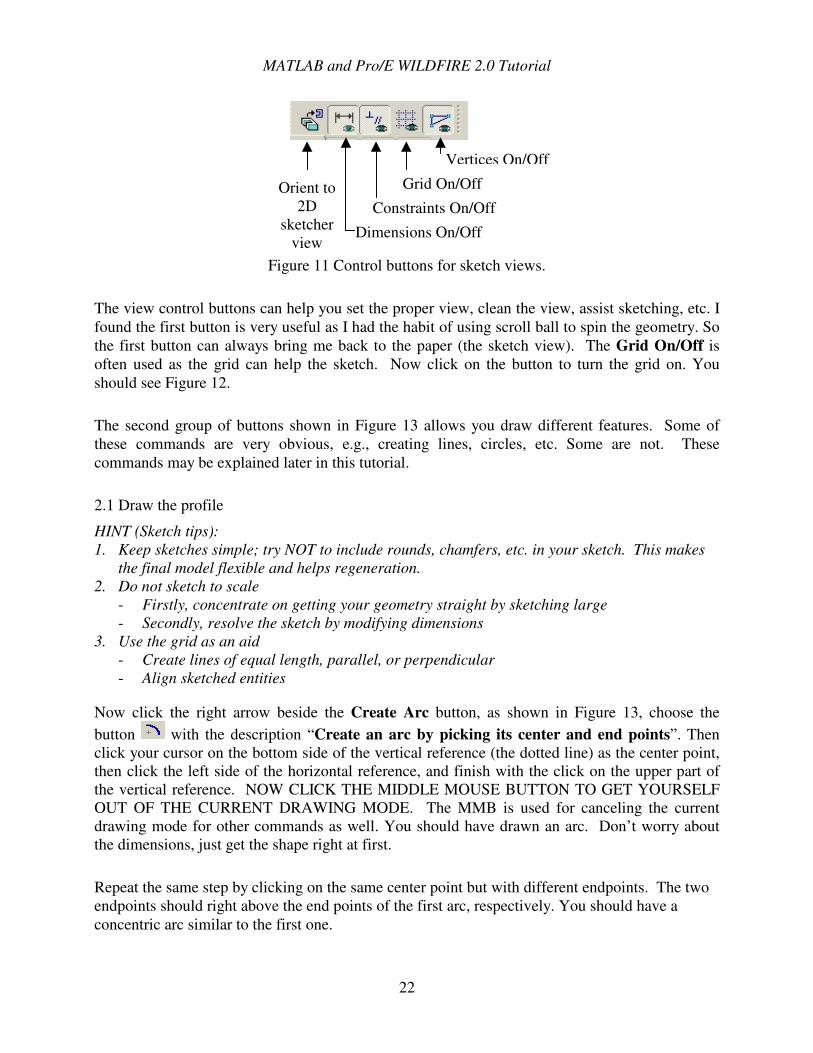
Figure 11 Control buttons for sketch views.
The view control buttons can help you set the proper view, clean the view, assist sketching, etc. I found the first button is very useful as I had the habit of using scroll ball to spin the geometry. So the first button can always bring me back to the paper (the sketch view). The Grid On/Off is often used as the grid can help the sketch. Now click on the button to turn the grid on. You should see Figure 12.
The second group of buttons shown in Figure 13 allows you draw different features. Some of these commands are very obvious, e.g., creating lines, circles, etc. Some are not. These commands may be explained later in this tutorial.
2.1 Draw the profile
HINT (Sketch tips): 1. Keep sketches simple; try NOT to include rounds, chamfers, etc. in your sketch. This makes
the final model flexible and helps regeneration. 2. Do not sketch to scale
- Firstly, concentrate on getting your geometry straight by sketching large - Secondly, resolve the sketch by modifying dimensions
3. Use the grid as an aid - Create lines of equal length, parallel, or perpendicular - Align sketched entities
Now click the right arrow beside the Create Arc button, as shown in Figure 13, choose the button with the description “Create an arc by picking its center and end points”. Then click your cursor on the bottom side of the vertical reference (the dotted line) as the center point, then click the left side of the horizontal reference, and finish with the click on the upper part of the vertical reference. NOW CLICK THE MIDDLE MOUSE BUTTON TO GET YOURSELF OUT OF THE CURRENT DRAWING MODE. The MMB is used for canceling the current drawing mode for other commands as well. You should have drawn an arc. Don’t worry about the dimensions, just get the shape right at first.
Repeat the same step by clicking on the same center point but with different endpoints. The two endpoints should right above the end points of the first arc, respectively. You should have a concentric arc similar to the first one.
Orient to 2D
sketcher view
Dimensions On/Off
Constraints On/Off
Grid On/Off
Vertices On/Off
MATLAB and Pro/E WILDFIRE 2.0 Tutorial
23
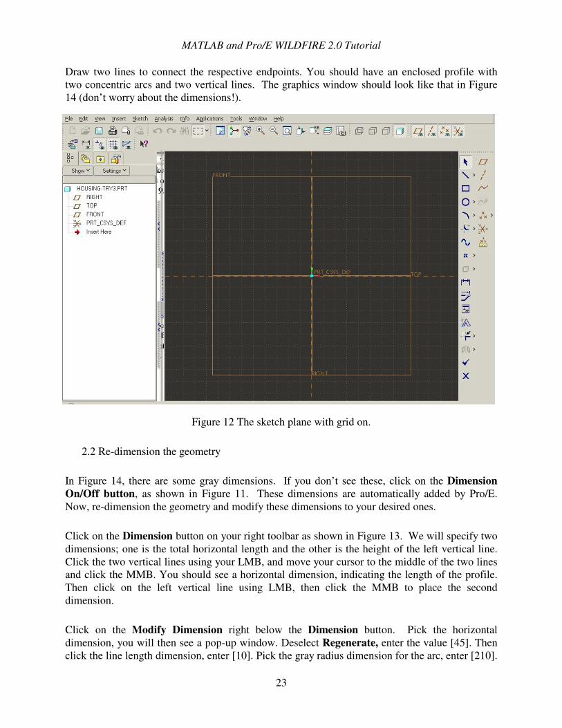
Draw two lines to connect the respective endpoints. You should have an enclosed profile with two concentric arcs and two vertical lines. The graphics window should look like that in Figure 14 (don’t worry about the dimensions!).
Figure 12 The sketch plane with grid on.
2.2 Re-dimension the geometry
In Figure 14, there are some gray dimensions. If you don’t see these, click on the Dimension On/Off button, as shown in Figure 11. These dimensions are automatically added by Pro/E. Now, re-dimension the geometry and modify these dimensions to your desired ones.
Click on the Dimension button on your right toolbar as shown in Figure 13. We will specify two dimensions; one is the total horizontal length and the other is the height of the left vertical line. Click the two vertical lines using your LMB, and move your cursor to the middle of the two lines and click the MMB. You should see a horizontal dimension, indicating the length of the profile. Then click on the left vertical line using LMB, then click the MMB to place the second dimension.
Click on the Modify Dimension right below the Dimension button. Pick the horizontal dimension, you will then see a pop-up window. Deselect Regenerate, enter the value [45]. Then click the line length dimension, enter [10]. Pick the gray radius dimension for the arc, enter [210].
MATLAB and Pro/E WILDFIRE 2.0 Tutorial
24
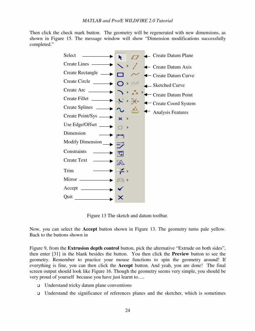
Then click the check mark button. The geometry will be regenerated with new dimensions, as shown in Figure 15. The message window will show “Dimension modifications successfully completed.”
Figure 13 The sketch and datum toolbar.
Now, you can select the Accept button shown in Figure 13. The geometry turns pale yellow. Back to the buttons shown in
Figure 9, from the Extrusion depth control button, pick the alternative “Extrude on both sides”, then enter [31] in the blank besides the button. You then click the Preview button to see the geometry. Remember to practice your mouse functions to spin the geometry around! If everything is fine, you can then click the Accept button. And yeah, you are done! The final screen output should look like Figure 16. Though the geometry seems very simple, you should be very proud of yourself because you have just learnt to….
�� Understand tricky datum plane conventions
�� Understand the significance of references planes and the sketcher, which is sometimes
Select
Create Lines
Create Rectangle
Create Circle
Create Arc
Create Fillet
Create Splines
Create Point/Sys
Use Edge/Offset
Dimension
Modify Dimension
Constraints
Create Text Trim
Mirror
Accept
Quit
Create Datum Plane Create Datum Axis
Create Datum Curve
Sketched Curve
Create Datum Point
Create Coord System
Analysis Features
MATLAB and Pro/E WILDFIRE 2.0 Tutorial
25
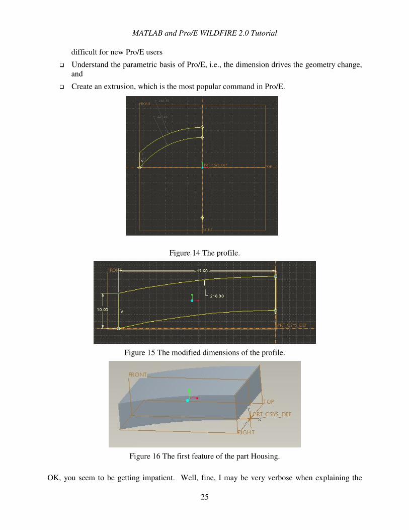
difficult for new Pro/E users
�� Understand the parametric basis of Pro/E, i.e., the dimension drives the geometry change, and
�� Create an extrusion, which is the most popular command in Pro/E.
Figure 14 The profile.
Figure 15 The modified dimensions of the profile.
Figure 16 The first feature of the part Housing.
OK, you seem to be getting impatient. Well, fine, I may be very verbose when explaining the
MATLAB and Pro/E WILDFIRE 2.0 Tutorial
26
first feature. After that, this tutorial will become sketchy and sloppy. Please be patient with me since the first is always the hardest, and you won’t be able to enjoy this detailed information before long. Also if you want save time at the beginning, you might end up spending more later.
3. Redefine the feature In case you messed up the part and cannot get the one shown in Figure 16. Don’t panic. Click the Extrude 1 feature (or even the sketch feature under this extrusion feature) in your Model tree window using the RMB. You will then see a bunch of commands including Edit, Edit Definition, etc. The Edit command allows you modify dimensions in 3D mode and the Edit Definition command brings you back to the sketch and the extrusion definition environment. You can then correct the steps that have been messed up with and follow the instructions in this section to get it right. Another way to modify a dimension is to double click a feature in the main graphics window; all the dimensions relevant to the feature will show up. You can double click the dimension you want to modify and enter a new number. Then click the Regenerates Model button (To use this function, make sure the Filter Setting at the right bottom corner of the window is turned to Features.).
4. Save, view, and print the model Pro/E, unlike other Windows applications, does not automatically save your work. You have to remember to do that. If you leave the program without saving your new work, it is basically gone! Anyone who says that they have never lost work this way is probably lying! Click FILE> Set Working Directory to change the default directory to a subdirectory under your home C:\25.353\start directory. By doing this, you can keep the default Pro/E directory tidy and avoid someone else accidentally deleting your file. HINT: Save your model frequently to avoid loss of work. Now, you should play with the buttons in the top tool chest.
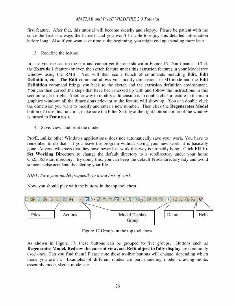
Figure 17 Groups in the top tool chest.
As shown in Figure 17, these buttons can be grouped to five groups. Buttons such as Regenerates Model, Redraw the current view, and Refit object to fully display are commonly used ones. Can you find them? Please note these toolbar buttons will change, depending which mode you are in. Examples of different modes are part modeling model, drawing mode, assembly mode, sketch mode, etc.
Files Actions Group
Model Display Group
Datum Help

MATLAB and Pro/E WILDFIRE 2.0 Tutorial
27
You can use FILE > Print to print your model, or FILE > Save a Copy to print it as a picture or formats readable by other CAD tools. Or, you could simply use the <Print Scrn> key on your keyboard and then use Microsoft Paint to convert it into a picture file.
MATLAB and Pro/E WILDFIRE 2.0 Tutorial
28
#�� ���������$�% &�����������
OK, assuming you
�� Have familiarized yourself with the Pro/E environment and you did either view and/or try all the buttons, icons, etc.
�� have built the first feature alright, and
�� can build the first feature again without reading the tutorial
If the answers to all the above are YES, then move on. Otherwise, go back to the previous chapter until the answers are YES. Because the rest of tutorial will be sketchy and, maybe, sloppy. You will be very frustrated if you didn’t do the first chapter well.
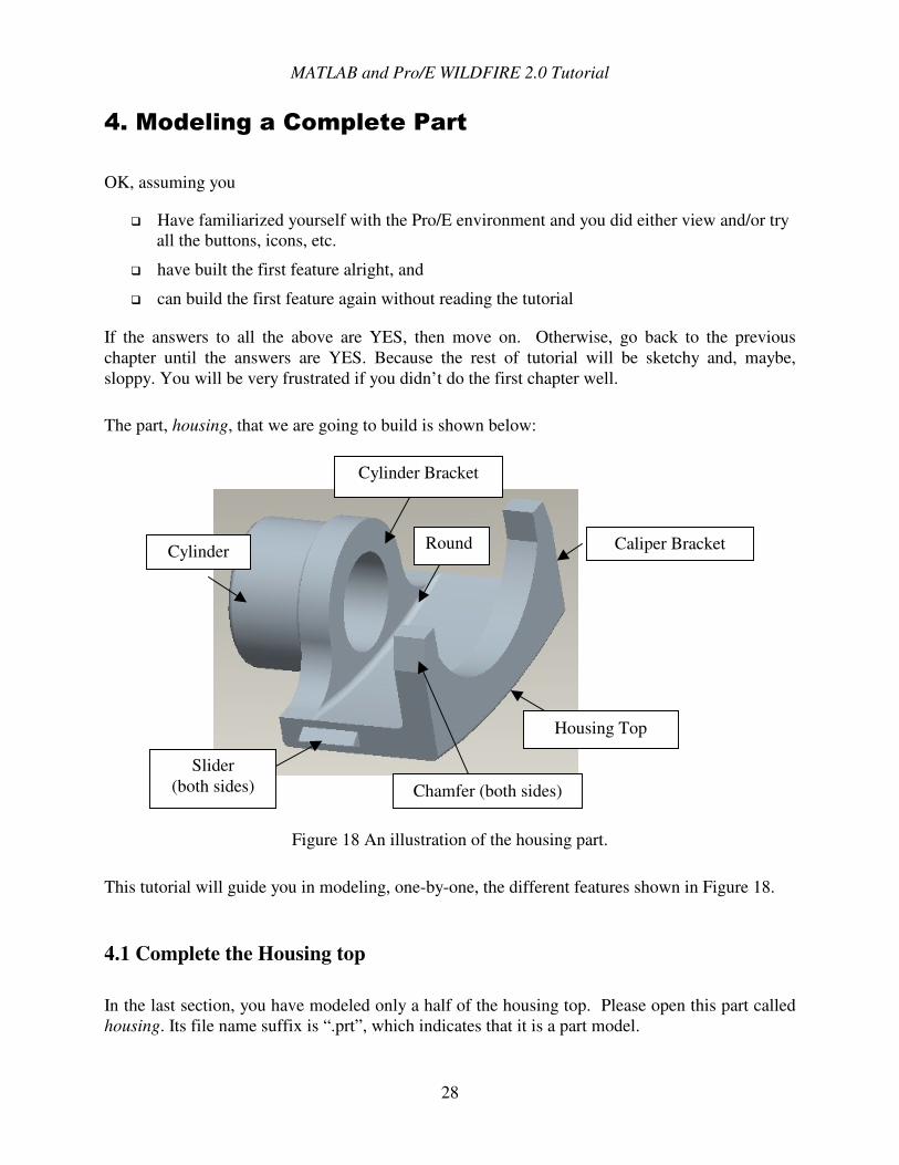
The part, housing, that we are going to build is shown below:
Figure 18 An illustration of the housing part.
This tutorial will guide you in modeling, one-by-one, the different features shown in Figure 18.
4.1 Complete the Housing top
In the last section, you have modeled only a half of the housing top. Please open this part called housing. Its file name suffix is “.prt”, which indicates that it is a part model.
Housing Top
Cylinder Bracket
Caliper Bracket Cylinder
Slider (both sides) Chamfer (both sides)
Rounds
MATLAB and Pro/E WILDFIRE 2.0 Tutorial
29
We are going to model the other half of the feature by performing a command called “mirror”. The logic of the action is 1) pick the feature to be mirrored, and 2) pick the “mirror”.
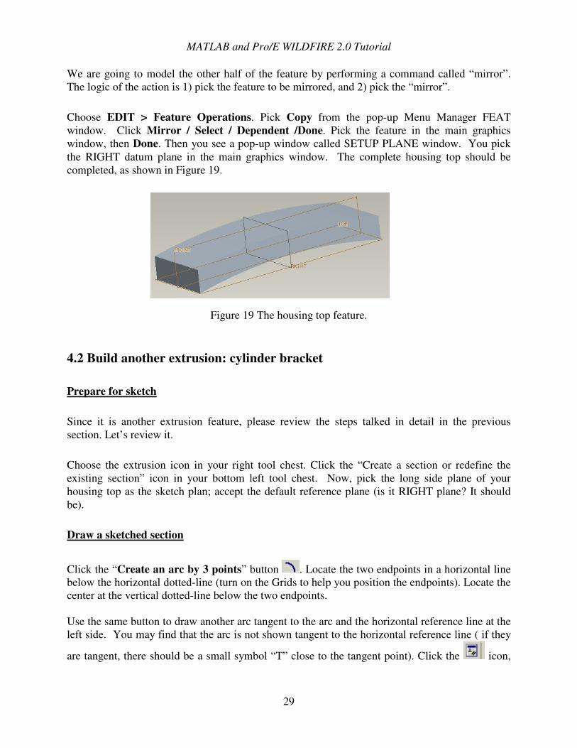
Choose EDIT > Feature Operations. Pick Copy from the pop-up Menu Manager FEAT window. Click Mirror / Select / Dependent /Done. Pick the feature in the main graphics window, then Done. Then you see a pop-up window called SETUP PLANE window. You pick the RIGHT datum plane in the main graphics window. The complete housing top should be completed, as shown in Figure 19.
Figure 19 The housing top feature.
4.2 Build another extrusion: cylinder bracket
Prepare for sketch
Since it is another extrusion feature, please review the steps talked in detail in the previous section. Let’s review it.
Choose the extrusion icon in your right tool chest. Click the “Create a section or redefine the existing section” icon in your bottom left tool chest. Now, pick the long side plane of your housing top as the sketch plan; accept the default reference plane (is it RIGHT plane? It should be).
Draw a sketched section
Click the “Create an arc by 3 points” button . Locate the two endpoints in a horizontal line below the horizontal dotted-line (turn on the Grids to help you position the endpoints). Locate the center at the vertical dotted-line below the two endpoints.
Use the same button to draw another arc tangent to the arc and the horizontal reference line at the left side. You may find that the arc is not shown tangent to the horizontal reference line ( if they
are tangent, there should be a small symbol “T” close to the tangent point). Click the icon,
MATLAB and Pro/E WILDFIRE 2.0 Tutorial
30
then pick the . Select the new arc and the horizontal line. The small “T” should show up. This means the two entities are now tangent. Then dimension the two arcs as shown in Figure 20. Draw a line to connect the tangent point with the left bottom point of the housing top feature. In this exercise, we are going to practice using the “mirror” tool in sketch mode. First you should sketch a centreline which represents the “mirror” plane. Find and click the “Create 2 point
centreline” button and draw a line coinciding with the vertical dotted-line (remember what is this?). Pick the new arc and the line (hold the <ctrl> key for multiple selection). Then click the mirror icon . These two entities should be copied to the right hand side.
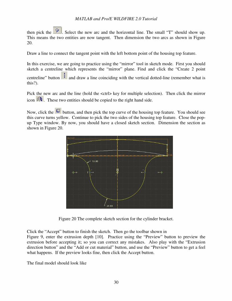
Now, click the button, and then pick the top curve of the housing top feature. You should see this curve turns yellow. Continue to pick the two sides of the housing top feature. Close the pop-up Type window. By now, you should have a closed sketch section. Dimension the section as shown in Figure 20.
Figure 20 The complete sketch section for the cylinder bracket.
Click the “Accept” button to finish the sketch. Then go the toolbar shown in Figure 9, enter the extrusion depth [10]. Practice using the “Preview” button to preview the extrusion before accepting it; so you can correct any mistakes. Also play with the “Extrusion direction button” and the “Add or cut material” button, and use the “Preview” button to get a feel what happens. If the preview looks fine, then click the Accept button. The final model should look like
MATLAB and Pro/E WILDFIRE 2.0 Tutorial
31
Figure 21 The housing top and the cylinder bracket.
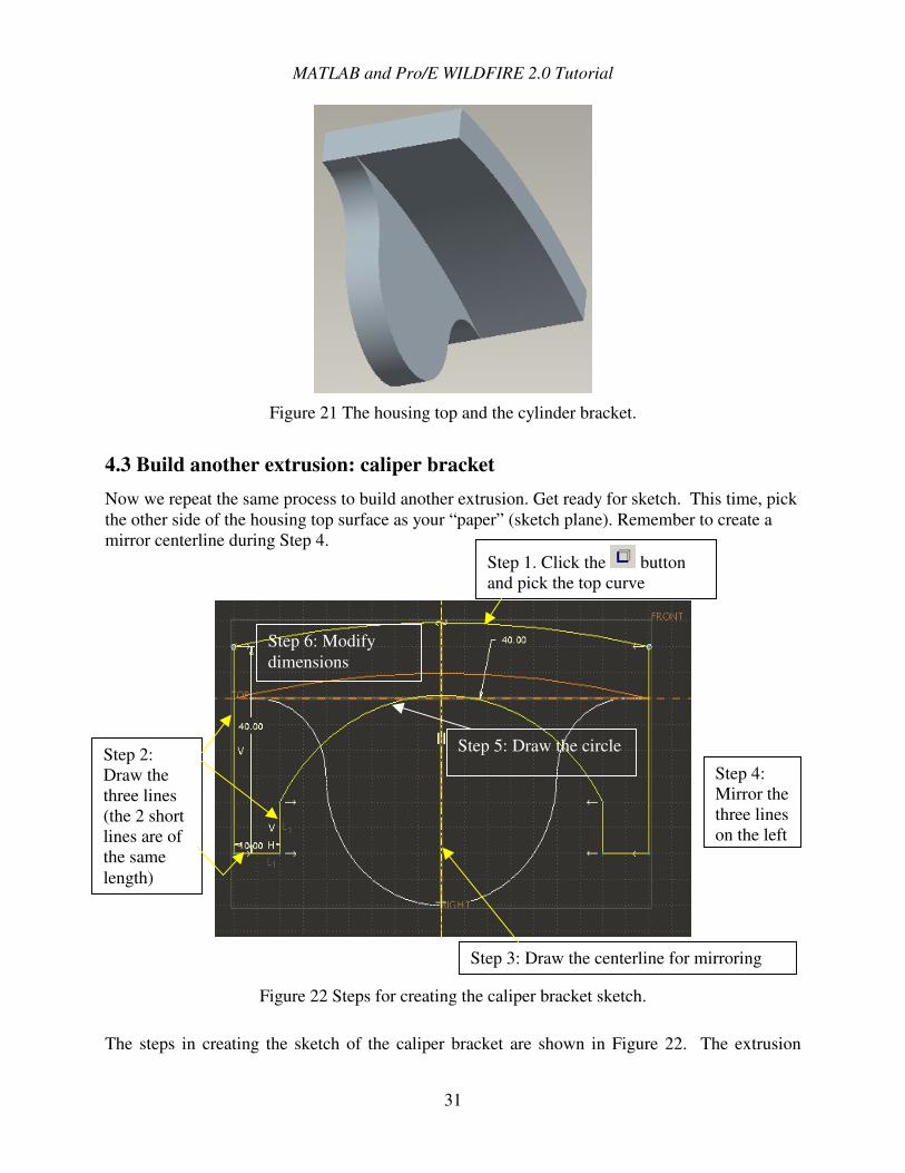
4.3 Build another extrusion: caliper bracket Now we repeat the same process to build another extrusion. Get ready for sketch. This time, pick the other side of the housing top surface as your “paper” (sketch plane). Remember to create a mirror centerline during Step 4.
Figure 22 Steps for creating the caliper bracket sketch.
The steps in creating the sketch of the caliper bracket are shown in Figure 22. The extrusion
Step 3: Draw the centerline for mirroring
Step 1. Click the button and pick the top curve
Step 2: Draw the three lines (the 2 short lines are of the same length)
Step 4: Mirror the three lines on the left
Step 5: Draw the circle
Step 6: Modify dimensions
MATLAB and Pro/E WILDFIRE 2.0 Tutorial
32
depth is [10].
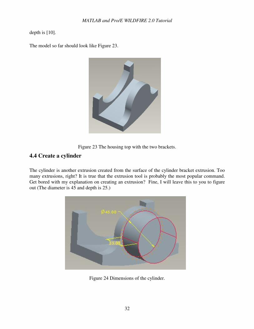
The model so far should look like Figure 23.
Figure 23 The housing top with the two brackets.
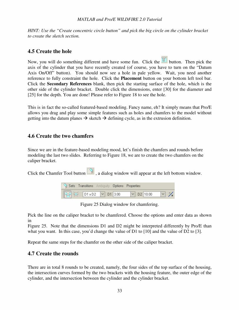
4.4 Create a cylinder
The cylinder is another extrusion created from the surface of the cylinder bracket extrusion. Too many extrusions, right? It is true that the extrusion tool is probably the most popular command. Get bored with my explanation on creating an extrusion? Fine, I will leave this to you to figure out (The diameter is 45 and depth is 25.)
Figure 24 Dimensions of the cylinder.
MATLAB and Pro/E WILDFIRE 2.0 Tutorial
33
HINT: Use the “Create concentric circle button” and pick the big circle on the cylinder bracket to create the sketch section.
4.5 Create the hole
Now, you will do something different and have some fun. Click the button. Then pick the axis of the cylinder that you have recently created (of course, you have to turn on the “Datum Axis On/Off” button). You should now see a hole in pale yellow. Wait, you need another reference to fully constraint the hole. Click the Placement button on your bottom left tool bar. Click the Secondary References blank, then pick the starting surface of the hole, which is the other side of the cylinder bracket. Double click the dimensions, enter [30] for the diameter and [25] for the depth. You are done! Please refer to Figure 18 to see the hole.
This is in fact the so-called featured-based modeling. Fancy name, eh? It simply means that Pro/E allows you drag and play some simple features such as holes and chamfers to the model without getting into the datum planes � sketch � defining cycle, as in the extrusion definition.
4.6 Create the two chamfers
Since we are in the feature-based modeling mood, let’s finish the chamfers and rounds before modeling the last two slides. Referring to Figure 18, we are to create the two chamfers on the caliper bracket.
Click the Chamfer Tool button , a dialog window will appear at the left bottom window.
Figure 25 Dialog window for chamfering.
Pick the line on the caliper bracket to be chamfered. Choose the options and enter data as shown in Figure 25. Note that the dimensions D1 and D2 might be interpreted differently by Pro/E than what you want. In this case, you’d change the value of D1 to [10] and the value of D2 to [3]. Repeat the same steps for the chamfer on the other side of the caliper bracket. 4.7 Create the rounds
There are in total 8 rounds to be created, namely, the four sides of the top surface of the housing, the intersection curves formed by the two brackets with the housing feature, the outer edge of the cylinder, and the intersection between the cylinder and the cylinder bracket.
MATLAB and Pro/E WILDFIRE 2.0 Tutorial
34
Click the Round Tool button , enter the round radius [2] in the dialog window at the left bottom window. Then pick the eight curves. These rounds should be created accordingly. Refer to Figure 18 for illustration.
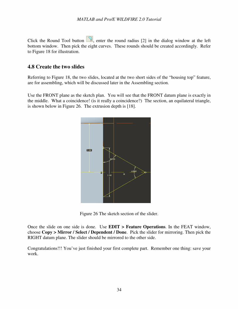
4.8 Create the two slides
Referring to Figure 18, the two slides, located at the two short sides of the “housing top” feature, are for assembling, which will be discussed later in the Assembling section.
Use the FRONT plane as the sketch plan. You will see that the FRONT datum plane is exactly in the middle. What a coincidence! (is it really a coincidence?) The section, an equilateral triangle, is shown below in Figure 26. The extrusion depth is [18].
Figure 26 The sketch section of the slider.
Once the slide on one side is done. Use EDIT > Feature Operations. In the FEAT window, choose Copy > Mirror / Select / Dependent / Done. Pick the slider for mirroring. Then pick the RIGHT datum plane. The slider should be mirrored to the other side. Congratulations!!! You’ve just finished your first complete part. Remember one thing: save your work.
MATLAB and Pro/E WILDFIRE 2.0 Tutorial
35
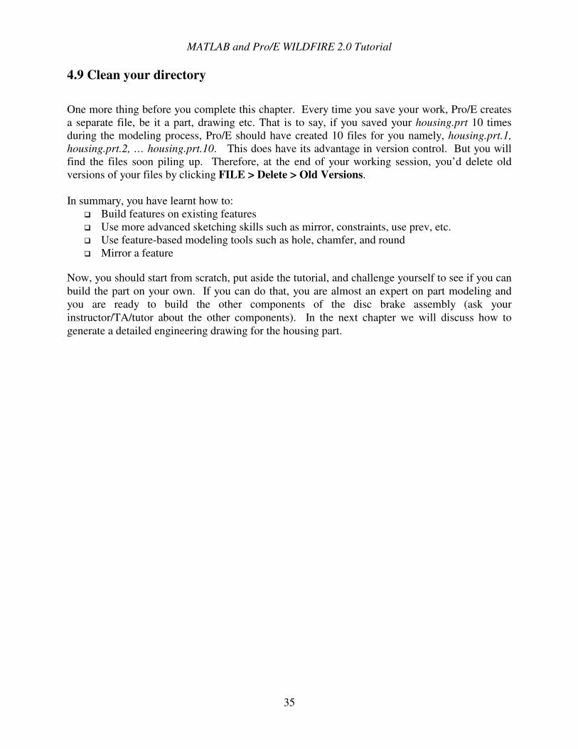
4.9 Clean your directory One more thing before you complete this chapter. Every time you save your work, Pro/E creates a separate file, be it a part, drawing etc. That is to say, if you saved your housing.prt 10 times during the modeling process, Pro/E should have created 10 files for you namely, housing.prt.1, housing.prt.2, … housing.prt.10. This does have its advantage in version control. But you will find the files soon piling up. Therefore, at the end of your working session, you’d delete old versions of your files by clicking FILE > Delete > Old Versions. In summary, you have learnt how to:
�� Build features on existing features �� Use more advanced sketching skills such as mirror, constraints, use prev, etc. �� Use feature-based modeling tools such as hole, chamfer, and round �� Mirror a feature
Now, you should start from scratch, put aside the tutorial, and challenge yourself to see if you can build the part on your own. If you can do that, you are almost an expert on part modeling and you are ready to build the other components of the disc brake assembly (ask your instructor/TA/tutor about the other components). In the next chapter we will discuss how to generate a detailed engineering drawing for the housing part.
MATLAB and Pro/E WILDFIRE 2.0 Tutorial
36
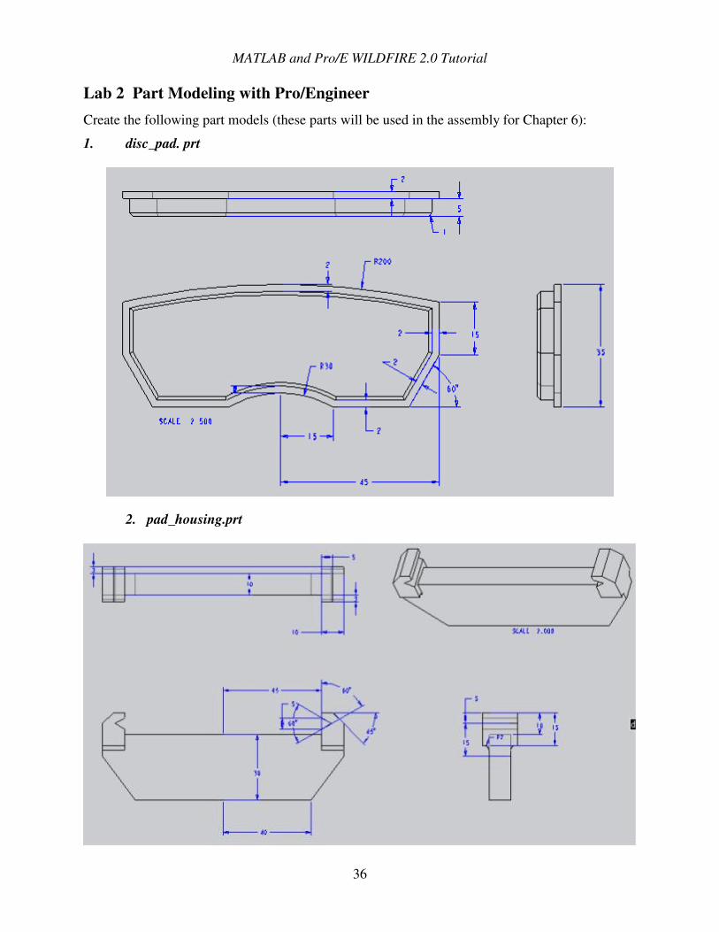
Lab 2 Part Modeling with Pro/Engineer Create the following part models (these parts will be used in the assembly for Chapter 6):
1. disc_pad. prt
2. pad_housing.prt
MATLAB and Pro/E WILDFIRE 2.0 Tutorial
37
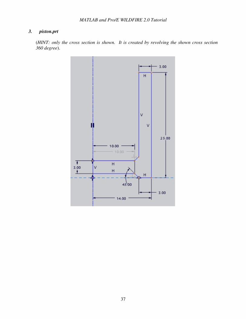
3. piston.prt (HINT: only the cross section is shown. It is created by revolving the shown cross section 360 degree).
MATLAB and Pro/E WILDFIRE 2.0 Tutorial
38
'��$�����������( ������������� ��) ����
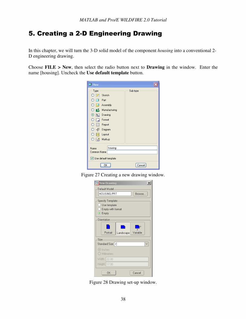
In this chapter, we will turn the 3-D solid model of the component housing into a conventional 2-D engineering drawing. Choose FILE > New, then select the radio button next to Drawing in the window. Enter the name [housing]. Uncheck the Use default template button.
Figure 27 Creating a new drawing window.
Figure 28 Drawing set-up window.
MATLAB and Pro/E WILDFIRE 2.0 Tutorial
39
A dialog window will pop-up, shown in Figure 28. Pro/E automatically brings up the part model, as long as the filename is the same. The drawing file suffix is “.drw”, a part file suffix is “.prt”, and an assembly file suffix is “.asm”. Accept all the default settings in this window. Then you will face a black box for drawing. The size setting default should probably be changed to either A4 or A3 depending on the drawing requirements.
5.1 Insert views
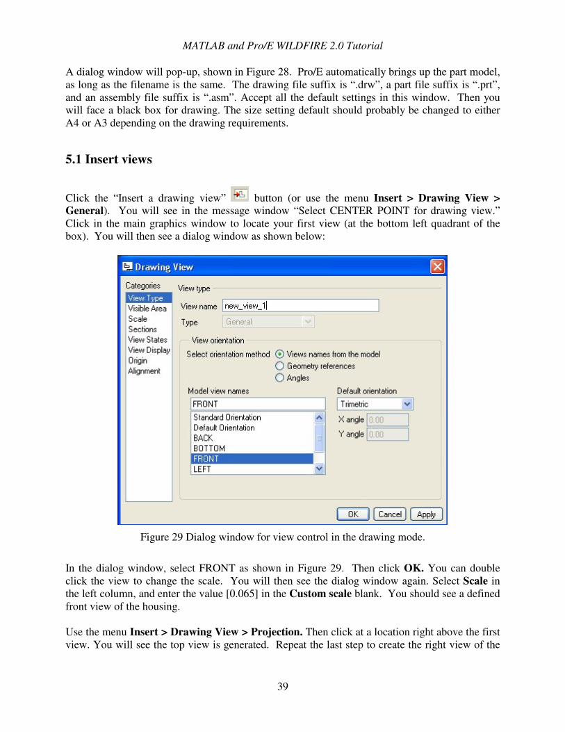
Click the “Insert a drawing view” button (or use the menu Insert > Drawing View > General). You will see in the message window “Select CENTER POINT for drawing view.” Click in the main graphics window to locate your first view (at the bottom left quadrant of the box). You will then see a dialog window as shown below:
Figure 29 Dialog window for view control in the drawing mode.
In the dialog window, select FRONT as shown in Figure 29. Then click OK. You can double click the view to change the scale. You will then see the dialog window again. Select Scale in the left column, and enter the value [0.065] in the Custom scale blank. You should see a defined front view of the housing. Use the menu Insert > Drawing View > Projection. Then click at a location right above the first view. You will see the top view is generated. Repeat the last step to create the right view of the
MATLAB and Pro/E WILDFIRE 2.0 Tutorial
40
model. (Hint: This time you need to click the front view first to specify from which view the projection is created.) You will see now your views are pretty messy with many lines and datum features. You could press all the datum view buttons and then the Redraw button to clean the drawing a little bit. Then Click TOOLS > Environment. In the last blank of the pop-up window, choose No Display for Tangent Edges. After performing a Redraw, all the tangent edges for rounds are cleaned up. The views look much better.
Last, we need to add an isometric view. This is done by clicking the again. Click the upper right quadrant for location. Since the default view of the model hides a lot of the features, the model has to be re-oriented for a better view. Please refer to Error! Reference source not found. to select Angles from the view orientation section. In the Rotation Reference blank, pick Horizontal, and enter [180] degree in the Angle value blank. Click Apply in the Orientation window, you should be able to see the isometric view. Change the scale to [0.065] in the same way as you did before on the front view. Then press the OK button.
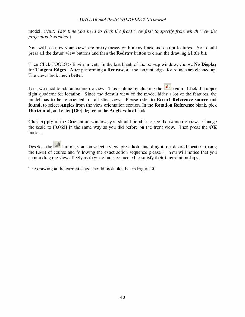
Deselect the button, you can select a view, press hold, and drag it to a desired location (using the LMB of course and following the exact action sequence please). You will notice that you cannot drag the views freely as they are inter-connected to satisfy their interrelationships. The drawing at the current stage should look like that in Figure 30.
MATLAB and Pro/E WILDFIRE 2.0 Tutorial
41
Figure 30 The drawing of Housing after the Inserting Views step.
5.2 Add dimensions
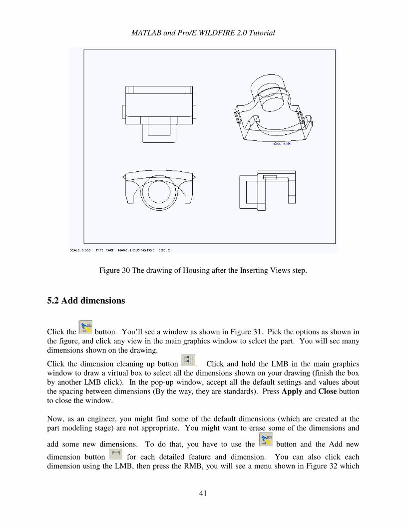
Click the button. You’ll see a window as shown in Figure 31. Pick the options as shown in the figure, and click any view in the main graphics window to select the part. You will see many dimensions shown on the drawing.
Click the dimension cleaning up button . Click and hold the LMB in the main graphics window to draw a virtual box to select all the dimensions shown on your drawing (finish the box by another LMB click). In the pop-up window, accept all the default settings and values about the spacing between dimensions (By the way, they are standards). Press Apply and Close button to close the window. Now, as an engineer, you might find some of the default dimensions (which are created at the part modeling stage) are not appropriate. You might want to erase some of the dimensions and
add some new dimensions. To do that, you have to use the button and the Add new
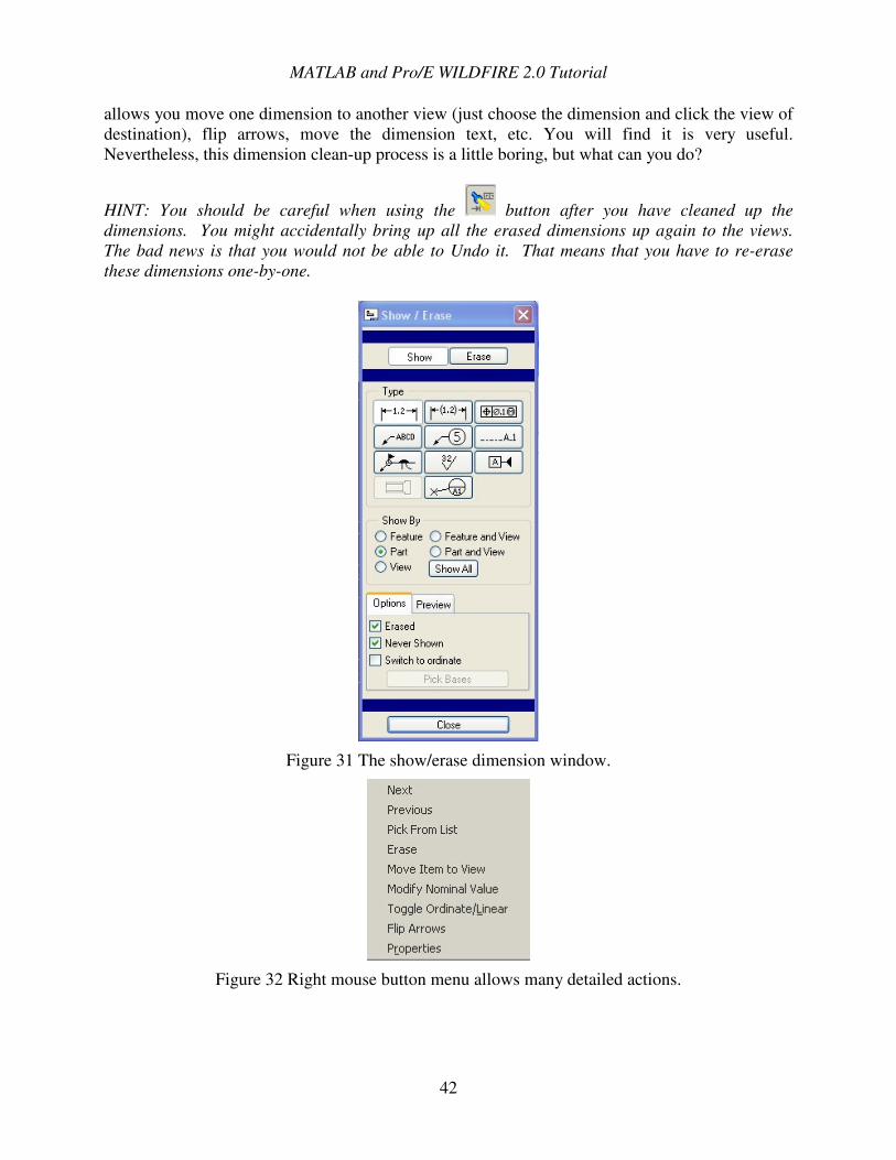
dimension button for each detailed feature and dimension. You can also click each dimension using the LMB, then press the RMB, you will see a menu shown in Figure 32 which
MATLAB and Pro/E WILDFIRE 2.0 Tutorial
42
allows you move one dimension to another view (just choose the dimension and click the view of destination), flip arrows, move the dimension text, etc. You will find it is very useful. Nevertheless, this dimension clean-up process is a little boring, but what can you do?
HINT: You should be careful when using the button after you have cleaned up the dimensions. You might accidentally bring up all the erased dimensions up again to the views. The bad news is that you would not be able to Undo it. That means that you have to re-erase these dimensions one-by-one.
Figure 31 The show/erase dimension window.
Figure 32 Right mouse button menu allows many detailed actions.
MATLAB and Pro/E WILDFIRE 2.0 Tutorial
43
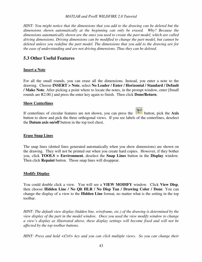
HINT: You might notice that the dimensions that you add to the drawing can be deleted but the dimensions shown automatically at the beginning can only be erased. Why? Because the dimensions automatically shown are the ones you used to create the part model, which are called driving dimensions. Driving dimensions can be modified to change the part model, but cannot be deleted unless you redefine the part model. The dimensions that you add to the drawing are for the ease of understanding and are not driving dimensions. Thus they can be deleted. 5.3 Other Useful Features
Insert a Note
For all the small rounds, you can erase all the dimensions. Instead, you enter a note to the drawing. Choose INSERT > Note, select No Leader / Enter / Horizontal / Standard / Default / Make Note. After picking a point where to locate the notes, in the prompt window, enter [Small rounds are R2.00.] and press the enter key again to finish. Then click Done/Return.
Show Centerlines
If centerlines of circular features are not shown, you can press the button, pick the Axis button to show and pick the three orthogonal views. If you see labels of the centerlines, deselect the Datum axis on/off button in the top tool chest.
Erase Snap Lines
The snap lines (dotted lines generated automatically when you show dimensions) are shown on the drawing. They will not be printed out when you create hard copies. However, if they bother you, click TOOLS > Environment, deselect the Snap Lines button in the Display window. Then click Repaint button. Those snap lines will disappear.
Modify Display
You could double click a view. You will see a VIEW MODIFY window. Click View Disp, then choose Hidden Line / No Qlt HLR / No Disp Tan / Drawing Color / Done. You can change the display of a view to the Hidden Line format, no matter what is the setting in the top toolbar.
HINT: The default view display (hidden line, wireframe, etc.) of the drawing is determined by the view display of the part in the model window. Once you used the view modify window to change a view’s display as illustrated above, these display settings will become fixed and will not be affected by the top toolbar buttons.
HINT: Press and hold <Ctrl> key and you can click multiple views. So you can change their
MATLAB and Pro/E WILDFIRE 2.0 Tutorial
44
display settings all at once.
Change the Drawing Configuration
Pro/E defines many configurations such as arrow width, arrow length, etc. By changing those configurations, you can have more freedom in creating your drawing. Now right click and hold RMB in the open space of the main graphics window (not one of the views). Select Properties, then Drawing Options. You will see a list of options. Choose Sort > Alphabetical, find the following parameters and change their settings to the values shown in Table 3.
Table 3 New values for the selected parameters.
Parameters Values drawing_text_height 0.1
draw_arrow_style FILLED draw_arrow_width 0.06 draw_arrow_length 0.16
tol_display YES After the setting change, you will see the arrows and texts are changed.
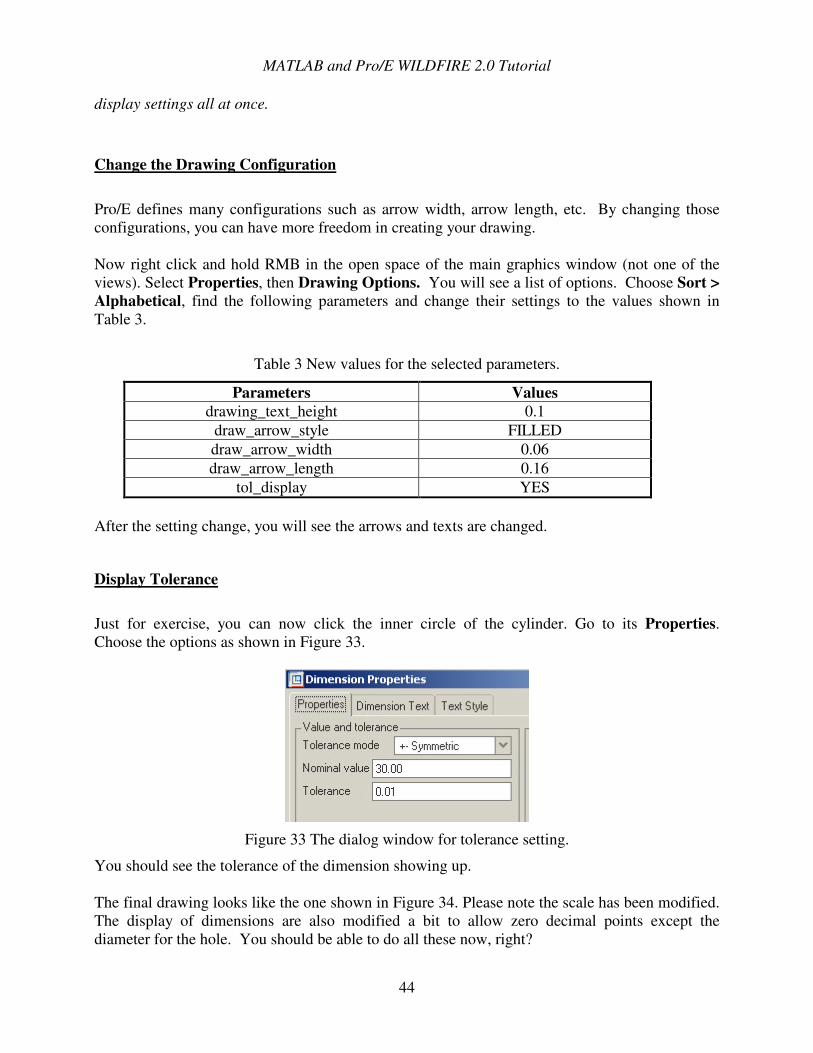
Display Tolerance
Just for exercise, you can now click the inner circle of the cylinder. Go to its Properties. Choose the options as shown in Figure 33.
Figure 33 The dialog window for tolerance setting.
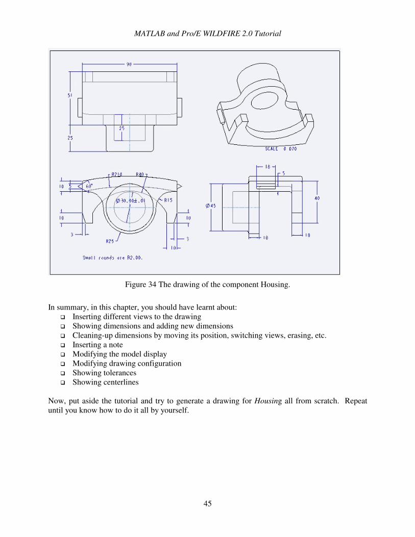
You should see the tolerance of the dimension showing up. The final drawing looks like the one shown in Figure 34. Please note the scale has been modified. The display of dimensions are also modified a bit to allow zero decimal points except the diameter for the hole. You should be able to do all these now, right?
MATLAB and Pro/E WILDFIRE 2.0 Tutorial
45
Figure 34 The drawing of the component Housing.
In summary, in this chapter, you should have learnt about:
�� Inserting different views to the drawing �� Showing dimensions and adding new dimensions �� Cleaning-up dimensions by moving its position, switching views, erasing, etc. �� Inserting a note �� Modifying the model display �� Modifying drawing configuration �� Showing tolerances �� Showing centerlines
Now, put aside the tutorial and try to generate a drawing for Housing all from scratch. Repeat until you know how to do it all by yourself.
MATLAB and Pro/E WILDFIRE 2.0 Tutorial
46
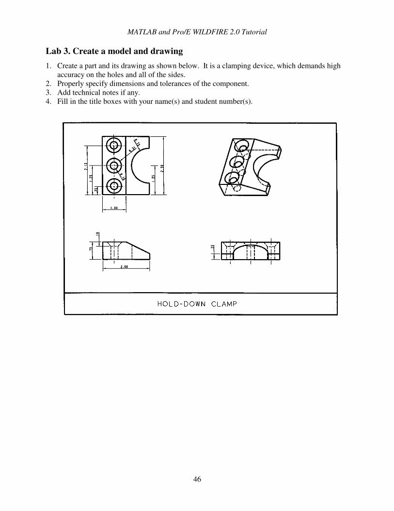
Lab 3. Create a model and drawing 1. Create a part and its drawing as shown below. It is a clamping device, which demands high
accuracy on the holes and all of the sides. 2. Properly specify dimensions and tolerances of the component. 3. Add technical notes if any. 4. Fill in the title boxes with your name(s) and student number(s).
MATLAB and Pro/E WILDFIRE 2.0 Tutorial
47
*��$������������ �+,(���,���++�% ��-�
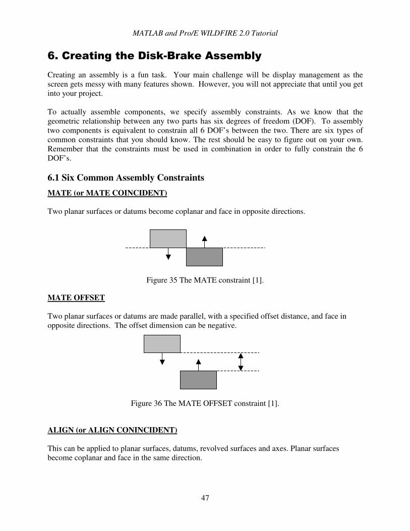
Creating an assembly is a fun task. Your main challenge will be display management as the screen gets messy with many features shown. However, you will not appreciate that until you get into your project. To actually assemble components, we specify assembly constraints. As we know that the geometric relationship between any two parts has six degrees of freedom (DOF). To assembly two components is equivalent to constrain all 6 DOF’s between the two. There are six types of common constraints that you should know. The rest should be easy to figure out on your own. Remember that the constraints must be used in combination in order to fully constrain the 6 DOF’s. 6.1 Six Common Assembly Constraints MATE (or MATE COINCIDENT) Two planar surfaces or datums become coplanar and face in opposite directions.
Figure 35 The MATE constraint [1].
MATE OFFSET Two planar surfaces or datums are made parallel, with a specified offset distance, and face in opposite directions. The offset dimension can be negative.
Figure 36 The MATE OFFSET constraint [1].
ALIGN (or ALIGN CONINCIDENT) This can be applied to planar surfaces, datums, revolved surfaces and axes. Planar surfaces become coplanar and face in the same direction.
MATLAB and Pro/E WILDFIRE 2.0 Tutorial
48
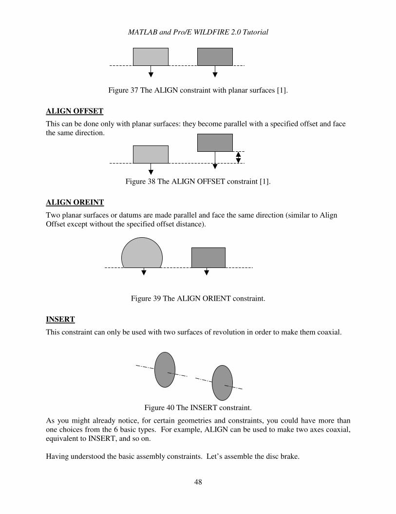
Figure 37 The ALIGN constraint with planar surfaces [1].
ALIGN OFFSET
This can be done only with planar surfaces: they become parallel with a specified offset and face the same direction.
Figure 38 The ALIGN OFFSET constraint [1].
ALIGN OREINT
Two planar surfaces or datums are made parallel and face the same direction (similar to Align Offset except without the specified offset distance).
Figure 39 The ALIGN ORIENT constraint.
INSERT
This constraint can only be used with two surfaces of revolution in order to make them coaxial.
Figure 40 The INSERT constraint.
As you might already notice, for certain geometries and constraints, you could have more than one choices from the 6 basic types. For example, ALIGN can be used to make two axes coaxial, equivalent to INSERT, and so on. Having understood the basic assembly constraints. Let’s assemble the disc brake.
MATLAB and Pro/E WILDFIRE 2.0 Tutorial
49
6.2 Build the disc-brake assembly
Use FILE > New, or click the button to launch an Assembly application. Name it [DiscBrake], and uncheck the Use default template button. In the New File Options dialog window, choose Empty. You should see an empty main graphics window with a few active buttons (comparatively). Click
the Add Component button to place the first component, which is the Housing part we created before.
Assemble the disc pad on the caliper side
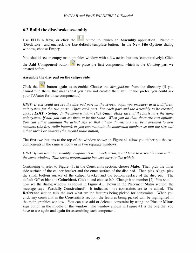
Click the button again to assemble. Choose the disc_pad.prt from the directory (if you cannot find them, that means that you have not created them yet. If you prefer, you could ask your TA/tutor for those components.) HINT: If you could not see the disc pad part on the screen, oops, you probably used a different unit system for the two parts. Open each part. For each part and the assembly to be created, choose EDIT > Setup. In the menu window, click Units. Make sure all the parts have the same unit system. If not, you can set them to be the same. When you do that, there are two options. You can either maintain the actual size so that all the dimensions will be translated to new numbers (the first radio button), or you can maintain the dimension numbers so that the size will either shrink or enlarge (the second radio button). The first two buttons at the top of the window shown in Figure 41 allow you either put the two components in the same window or in two separate windows. HINT: If you want to assembly components as a mechanism, you’d have to assemble them within the same window. This seems unreasonable but…we have to live with it. Continuing to refer to Figure 41, in the Constraints section, choose Mate. Then pick the inner side surface of the caliper bracket and the outer surface of the disc pad. Then pick Align, pick the small bottom surface of the caliper bracket and the bottom surface of the disc pad. The default Offset blank is Coincident. Click it and choose 0.0. Change it to number [2]. You should now see the dialog window as shown in Figure 41. Down in the Placement Status section, the message says “Partially Constrained”. It indicates more constraints are to be added. The Reference section tells the user what are the features being picked for constraints. When you click any constraint in the Constraints section, the features being picked will be highlighted in the main graphics window. You can also add or delete a constraint by using the Plus or Minus sign button in the middle of the window. The window shown in Figure 41 is the one that you have to use again and again for assembling each component.
MATLAB and Pro/E WILDFIRE 2.0 Tutorial
50
Figure 41 The main dialog window for assembly.
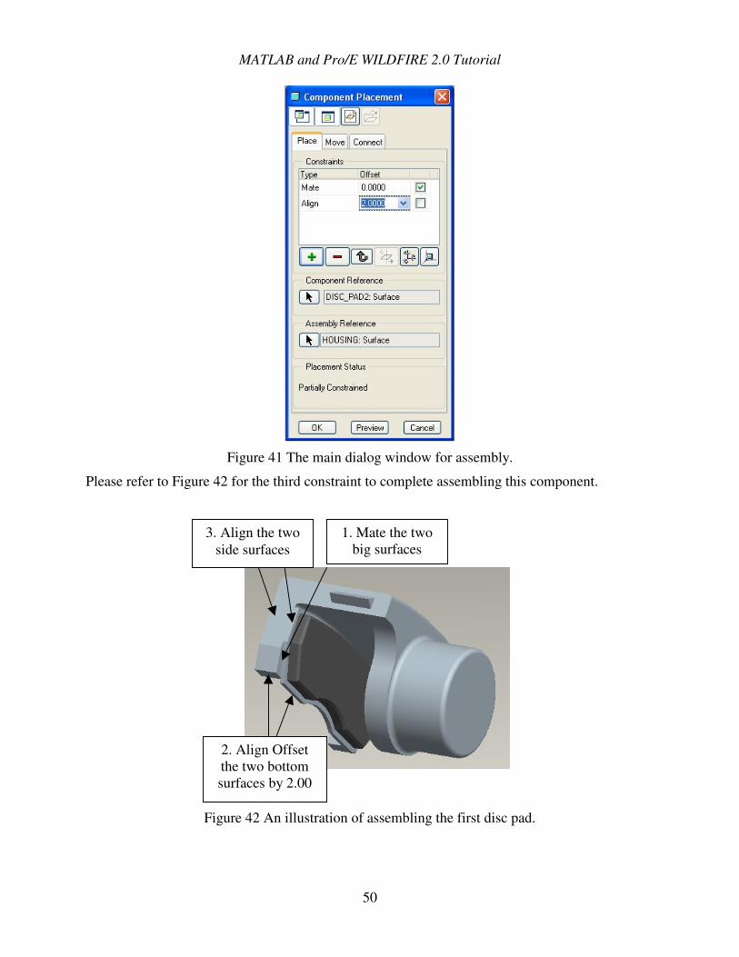
Please refer to Figure 42 for the third constraint to complete assembling this component.
Figure 42 An illustration of assembling the first disc pad.
2. Align Offset the two bottom surfaces by 2.00
3. Align the two side surfaces
1. Mate the two big surfaces
MATLAB and Pro/E WILDFIRE 2.0 Tutorial
51
Having understood the first one, the rest assembling becomes easy. So the tutorial will only give you some guidelines and leave the details to you. Are you ready?
Assemble the piston
Click and select piston.prt.
1. Use the Insert constraint and pick the outer surface of the piston and the inner surface of the hole in the part housing.
2. Use Align, pick the top surface (the open end) of the piston and the inner surface of the cylinder bracket of housing. Key in the offset number [2.0].
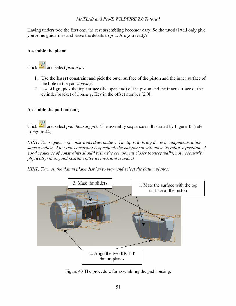
Assemble the pad housing
Click and select pad_housing.prt. The assembly sequence is illustrated by Figure 43 (refer to Figure 44). HINT: The sequence of constraints does matter. The tip is to bring the two components in the same window. After one constraint is specified, the component will move its relative position. A good sequence of constraints should bring the component closer (conceptually, not necessarily physically) to its final position after a constraint is added. HINT: Turn on the datum plane display to view and select the datum planes.
Figure 43 The procedure for assembling the pad housing.
2. Align the two RIGHT datum planes
1. Mate the surface with the top surface of the piston
3. Mate the sliders
MATLAB and Pro/E WILDFIRE 2.0 Tutorial
52
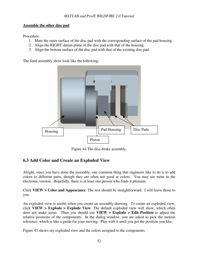
Assemble the other disc pad
Procedure:
1. Mate the outer surface of the disc pad with the corresponding surface of the pad housing. 2. Align the RIGHT datum plane of the disc pad with that of the housing. 3. Align the bottom surface of the disc pad with that of the existing disc pad.
The final assembly show look like the following:
Figure 44 The disc-brake assembly.
6.3 Add Color and Create an Exploded View Alright, since you have done the assembly, one common thing that engineers like to do is to add colors to different parts, though they are often not good at colors. You may see mine in the electronic version. Hopefully, there is at least one person who finds it pleasant. Click VIEW > Color and Appearance. The rest should be straightforward. I will leave those to you. An exploded view is useful when you create an assembly drawing. To create an exploded view, click VIEW > Explode > Explode View. The default exploded view will show, which often does not make sense. Then you should use VIEW > Explode > Edit Position to adjust the relative positions of the components. In the dialog window, you are asked to pick the motion reference, which is like a guide for your moving. Play with it until you get the position you like. Figure 45 shows my exploded view and the colors assigned to the components.
Pad Housing Disc Pads
Piston
Housing
MATLAB and Pro/E WILDFIRE 2.0 Tutorial
53
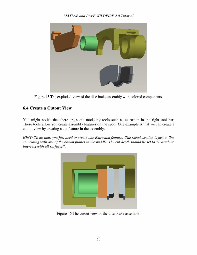
Figure 45 The exploded view of the disc brake assembly with colored components.
6.4 Create a Cutout View You might notice that there are some modeling tools such as extrusion in the right tool bar. These tools allow you create assembly features on the spot. One example is that we can create a cutout view by creating a cut feature in the assembly. HINT: To do that, you just need to create one Extrusion feature. The sketch section is just a line coinciding with one of the datum planes in the middle. The cut depth should be set to “Extrude to intersect with all surfaces”.
Figure 46 The cutout view of the disc brake assembly.

MATLAB and Pro/E WILDFIRE 2.0 Tutorial
54
In summary, you have learnt: �� basic assembly constraints �� assembling components by assembly constraints �� adding colors to components �� creating an exploded view �� creating a cutout view
Again, put aside the tutorial, do it yourself!
MATLAB and Pro/E WILDFIRE 2.0 Tutorial
55
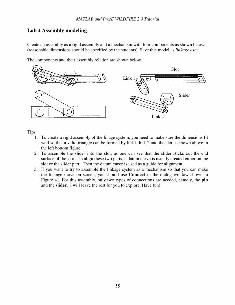
Lab 4 Assembly modeling Create an assembly as a rigid assembly and a mechanism with four components as shown below (reasonable dimensions should be specified by the students). Save this model as linkage.asm.
The components and their assembly relation are shown below.
Tips:
1. To create a rigid assembly of the linage system, you need to make sure the dimensions fit well so that a valid triangle can be formed by link1, link 2 and the slot as shown above in the left bottom figure.
2. To assemble the slider into the slot, as one can see that the slider sticks out the end surface of the slot. To align these two parts, a datum curve is usually created either on the slot or the slider part. Then the datum curve is used as a guide for alignment.
3. If you want to try to assemble the linkage system as a mechanism so that you can make the linkage move on screen, you should use Connect in the dialog window shown in Figure 41. For this assembly, only two types of connections are needed, namely, the pin and the slider. I will leave the rest for you to explore. Have fun!
Link 1
Link 2
Slider
Slot
MATLAB and Pro/E WILDFIRE 2.0 Tutorial
56
.������ ���������!���/������������-+�+0�/��+���1��-�
����-+�+0���� �+����2&��% �3������ Pro/MECHANICA is a powerful finite element analysis (FEA) package developed for design engineers. There are three main functions provided by Pro/MECHANICA.
• structural, thermal, and motion analysis; • design parameter sensitivity analysis; and • design optimization.
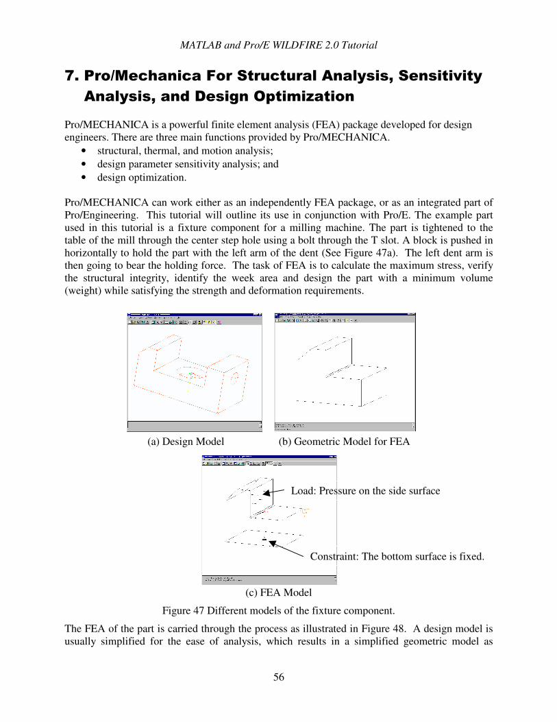
Pro/MECHANICA can work either as an independently FEA package, or as an integrated part of Pro/Engineering. This tutorial will outline its use in conjunction with Pro/E. The example part used in this tutorial is a fixture component for a milling machine. The part is tightened to the table of the mill through the center step hole using a bolt through the T slot. A block is pushed in horizontally to hold the part with the left arm of the dent (See Figure 47a). The left dent arm is then going to bear the holding force. The task of FEA is to calculate the maximum stress, verify the structural integrity, identify the week area and design the part with a minimum volume (weight) while satisfying the strength and deformation requirements.
(a) Design Model (b) Geometric Model for FEA
(c) FEA Model
Figure 47 Different models of the fixture component.
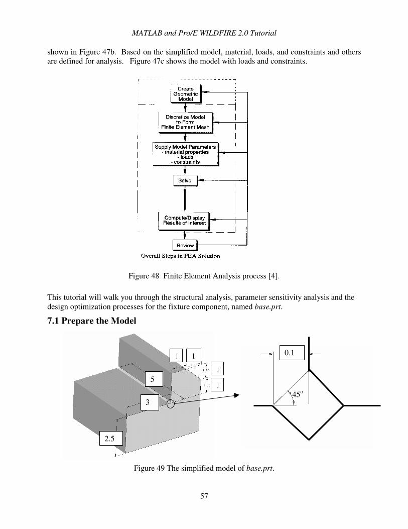
The FEA of the part is carried through the process as illustrated in Figure 48. A design model is usually simplified for the ease of analysis, which results in a simplified geometric model as
Constraint: The bottom surface is fixed.
Load: Pressure on the side surface
MATLAB and Pro/E WILDFIRE 2.0 Tutorial
57
shown in Figure 47b. Based on the simplified model, material, loads, and constraints and others are defined for analysis. Figure 47c shows the model with loads and constraints.
Figure 48 Finite Element Analysis process [4].
This tutorial will walk you through the structural analysis, parameter sensitivity analysis and the design optimization processes for the fixture component, named base.prt.
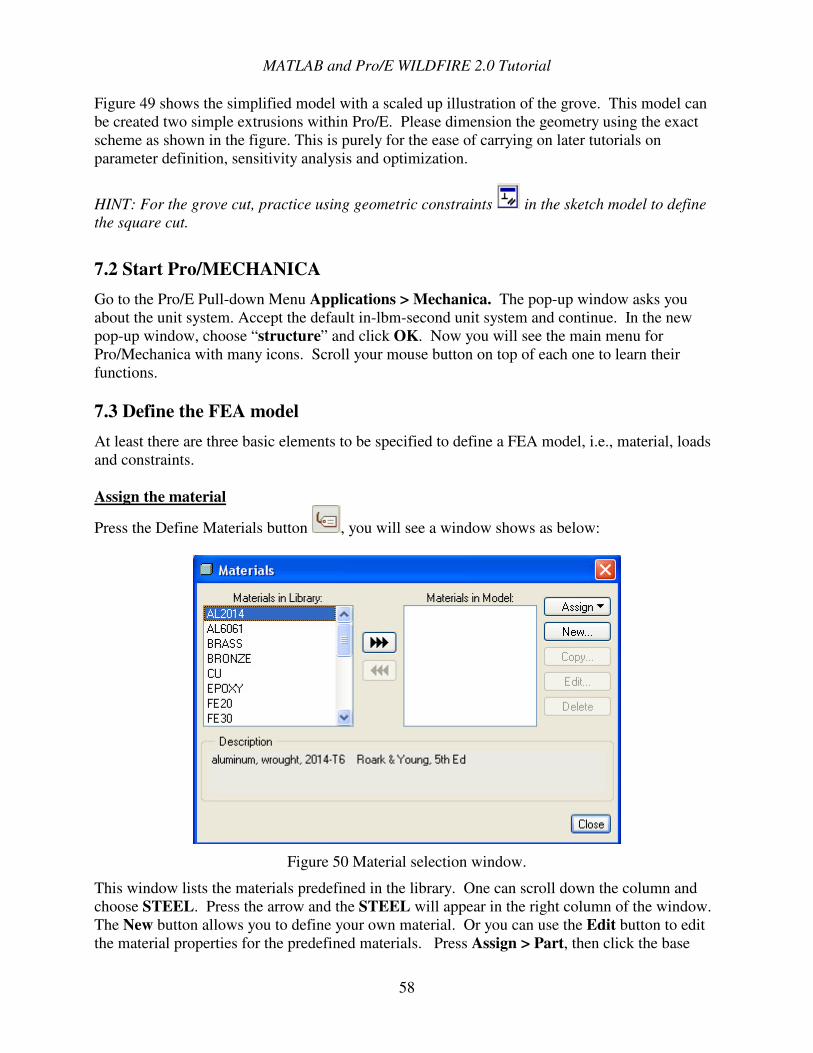
7.1 Prepare the Model
Figure 49 The simplified model of base.prt.
2.5
3
5
1 1
1
1
0.1
45o
MATLAB and Pro/E WILDFIRE 2.0 Tutorial
58
Figure 49 shows the simplified model with a scaled up illustration of the grove. This model can be created two simple extrusions within Pro/E. Please dimension the geometry using the exact scheme as shown in the figure. This is purely for the ease of carrying on later tutorials on parameter definition, sensitivity analysis and optimization.
HINT: For the grove cut, practice using geometric constraints in the sketch model to define the square cut.
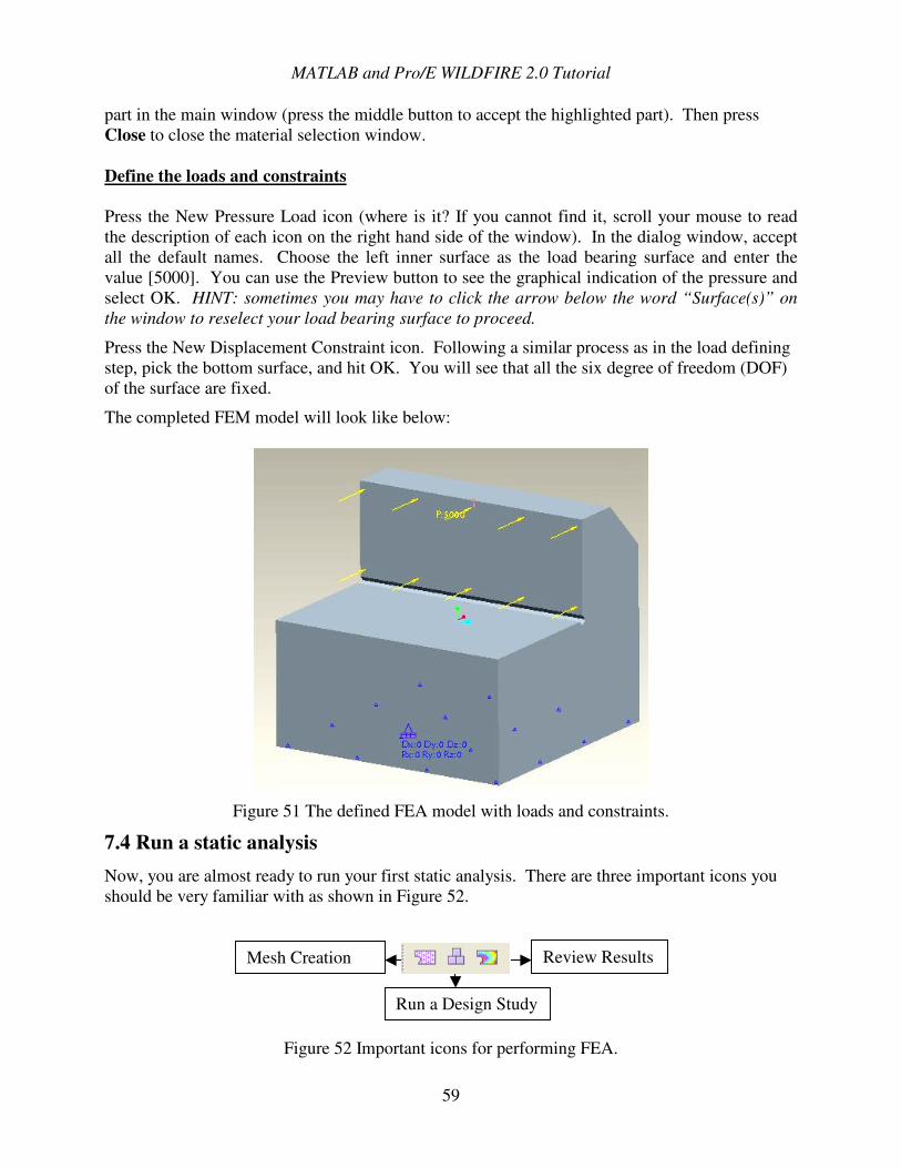
7.2 Start Pro/MECHANICA Go to the Pro/E Pull-down Menu Applications > Mechanica. The pop-up window asks you about the unit system. Accept the default in-lbm-second unit system and continue. In the new pop-up window, choose “structure” and click OK. Now you will see the main menu for Pro/Mechanica with many icons. Scroll your mouse button on top of each one to learn their functions. 7.3 Define the FEA model At least there are three basic elements to be specified to define a FEA model, i.e., material, loads and constraints. Assign the material
Press the Define Materials button , you will see a window shows as below:
Figure 50 Material selection window.
This window lists the materials predefined in the library. One can scroll down the column and choose STEEL. Press the arrow and the STEEL will appear in the right column of the window. The New button allows you to define your own material. Or you can use the Edit button to edit the material properties for the predefined materials. Press Assign > Part, then click the base
MATLAB and Pro/E WILDFIRE 2.0 Tutorial
59
part in the main window (press the middle button to accept the highlighted part). Then press Close to close the material selection window. Define the loads and constraints Press the New Pressure Load icon (where is it? If you cannot find it, scroll your mouse to read the description of each icon on the right hand side of the window). In the dialog window, accept all the default names. Choose the left inner surface as the load bearing surface and enter the value [5000]. You can use the Preview button to see the graphical indication of the pressure and select OK. HINT: sometimes you may have to click the arrow below the word “Surface(s)” on the window to reselect your load bearing surface to proceed.
Press the New Displacement Constraint icon. Following a similar process as in the load defining step, pick the bottom surface, and hit OK. You will see that all the six degree of freedom (DOF) of the surface are fixed.
The completed FEM model will look like below:
Figure 51 The defined FEA model with loads and constraints.
7.4 Run a static analysis Now, you are almost ready to run your first static analysis. There are three important icons you should be very familiar with as shown in Figure 52.
Figure 52 Important icons for performing FEA.
Mesh Creation
Run a Design Study
Review Results
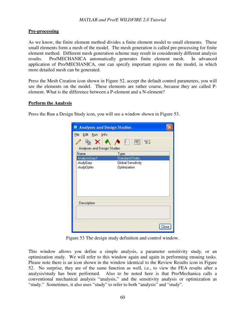
MATLAB and Pro/E WILDFIRE 2.0 Tutorial
60
Pre-processing As we know, the finite element method divides a finite element model to small elements. These small elements form a mesh of the model. The mesh generation is called pre-processing for finite element method. Different mesh generation scheme may result in considerately different analysis results. Pro/MECHANICA automatically generates finite element mesh. In advanced application of Pro/MECHANICA, one can specify important regions on the model, in which more detailed mesh can be generated. Press the Mesh Creation icon shown in Figure 52, accept the default control parameters, you will see the elements on the model. These elements are rather coarse, because they are called P-element. What is the difference between a P-element and a N-element? Perform the Analysis Press the Run a Design Study icon, you will see a window shown in Figure 53.
Figure 53 The design study definition and control window.
This window allows you define a simple analysis, a parameter sensitivity study, or an optimization study. We will refer to this window again and again in performing ensuing tasks. Please note there is an icon shown in the window identical to the Review Results icon in Figure 52. No surprise, they are of the same function as well, i.e., to view the FEA results after a analysis/study has been performed. Also to be noted here is that Pro/Mechanica calls a conventional mechanical analysis “analysis,” and the sensitivity analysis or optimization as “study.” Sometimes, it also uses “study” to refer to both “analysis” and “study”.
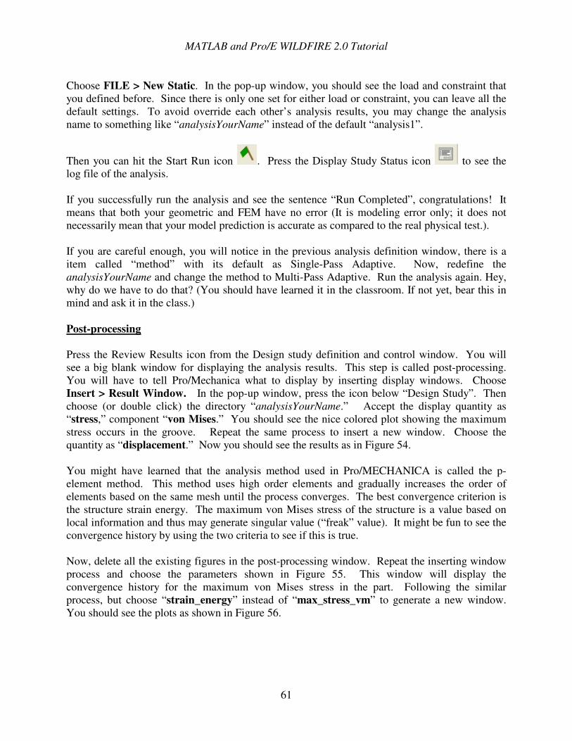
MATLAB and Pro/E WILDFIRE 2.0 Tutorial
61
Choose FILE > New Static. In the pop-up window, you should see the load and constraint that you defined before. Since there is only one set for either load or constraint, you can leave all the default settings. To avoid override each other’s analysis results, you may change the analysis name to something like “analysisYourName” instead of the default “analysis1”.
Then you can hit the Start Run icon . Press the Display Study Status icon to see the log file of the analysis. If you successfully run the analysis and see the sentence “Run Completed”, congratulations! It means that both your geometric and FEM have no error (It is modeling error only; it does not necessarily mean that your model prediction is accurate as compared to the real physical test.). If you are careful enough, you will notice in the previous analysis definition window, there is a item called “method” with its default as Single-Pass Adaptive. Now, redefine the analysisYourName and change the method to Multi-Pass Adaptive. Run the analysis again. Hey, why do we have to do that? (You should have learned it in the classroom. If not yet, bear this in mind and ask it in the class.) Post-processing Press the Review Results icon from the Design study definition and control window. You will see a big blank window for displaying the analysis results. This step is called post-processing. You will have to tell Pro/Mechanica what to display by inserting display windows. Choose Insert > Result Window. In the pop-up window, press the icon below “Design Study”. Then choose (or double click) the directory “analysisYourName.” Accept the display quantity as “stress,” component “von Mises.” You should see the nice colored plot showing the maximum stress occurs in the groove. Repeat the same process to insert a new window. Choose the quantity as “displacement.” Now you should see the results as in Figure 54. You might have learned that the analysis method used in Pro/MECHANICA is called the p-element method. This method uses high order elements and gradually increases the order of elements based on the same mesh until the process converges. The best convergence criterion is the structure strain energy. The maximum von Mises stress of the structure is a value based on local information and thus may generate singular value (“freak” value). It might be fun to see the convergence history by using the two criteria to see if this is true. Now, delete all the existing figures in the post-processing window. Repeat the inserting window process and choose the parameters shown in Figure 55. This window will display the convergence history for the maximum von Mises stress in the part. Following the similar process, but choose “strain_energy” instead of “max_stress_vm” to generate a new window. You should see the plots as shown in Figure 56.
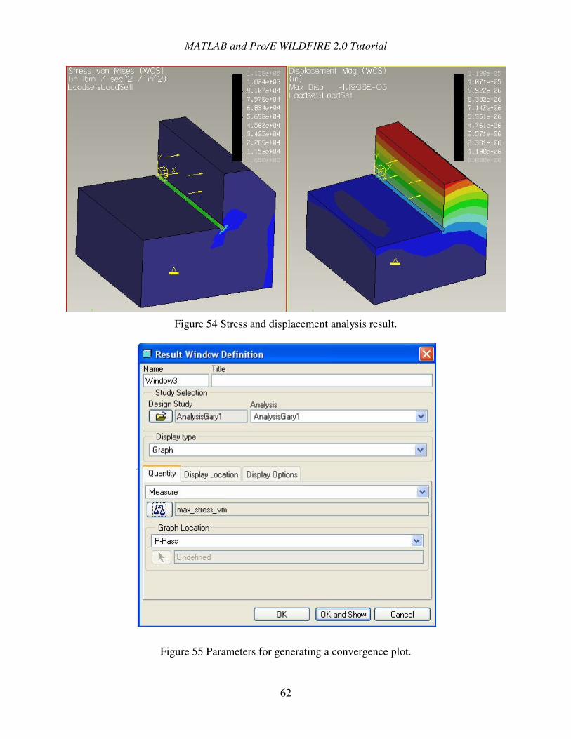
MATLAB and Pro/E WILDFIRE 2.0 Tutorial
62
Figure 54 Stress and displacement analysis result.
Figure 55 Parameters for generating a convergence plot.
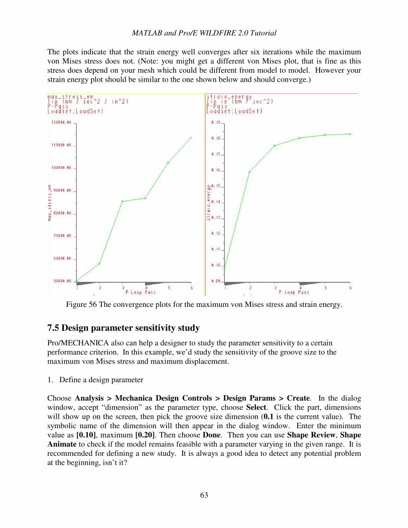
MATLAB and Pro/E WILDFIRE 2.0 Tutorial
63
The plots indicate that the strain energy well converges after six iterations while the maximum von Mises stress does not. (Note: you might get a different von Mises plot, that is fine as this stress does depend on your mesh which could be different from model to model. However your strain energy plot should be similar to the one shown below and should converge.)
Figure 56 The convergence plots for the maximum von Mises stress and strain energy.
7.5 Design parameter sensitivity study Pro/MECHANICA also can help a designer to study the parameter sensitivity to a certain performance criterion. In this example, we’d study the sensitivity of the groove size to the maximum von Mises stress and maximum displacement. 1. Define a design parameter
Choose Analysis > Mechanica Design Controls > Design Params > Create. In the dialog window, accept “dimension” as the parameter type, choose Select. Click the part, dimensions will show up on the screen, then pick the groove size dimension (0.1 is the current value). The symbolic name of the dimension will then appear in the dialog window. Enter the minimum value as [0.10], maximum [0.20]. Then choose Done. Then you can use Shape Review, Shape Animate to check if the model remains feasible with a parameter varying in the given range. It is recommended for defining a new study. It is always a good idea to detect any potential problem at the beginning, isn’t it?
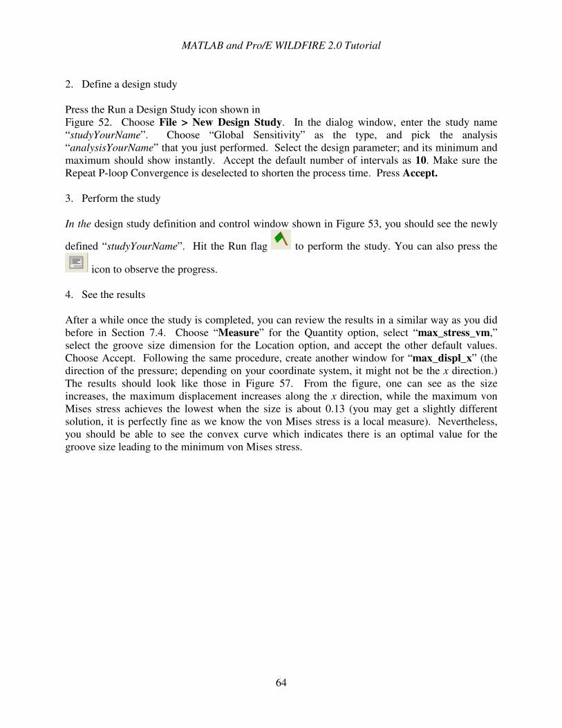
MATLAB and Pro/E WILDFIRE 2.0 Tutorial
64
2. Define a design study Press the Run a Design Study icon shown in Figure 52. Choose File > New Design Study. In the dialog window, enter the study name “studyYourName”. Choose “Global Sensitivity” as the type, and pick the analysis “analysisYourName” that you just performed. Select the design parameter; and its minimum and maximum should show instantly. Accept the default number of intervals as 10. Make sure the Repeat P-loop Convergence is deselected to shorten the process time. Press Accept. 3. Perform the study In the design study definition and control window shown in Figure 53, you should see the newly
defined “studyYourName”. Hit the Run flag to perform the study. You can also press the
icon to observe the progress. 4. See the results After a while once the study is completed, you can review the results in a similar way as you did before in Section 7.4. Choose “Measure” for the Quantity option, select “max_stress_vm,” select the groove size dimension for the Location option, and accept the other default values. Choose Accept. Following the same procedure, create another window for “max_displ_x” (the direction of the pressure; depending on your coordinate system, it might not be the x direction.) The results should look like those in Figure 57. From the figure, one can see as the size increases, the maximum displacement increases along the x direction, while the maximum von Mises stress achieves the lowest when the size is about 0.13 (you may get a slightly different solution, it is perfectly fine as we know the von Mises stress is a local measure). Nevertheless, you should be able to see the convex curve which indicates there is an optimal value for the groove size leading to the minimum von Mises stress.
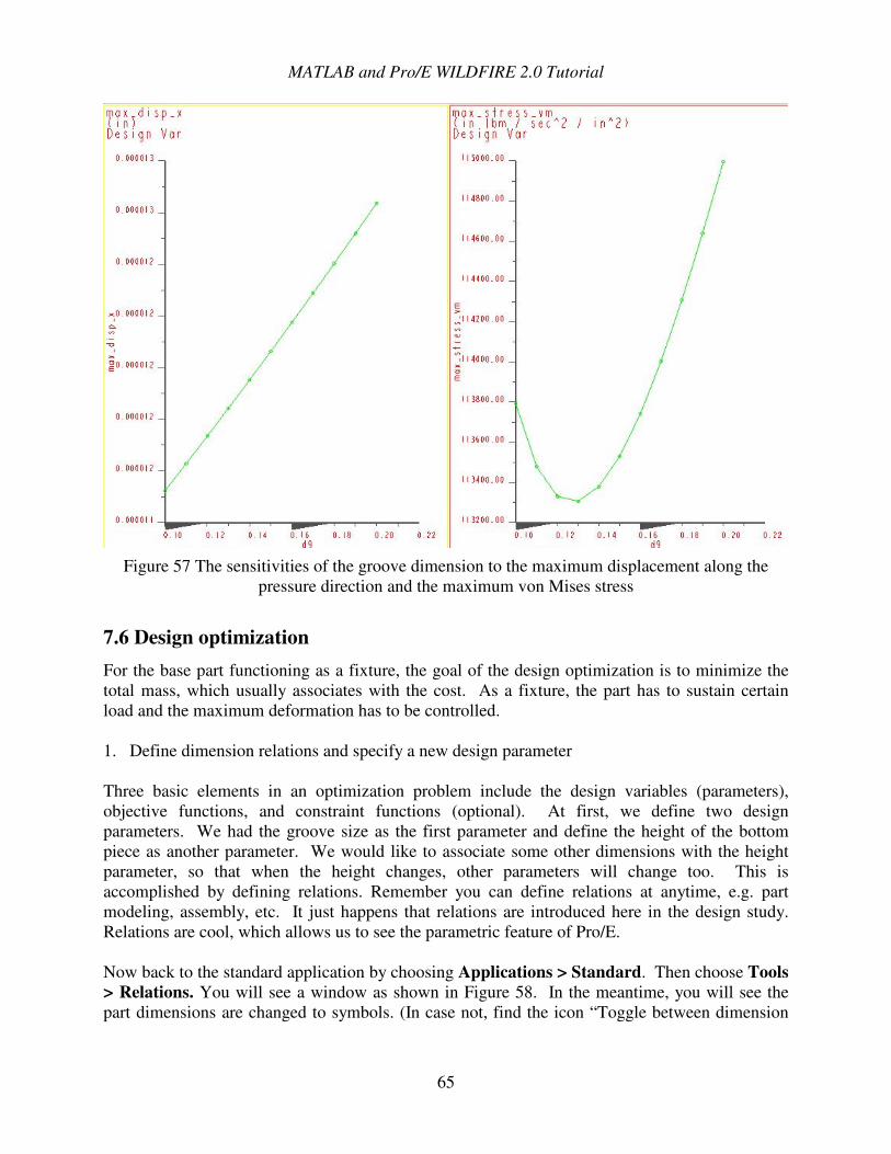
MATLAB and Pro/E WILDFIRE 2.0 Tutorial
65
Figure 57 The sensitivities of the groove dimension to the maximum displacement along the
pressure direction and the maximum von Mises stress
7.6 Design optimization For the base part functioning as a fixture, the goal of the design optimization is to minimize the total mass, which usually associates with the cost. As a fixture, the part has to sustain certain load and the maximum deformation has to be controlled. 1. Define dimension relations and specify a new design parameter Three basic elements in an optimization problem include the design variables (parameters), objective functions, and constraint functions (optional). At first, we define two design parameters. We had the groove size as the first parameter and define the height of the bottom piece as another parameter. We would like to associate some other dimensions with the height parameter, so that when the height changes, other parameters will change too. This is accomplished by defining relations. Remember you can define relations at anytime, e.g. part modeling, assembly, etc. It just happens that relations are introduced here in the design study. Relations are cool, which allows us to see the parametric feature of Pro/E. Now back to the standard application by choosing Applications > Standard. Then choose Tools > Relations. You will see a window as shown in Figure 58. In the meantime, you will see the part dimensions are changed to symbols. (In case not, find the icon “Toggle between dimension
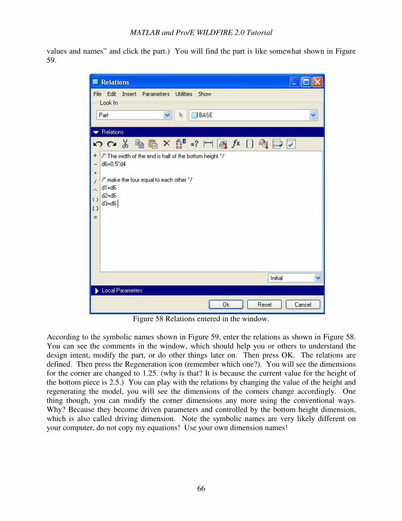
MATLAB and Pro/E WILDFIRE 2.0 Tutorial
66
values and names” and click the part.) You will find the part is like somewhat shown in Figure 59.
Figure 58 Relations entered in the window.
According to the symbolic names shown in Figure 59, enter the relations as shown in Figure 58. You can see the comments in the window, which should help you or others to understand the design intent, modify the part, or do other things later on. Then press OK. The relations are defined. Then press the Regeneration icon (remember which one?). You will see the dimensions for the corner are changed to 1.25. (why is that? It is because the current value for the height of the bottom piece is 2.5.) You can play with the relations by changing the value of the height and regenerating the model, you will see the dimensions of the corners change accordingly. One thing though, you can modify the corner dimensions any more using the conventional ways. Why? Because they become driven parameters and controlled by the bottom height dimension, which is also called driving dimension. Note the symbolic names are very likely different on your computer, do not copy my equations! Use your own dimension names!
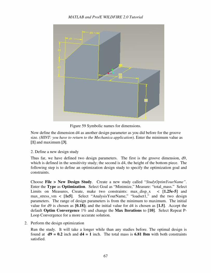
MATLAB and Pro/E WILDFIRE 2.0 Tutorial
67
Figure 59 Symbolic names for dimensions.
Now define the dimension d4 as another design parameter as you did before for the groove size. (HINT: you have to return to the Mechanica application). Enter the minimum value as [1] and maximum [3]. 2. Define a new design study
Thus far, we have defined two design parameters. The first is the groove dimension, d9, which is defined in the sensitivity study; the second is d4, the height of the bottom piece. The following step is to define an optimization design study to specify the optimization goal and constraints. Choose File > New Design Study. Create a new study called “StudyOptimYourName”. Enter the Type as Optimization. Select Goal as “Minimize,” Measure: “total_mass.” Select Limits on Measures, Create, make two constraints: max_disp_x < [1.25e-5] and max_stress_vm < [1e5]. Select “AnalysisYourName,” “loadset1,” and the two design parameters. The range of design parameters is from the minimum to maximum. The initial value for d9 is chosen as [0.18]; and the initial value for d4 is chosen as [1.5]. Accept the default Optim Convergence 1% and change the Max Iterations to [10]. Select Repeat P-Loop Convergence for a more accurate solution.
2. Perform the design optimization
Run the study. It will take a longer while than any studies before. The optimal design is found at d9 = 0.2 inch and d4 = 1 inch. The total mass is 6.81 lbm with both constraints satisfied.
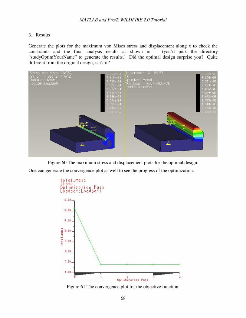
MATLAB and Pro/E WILDFIRE 2.0 Tutorial
68
3. Results Generate the plots for the maximum von Mises stress and displacement along x to check the constraints and the final analysis results as shown in (you’d pick the directory “studyOptimYourName” to generate the results.) Did the optimal design surprise you? Quite different from the original design, isn’t it?
Figure 60 The maximum stress and displacement plots for the optimal design.
One can generate the convergence plot as well to see the progress of the optimization.
Figure 61 The convergence plot for the objective function.

MATLAB and Pro/E WILDFIRE 2.0 Tutorial
69
The convergence plot Figure 61 tells us the history of optimization. To generate the plot, just create a graph plot, using the total_mass as the Measure and accept the other defaults. As one can see, the total mass converges to the minimum as the last iterations.

MATLAB and Pro/E WILDFIRE 2.0 Tutorial
70
Lab 5 FEA Practice Follow the tutorials in this chapter and show the results to TAs for all the necessary results.
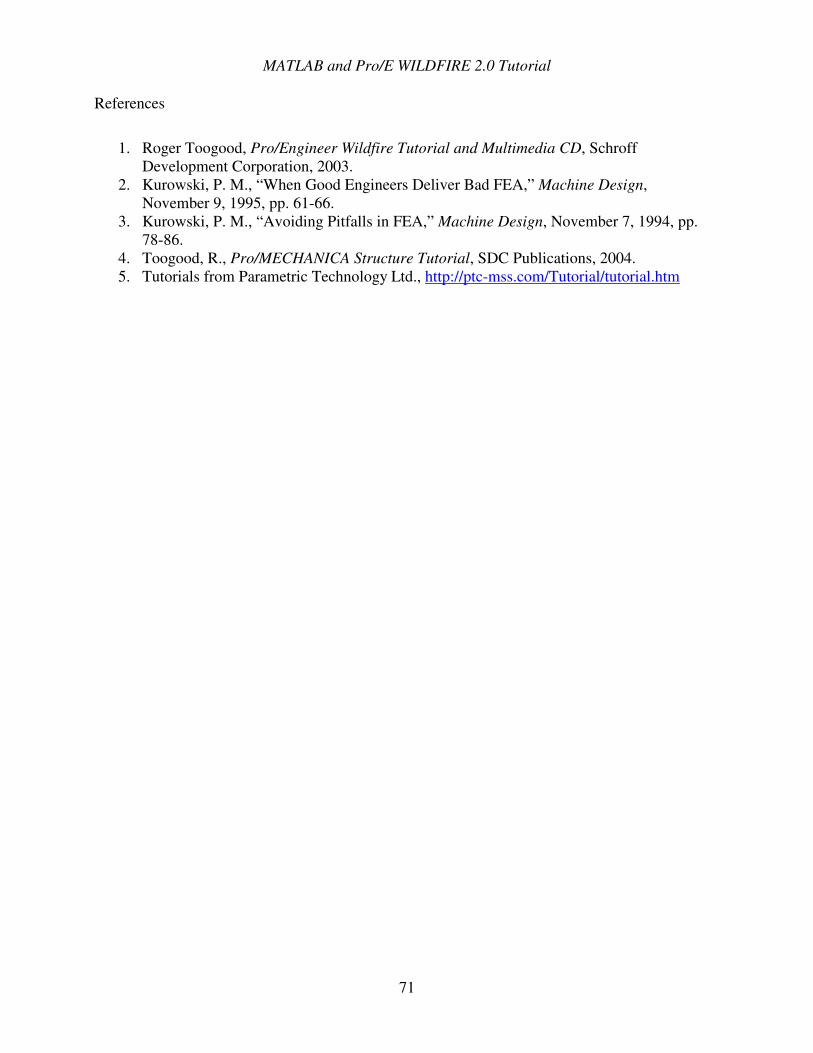
MATLAB and Pro/E WILDFIRE 2.0 Tutorial
71
References
1. Roger Toogood, Pro/Engineer Wildfire Tutorial and Multimedia CD, Schroff Development Corporation, 2003.
2. Kurowski, P. M., “When Good Engineers Deliver Bad FEA,” Machine Design, November 9, 1995, pp. 61-66.
3. Kurowski, P. M., “Avoiding Pitfalls in FEA,” Machine Design, November 7, 1994, pp. 78-86.
4. Toogood, R., Pro/MECHANICA Structure Tutorial, SDC Publications, 2004. 5. Tutorials from Parametric Technology Ltd., http://ptc-mss.com/Tutorial/tutorial.htm
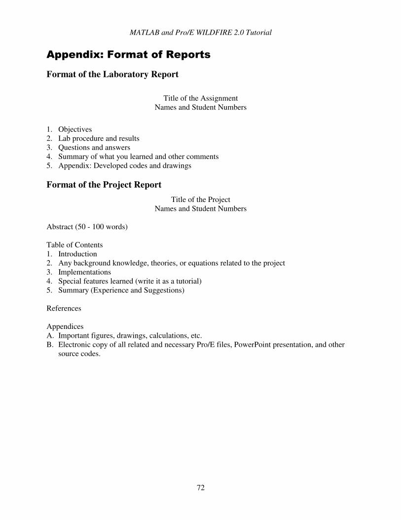
MATLAB and Pro/E WILDFIRE 2.0 Tutorial
72
�&&���45�!��% ������"�&���+�
Format of the Laboratory Report
Title of the Assignment Names and Student Numbers
1. Objectives 2. Lab procedure and results 3. Questions and answers 4. Summary of what you learned and other comments 5. Appendix: Developed codes and drawings Format of the Project Report
Title of the Project Names and Student Numbers
Abstract (50 - 100 words) Table of Contents 1. Introduction 2. Any background knowledge, theories, or equations related to the project 3. Implementations 4. Special features learned (write it as a tutorial) 5. Summary (Experience and Suggestions) References Appendices A. Important figures, drawings, calculations, etc. B. Electronic copy of all related and necessary Pro/E files, PowerPoint presentation, and other
source codes.


![MATLAB Tutorials - MIT...16.62x MATLAB Tutorials Linear Regression Multiple linear regression >> [B, Bint, R, Rint, stats] = regress(y, X)B: vector of regression coefficients Bint:](https://img.pdfslide.net/doc/110x75/606cf68397efb217626327d9/matlab-tutorials-mit-1662x-matlab-tutorials-linear-regression-multiple-linear.jpg)