Tutorials on DAMASK Crystal Plasticity Software

Based on lecture notes of Philip Eisenlohr (MSU) Prepared by Praveen Kumar (IISc)

Tutorial 1: Uniaxial tension type loading on an isotropic material (no specific slip system) Tutorial 2: Uniaxial tension type loading on a crystalline material (specific slip systems, etc.) Tutorial 3: Uniaxial compression type loading on a 2-phase alloy

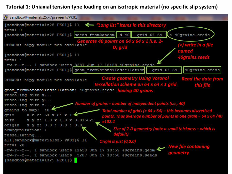
“Long list” items in this directory

Generate 40 points on 64 x 64 x 1 (i.e. 2-D) grid (>) write in a file

named 40grains.seeds

Create geometry Using Voronoi Tessellation scheme on 64 x 64 x 1 grid

having 40 grains

Read the data from this file

Number of grains = number of independent points (i.e., 40)

Total number of grids (= 64 x 64) – this becomes discretised points. Thus average number of points in one grain = 64 x 64 /40 =102.4

Size of 2-D geometry (note a small thickness – which is default)

Origin is just (0,0,0) New file containing geometry

Tutorial 1: Uniaxial tension type loading on an isotropic material (no specific slip system)

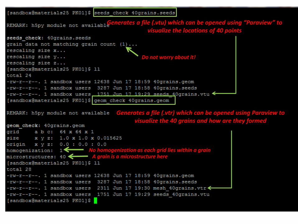
Generates a file (.vtu) which can be opened using “Paraview” to visualize the locations of 40 points

Do not worry about it!

Generates a file (.vtr) which can be opened using Paraview to visualize the 40 grains and how are they formed

A grain is a microstructure here No homogenization as each grid lies within a grain

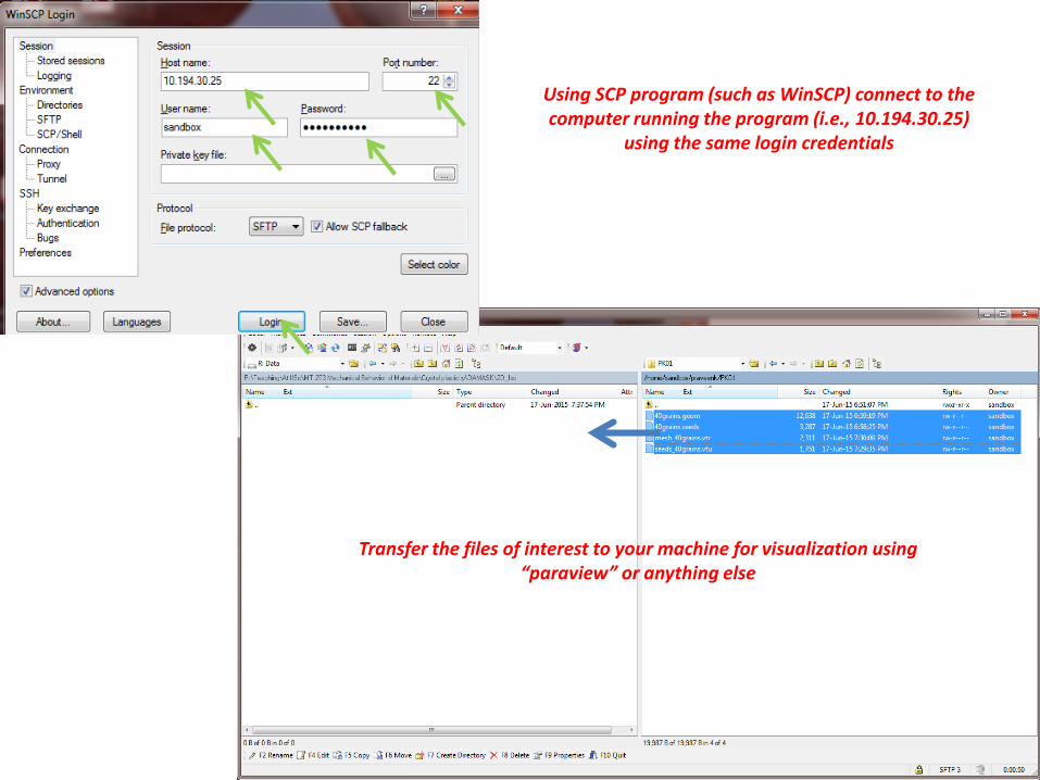
Transfer the files of interest to your machine for visualization using “paraview” or anything else

Using SCP program (such as WinSCP) connect to the computer running the program (i.e., 10.194.30.25)

using the same login credentials

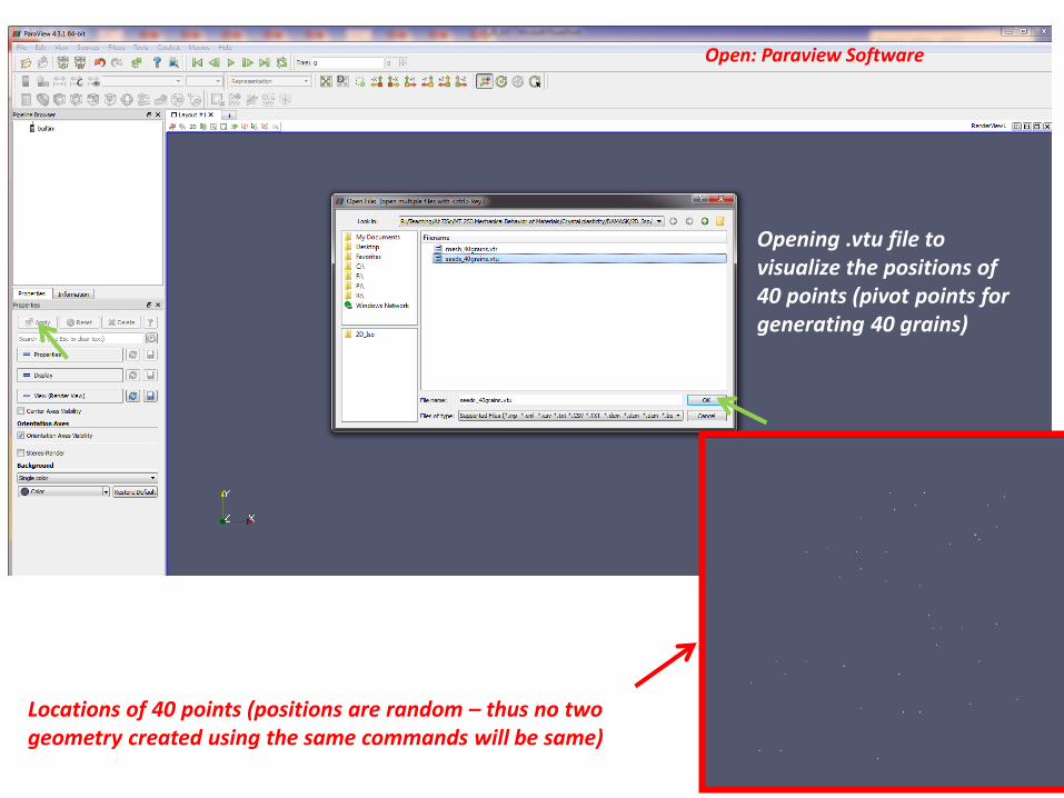
Opening .vtu file to visualize the positions of 40 points (pivot points for generating 40 grains)

Locations of 40 points (positions are random – thus no two geometry created using the same commands will be same)

Open: Paraview Software

I

II

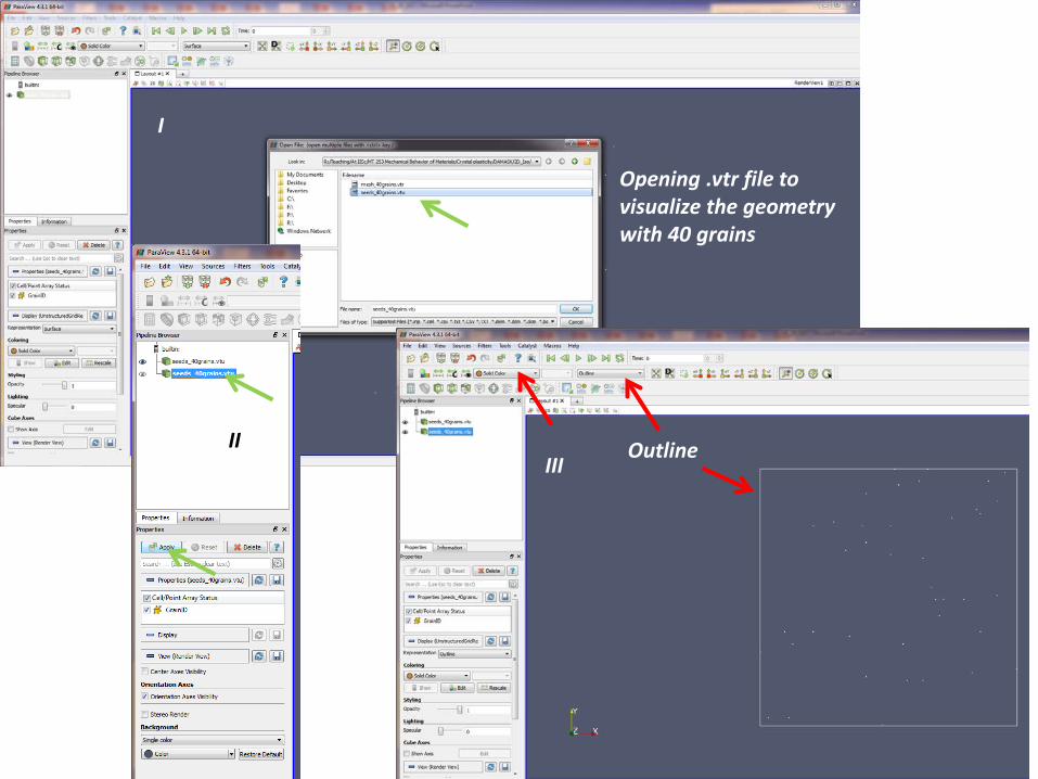
Opening .vtr file to visualize the geometry with 40 grains

Outline III

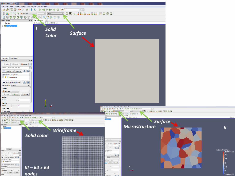
I Surface

II Surface

Solid Color

Microstructure

III – 64 x 64 nodes

Solid color Wireframe

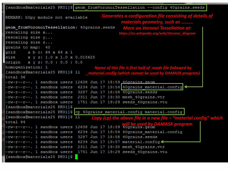
Generates a configuration file consisting of details of materials geometry, such as ………. More on Voronoi Tessellation at:

https://en.wikipedia.org/wiki/Voronoi_diagram

Copy (cp) the above file in a new file – “material.config” which will be used by DAMASK program

Name of this file is first half of .seeds file followed by _material.config (which cannot be used by DAMASK program)

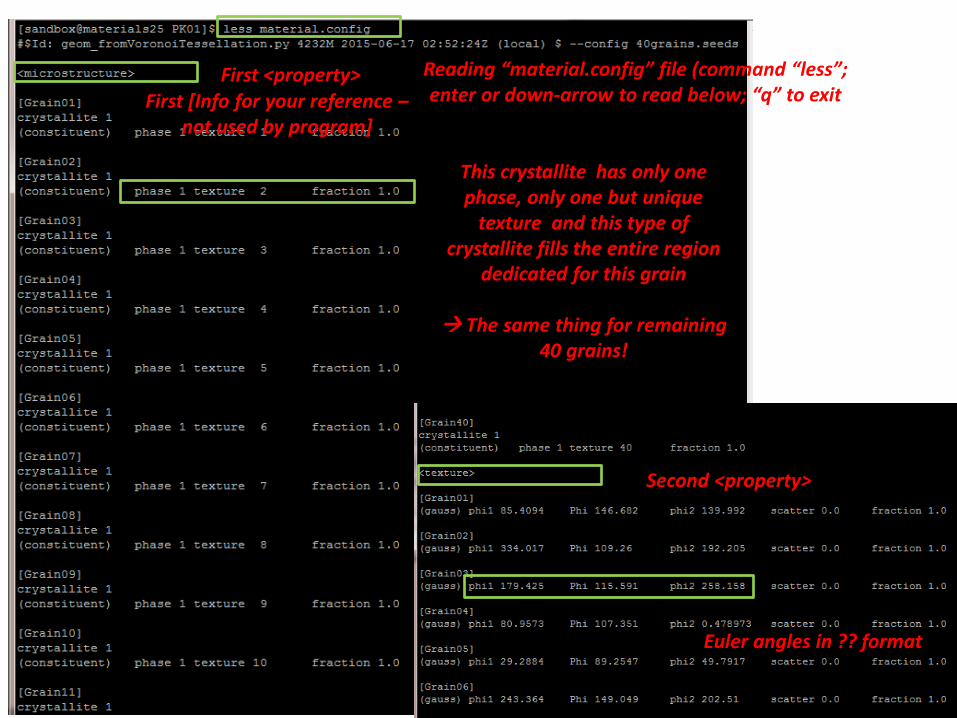
Reading “material.config” file (command “less”; enter or down-arrow to read below; “q” to exit

First <property>

This crystallite has only one phase, only one but unique

texture and this type of crystallite fills the entire region

dedicated for this grain

The same thing for remaining 40 grains!

Second <property>

Euler angles in ?? format

First [Info for your reference – not used by program]

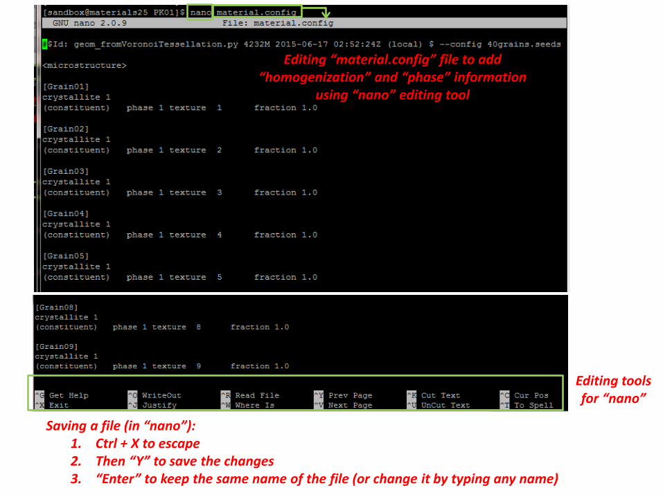
Editing “material.config” file to add “homogenization” and “phase” information

using “nano” editing tool

Editing tools for “nano”

Saving a file (in “nano”): 1. Ctrl + X to escape 2. Then “Y” to save the changes 3. “Enter” to keep the same name of the file (or change it by typing any name)

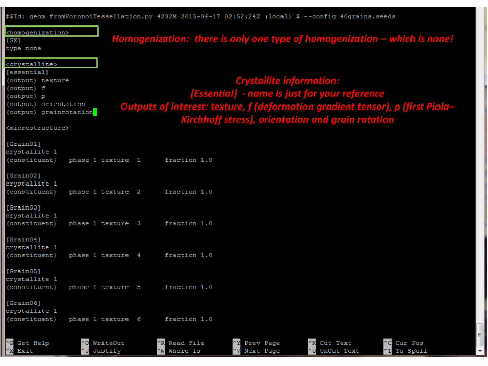
Homogenization: there is only one type of homogenization – which is none!

Crystallite information: [Essential] - name is just for your reference

Outputs of interest: texture, f (deformation gradient tensor), p (first Piola–Kirchhoff stress), orientation and grain rotation

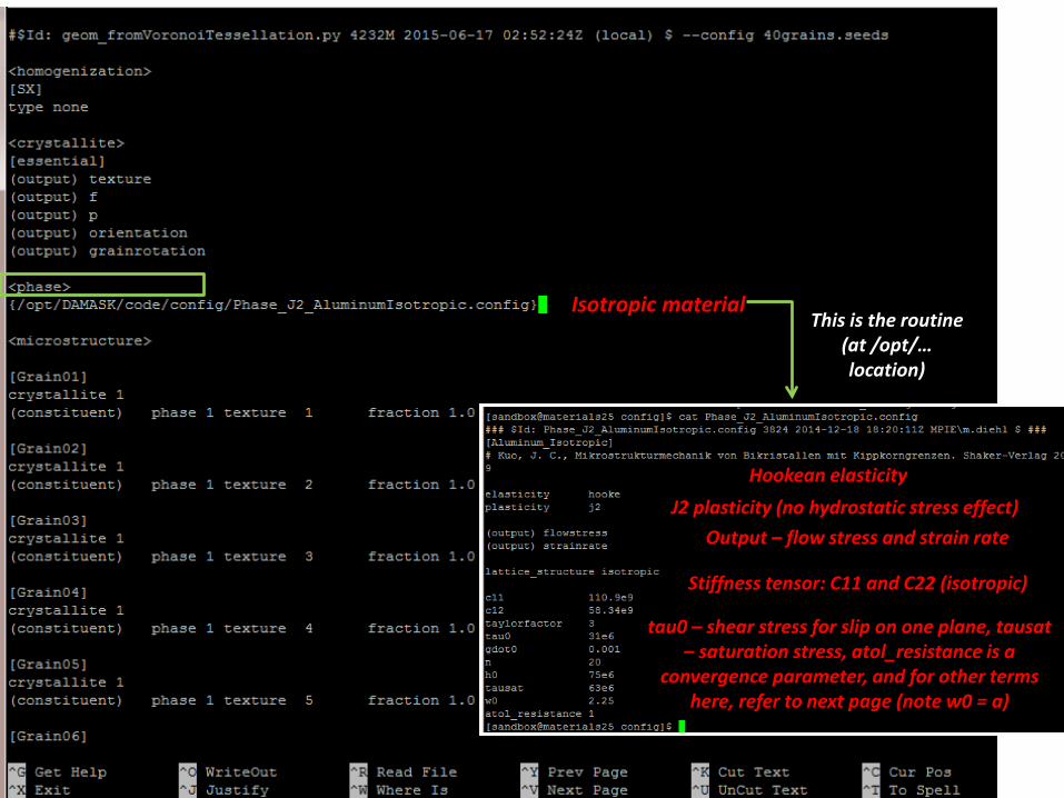
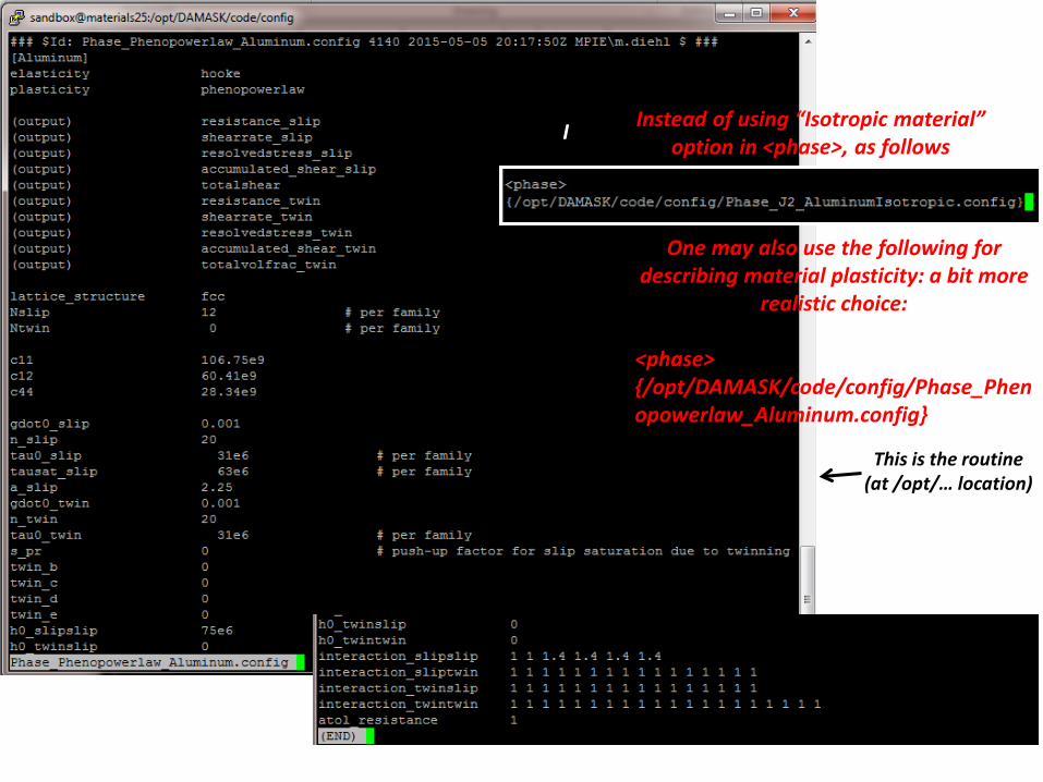
Isotropic material

Hookean elasticity J2 plasticity (no hydrostatic stress effect)

Output – flow stress and strain rate

Stiffness tensor: C11 and C22 (isotropic)

tau0 – shear stress for slip on one plane, tausat – saturation stress, atol_resistance is a

convergence parameter, and for other terms here, refer to next page (note w0 = a)

This is the routine (at /opt/… location)

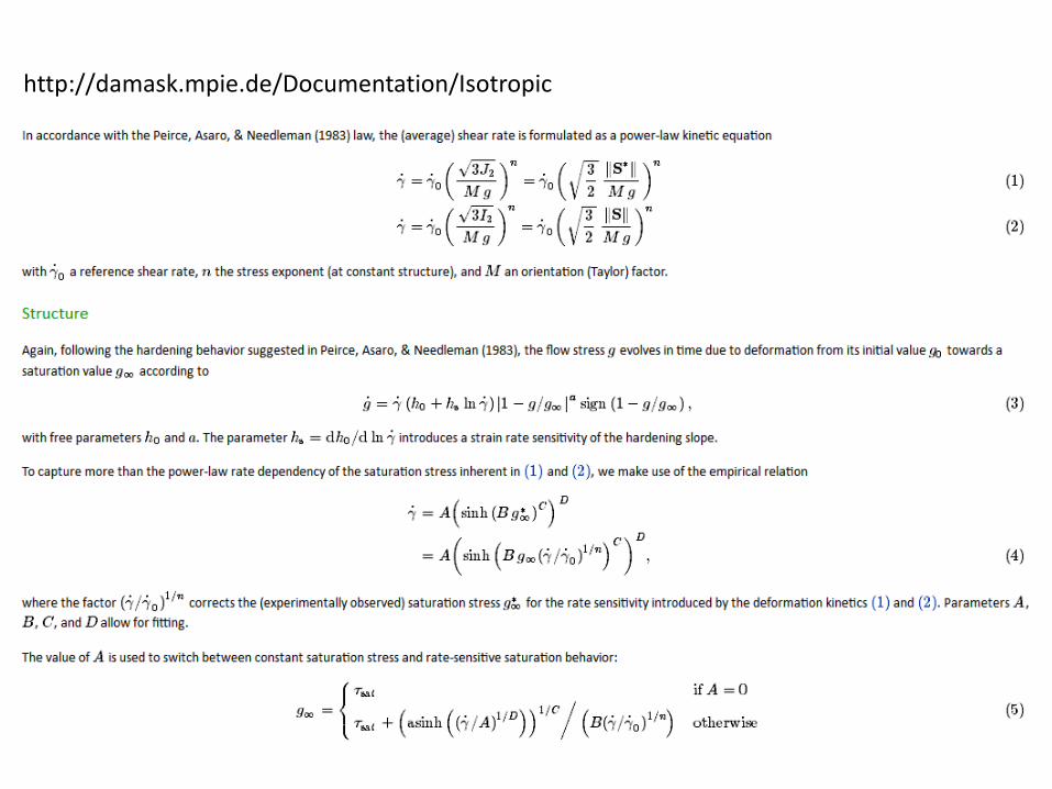
http://damask.mpie.de/Documentation/Isotropic

I

II

Instead of using “Isotropic material” option in <phase>, as follows

One may also use the following for describing material plasticity: a bit more

realistic choice:

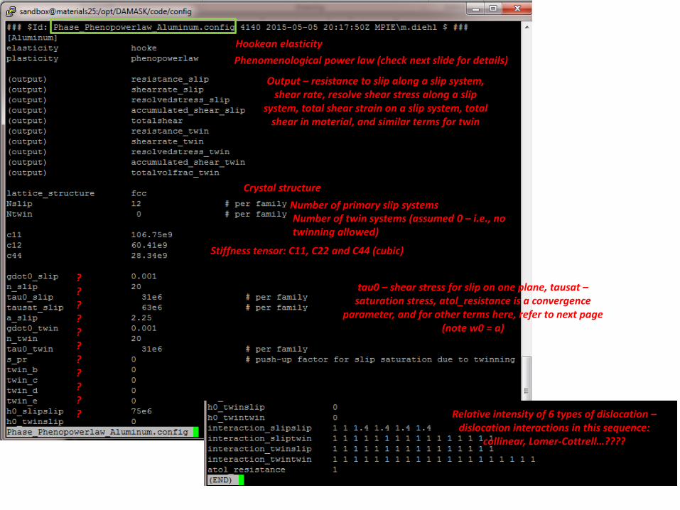
<phase> {/opt/DAMASK/code/config/Phase_Phenopowerlaw_Aluminum.config}

This is the routine (at /opt/… location)

To define load file – let’s use “nano” command to create a file called “tensionY.load”

1. * represents unconstrained BC 2. Strain rate in y direction is 10-3 s-1

3. Stress in x-direction must be zero (traction free)

4. Load it for 100 seconds (i.e., up to 0.1 strain) 5. Total increments to finish is 200 (i.e. each

time step is of 0.5 seconds) 6. Save data with frequency of 5 – so total 40

sets of data will be saved

I

II

Do not write it with “new lines”

More than one loading sequence can be applied by

writing “all loading /boundary conditions

commands” in different lines (first line is first set of

loading, etc.)

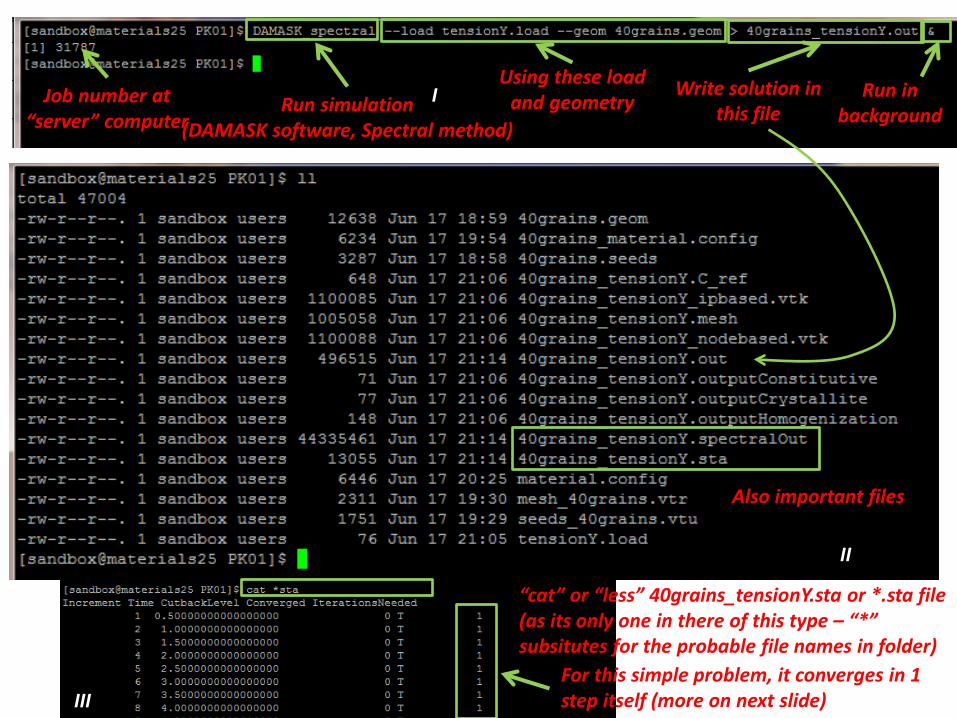
Run simulation (DAMASK software, Spectral method)

Using these load and geometry

Write solution in this file

Run in background

Job number at “server” computer

Also important files

“cat” or “less” 40grains_tensionY.sta or *.sta file (as its only one in there of this type – “*” subsitutes for the probable file names in folder)

For this simple problem, it converges in 1 step itself (more on next slide)

I

II

III

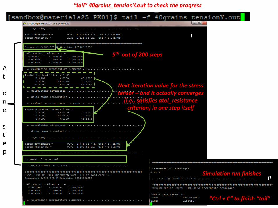
“tail” 40grains_tensionY.out to check the progress

5th out of 200 steps

Next iteration value for the stress tensor – and it actually converges

(i.e., satisfies atol_resistance criterion) in one step itself

At one step

Simulation run finishes

“Ctrl + C” to finish “tail”

I

II

-- cr (crystallite outputs check in .config file for

options) Write – f and p

Creates a folder postProc with text file containing “average of all load steps” f and p results (no time resolution here)

II

I

Change directory (cd) to postProc and then long list items in there

Working directory (pwd)

Txt file has all data in table with these “labels”

Add (Left Cauchy-Green) strain tensor in table from the displacement gradient tensor

--left (left strain tensor), --logarithmic (true strain)

2-D tensors of f and p are written row-wise so axy is (2*(x-1)+y)_a

Add (calculate) Cauchy stress tensor from first Piola-Kirchhoff stress tensor

Generate Mises strain using Left Cauchy-Green Strain and Cauchy Stress Tensors and Add it to table

II

I

III

IV

showTable (shows table), showTable --abc Shows a component of the table

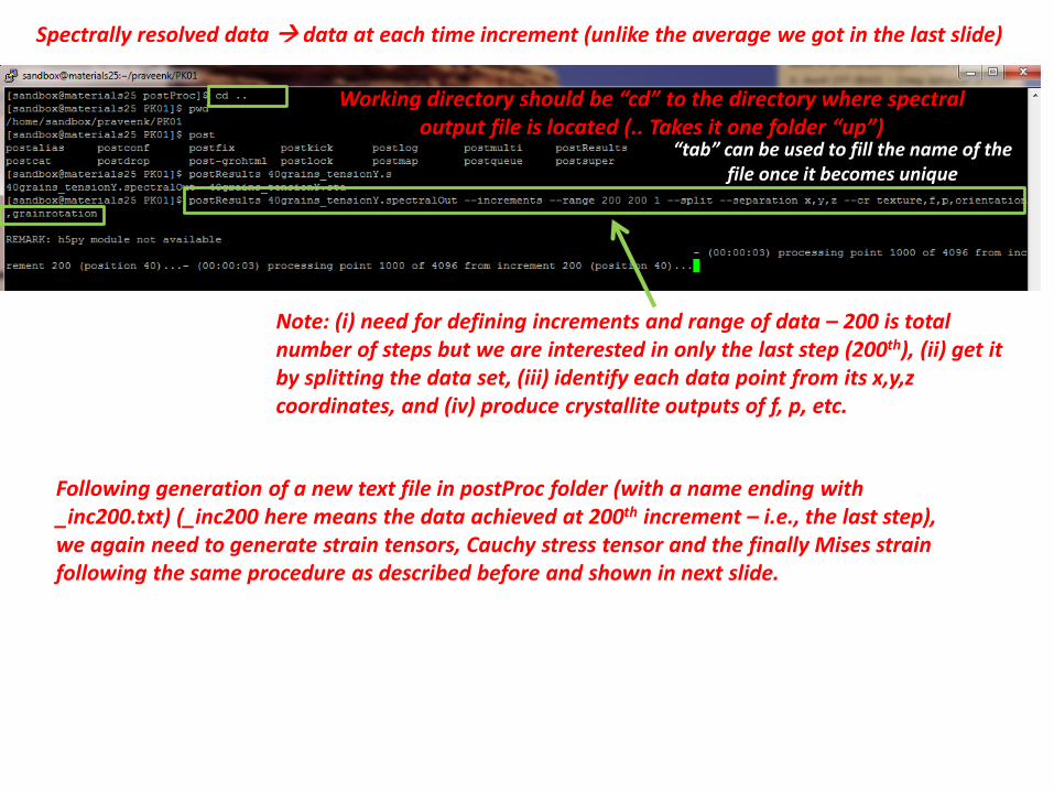
Spectrally resolved data data at each time increment (unlike the average we got in the last slide)

Working directory should be “cd” to the directory where spectral output file is located (.. Takes it one folder “up”)

“tab” can be used to fill the name of the file once it becomes unique

Note: (i) need for defining increments and range of data – 200 is total number of steps but we are interested in only the last step (200th), (ii) get it by splitting the data set, (iii) identify each data point from its x,y,z coordinates, and (iv) produce crystallite outputs of f, p, etc.

Following generation of a new text file in postProc folder (with a name ending with _inc200.txt) (_inc200 here means the data achieved at 200th increment – i.e., the last step), we again need to generate strain tensors, Cauchy stress tensor and the finally Mises strain following the same procedure as described before and shown in next slide.

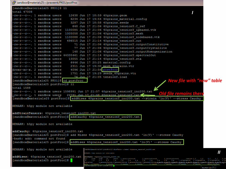
New file with “new” table

Old file remains there

II

I

Inverse pole figures with (001) pole in cubic system

Initial Geometry IPF after loading

Produces an image with “RGB” colours

Take data from time table under given lable

Dimension of data is 64 x

64

Transfer it to your computer from server computer for viewing

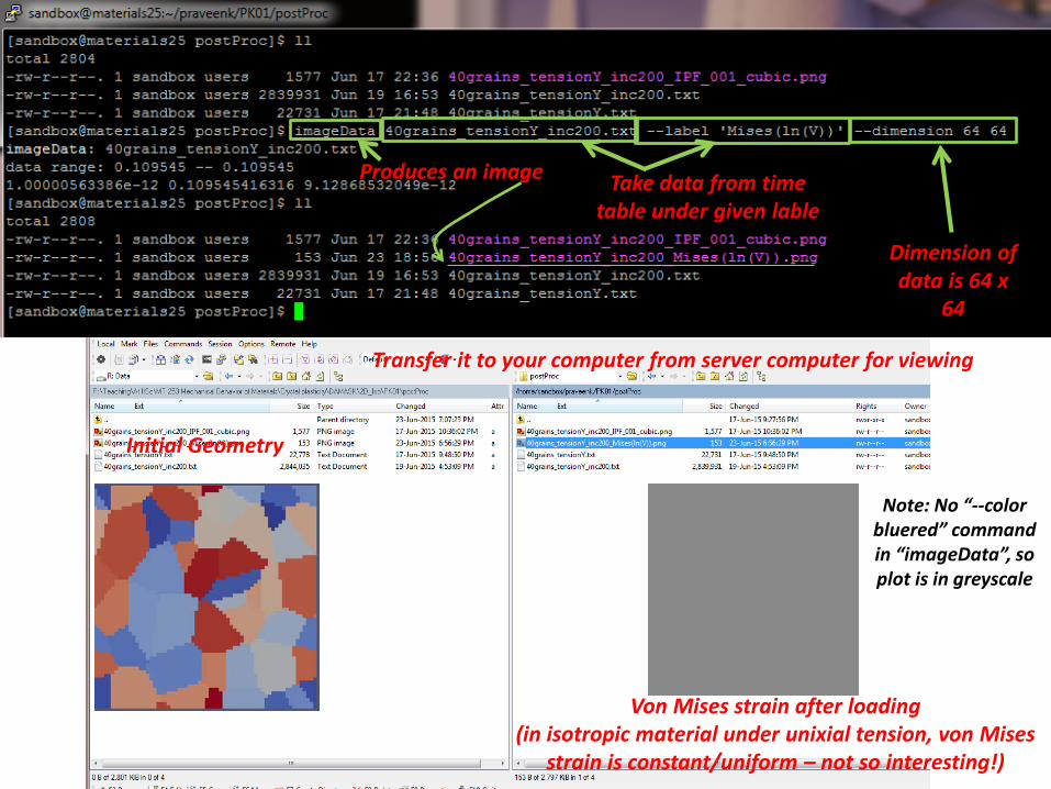
Initial Geometry

Von Mises strain after loading (in isotropic material under unixial tension, von Mises

strain is constant/uniform – not so interesting!)

Produces an image Take data from time table under given lable

Transfer it to your computer from server computer for viewing

Dimension of data is 64 x

64

Note: No “--color bluered” command in “imageData”, so plot is in greyscale

Make a new directory (in this case PK_02), go there and copy geometry, configuration, visualization (vtu & vtr) and load files from praveenk/PK_01 to this directory

Copy (cp) this file from location PK01 which is in one level up directory (../PK01)

Copy here in this directory (i.e., PK02)

Tutorial 2: Uniaxial tension type loading on a crystalline material (specific slip systems, etc.)

Editing “material.config” file to change the materials model from “isotropic” to

“Phenomenological power law”

I

II

Hookean elasticity Phenomenological power law (check next slide for details)

Output – resistance to slip along a slip system, shear rate, resolve shear stress along a slip

system, total shear strain on a slip system, total shear in material, and similar terms for twin

Stiffness tensor: C11, C22 and C44 (cubic)

tau0 – shear stress for slip on one plane, tausat – saturation stress, atol_resistance is a convergence

parameter, and for other terms here, refer to next page (note w0 = a)

Crystal structure Number of primary slip systems Number of twin systems (assumed 0 – i.e., no twinning allowed)

??????????? Relative intensity of 6 types of dislocation –

dislocation interactions in this sequence: collinear, Lomer-Cottrell…????

Run simulation (DAMASK software, Spectral method)

Using these load and geometry Write solution in

this file Run in

background Job number at

“server” computer

Also important files

I

“tail” 40grains_tensionY.out to check the progress

10th out of 200 steps

Next iteration value for the stress tensor – it may take a few more

steps

At one step

Simulation run finishes

“Ctrl + C” to finish “tail”

I

II

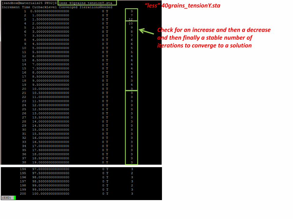
“less” 40grains_tensionY.sta

Check for an increase and then a decrease and then finally a stable number of iterations to converge to a solution

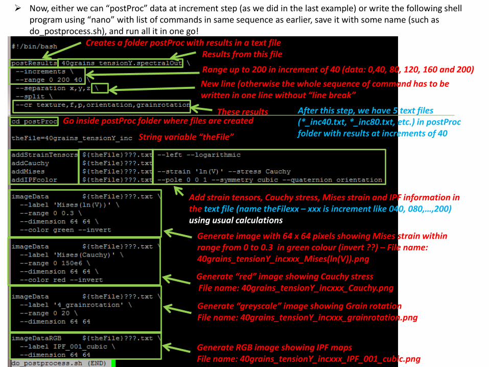
Now, either we can “postProc” data at increment step (as we did in the last example) or write the following shell program using “nano” with list of commands in same sequence as earlier, save it with some name (such as do_postprocess.sh), and run all it in one go!

Creates a folder postProc with results in a text file Results from this file

New line (otherwise the whole sequence of command has to be written in one line without “line break”

Range up to 200 in increment of 40 (data: 0,40, 80, 120, 160 and 200)

These results After this step, we have 5 text files (*_inc40.txt, *_inc80.txt, etc.) in postProc folder with results at increments of 40

Go inside postProc folder where files are created

String variable “theFile”

Add strain tensors, Cauchy stress, Mises strain and IPF information in the text file (name theFilexx – xxx is increment like 040, 080,…,200) using usual calculations

Generate image with 64 x 64 pixels showing Mises strain within range from 0 to 0.3 in green colour (invert ??) – File name: 40grains_tensionY_incxxx_Mises(ln(V)).png

Generate “red” image showing Cauchy stress File name: 40grains_tensionY_incxxx_Cauchy.png

Generate “greyscale” image showing Grain rotation File name: 40grains_tensionY_incxxx_grainrotation.png

Generate RGB image showing IPF maps File name: 40grains_tensionY_incxxx_IPF_001_cubic.png

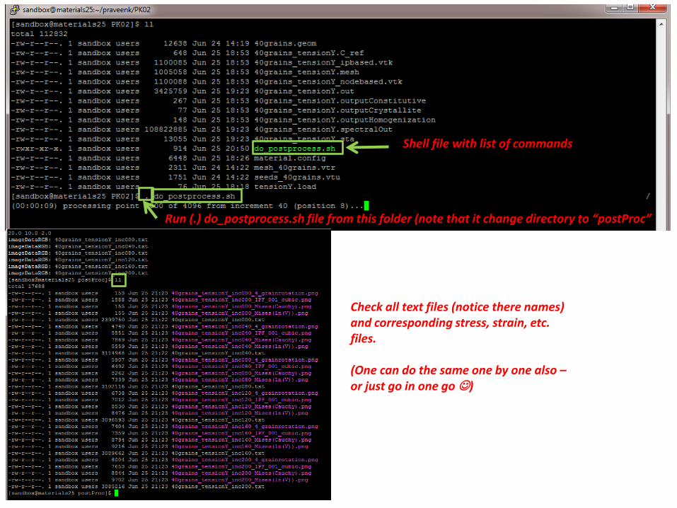
Shell file with list of commands

Run (.) do_postprocess.sh file from this folder (note that it change directory to “postProc”

Check all text files (notice there names) and corresponding stress, strain, etc. files. (One can do the same one by one also – or just go in one go )

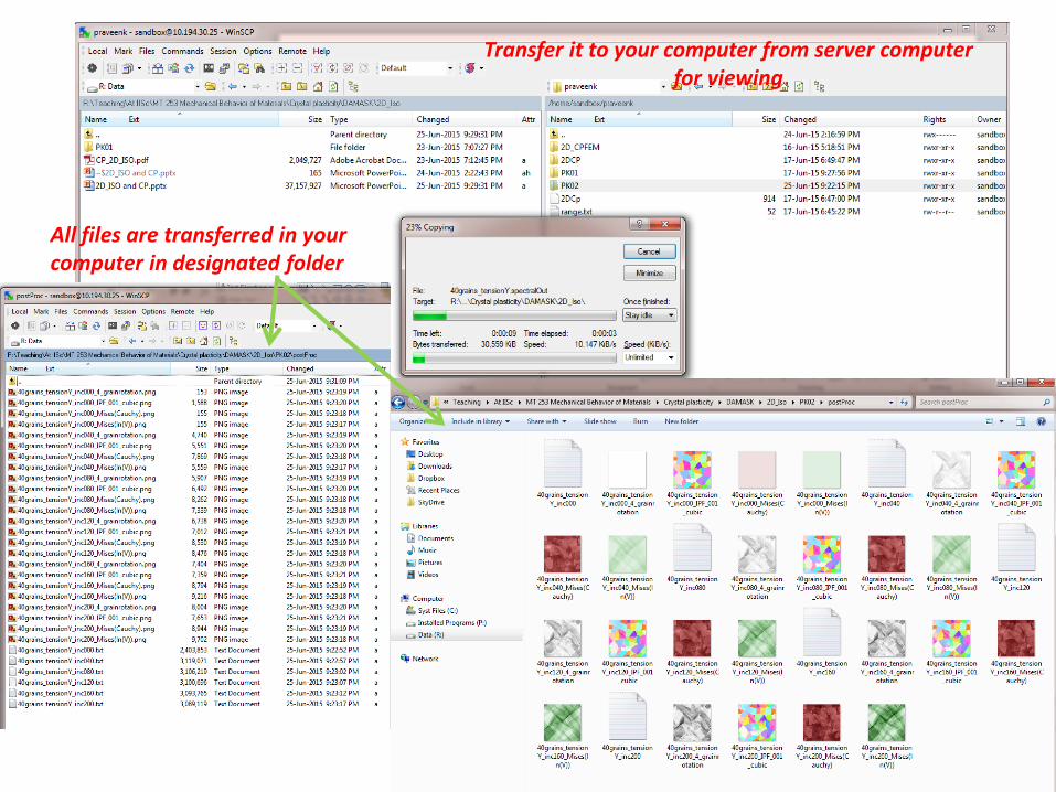
Transfer it to your computer from server computer for viewing

All files are transferred in your computer in designated folder

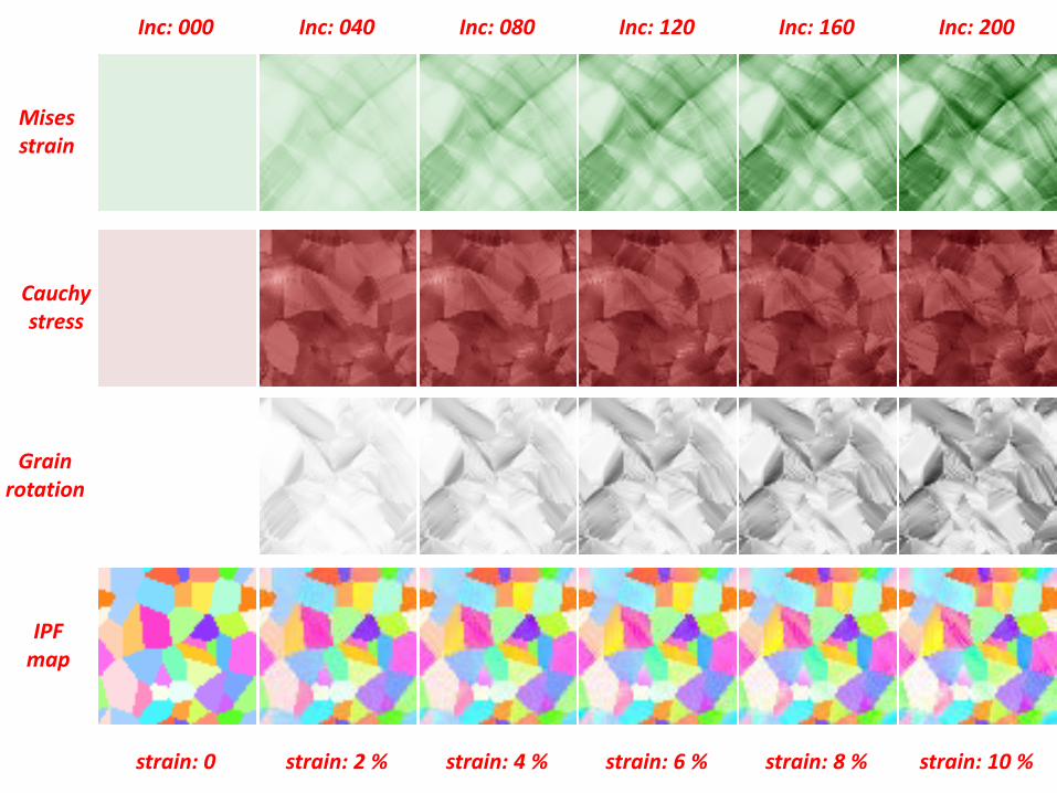
Mises strain

Inc: 000 Inc: 080 Inc: 120 Inc: 160 Inc: 200 Inc: 040

Cauchy stress

Grain rotation

IPF map

strain: 0 strain: 2 % strain: 4 % strain: 6 % strain: 8 % strain: 10 %

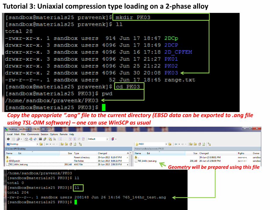
Copy the appropriate “.ang” file to the current directory (EBSD data can be exported to .ang file using TSL-OIM software) – one can use WinSCP as usual

Geometry will be prepared using this file

Tutorial 3: Uniaxial compression type loading on a 2-phase alloy

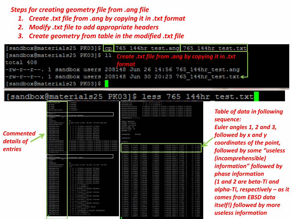
Steps for creating geometry file from .ang file 1. Create .txt file from .ang by copying it in .txt format 2. Modify .txt file to add appropriate headers 3. Create geometry from table in the modified .txt file

Create .txt file from .ang by copying it in .txt format

Commented details of entries

Table of data in following sequence: Euler angles 1, 2 and 3, followed by x and y coordinates of the point, followed by some “useless (incomprehensible) information” followed by phase information (1 and 2 are beta-Ti and alpha-Ti, respectively – as it comes from EBSD data itself!) followed by more useless information

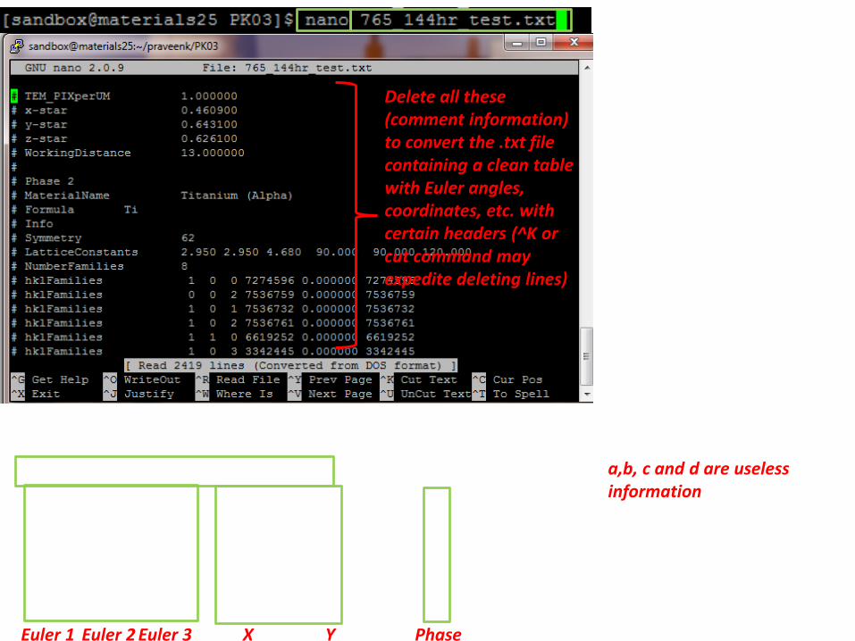
Delete all these (comment information) to convert the .txt file containing a clean table with Euler angles, coordinates, etc. with certain headers (^K or cut command may expedite deleting lines)

a,b, c and d are useless information

Euler 1 X Euler 3 Euler 2 Y Phase

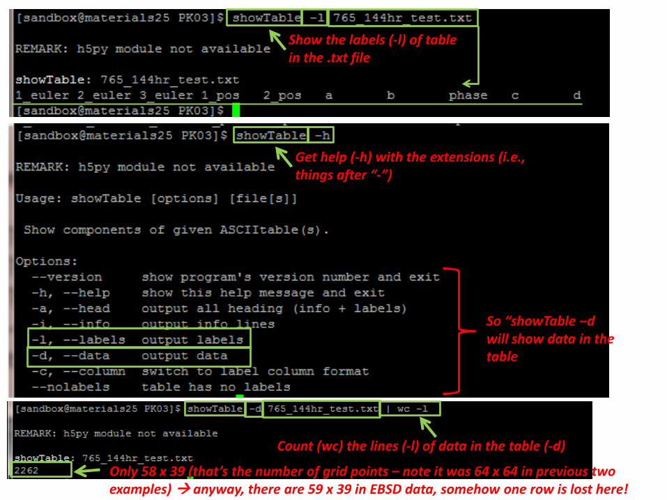
Show the labels (-l) of table in the .txt file

Get help (-h) with the extensions (i.e., things after “-”)

So “showTable –d will show data in the table

Count (wc) the lines (-l) of data in the table (-d)

Only 58 x 39 (that’s the number of grid points – note it was 64 x 64 in previous two examples) anyway, there are 59 x 39 in EBSD data, somehow one row is lost here!

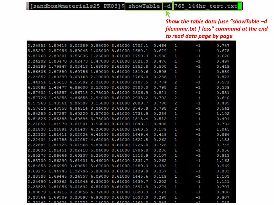
Show the table data (use “showTable –d filename.txt | less” command at the end to read data page by page

Get help (-h or --help) with the extensions (i.e., things after “-”)

????

First row data of Euler angles

Filter all Euler angles (?_euler) data from the first row of the table (#_row_# == 1) --? – what is the use of this step?

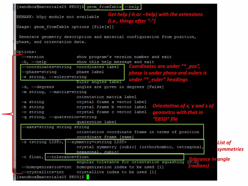
Get help (-h or --help) with the extensions (i.e., things after “-”)

Coordinates are under “*_pos”, phase is under phase and eulers is under “*_euler” headings

Orientation of x, y and z of geometru with that in “EBSD” file

List of symmetries

Tolerance in angle (radians)

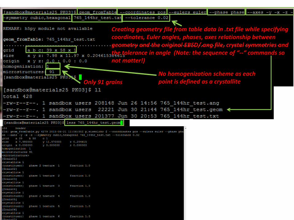
Creating geometry file from table data in .txt file while specifying coordinates, Euler angles, phases, axes relationship between geometry and the original EBSD/.ang file, crystal symmetries and the tolerance in angle (Note: the sequence of “--“ commands so not matter!)

Only 91 grains No homogenization scheme as each point is defined as a crystallite

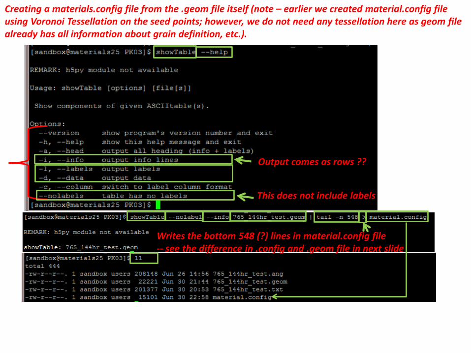
Creating a materials.config file from the .geom file itself (note – earlier we created material.config file using Voronoi Tessellation on the seed points; however, we do not need any tessellation here as geom file already has all information about grain definition, etc.).

This does not include labels

Output comes as rows ??

Writes the bottom 548 (?) lines in material.config file -- see the difference in .config and .geom file in next slide

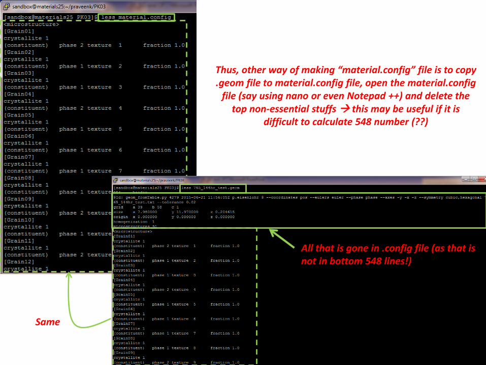
All that is gone in .config file (as that is not in bottom 548 lines!)

Same

Thus, other way of making “material.config” file is to copy .geom file to material.config file, open the material.config

file (say using nano or even Notepad ++) and delete the top non-essential stuffs this may be useful if it is

difficult to calculate 548 number (??)

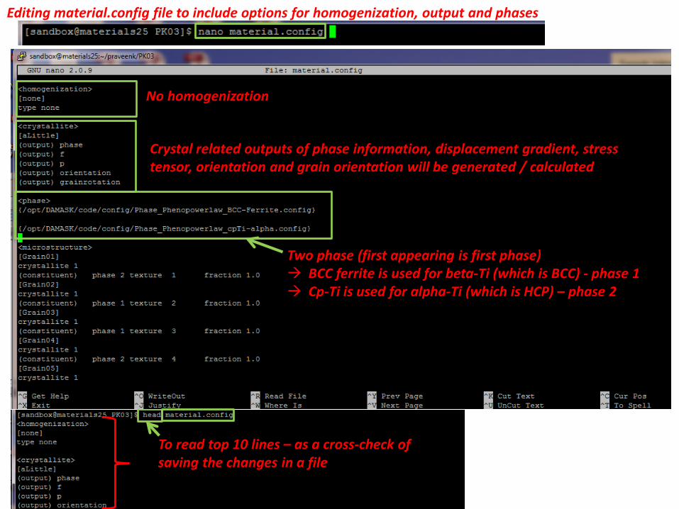
Editing material.config file to include options for homogenization, output and phases

No homogenization

Crystal related outputs of phase information, displacement gradient, stress tensor, orientation and grain orientation will be generated / calculated

Two phase (first appearing is first phase) BCC ferrite is used for beta-Ti (which is BCC) - phase 1 Cp-Ti is used for alpha-Ti (which is HCP) – phase 2

To read top 10 lines – as a cross-check of saving the changes in a file

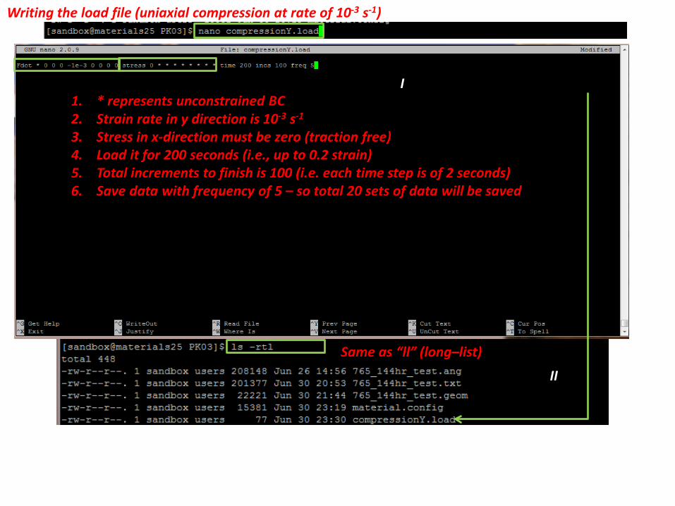
Writing the load file (uniaxial compression at rate of 10-3 s-1)

1. * represents unconstrained BC 2. Strain rate in y direction is 10-3 s-1

3. Stress in x-direction must be zero (traction free) 4. Load it for 200 seconds (i.e., up to 0.2 strain) 5. Total increments to finish is 100 (i.e. each time step is of 2 seconds) 6. Save data with frequency of 5 – so total 20 sets of data will be saved

I

II

Same as “ll” (long–list)

Running DAMASK Simulation on more than 1 node ()

How many nodes are available How many are used by DAMASK now Run DAMASK on 4 nodes

Run simulation Using these load

and geometry Write solution in

this file Run in

background Job number at

“server” computer

Follow as the simulation runs

(on 4 nodes, it will run very fast)

Could not converge beyond 80 steps (i.e., slightly less

than 16 % strain)

Cut back exceeded ??

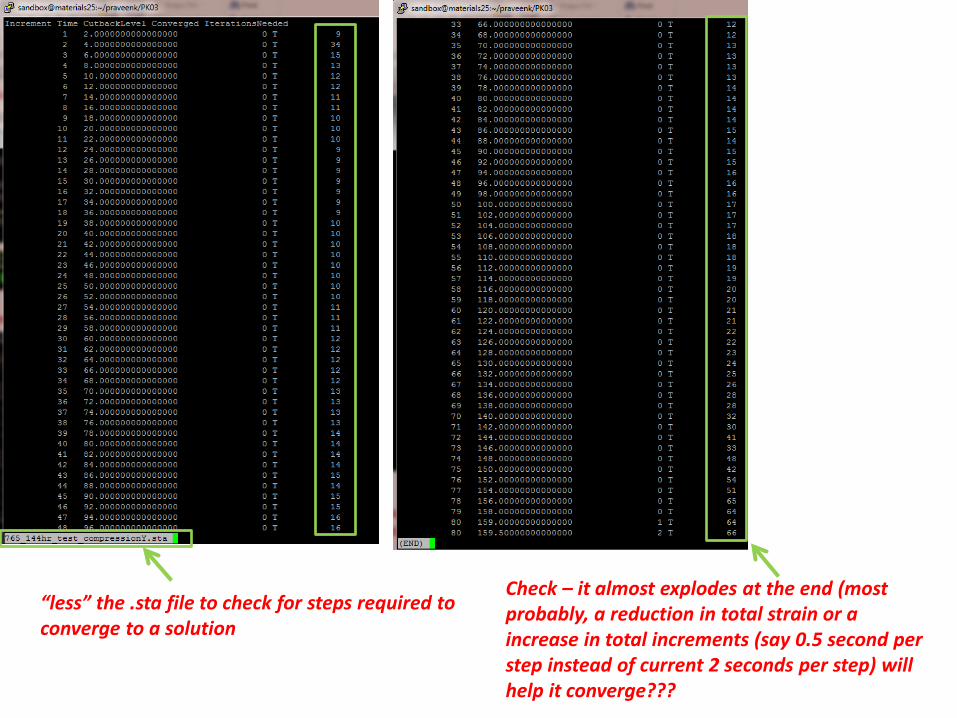
“less” the .sta file to check for steps required to converge to a solution

Check – it almost explodes at the end (most probably, a reduction in total strain or a increase in total increments (say 0.5 second per step instead of current 2 seconds per step) will help it converge???

We can use the same old shell program to do post processing for us – however, we need to modify it to suit this problem (look at range, only two question marks in file name (i.e., ?? Instead of ???), and assigning the proper name to IPF maps based on their phase number. We can edit using “nano” in “putty” or text editor in “windows”

Windows – editing using Notepad ++

Transfer it to server using winSCP

I

II

III

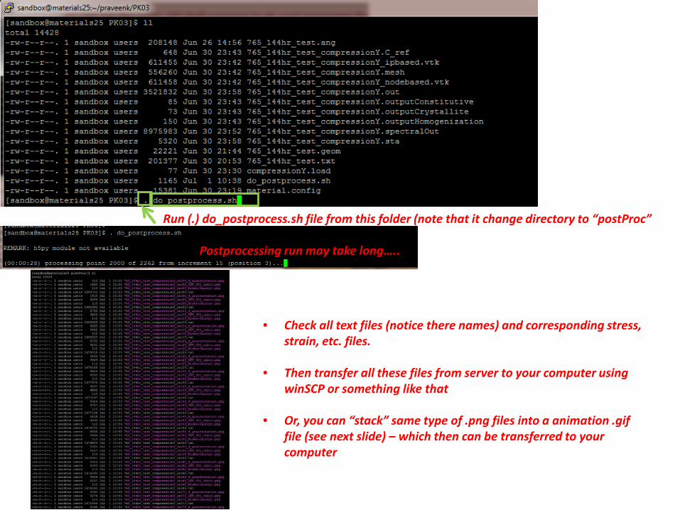
Run (.) do_postprocess.sh file from this folder (note that it change directory to “postProc”

• Check all text files (notice there names) and corresponding stress, strain, etc. files.

• Then transfer all these files from server to your computer using winSCP or something like that

• Or, you can “stack” same type of .png files into a animation .gif file (see next slide) – which then can be transferred to your computer

Postprocessing run may take long…..

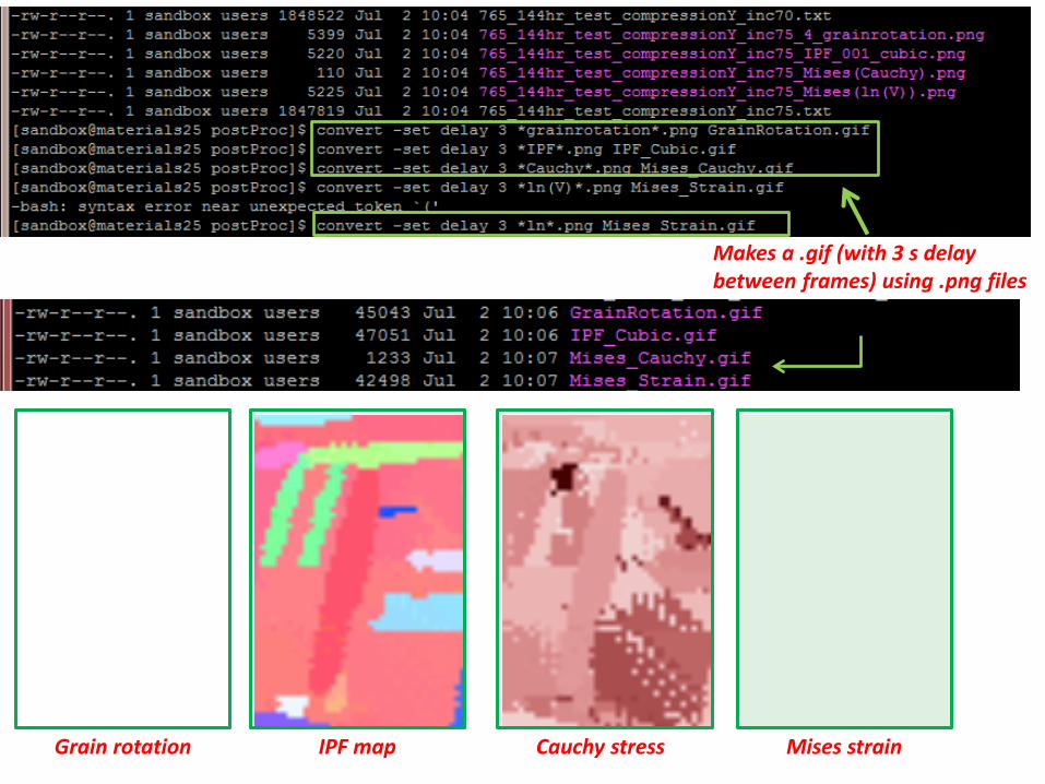
Makes a .gif (with 3 s delay between frames) using .png files

Grain rotation IPF map Cauchy stress Mises strain