A Two-Stage Hybrid Local Search

for the Vehicle Routing Problem with Time Windows1

Russell Bent and Pascal Van Hentenryck

Brown UniversityBox 1910, Providence, RI 02912

Abstract

The vehicle routing problem with time windows is a hard combinatorial optimization problemwhich has received considerable attention in the last decades. This paper proposes a two-stagehybrid algorithm for this transportation problem. The algorithm �rst minimizes the number ofvehicles using simulated annealing. It then minimizes travel cost using a large neighborhoodsearch which may relocate a large number of customers. Experimental results demonstrate thee�ectiveness of the algorithm which has improved 13 (23%) of the 58 best published solutions tothe Solomon benchmarks, while matching or improving the best solutions in 47 problems (84%).More important perhaps, the algorithm is shown to be very robust. With a �xed con�gurationof its parameters, it returns either the best published solutions (or improvements thereof) orsolutions very close in quality on all Solomon benchmarks. Results on the extended Solomonbenchmarks are also given.

1 Introduction

Vehicle routing problems are important components of many distribution and transportation sys-tems, including such examples as bank deliveries, postal deliveries, school bus routing, and securitypatrol services. They have received considerable attention in the past decades. This paper con-siders the vehicle routing problem with time windows (VRPTW). Given a number of customerswith known demands and a eet of identical vehicles with known capacities, the problem consists of�nding a set of routes originating and terminating at a central depot and servicing all the customersexactly once. The routes cannot violate the capacity constraints on the vehicles and, in addition,must meet the time windows of the customers, which specify the earliest and latest times for thestart of service at a customer site. The standard objective of the VRPTW problem consists of min-imizing the number of routes or vehicles (primary criterion) and the total travel cost (secondarycriterion). The VRPTW problem is NP-complete [21] and instances involving 100 customers ormore are very hard to solve optimally. Indeed, very few of the traditional benchmarks [29] involving100 customers been solved optimally (See [9, 20] for some recent results). As a consequence, localsearch techniques are often used to �nd good solutions in reasonable time.

This paper presents a two-stage hybrid algorithm for the VRPTW problem. The overall struc-ture of the algorithm is motivated by the recognition that minimizing the objective function directlymay not be the most e�ective way to decrease the number of routes. Indeed, the objective func-tion often drives the search toward solutions with low travel cost, which may make it diÆcult toreach solutions with fewer routes but higher travel cost. To overcome this limitation, our algorithmdivides the search in two steps:

1Technical Report, CS-01-06, Department of Computer Science, Brown University, September 2001.

1

1. the minimization of the number of routes;

2. the minimization of travel cost.

This two-step approach makes it possible to design algorithms tailored to each sub-optimization.The only other two stage algorithm we are aware of is reference [15], where the same evolutionarymetaheuristic is used with two distinct objective functions to approach the two subproblems. Ouralgorithm uses two distinct local search procedures to exploit the speci�cities of each subproblem.Indeed, the �rst step of our algorithm uses simulated annealing to minimize the number of routes.One critical aspect of our simulated annealing algorithm is its lexicographic evaluation functionwhich minimizes the number of routes (primary criterion), maximizes the sum of the squares ofthe route sizes (secondary criterion), and minimizes minimal delay [15] of the routing plan (thirdcriterion). The second criterion was also successfully used in other applications (e.g., graph coloring[17]). The second step of our algorithm uses a large neighborhood search (LNS) [28] to minimizetotal travel cost. It is motivated by our belief that LNS is particularly e�ective in minimizingtotal travel cost when given a solution that minimizes the number of routes. Note also that ourimplementation of LNS makes it very close to variable neighborhood search [13].

Experimental results demonstrate the e�ectiveness of the algorithm. On the standard Solomonbenchmarks, the algorithm improved the best published solutions in 13 of the 56 problems (23%)and matches or improves the best published results in 47 problems (84%). More important perhaps,the experimental results highlight the robustness of the algorithm. With a standard con�gurationof its parameters, the algorithm consistently returns either the best published solutions (or im-provements thereof) or solutions that are very close in quality.

The rest of this paper is organized as follows. Section 2 describes the problem formulation andspeci�es the notations used in the paper. Section 3 gives an overview of the overall algorithm.Section 4 presents the simulated annealing algorithm for minimizing routes, while Section 5 de-scribes the LNS algorithm for minimizing travel costs. Section 6 presents the experimental results.Section 7 discusses related work and Section 8 concludes the paper. The appendix contains theimprovements over the best solutions found during the course of this research.

2 Problem Formulation and De�nitions

This section de�nes the vehicle routing problem with time windows (VRPTW) and the variousconcepts used in this paper.

Customers The problem is de�ned in terms of N customers who are represented by the numbers1; : : : ; N and a depot represented by the number 0. The set f0; 1; : : : ; Ng thus represents all thesites considered in the problem. We also use Customers to represent the set of customers and Sitesto represent the set of sites. The travel cost between sites i and j is denoted by cij . Travel costssatisfy the triangular inequality

cij + cjk � cik:

2

The normalized travel cost c0ij between sites i and j is de�ned as

c0ij = cij = maxi;j2Sites

cij :

Every customer i has a demand qi � 0 and a service time si � 0.

Vehicles The VRPTW problem is de�ned in terms of m identical vehicles. Each vehicle has acapacity Q.

Routes A vehicle route, or route for short, starts from the depot, visits a number of customersat most once, and returns to the depot. In other words, a route is a sequence h0; v1; : : : ; vn; 0i orhv1; : : : ; vni for short, where all vi are di�erent. The customers of a route r = hv1; : : : ; vni, denotedby cust(r), is the set fv1; : : : ; vng. The size of a route, denoted by jrj, is the number of customersjcust(r)j. The demand of a route, denoted by q(r), is the sum of the demands of its customers, i.e.,

q(r) =X

c2cust(r)

qc:

A route satis�es its capacity constraint if

q(r) � Q:

The travel cost of a route r = hv1; : : : ; vni, denoted by t(r), is the cost of visiting all its customers,i.e.,

t(r) = c0v1 + cv1v2 + : : : + cvn�1vn + cvn0:

if the route is not empty (n � 1) and is zero otherwise.

Routing Plan A routing plan is a set of routes fr1; : : : ; rmg (m � M) visiting every customerexactly once, i.e., ( Sm

i=1 cust(ri) = Customerscust(ri) \ cust(rj) = ; (1 � i < j � m)

Observe that a routing plan assigns a unique successor and predecessor to every customer. Thesesuccessors and predecessors are sites. The successor and predecessor of customer i in routing plan �are denoted by succ(i; �) and pred (i; �). For simplicity, our de�nitions often assume an underlyingrouting plan � and we use i+ and i� to denote the successor and predecessor of i in �.

Time Windows The customers and the depot have time windows. The time window of a site i isspeci�ed by an interval [ei; li], where ei represents the earliest and latest arrival times respectively.Vehicles must arrive at a site before the end of the time window li. They may arrive early but theyhave to wait until time ei to be serviced. Observe that e0 represents the time when all vehicles in

3

the routing plan leave the depot and that l0 represents the time when they must all return to thedepot. The departure time of customer i, denoted by Æi, is de�ned recursively as(

Æ0 = 0Æi = max(Æi� + ci�i ; ei) + si (i 2 Customers):

The earliest service time of customer i, denoted by ai, is de�ned as

ai = max(Æi� + ci�i ; ei) (i 2 Customers):

The earliest arrival time of a route r = hv1; : : : ; vni, denoted by a(r), is given by Ævn + cvn0 ifthe route is not empty and is e0 otherwise. A routing plan satis�es the time window constraintfor customer i if ai � li: A routing plan � satis�es the time window constraint for the depot if8r 2 � : a(r) � l0: The latest arrival time for customer i which does not violate the time windowconstraints of i and the customers served after i on its route, denoted by zi, is de�ned recursivelyas (

z0 = l0zi = min(zi+ � cii+ � si ; li) (i 2 Customers):

The VRPTW Problem A solution to the VRPTW problem is a routing plan � = fr1; : : : ; rmgsatisfying the capacity constraints and the time window constraints, i.e.,8><

>:q(rj) � Q (1 � j � m)a(rj) � l0 (1 � j � m)ai � li (i 2 Customers)

The size of a routing plan �, denoted by j�j, is the number of non-empty routes in �, i.e.,

jfr 2 � j cust(r) 6= ;g:

The VRPTW problem consists of �nding a solution � which minimizes the number of vehicles and,in case of ties, the total travel cost, i.e., a solution � minimizing the objective function speci�ed bythe lexicographic order

f(�) = hj�j;Xr2�

t(r)i:

3 Overview of the Algorithm

As mentioned in the introduction, our algorithm is motivated by the recognition that minimizingthe objective function

hj�j;Xr2�

t(r)i:

is not always the most e�ective way to approach the problem. Indeed, the objective function oftendrives the search towards solutions with low travel costs. The reduction in the number of routes

4

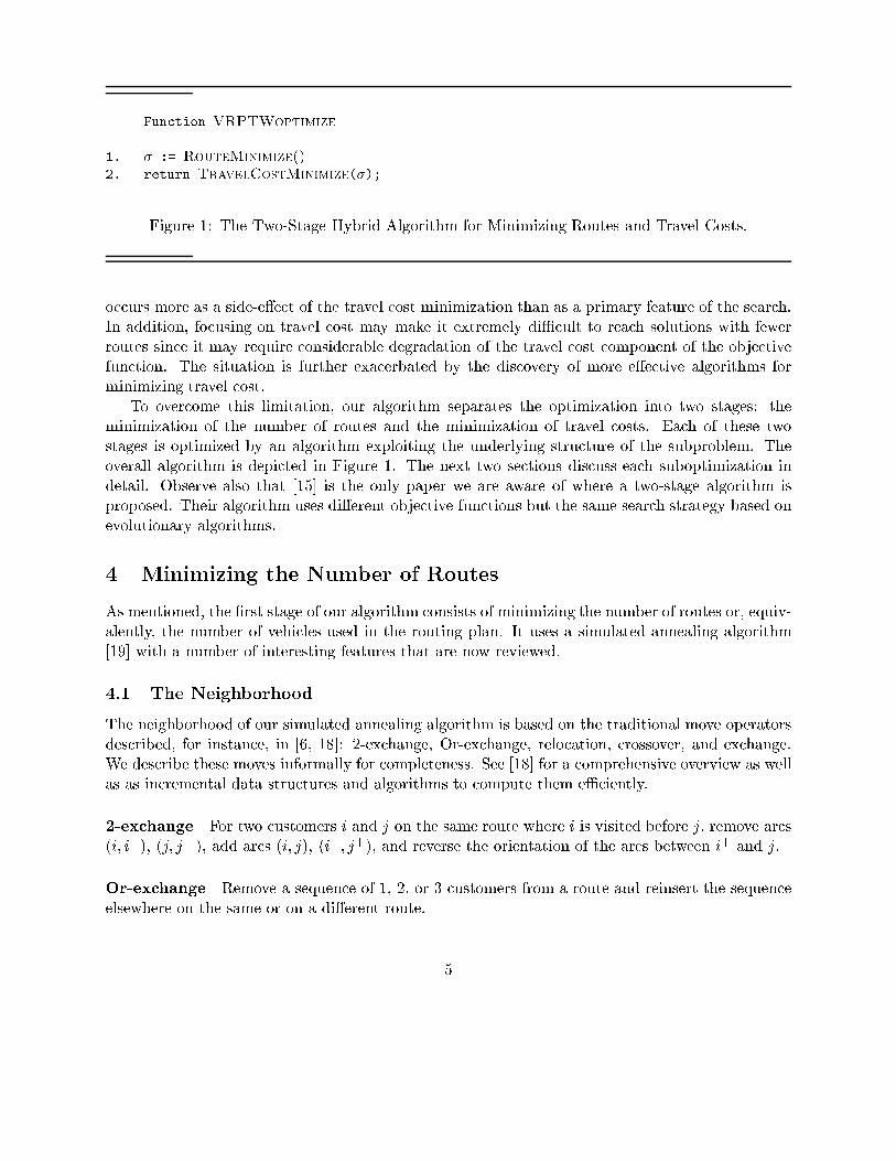
Function VRPTWoptimize

1. � := RouteMinimize()2. return TravelCostMinimize(�);

Figure 1: The Two-Stage Hybrid Algorithm for Minimizing Routes and Travel Costs.

occurs more as a side-e�ect of the travel cost minimization than as a primary feature of the search.In addition, focusing on travel cost may make it extremely diÆcult to reach solutions with fewerroutes since it may require considerable degradation of the travel cost component of the objectivefunction. The situation is further exacerbated by the discovery of more e�ective algorithms forminimizing travel cost.

To overcome this limitation, our algorithm separates the optimization into two stages: theminimization of the number of routes and the minimization of travel costs. Each of these twostages is optimized by an algorithm exploiting the underlying structure of the subproblem. Theoverall algorithm is depicted in Figure 1. The next two sections discuss each suboptimization indetail. Observe also that [15] is the only paper we are aware of where a two-stage algorithm isproposed. Their algorithm uses di�erent objective functions but the same search strategy based onevolutionary algorithms.

4 Minimizing the Number of Routes

As mentioned, the �rst stage of our algorithm consists of minimizing the number of routes or, equiv-alently, the number of vehicles used in the routing plan. It uses a simulated annealing algorithm[19] with a number of interesting features that are now reviewed.

4.1 The Neighborhood

The neighborhood of our simulated annealing algorithm is based on the traditional move operatorsdescribed, for instance, in [6, 18]: 2-exchange, Or-exchange, relocation, crossover, and exchange.We describe these moves informally for completeness. See [18] for a comprehensive overview as wellas as incremental data structures and algorithms to compute them eÆciently.

2-exchange For two customers i and j on the same route where i is visited before j, remove arcs(i; i+), (j; j+), add arcs (i; j), (i+; j+), and reverse the orientation of the arcs between i+ and j.

Or-exchange Remove a sequence of 1, 2, or 3 customers from a route and reinsert the sequenceelsewhere on the same or on a di�erent route.

5

Relocation For customers i and j, place i after j, i.e., remove arcs (i�; i), (i; i+), (j; j+) and addarcs (i�; i+), (j; i), and (i; j+).

Exchange Exchange the positions of customers i and j, i.e., remove (i�; i), (i; i+), (j�; j), (j; j+)and add (i�; j), (j; i+), (j�; i), (i; j+).

Crossover Exchange the successors of customers i and j, i.e., remove (i; i+), (j; j+) and add(i; j+), (j; i+).

Given a solution �, N (�) denotes the neighborhood of �, i.e., the set of solutions that can bereached from � by using one of these move operators. We also denote by Operators the set of moveoperators f2-exchange, Or-exchange, relocation, exchange, crossoverg.

A Random Sub-Neighborhood One of the interesting features of our simulated annealingalgorithm is how it explores the neighborhood. Indeed, each iteration of the algorithm focuseson a (random) sub-neighborhood of N obtained by randomly choosing a move operator o fromOperators and a customer c from Customers and by constructing all the moves using operator oand customer c. The sub-neighborhood will be explored exhaustively to �nd whether it containsa solution improving the best available routing plan and to choose the next move. We denote byN (o; c; �) the subset of N (�) that can be reached by using move operator o and customer c.

4.2 The Evaluation Function

The evaluation function is another fundamental aspect of our simulated annealing algorithm. Asmentioned earlier, the objective function

hj�j;Xr2�

t(r)i:

is not always appropriate, since it may lead the search to solutions with a small travel cost andmakes it impossible to remove routes. To overcome this limitation, our simulated algorithm uses amore complex lexicographic ordering

e(�) = hj�j;�Xr2�

jrj2;mdl(�)i:

especially tailored to minimize the number of routes. The �rst component is of course the numberof routes. The second component maximizes X

r2�

jrj2

which means that it favors solutions containing routes with many customers and routes with fewcustomers over solutions where customers are distributed more evenly among the routes. Theintuition is to guide the algorithm into removing customers from some small routes and adding them

6

to larger routes. Components of this type are used in many algorithms, a typical example beinggraph coloring [17]. The third component minimizes the minimal delay of the routing plan. Thisconcept was introduced by [15] in the context of evolutionary algorithms. It favors solutions wherecustomers on the smallest route can be relocated on other routes with no constraint violations orwith time window violations which are as small as possible. Minimizing minimal delay thus favorssolutions where customers can be relocated more easily over solutions where relocation is hard.More precisely, the minimal delay is de�ned as follows:

De�nition 1 [Minimal Delay] The minimal delay of a solution �, denoted by mdl(�), is de�ned as

mdl(�) = mdl(r; �) where jrj = minr02�jr0j:

mdl(r; �) =P

i2cust(r)mdl(i; r; �):

mdl(i; r; �) =

8><>:

0 = if N (relocation ; i; �) 6= ;1 = if 8r0 2 r : r 6= r0 : q(r0) + qi > Q:minj2Customers n cust(r)mdl(i; j; r; �) otherwise.

mdl(i; j; r; �) = max(Æj + cji � li; 0) +max(Æi + cij+ � zj+; 0):

In other words, the minimal delay of a solution � is the minimal delay of the route with the smallestnumber of customers. The delay of a route is the summation of the delay of its customers. Theminimal delay of a customer i is 0 if i can be relocated on another route, 1 if i cannot be relocatedwithout violating the capacity constraints of the vehicle, or the minimal time window violationsinduced by relocating i after a customer j on another route. The time window violation is givenby the summation of the violation of the time window of i and the violation of the time window ofthe successors of j.

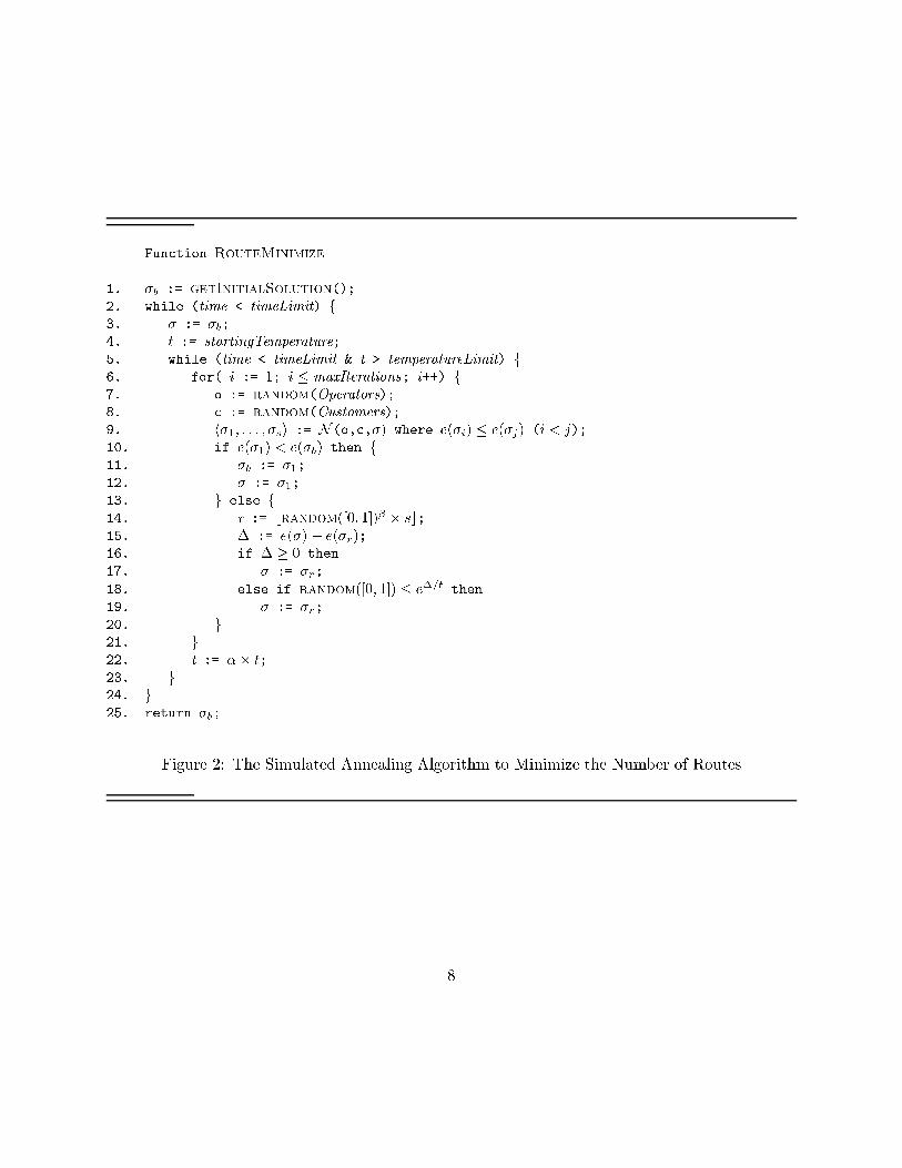
4.3 The Simulated Annealing Algorithm

Figure 2 depicts the simulated annealling algorithm. The algorithm consists of a number of localsearches (lines 3-23), each of which starts from the best solution found so far and from the startingtemperature. Each local search performs a number of iterations (lines 6-21) and decreases thetemperature (line 22). These two steps are repeated until the time limit is exhausted or thetemperature has reached its lower bound. Lines 7-20 describe one iteration and are most interesting.Lines 7-9 compute the sub-neighborhood

N (o; c; �) = h�1; : : : ; �si where e(�i) � e(�j) (i < j)

for a random move operator and a random customer. Lines 10-12 select the solution �1 minimizingf in N (o; c; �) if it improves the best solution found so far. These lines introduce an aspirationcriterion [12] in the simulated annealing algorithm. Lines 14-19 are the core of the algorithm. Line14 chooses a random element �r 2 N (o; c; �) and �r is selected as the nest routing plan if it doesnot degrade the current solution (line 16) or with the traditional probability of simulated annlealingotherwise (line 18). Observe also line 14

14. r := brandom([0; 1])� � sc;

which biases the search towards \good" moves in N (o; c; �) when � > 1.

7

Function RouteMinimize

1. �b := getInitialSolution();2. while (time < timeLimit) f3. � := �b;

4. t := startingTemperature;

5. while (time < timeLimit & t > temperatureLimit) f6. for( i := 1; i � maxIterations; i++) f7. o := random(Operators);8. c := random(Customers);

9. h�1; : : : ; �si := N(o,c,�) where e(�i) � e(�j) (i < j);

10. if e(�1) < e(�b) then f11. �b := �1;

12. � := �1;

13. g else f14. r := brandom([0; 1])� � sc;15. � := e(�) � e(�r);16. if � � 0 then

17. � := �r;

18. else if random([0; 1]) � e�=t then

19. � := �r;

20. g21. g22. t := �� t;

23. g24. g25. return �b;

Figure 2: The Simulated Annealing Algorithm to Minimize the Number of Routes

8

5 Minimizing the Travel Cost

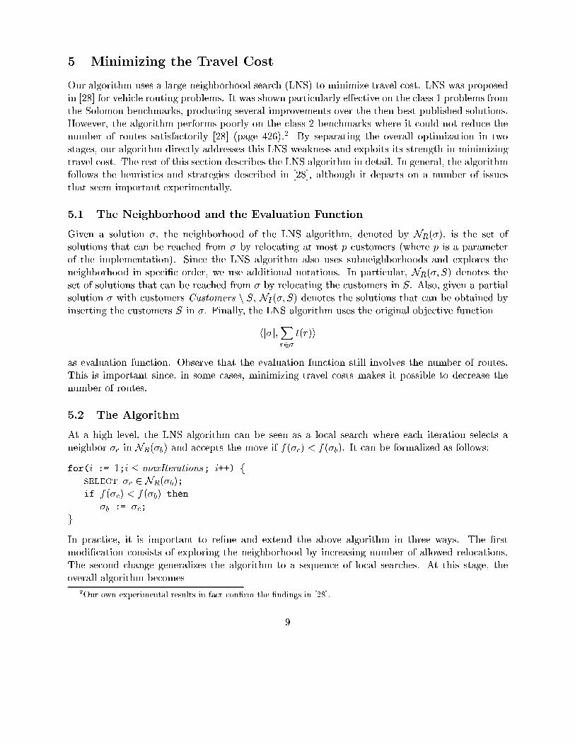
Our algorithm uses a large neighborhood search (LNS) to minimize travel cost. LNS was proposedin [28] for vehicle routing problems. It was shown particularly e�ective on the class 1 problems fromthe Solomon benchmarks, producing several improvements over the then best published solutions.However, the algorithm performs poorly on the class 2 benchmarks where it could not reduce thenumber of routes satisfactorily [28] (page 426).2 By separating the overall optimization in twostages, our algorithm directly addresses this LNS weakness and exploits its strength in minimizingtravel cost. The rest of this section describes the LNS algorithm in detail. In general, the algorithmfollows the heuristics and strategies described in [28], although it departs on a number of issuesthat seem important experimentally.

5.1 The Neighborhood and the Evaluation Function

Given a solution �, the neighborhood of the LNS algorithm, denoted by NR(�), is the set ofsolutions that can be reached from � by relocating at most p customers (where p is a parameterof the implementation). Since the LNS algorithm also uses subneighborhoods and explores theneighborhood in speci�c order, we use additional notations. In particular, NR(�; S) denotes theset of solutions that can be reached from � by relocating the customers in S. Also, given a partialsolution � with customers Customers n S, NI(�; S) denotes the solutions that can be obtained byinserting the customers S in �. Finally, the LNS algorithm uses the original objective function

hj�j;Xr2�

t(r)i

as evaluation function. Observe that the evaluation function still involves the number of routes.This is important since, in some cases, minimizing travel costs makes it possible to decrease thenumber of routes.

5.2 The Algorithm

At a high level, the LNS algorithm can be seen as a local search where each iteration selects aneighbor �c in NR(�b) and accepts the move if f(�c) < f(�b). It can be formalized as follows:

for(i := 1;i � maxIterations; i++) fselect �c 2 NR(�b);if f(�c) < f(�b) then

�b := �c;g

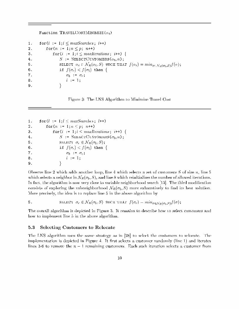
In practice, it is important to re�ne and extend the above algorithm in three ways. The �rstmodi�cation consists of exploring the neighborhood by increasing number of allowed relocations.The second change generalizes the algorithm to a sequence of local searches. At this stage, theoverall algorithm becomes

2Our own experimental results in fact con�rm the �ndings in [28].

9

Function TravelCostMinimize(�b)

1. for(l := 1;l � maxSearches; l++)2. for(n := 1;n � p; n++)3. for(i := 1;i � maxIterations; i++) f4. S := SelectCustomers(�b; n);5. select �c 2 NR(�b; S) such that f(�c) = min�2NR(�b ;S)f(�);

6. if f(�c) < f(�b) then f7. �b := �c;8. i := 1;9. g

Figure 3: The LNS Algorithm to Minimize Travel Cost

1. for(l := 1;l � maxSearches; l++)2. for(n := 1;n � p; n++)3. for(i := 1;i � maxIterations; i++) f4. S := SelectCustomers(�b; n);5. select �c 2 NR(�b; S);6. if f(�c) < f(�b) then f7. �b := �c;8. i := 1;9. g

Observe line 2 which adds another loop, line 4 which selects a set of customers S of size n, line 5which selects a neighbor inNR(�b; S), and line 8 which reinitializes the number of allowed iterations.In fact, the algorithm is now very close to variable neighborhood search [13]. The third modi�cationconsists of exploring the subneighborhood NR(�b; S) more exhaustively to �nd its best solution.More precisely, the idea is to replace line 5 in the above algorithm by

5. select �c 2 NR(�b; S) such that f(�c) = min�2NR(�b ;S)f(�);

The overall algorithm is depicted in Figure 3. It remains to describe how to select customers andhow to implement line 5 in the above algorithm.

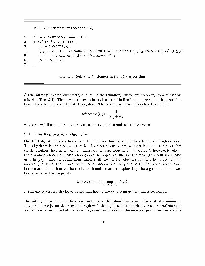
5.3 Selecting Customers to Relocate

The LNS algorithm uses the same strategy as in [28] to select the customers to relocate. Theimplementation is depicted in Figure 4. It �rst selects a customer randomly (line 1) and iterateslines 3-6 to remove the n � 1 remaining customers. Each such iteration selects a customer from

10

Function SelectCustomers(�,n)

1. S := f random(Customers) g;2. for(i := 2;i � n; i++) f3. c := random(S);4. hc0; : : : ; cN�ii := Customers n S such that relateness(c; ci) � relateness(c; cj) (i � j);5. r := := brandom([0; 1])� � jCustomers n Sjc;6. S := S [ fcrg;7. g

Figure 4: Selecting Customers in the LNS Algorithm

S (the already selected customers) and ranks the remaining customers according to a relatenesscriterion (lines 3-4). The new customer to insert is selected in line 5 and, once again, the algorithmbiases the selection toward related neighbors. The relateness measure is de�ned as in [28]:

relateness(i; j) =1

c0ij + vij

where vij = 1 if customers i and j are on the same route and is zero otherwise.

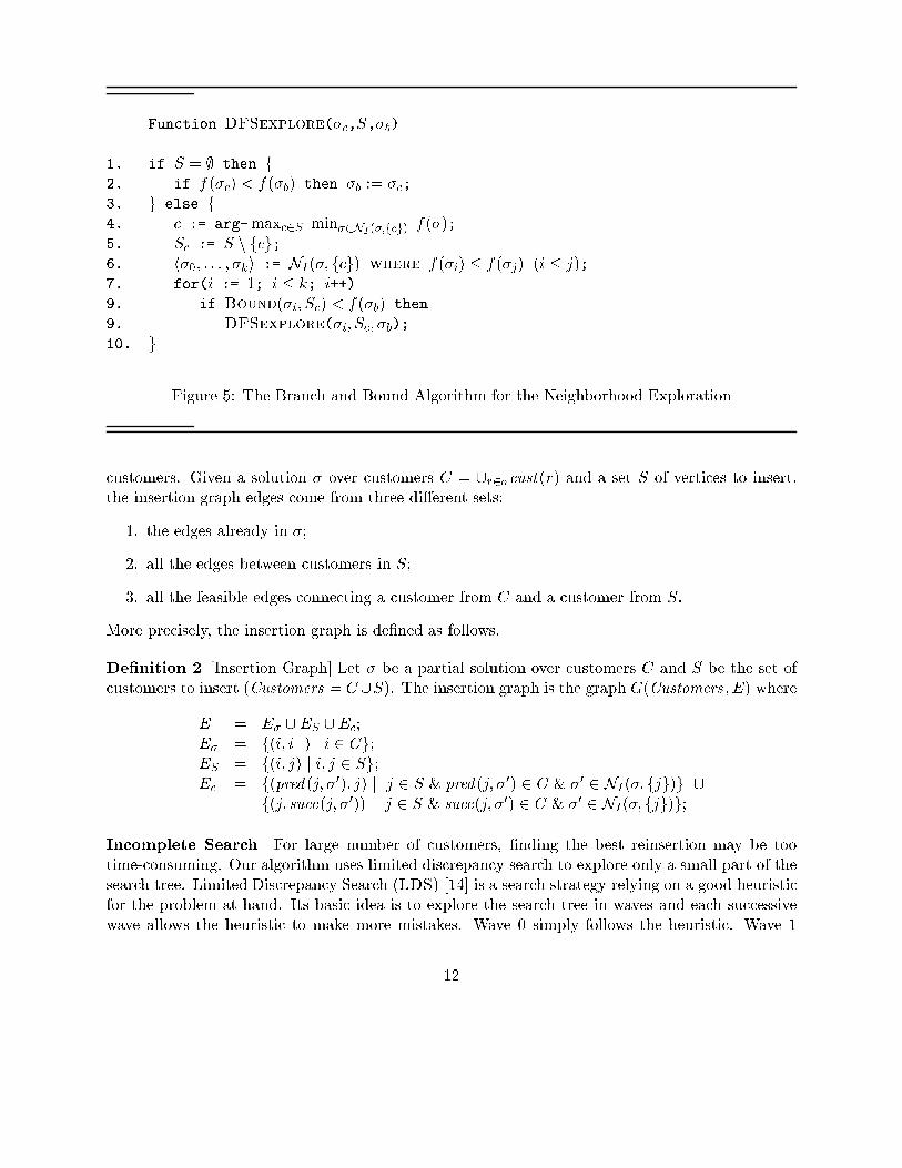
5.4 The Exploration Algorithm

Our LNS algorithm uses a branch and bound algorithm to explore the selected subneighborhood.The algorithm is depicted in Figure 5. If the set of customers to insert is empty, the algorithmchecks whether the current solution improves the best solution found so far. Otherwise, it selectsthe customer whose best insertion degrades the objective function the most (this heuristic is alsoused in [28]). The algorithm then explores all the partial solutions obtained by inserting c byincreasing order of their travel costs. Also, observe that only the partial solutions whose lowerbounds are better than the best solution found so far are explored by the algorithm. The lowerbound satis�es the inequality

Bound(�; S) � min�02NI(�;S)

f(�0):

It remains to discuss the lower bound and how to keep the computation times reasonable.

Bounding The bounding function used in the LNS algorithm returns the cost of a minimumspanning k-tree [8] on the insertion graph with the depot as distinguished vertex, generalizing thewell-known 1-tree bound of the travelling salesman problem. The insertion graph vertices are the

11

Function DFSexplore(�c,S,�b)

1. if S = ; then f2. if f(�c) < f(�b) then �b := �c;3. g else f4. c := arg-maxc2S min�2NI(�;fcg) f(�);

5. Sc := S n fcg;6. h�0; : : : ; �ki := NI(�; fcg) where f(�i) � f(�j) (i � j);7. for(i := 1; i � k; i++)9. if Bound(�i; Sc) < f(�b) then

9. DFSexplore(�i; Sc; �b);10. g

Figure 5: The Branch and Bound Algorithm for the Neighborhood Exploration

customers. Given a solution � over customers C = [r2�cust(r) and a set S of vertices to insert,the insertion graph edges come from three di�erent sets:

1. the edges already in �;

2. all the edges between customers in S;

3. all the feasible edges connecting a customer from C and a customer from S.

More precisely, the insertion graph is de�ned as follows.

De�nition 2 [Insertion Graph] Let � be a partial solution over customers C and S be the set ofcustomers to insert (Customers = C[S). The insertion graph is the graph G(Customers ; E) where

E = E� [ES [Ec;E� = f(i; i+) j i 2 Cg;ES = f(i; j) j i; j 2 Sg;Ec = f(pred (j; �0); j) j j 2 S & pred (j; �0) 2 C & �0 2 NI(�; fjg)g [

f(j; succ(j; �0)) j j 2 S & succ(j; �0) 2 C & �0 2 NI(�; fjg)g;

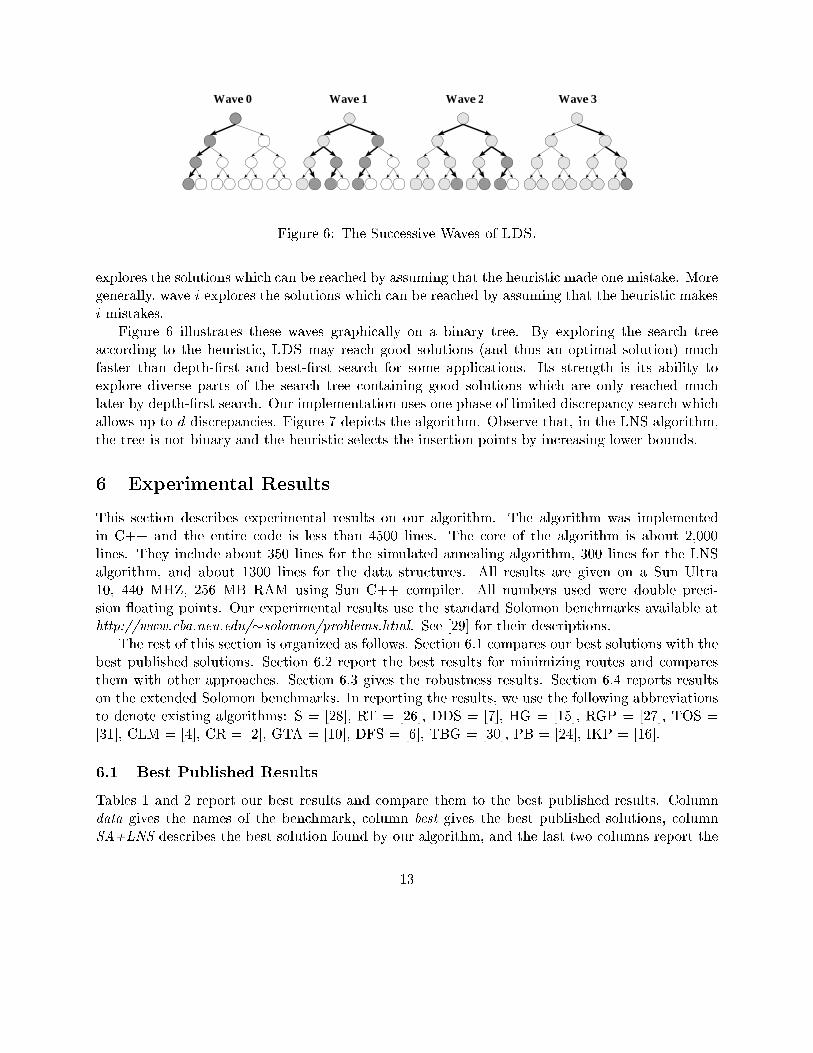
Incomplete Search For large number of customers, �nding the best reinsertion may be tootime-consuming. Our algorithm uses limited discrepancy search to explore only a small part of thesearch tree. Limited Discrepancy Search (LDS) [14] is a search strategy relying on a good heuristicfor the problem at hand. Its basic idea is to explore the search tree in waves and each successivewave allows the heuristic to make more mistakes. Wave 0 simply follows the heuristic. Wave 1

12

Wave 0 Wave 1 Wave 2 Wave 3

Figure 6: The Successive Waves of LDS.

explores the solutions which can be reached by assuming that the heuristic made one mistake. Moregenerally, wave i explores the solutions which can be reached by assuming that the heuristic makesi mistakes.

Figure 6 illustrates these waves graphically on a binary tree. By exploring the search treeaccording to the heuristic, LDS may reach good solutions (and thus an optimal solution) muchfaster than depth-�rst and best-�rst search for some applications. Its strength is its ability toexplore diverse parts of the search tree containing good solutions which are only reached muchlater by depth-�rst search. Our implementation uses one phase of limited discrepancy search whichallows up to d discrepancies. Figure 7 depicts the algorithm. Observe that, in the LNS algorithm,the tree is not binary and the heuristic selects the insertion points by increasing lower bounds.

6 Experimental Results

This section describes experimental results on our algorithm. The algorithm was implementedin C++ and the entire code is less than 4500 lines. The core of the algorithm is about 2,000lines. They include about 350 lines for the simulated annealing algorithm, 300 lines for the LNSalgorithm, and about 1300 lines for the data structures. All results are given on a Sun Ultra10, 440 MHZ, 256 MB RAM using Sun C++ compiler. All numbers used were double preci-sion oating points. Our experimental results use the standard Solomon benchmarks available athttp://www.cba.neu.edu/�solomon/problems.html. See [29] for their descriptions.

The rest of this section is organized as follows. Section 6.1 compares our best solutions with thebest published solutions. Section 6.2 report the best results for minimizing routes and comparesthem with other approaches. Section 6.3 gives the robustness results. Section 6.4 reports resultson the extended Solomon benchmarks. In reporting the results, we use the following abbreviationsto denote existing algorithms: S = [28], RT = [26], DDS = [7], HG = [15], RGP = [27], TOS =[31], CLM = [4], CR = [2], GTA = [10], DFS = [6], TBG = [30], PB = [24], IKP = [16].

6.1 Best Published Results

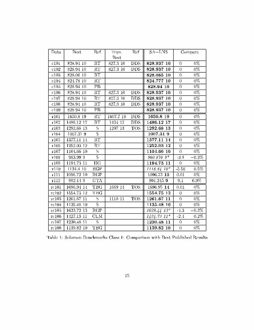
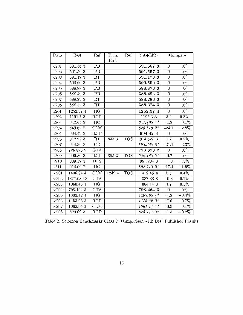
Tables 1 and 2 report our best results and compare them to the best published results. Columndata gives the names of the benchmark, column best gives the best published solutions, columnSA+LNS describes the best solution found by our algorithm, and the last two columns report the

13

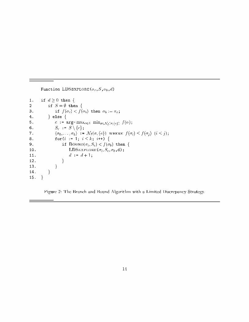
Function LDSexplore(�c,S,�b,d)

1. if d � 0 then f2 if S = ; then f3. if f(�c) < f(�b) then �b := �c;4. g else f5. c := arg-maxc2S min�2NI (�;fcg) f(�);

6. Sc := S n fcg;7. h�0; : : : ; �ki := NI(�; fcg) where f(�i) � f(�j) (i � j);8. for(i := 1; i � k; i++) f9. if Bound(�i; Sc) < f(�b) then f10. LDSexplore(�i; Sc; �b,d);11. d := d+ 1;12. g13. g14. g15. g

Figure 7: The Branch and Bound Algorithm with a Limited Discrepancy Strategy.

14

Data Best Ref Trun. Ref SA+LNS CompareBest

c101 828.94 10 RT 827.3 10 DDS 828.937 10 0 0%

c102 828.94 10 RT 827.3 10 DDS 828.937 10 0 0%

c103 828.06 10 RT 828.065 10 0 0%

c104 824.78 10 RT 824.777 10 0 0%

c105 828.94 10 PB 828.94 10 0 0%

c106 828.94 10 RT 827.3 10 DDS 828.937 10 0 0%

c107 828.94 10 RT 827.3 10 DDS 828.937 10 0 0%

c108 828.94 10 RT 827.3 10 DDS 828.937 10 0 0%

c109 828.94 10 PB 828.937 10 0 0%

r101 1650.8 19 RT 1607.7 18 DDS 1650.8 19 0 0%

r102 1486.12 17 RT 1434 17 DDS 1486.12 17 0 0%

r103 1292.68 13 S 1207 13 TOS 1292.68 13 0 0%

r104 1007.31 9 S 1007.31 9 0 0%

r105 1377.11 14 RT 1377.11 14 0 0%

r106 1252.03 12 RT 1252.03 12 0 0%

r107 1104.66 10 S 1104.66 10 0 0%

r108 963.99 9 S 960.876 9* -3.1 �0:3%r109 1194.73 11 HG 1194.73 11 0 0%

r110 1124.4 10 RGP 1118.84 10* -5.56 �0:5%r111 1096.72 10 RGP 1096.73 10 0.01 0%

r112 982.14 9 GTA 991.245 9 9.1 0:9%

rc101 1696.94 14 TBG 1669 14 TOS 1696.95 14 0.01 0%

rc102 1554.75 12 TBG 1554.75 12 0 0%

rc103 1261.67 11 S 1110 11 TOS 1261.67 11 0 0%

rc104 1135.48 10 S 1135.48 10 0 0%

rc105 1633.72 13 RGP 1629.44 13* -4.3 �0:3%rc106 1427.13 11 CLM 1424.73 11* -2.4 �0:2%rc107 1230.48 11 S 1230.48 11 0 0%

rc108 1139.82 10 TBG 1139.82 10 0 0%

Table 1: Solomon Benchmarks Class 1: Comparison with Best Published Results

15

Data Best Ref Trun. Ref SA+LNS CompareBest

c201 591.56 3 PB 591.557 3 0 0%

c202 591.56 3 PB 591.557 3 0 0%

c203 591.17 3 RT 591.173 3 0 0%

c204 590.60 3 PB 590.599 3 0 0%

c205 588.88 3 PB 588.876 3 0 0%

c206 588.49 3 PB 588.493 3 0 0%

c207 588.29 3 RT 588.286 3 0 0%

c208 588.32 3 RT 588.324 3 0 0%

r201 1252.37 4 HG 1252.37 4 0 0%

r202 1191.7 3 RGP 1195.3 3 3.6 0:3%

r203 942.64 3 HG 941.408 3* -1.2 �0:1%r204 849.62 2 CLM 825.519 2* -24.1 �2:8%r205 994.42 3 RGP 994.42 3 0 0%

r206 912.97 3 RT 833 3 TOS 914.627 3 1.7 0:2%

r207 914.39 2 CR 893.328 2* -21.1 �2:3%r208 726.823 2 GTA 726.823 2 0 0%

r209 909.86 3 RGP 855 3 TOS 909.163 3* -0.7 0%

r210 939.37 3 DFS 951.294 3 11.9 1:3%

r211 910.09 2 HG 892.713 2* -17.4 �1:9%

rc201 1406.94 4 CLM 1249 4 TOS 1412.45 4 5.5 0:4%

rc202 1377.089 3 GTA 1387.38 3 10.3 0:7%

rc203 1060.45 3 HG 1064.14 3 3.7 0:3%

rc204 798.464 3 GTA 798.464 3 0 0%

rc205 1302.42 4 HG 1297.65 4* -4.8 �0:4%rc206 1153.93 3 RGP 1146.32 3* -7.6 �0:7%rc207 1062.05 3 CLM 1061.14 3* -0.9 �0:1%rc208 829.69 3 RGP 828.141 3* -1.5 �0:2%

Table 2: Solomon Benchmarks Class 2: Comparison with Best Published Results

16

Data RT TBG CR CLM HG DFS GTA S SA+LNS

c1 10 10 10 10 10 10 10 10 10

c2 3 3 3 3 3 3 3 - 3

r1 12.25 12.17 12.17 12.08 11.92 12.5 12 12 11.92

r2 2.91 2.82 2.73 2.73 2.73 3 2.73 - 2.73

rc1 11.88 11.5 11.88 11.5 11.5 12 11.63 11.75 11.5

rc2 3.38 3.38 3.25 3.25 3.25 3.38 3.25 - 3.25

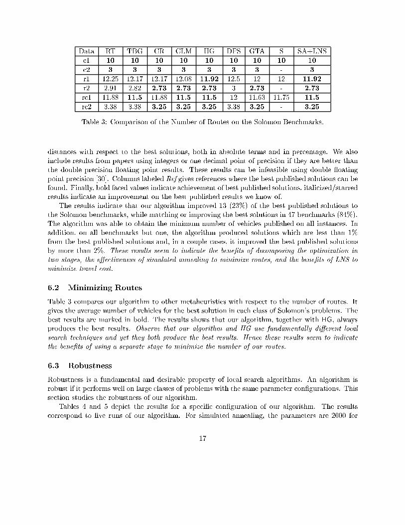
Table 3: Comparison of the Number of Routes on the Solomon Benchmarks.

distances with respect to the best solutions, both in absolute terms and in percentage. We alsoinclude results from papers using integers or one decimal point of precision if they are better thanthe double precision oating point results. These results can be infeasible using double oatingpoint precision [30]. Columns labeled Ref gives references where the best published solutions can befound. Finally, bold faced values indicate achievement of best published solutions, italicized/starredresults indicate an improvement on the best published results we know of.

The results indicate that our algorithm improved 13 (23%) of the best published solutions tothe Solomon benchmarks, while matching or improving the best solutions in 47 benchmarks (84%).The algorithm was able to obtain the minimum number of vehicles published on all instances. Inaddition, on all benchmarks but one, the algorithm produced solutions which are less than 1%from the best published solutions and, in a couple cases, it improved the best published solutionsby more than 2%. These results seem to indicate the bene�ts of decomposing the optimization intwo stages, the e�ectiveness of simulated annealing to minimize routes, and the bene�ts of LNS tominimize travel cost.

6.2 Minimizing Routes

Table 3 compares our algorithm to other metaheuristics with respect to the number of routes. Itgives the average number of vehicles for the best solution in each class of Solomon's problems. Thebest results are marked in bold. The results shows that our algorithm, together with HG, alwaysproduces the best results. Observe that our algorithm and HG use fundamentally di�erent localsearch techniques and yet they both produce the best results. Hence these results seem to indicatethe bene�ts of using a separate stage to minimize the number of our routes.

6.3 Robustness

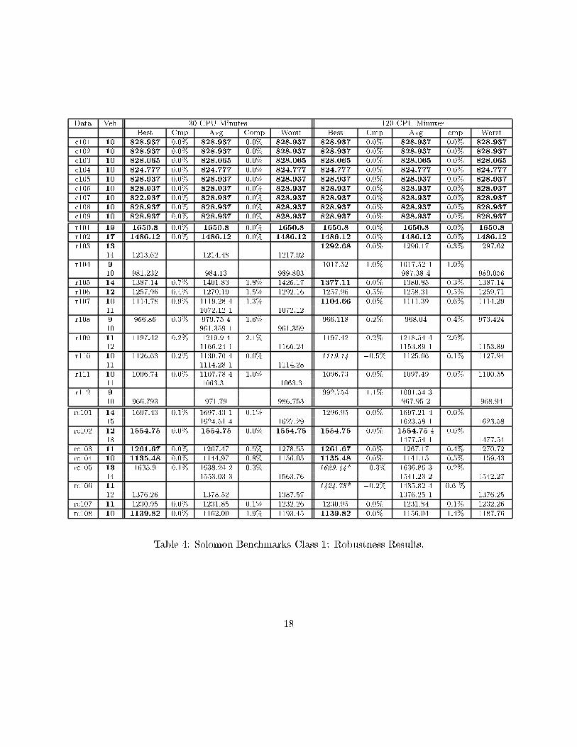
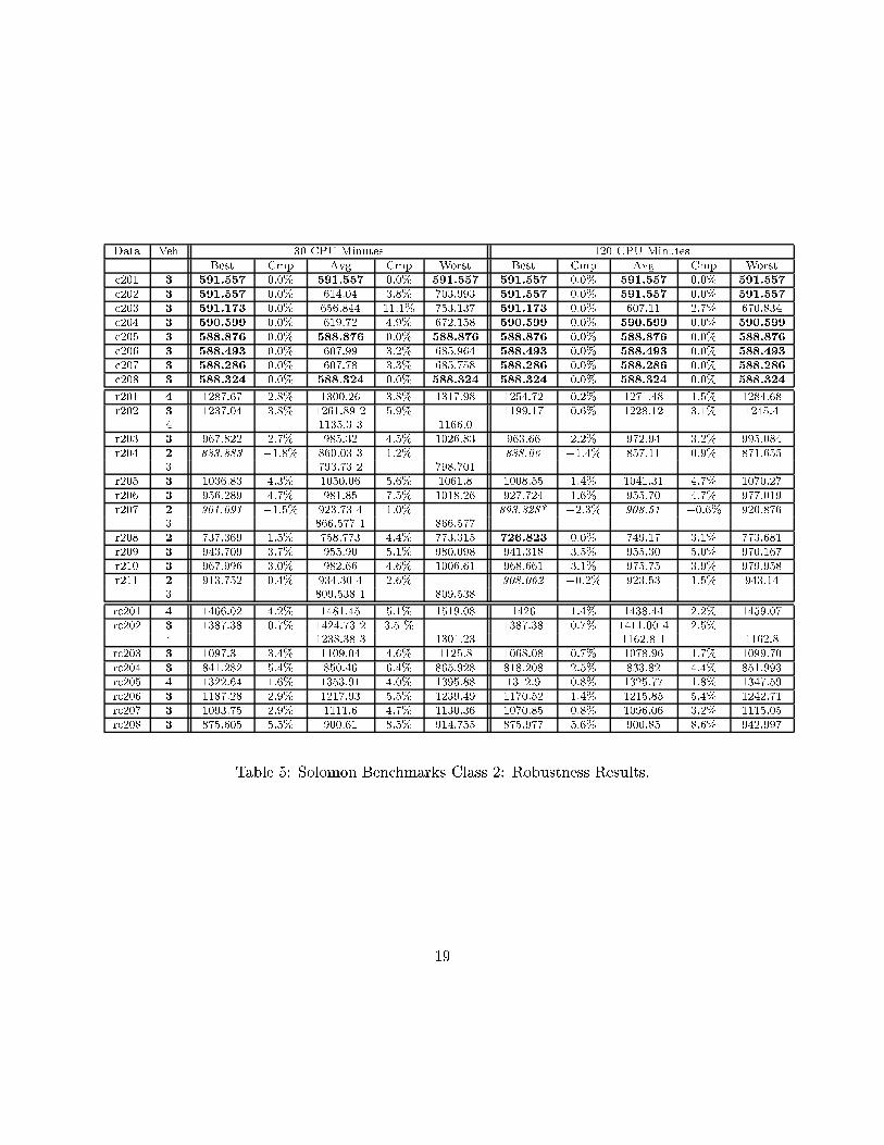
Robustness is a fundamental and desirable property of local search algorithms. An algorithm isrobust if it performs well on large classes of problems with the same parameter con�gurations. Thissection studies the robustness of our algorithm.

Tables 4 and 5 depict the results for a speci�c con�guration of our algorithm. The resultscorrespond to �ve runs of our algorithm. For simulated annealing, the parameters are 2000 for

17

Data Veh 30 CPU Minutes 120 CPU MinutesBest Cmp Avg Comp Worst Best Cmp Avg cmp Worst

c101 10 828.937 0:0% 828.937 0:0% 828.937 828.937 0:0% 828.937 0:0% 828.937

c102 10 828.937 0:0% 828.937 0:0% 828.937 828.937 0:0% 828.937 0:0% 828.937

c103 10 828.065 0:0% 828.065 0:0% 828.065 828.065 0:0% 828.065 0:0% 828.065

c104 10 824.777 0:0% 824.777 0:0% 824.777 824.777 0:0% 824.777 0:0% 824.777

c105 10 828.937 0:0% 828.937 0:0% 828.937 828.937 0:0% 828.937 0:0% 828.937

c106 10 828.937 0:0% 828.937 0:0% 828.937 828.937 0:0% 828.937 0:0% 828.937

c107 10 822.937 0:0% 828.937 0:0% 828.937 828.937 0:0% 828.937 0:0% 828.937

c108 10 828.937 0:0% 828.937 0:0% 828.937 828.937 0:0% 828.937 0:0% 828.937

c109 10 828.937 0:0% 828.937 0:0% 828.937 828.937 0:0% 828.937 0:0% 828.937

r101 19 1650.8 0:0% 1650.8 0:0% 1650.8 1650.8 0:0% 1650.8 0:0% 1650.8

r102 17 1486.12 0:0% 1486.12 0:0% 1486.12 1486.12 0:0% 1486.12 0:0% 1486.12

r103 13 1292.68 0:0% 1296.17 0:3% 1297.6214 1213.62 1214.48 1217.92

r104 9 1017.52 1:0% 1017.52 1 1.0%10 981.232 984.13 989.803 987.38 4 989.056

r105 14 1387.14 0:7% 1401.83 1:8% 1426.17 1377.11 0:0% 1380.85 0:3% 1387.14r106 12 1257.96 0:4% 1270.19 1:5% 1292.16 1257.96 0:5% 1258.31 0:5% 1259.71r107 10 1114.78 0:9% 1119.28 4 1.3% 1104.66 0:0% 1111.39 0:6% 1114.29

11 1072.12 1 1072.12r108 9 966.86 0:3% 979.75 4 1.6% 966.118 0:2% 968.04 0:4% 973.424

10 961.359 1 961.359r109 11 1197.42 0:2% 1219.9 4 2.1% 1197.42 0:2% 1218.54 4 2.0%

12 1166.24 1 1166.24 1153.89 1 1153.89r110 10 1126.63 0:2% 1130.76 4 0.6% 1119.14 �0:5% 1125.66 0:1% 1127.94

11 1114.28 1 1114.28r111 10 1096.74 0:0% 1107.78 4 1.0% 1096.73 0:0% 1097.49 0:0% 1100.55

11 1063.3 1 1063.3r112 9 992.754 1:1% 1001.54 3

10 966.793 971.79 986.753 967.95 2 968.94

rc101 14 1697.43 0:1% 1697.43 1 0.1% 1296.95 0:0% 1697.21 4 0.0%15 1624.51 4 1627.29 1623.58 1 1623.58

rc102 12 1554.75 0:0% 1554.75 0:0% 1554.75 1554.75 0:0% 1554.75 4 0.0%13 1477.54 1 1477.54

rc103 11 1261.67 0:0% 1267.47 0:5% 1278.55 1261.67 0:0% 1267.17 0:4% 1270.72rc104 10 1135.48 0:0% 1144.97 0:8% 1156.05 1135.48 0:0% 1141.15 0:5% 1159.43rc105 13 1635.9 0:1% 1638.24 2 0.3% 1629.44* �0:3% 1636.86 3 0.2%

14 1553.03 3 1563.76 1541.23 2 1542.27rc106 11 1424.73* �0:2% 1435.82 4 0.6 %

12 1376.26 1378.52 1387.57 1376.25 1 1376.25rc107 11 1230.95 0:0% 1231.85 0:1% 1232.26 1230.95 0:0% 1231.84 0:1% 1232.26rc108 10 1139.82 0:0% 1162.00 1:9% 1193.45 1139.82 0:0% 1156.04 1:4% 1187.76

Table 4: Solomon Benchmarks Class 1: Robustness Results.

18

Data Veh 30 CPU Minutes 120 CPU MinutesBest Cmp Avg Cmp Worst Best Cmp Avg Cmp Worst

c201 3 591.557 0:0% 591.557 0:0% 591.557 591.557 0:0% 591.557 0:0% 591.557

c202 3 591.557 0:0% 614.04 3:8% 703.993 591.557 0:0% 591.557 0:0% 591.557

c203 3 591.173 0:0% 656.844 11:1% 753.137 591.173 0:0% 607.11 2:7% 670.834c204 3 590.599 0:0% 619.72 4:9% 672.158 590.599 0:0% 590.599 0:0% 590.599

c205 3 588.876 0:0% 588.876 0:0% 588.876 588.876 0:0% 588.876 0:0% 588.876

c206 3 588.493 0:0% 607.99 3:2% 685.964 588.493 0:0% 588.493 0:0% 588.493

c207 3 588.286 0:0% 607.78 3:3% 685.758 588.286 0:0% 588.286 0:0% 588.286

c208 3 588.324 0:0% 588.324 0:0% 588.324 588.324 0:0% 588.324 0:0% 588.324

r201 4 1287.67 2:8% 1300.26 3:8% 1317.98 1254.72 0:2% 1271.48 1:5% 1284.68r202 3 1237.04 3:8% 1261.89 2 5.9% 1199.17 0:6% 1228.12 3:1% 1245.4

4 1135.3 3 1166.0r203 3 967.822 2:7% 985.32 4:5% 1026.83 963.66 2:2% 972.94 3:2% 995.084r204 2 833.883 �1:8% 860.03 3 1.2% 838.06 �1:4% 857.11 0:9% 871.655

3 793.73 2 798.701r205 3 1036.83 4:3% 1050.06 5:6% 1061.8 1008.55 1:4% 1041.31 4:7% 1070.27r206 3 956.289 4:7% 981.85 7:5% 1018.26 927.724 1:6% 955.70 4:7% 977.019r207 2 901.091 �1:5% 923.73 4 1.0% 893.328* �2:3% 908.51 �0:6% 920.876

3 866.577 1 866.577r208 2 737.369 1:5% 758.773 4:4% 773.315 726.823 0:0% 749.17 3:1% 773.681r209 3 943.709 3:7% 955.90 5:1% 980.098 941.318 3:5% 955.30 5:0% 970.167r210 3 967.996 3:0% 982.66 4:6% 1006.61 968.661 3:1% 975.75 3:9% 979.958r211 2 913.752 0:4% 934.30 4 2.6% 908.062 �0:2% 923.53 1:5% 943.14

3 809.538 1 809.538

rc201 4 1466.02 4:2% 1481.45 5:1% 1519.08 1426 1:4% 1438.44 2:2% 1459.07rc202 3 1387.38 0:7% 1424.73 2 3.5 % 1387.38 0:7% 1411.00 4 2.5%

4 1238.38 3 1301.23 1162.8 1 1162.8rc203 3 1097.31 3:4% 1109.04 4:6% 1125.8 1068.08 0:7% 1078.96 1:7% 1099.70rc204 3 841.282 5:4% 850.46 6:4% 865.928 818.208 2:5% 833.82 4:4% 851.993rc205 4 1322.64 1:6% 1353.91 4:0% 1395.88 1312.9 0:8% 1325.77 1:8% 1347.59rc206 3 1187.28 2:9% 1217.93 5:5% 1239.49 1170.52 1:4% 1215.85 5:4% 1242.71rc207 3 1093.75 2:9% 1111.6 4:7% 1130.36 1070.85 0:8% 1096.06 3:2% 1115.05rc208 3 875.605 5:5% 900.61 8:5% 914.755 875.977 5:6% 900.85 8:6% 942.997

Table 5: Solomon Benchmarks Class 2: Robustness Results.

19

Data RT TBG GTA S SA+LNS SA+LNS SA+LNS SA+LNS Best1800 3600 1800 3600 5400 7200 Possible

c1 10 10 10 - 10 10 10 10 10540 2926

c2 3 3 3 - 3 3 3 3 31200 3275

r1 12.58 12.33 12.38 12.33 12.25 12.2 12.07 12.03 11.921300 13774

r2 3.09 3.00 3.00 - 2.85 2.76 2.75 2.73 2.734900 3372

rc1 12.38 11.9 11.92 11.95 11.8 11.7 11.65 11.63 11.52600 11264

rc2 3.62 3.38 3.33 - 3.3 3.35 3.33 3.28 3.251300 1933

Table 6: Solomon Benchmarks: Robustness of the Route Minimization.

starting temperature, .95 for cooling factor �, 2500 iterations per each temperature, .01 minimumtemperature, 10 for the simulated annealing determinism factor �. For LNS, the parameters are35 for the maximum customers to remove p, 1000 iterations w/o improvement before removing onemore customers, 15 for the determinism factor � and 4 discrepancies. The allowed time is split 1

3 forSA and 2

3 for LNS. Bold-faced numbers indicate matches with the best published results. Italicizednumbers indicate results better than the best published solutions. Italicized and starred numbersindicate results better than the best published solutions and equal to best results we found. Wheredi�erent numbers of vehicles were discovered, the number of times each vehicle result is obtained isindicated next to the average results. There are a number of interesting observations to be drawnfrom these results.

Best Results The algorithm �nds the best published result (or an improvement thereof) inall 5 runs in 15 problems (27%) after 30 minutes and in 18 problems (32%) after 120 minutes.Furthermore, the best published result (or an improvement thereof) is achieved at least once in 24problems (43%) after 30 minutes and in 33 problems after 120 minutes (59%). In the 30 minutesruns, the algorithm improves the best published results in two cases with the standard con�gurationand it is almost always within 5% of the best published solutions. In the 120 minutes runs, thealgorithm improves the best published results in six cases with the standard con�guration and isalways within 3.5% of the best published solutions except in one case (5.6%). In general, givingmore time to the algorithm helps produce better solutions, although this is not always true (sincesimulated annealing gives extremely random starting solutions).

20

Average Results The average results are harder to compare systematically since all �ve runsdo not always produce the best number of routes. However, it can be seen that they are neververy far from the best solutions. For the 30 minutes runs, they are in general within 2% of thebest solutions on class 1 and within 6% on class 2. For the 120 minutes runs, they are alwayswithin 2% and almost always within 1% on class 1 and almost always within 5% on class 2. It isalso interesting to compare the average results in 120 minutes and the best results in 30 minutes.These results are in fact quite similar in quality, which is a good indication of the robustness of thealgorithm.

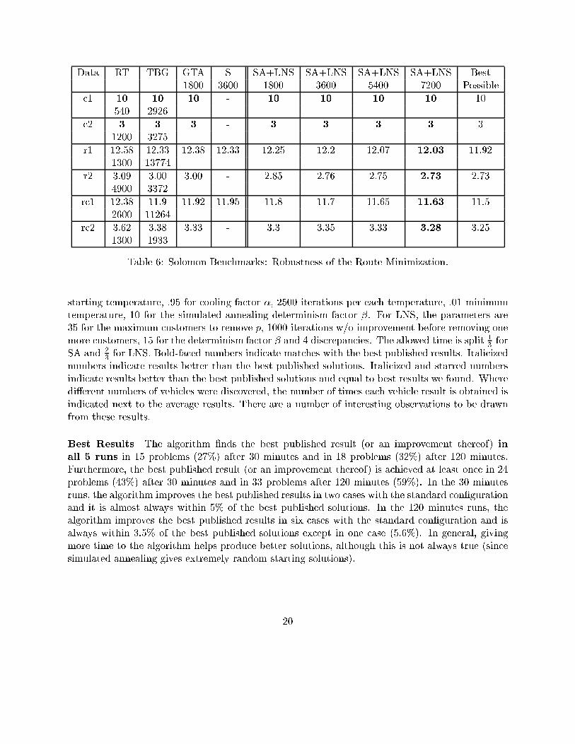
Route Minimization Table 6 reports the average number of vehicles required over 5 runs andcompares these results with other approaches where the papers gave averages across independentruns of their programs. The results are clustered by problem classes. The best results are in bold.CPU time is given in the column headers or underneath the results. Note, however, that comparingtimes is misleading as prior results were achieved on less powerful machines. The �nal column givesthe best possible value for each class, i.e., the average number of vehicles for the class if the bestpublished number of vehicles is achieved for each benchmark.

Observe that, after 30 minutes, our algorithm beats the average number of vehicles of anypublished results using this metric. On the non-trivial r2 class, our algorithm achieves the bestpossible value inferred from the published results. Once again, the results indicate the robustnessof our algorithm.

Summary Overall, the algorithm appears to be very robust, performing well on all instances ofthe benchmarks. The algorithm is robust both with respect to route minimization and travel costminimization on these benchmarks. This is one of the strengths of the algorithm, together with itsability to produce excellent solutions on all benchmarks.

6.4 Extended Solomon Benchmarks

Table 7 and 8 contain our best results for the extended solomon benchmark problems. To thebest of our knowledge, there are no results to compare our algorithm to, except for some minimumnumber of vehicle results. Results are rounded to 6 signi�cant digits. The only results we knowon these problems are from [16] and concern only the number of vehicles. They are given in thecolumn labeled IKP.

7 Discussion and Related Work

This paper presented a two stage hybrid local search algorithm for the vehicle routing problemwith time windows. To our knowledge, reference [15] is the only other paper presenting a two stagealgorithm for vehicle routing. Their algorithm is not hybrid however and uses the same evolutionarymetaheuristic with two evaluation functions. Their evolutionary metaheuristic uses the uniformorder-based crossover of [5] and their mutation operators are or-opt from [22] (generalized so thatsequences of customers can be moved to other vehicles), �-interchange [23], and 2-opt* from [25].

21

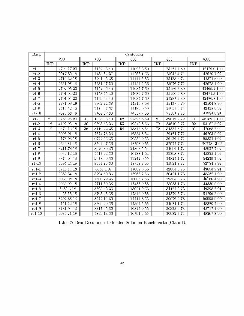
Data Customers200 400 600 800 1000

IKP IKP IKP IKP IKPc1-1 2704.57 20 7152.06 40 14095.6 60 25184.4 80 42479.0 100c1-2 2917.89 18 7435.84 37 15266.1 56 25947.4 75 42920.7 92c1-3 2719.62 18 7291.45 36 14414.5 56 25438.6 72 42571.6 90c1-4 2651.98 18 7231.07 36 14454.2 56 25076.7 72 42678.1 90c1-5 2702.05 20 7152.06 40 14085.7 60 25166.3 80 42469.2 100c1-6 2701.04 20 7153.45 40 14089.7 60 25160.9 80 42471.3 100c1-7 2701.04 20 7149.43 40 14085.7 60 25287.9 80 42486.8 100c1-8 2781.09 19 7302.24 38 14346.8 58 25437.0 76 42564.8 96c1-9 2716.42 18 7173.37 37 14180.6 56 25655.6 73 42428.0 92c1-10 2670.63 18 7168.62 36 14552.2 56 25561.9 73 41984.0 91

r1-1 21 4785.96 20 41 10536.5 40 62 22393.8 59 81 39612.2 79 101 58169.5 100r1-2 18 4102.03 18 36 9308.53 36 55 19319.6 55 72 34610.9 72 92 53167.5 92r1-3 18 3473.53 18 36 8119.22 36 54 18812.8 54 72 31534.8 72 91 47668.2 92r1-4 3096.91 18 7674.75 36 16854.8 54 29481.7 72 46203.0 92r1-5 4173.93 18 9722.66 36 20550.9 55 36139.4 72 55531.4 92r1-6 3634.81 18 8594.27 36 18798.0 55 32975.7 72 50778. 3 92r1-7 3211,78 18 8026.80 36 21868.5 54 31009.1 72 48037.7 92r1-8 3032.12 18 7517.22 36 16488.1 54 29268.8 72 45355.1 92r1-9 3874.04 18 9078.99 36 19242.0 55 34824.7 72 54239.3 92r1-10 3394.44 18 8554.75 36 18757.7 55 33921.8 72 52784.7 92

rc1-1 3748.24 18 8834.4 37 17682.0 56 32003.5 73 49658.9 91rc1-2 3382.34 18 8294.59 36 16963.2 55 30421.1 73 48537.1 90rc1-3 3066.08 18 7800.79 36 16008.7 55 29305.0 73 46760.4 90rc1-4 2939.02 18 7711.69 36 15455.0 55 28035.1 73 44330.0 90rc1-5 3489.6 18 8805.42 36 18021.0 55 31484.0 73 49398.2 91rc1-6 3465.55 18 8705.25 36 17812.9 55 31579.5 73 51296.2 90rc1-7 3292.33 18 8572.14 36 17444.3 55 30676.9 73 50995.0 90rc1-8 3151.62 18 8369.29 36 17364.5 55 31081.1 73 48380.5 90rc1-9 3181.94 18 8317.05 36 16815.9 55 30333.0 73 48717.4 90rc1-10 3083.21 18 7899.18 36 16791.6 55 30082.3 73 48267.8 90

Table 7: Best Results on Extended Solomon Benchmarks (Class 1).

22

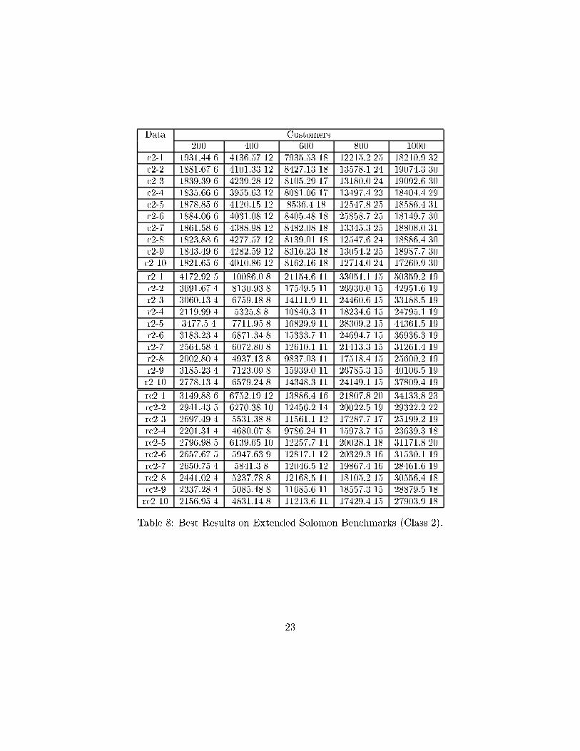
Data Customers200 400 600 800 1000

c2-1 1931.44 6 4136.57 12 7935.53 18 12215.2 25 18210.9 32c2-2 1881.67 6 4101.33 12 8427.13 18 13578.1 24 19074.3 30c2-3 1839.39 6 4239.28 12 8105.29 17 13180.0 24 19092.6 30c2-4 1835.66 6 3955.63 12 8081.06 17 13497.4 23 18404.4 29c2-5 1878.85 6 4120.15 12 8536.4 18 12547.8 25 18586.4 31c2-6 1884.06 6 4031.08 12 8405.48 18 25858.7 25 18149.7 30c2-7 1861.58 6 4388.98 12 8482.08 18 13345.3 25 18808.0 31c2-8 1823.88 6 4277.57 12 8139.01 18 12547.6 24 18886.4 30c2-9 1843.49 6 4282.59 12 8316.23 18 13054.2 25 18987.7 30c2-10 1821.65 6 4010.86 12 8162.16 18 12714.0 24 17260.9 30

r2-1 4172.92 5 10086.0 8 21154.6 11 33051.1 15 50359.2 19r2-2 3691.67 4 8130.93 8 17549.5 11 26930.0 15 42951.6 19r2-3 3060.13 4 6759.18 8 14111.9 11 24460.6 15 33188.5 19r2-4 2119.99 4 5325.8 8 10840.3 11 18234.6 15 24795.1 19r2-5 3477.5 4 7711.95 8 16829.9 11 28309.2 15 44361.5 19r2-6 3183.23 4 6871.34 8 15333.7 11 24694.7 15 36936.3 19r2-7 2564.58 4 6072.80 8 12610.1 11 21413.3 15 31261.4 19r2-8 2002.80 4 4937.13 8 9837.03 11 17518.4 15 25600.2 19r2-9 3185.23 4 7123.09 8 15939.0 11 26785.3 15 40106.5 19r2-10 2778.13 4 6579.24 8 14348.3 11 24149.1 15 37809.4 19

rc2-1 3149.88 6 6752.19 12 13886.4 16 21807.8 20 34133.8 23rc2-2 2941.43 5 6270.38 10 12456.2 14 20022.5 19 29322.2 22rc2-3 2697.49 4 5531.38 8 11561.1 12 17287.7 17 25199.2 19rc2-4 2201.31 4 4680.07 8 9786.24 11 15973.7 15 23639.3 18rc2-5 2796.98 5 6139.65 10 12257.7 14 20028.1 18 31171.8 20rc2-6 2657.67 5 5947.63 9 12817.1 12 20329.3 16 31530.1 19rc2-7 2650.75 4 5841.3 8 12046.5 12 19867.4 16 28461.6 19rc2-8 2441.02 4 5237.78 8 12168.5 11 18105.2 15 30556.4 18rc2-9 2337.28 4 5085.48 8 11685.6 11 18557.3 15 28879.5 18rc2-10 2156.95 4 4831.14 8 11213.6 11 17429.4 15 27903.9 18

Table 8: Best Results on Extended Solomon Benchmarks (Class 2).

23

Their evaluation function to minimize routes is a lexicographic function with three components.Their second component is the size of the smallest route, while ours is the sum of the squares of theroute sizes. Their third component is the minimal delay of the routing plan. Their motivation forusing a two-stage algorithm is similar to ours: the recognition that minimizing travel costs may notalways be most e�ective for minimizing the number of routes. One of the contributions of this paperis to provide evidence of the bene�ts of a two-stage approach for vehicle routing with time windows.Indeed, the fundamentally di�erent nature of these two two-stage algorithms, together with theire�ectiveness, seem to indicate that the two-stage approach has bene�ts across metaheuristics.

The �rst stage of our algorithm uses a novel simulated annealing algorithm. The algorithm usestraditional moves operators described in [6, 18]: 2-exchange, Or-exchange, relocation, crossover,and exchange. A critical aspect of the simulated annealing is the lexicographic evaluation function.Its second component, maximizing the sum of the squares of route sizes, was inspired by somegraph-coloring algorithms [17]. Its third component is the minimal delay of [15]. Our simulatedannealing algorithm also includes some greedy components typical of tabu search [12], includingan aspiration criterion and a bias towards good solutions in the random process. These greedyaspects were shown to be bene�cial experimentally. Of course, simulated annealing was used forsolving vehicle routing problems in the past. In particular, reference [1] describes a simulatedannealing where the neighborhood is de�ned by the �-interchange mechanism of [23] and the k-node interchange mechanism of [3]. The algorithm in [1] makes use of a tabu list within thesimulated annealing process and uses a weighted objective function incorporating total time alongwith number of vehicles and travel cost. Probably the main contribution here is the novel evaluationfunction and the additional evidence that minimal delay is a fundamental concept in minimizingthe number routes.

The second stage of our algorithm uses the LNS technique pioneered by [28]. In that paper,LNS was shown very e�ective on class 1 of the Solomon benchmarks. No results were given onclass 2 because LNS could not reduce the number of routes satisfactorily [28] (page 426), sincethe class 2 benchmarks have a high number of customers per route. This fact was also con�rmedby our own experimental results. Our implementation adds a restarting strategy, making ouralgorithm essentially similar to a variable neighborhood search [13]. It also adds a more preciselower bound based on minimal spanning k-trees. Both of these components were shown to havebene�ts experimentally, especially as far as robustness is concerned. But, of course, there is clearlymuch room left for improvements in implementations of LNS. Probably the main contribution here isto show that LNS is particularly e�ective for minimizing travel cost across all Solomon benchmarkswhen given routing plans minimizing the number of routes.

There are of course many other algorithms for vehicle routing. See, for instance, [11] for agood overview of techniques for solving vehicle routing problems using local search, [2] and [26] fortabu-search algorithms, [10] for an ant colony meta-Heuristic, [6] for guided local search on top oftabu Search, and [30] for the problem with soft time-windows.

24

8 Conclusion

This paper proposed a two-stage hybrid algorithm for multiple vehicle routing with capacity andtime-window constraints. The algorithm �rst minimizes the number of vehicles using a simulatedannealing algorithm. It then minimizes travel cost using a large neighborhood search which pos-sibly relocates a large number of customers. Experimental results demonstrate the e�ectivenessof the algorithm which has improved 13 (23%) of the 58 best published solutions to the Solomonbenchmarks, while matching or improving the best solutions in 47 benchmarks (84%). More im-portant perhaps, the algorithm, with a �xed con�guration of its parameters, is shown to be veryrobust, returning either the best published solutions (or improvements thereof) or solutions veryclose in quality on all Solomon benchmarks. Results on the extended Solomon benchmarks are alsogiven. These results seem to indicate the bene�ts of using a two-stage approach, of using simulatedannealing to minimize the number of routes, and of using LNS for minimizing travel costs.

Acknowledgments

Russell Bent is supported by a National Defense Science and Engineering Graduate (NDSEG)fellowship from the American Society of Engineering Education (ASEE). Pascal Van Hentenryckis partly supported by an NSF NYI award.

References

[1] W.C. Chiang and R.A. Russell. Simulated Annealing Metaheuristics for the Vehicle RoutingProblem with Time Windows. Annals of Operations Research, 63:3{27, 1996.

[2] W.C. Chiang and R.A. Russell. A Reactive Tabu Search Metaheuristic for the Vehicle RoutingProblem with Time Windows. INFORMS Journal on Computing, 9:417{430, 1997.

[3] N. Christo�des and J. Beasley. The Period Routing Problem. Networks, 14:237{246, 1984.

[4] J.F. Cordeau, G. Laporte, and A. Mercier. A Uni�ed Tabu Search Heuristic for VehicleRouting Problems with Time Windows. Working Paper CRT-00-03, Centre for Researchon Transportation, Montreal Canada. To appear in the Journal of the Operational ResearchSociety, 2000.

[5] L. Davis. Handbook of Genetic Algorithms. Van Nostrand Reinhold, New York, 1991.

[6] B. De Backer, V. Furnon, P. Shaw, P. Kilby, and P. Prosser. Solving Vehicle Routing ProblemsUsing Constraint Programming and Metaheuristics. Journal of Heuristics, 6:501{523, 2000.

[7] M. Desrochers, J. Desrosiers, and M.M. Solomon. A New Optimization Algorithm for theVehicle Routing Problem With Time Windows. Operations Research, 40:342{354, 1992.

[8] M. Fisher, K.O. Joernsten, and O.B.G Madsen. Vehicle routing with time windows: Twooptimization algorithms. Operations Research, 45(3):488{492, 1997.

25

[9] M. Fisher, K. Jornsten, and O. Madsen. Vehicle Routing with Time Windows: Two Opti-mization Algorithms. Operations Research, 45:488{492, 1997.

[10] L.M. Gambardella, E. Taillard, and G. Agazzi. MACS-VRPTW: A Multiple Ant ColonySystem for Vehicle Routing Problems with Time Windows. In David Corne, Marco Dorigo,and Fred Glover, editors, New Ideas in Optimization, pages 63{76. McGraw-Hill, London,1999.

[11] M. Gendreau, G. Laporte, and J.Y. Potvin. Vehicle Routing: Modern Heuristics. In E. Aartsand J.K. Lenstra, editors, Local Search in Combinatorial Optimization, chapter 9, pages 311{336. John Wiley & Sons Ltd., 1997.

[12] F. Glover. Tabu Search. Orsa Journal of Computing, 1:190{206, 1989.

[13] P. Hansen and N. Mladenovic. An introduction to variable neighborhood search. In S. Voss,S. Martello, I. H. Osman, and C. Roucairol, editors, Meta-heuristics, Advances and Trends inLocal Search Paradigms for Optimization, pages 433{458. Kluwer Academic Publishers, 1998.

[14] W.D. Harvey and M.L. Ginsberg. Limited Discrepancy Search. In Proceedings of the 14thInternational Joint Conference on Arti�cial Intelligence, Montreal, Canada, August 1995.

[15] J. Homberger and H. Gehring. Two Evolutionary Metaheuristics for the Vehicle RoutingProblem with Time Windows. INFOR, 37:297{318, 1999.

[16] G. Ioannou, M. Kritikos, and G. Prastacos. A Greedy Look-Ahead Heuristic for the VehicleRouting Problem with Time Windows. Journal of Operational Research Society, 52:523{537,2001.

[17] D. Johnson, C. Aragon, L. McGeoch, and C. Schevon. Optimization by Simulated Annealing:An Experimental Evaluation; Part II, Graph Coloring and Number Partitioning. OperationsResearch, 39(3):378{406, 1991.

[18] G. Kindervater and M. Savelsbergh. Vehicle Routing: Handling Edge Exchanges. In E. Aartsand J.K. Lenstra, editors, Local Search in Combinatorial Optimization, chapter 10, pages 337{360. John Wiley & Sons Ltd., 1997.

[19] S. Kirkpatrick, C. Gelatt, and M. Vecchi. Optimization by Simulated Annealing. Science,220:671{680, 1983.

[20] N. Kohl, J. Desrosiers, O. Madsen, M. Solomon, and F. Soumis. 2-Path Cuts for the VehicleRouting Problem with Time Windows. Transportation Science, 33:101{116, 1999.

[21] J.K. Lenstra and A. H. G. Rinnooy Kan. Complexity of Vehicle Routing and SchedulingProblems. Networks, 11:221{227, 1981.

[22] I. Or. Traveling Salesman-Type Combinatorial Problems and Their Relation to the Logistics ofBlood Banking. Ph.d. thesis, Department of Industrial Engineering and Management Science,Northwestern University, Evanstan, IL, 1976.

26

[23] I.H. Osman. Metastrategy Simulated Annealing and Tabu Search Algorithms for the VehicleRouting Problem. Annals of Operations Research, 40 (1):421{452, 1993.

[24] J. Y. Potvin and S. Begio. The Vehicle Routing Problem with Time Windows - part II: GeneticSearch. INFORMS Journal on Computing, 8:165{172, 1996.

[25] J.Y. Potvin and J.M. Rousseau. An Exchange Heurostic for Routing Problems with TimeWindows. Journal of Operational Research Society, 46:1433{1446, 1995.

[26] Y. Rochat and E.D. Taillard. Probabilistic Diversi�cation and Intensi�cation in Local Searchfor Vehicle Routing. Journal of Heuristics, 1:147{167, 1995.

[27] L.M. Rousseau, M. Gendreau, and G. Pesant. Using Constraint-Based Operators to Solve theVehicle Routing Problem with Time Windows. Journal of Heuristics, forthcoming.

[28] P. Shaw. Using Constraint Programming and Local Search Methods to Solve Vehicle RoutingProblems. In Principles and Practice of Constraint Programming, pages 417{431, 1998.

[29] M.M. Solomon. Algorithms for the Vehicle Routing and Scheduling Problems with TimeWindow Constraints. Operations Research, 35 (2):254{265, 1987.

[30] E. Taillard, P. Badeau, M. Gendreau, F. Geurtin, and J.Y. Potvin. A Tabu Search Heuristic forthe Vehicle Routing Problem with Soft Time Windows. Transportation Science, 31:170{186,1997.

[31] S.R. Thangiah, I.H. Osman, and T. Sun. Hybrid Genetic Algorithms, Simulated Annealing andTabu Search Methods for Vehicle Routing Problems with Time Windows. Technical ReportUKC/OR94/4, Institute of Mathematics & Statistics, University of Kent, Canterbury, UK,1994.

27

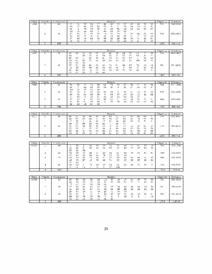
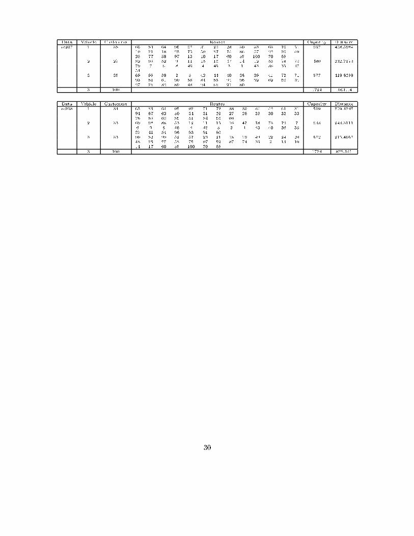
A Appendix

This appendix contains our improvements over the best published solutions at the time of writing(September 1st, 2001).

Data Vehicle Customers Routes Capacity Distance

r108 1 12 28 12 80 76 3 79 78 34 29 24 68 77 169 106.0976

2 11 31 88 10 62 11 64 63 90 32 30 70 154 118.5525

3 13 6 96 59 93 99 5 84 17 45 83 60 18 89 165 84.9083

4 10 52 7 48 82 8 46 47 36 49 19 155 119.9282

5 11 2 57 15 43 42 87 97 95 94 13 58 160 84.6729

6 10 50 33 81 51 9 35 71 65 66 20 153 121.7512

7 12 92 98 91 44 14 38 86 16 61 85 100 37 200 106.0805

8 11 73 72 75 56 23 67 39 55 25 54 26 186 112.2456

9 10 27 69 1 53 40 21 4 74 22 41 116 106.6390

9 100 1458 960.876

Data Vehicle Customers Routes Capacity Distance

r110 1 11 92 98 44 16 86 38 14 37 100 91 93 168 112.0537

2 10 21 72 75 56 23 67 39 25 55 4 172 107.7713

3 11 28 76 12 29 81 79 3 50 77 68 80 188 106.9645

4 9 88 62 19 47 36 49 64 32 70 144 127.5136

5 10 2 41 22 74 73 40 53 26 54 24 108 117.8399

6 9 52 7 82 18 8 46 48 60 89 106 103.7199

7 10 83 45 17 84 5 6 94 96 97 13 138 88.8793

8 11 27 69 30 51 9 71 35 34 78 33 1 130 106.919

9 8 31 11 63 90 10 20 66 65 122 142.3861

10 11 95 59 99 61 85 87 57 15 43 42 58 182 104.7907

10 100 1458 1118.84

Data Vehicle Customers Routes Capacity Distance

rc105 1 4 90 53 66 56 46 73.4507

2 7 63 62 67 84 51 85 91 70 129.2931

3 8 72 71 81 41 54 96 94 93 120 127.5447

4 9 65 82 12 11 87 59 97 75 58 188 142.5070

5 7 33 76 89 48 21 25 24 116 167.0530

6 9 98 14 47 15 16 9 10 13 17 149 121.0211

7 9 42 61 8 6 46 4 3 1 100 132 144.5349

8 9 39 36 44 38 40 37 35 43 70 193 132.9280

9 8 83 19 23 18 22 49 20 77 171 143.0536

10 10 31 29 27 30 28 26 32 34 50 80 183 134.6232

11 8 92 95 64 99 52 86 57 74 114 122.7596

12 5 69 88 78 73 60 95 81.7005

13 7 2 45 5 7 79 55 68 147 108.9662

13 100 1724 1629.44

Data Vehicle Customers Routes Capacity Distance

rc106 1 9 95 62 63 85 76 51 84 56 66 120 109.9733

2 9 72 71 67 30 32 34 50 93 80 127 139.6437

3 11 2 45 5 8 7 6 46 4 3 1 100 193 109.7512

4 8 92 61 81 90 94 96 54 68 125 119.8648

5 8 14 11 87 59 75 97 58 74 161 151.8380

6 9 69 98 88 53 12 10 9 13 17 160 109.3652

7 10 42 44 39 40 36 38 41 43 37 35 200 131.8505

8 9 15 16 47 78 73 79 60 55 70 168 132.3484

9 7 33 31 29 27 28 26 89 125 167.7646

10 10 82 52 99 86 57 22 49 20 24 91 161 120.0993

11 10 65 83 64 19 23 21 18 48 25 77 184 132.2345

11 100 1724 1424.73

Data Vehicle Customers Routes Capacity Distance

r203 1 31 27 94 92 42 57 15 43 14 44 38 86 16 85 484 275.2821

99 96 6 84 8 82 48 47 49 19 63 90 32

10 70 31 7 52

2 40 89 18 60 83 45 46 36 64 11 62 69 88 30 556 368.2665

1 76 3 79 78 9 51 20 66 71 35 68 12

26 13 95 59 93 5 17 61 91 100 98 37 97

58

3 29 50 33 81 65 34 29 24 39 67 23 72 73 21 418 297.8592

40 53 87 2 41 22 75 56 74 4 55 25 54

80 77 28

3 100 1458 941.408

28

Data Vehicle Customers Routes Capacity Distance

r204 1 48 6 94 96 92 97 42 43 15 57 41 22 75 56 712 348.8720

23 67 39 12 76 79 9 51 50 28 53 26 54

55 4 72 74 73 2 13 95 59 93 85 98 37

100 91 16 61 5 60 83 18 89

2 52 27 52 7 88 31 10 30 70 1 69 62 11 19 746 476.6472

46 45 17 86 44 38 14 99 87 84 8 82 48

47 36 49 64 63 90 32 20 66 65 71 35 34

78 81 33 3 77 68 80 29 24 25 21 40 58

2 100 1458 825.519

Data Vehicle Customers Routes Capacity Distance

r207 1 55 95 92 42 91 61 45 46 36 64 11 62 7 88 724 418.6453

69 1 30 51 9 78 79 3 76 28 53 40 2

87 57 41 22 73 21 72 74 75 56 4 25 55

54 80 68 77 12 26 58 13 97 37 100 98 93

59 96 94

2 45 27 50 33 81 65 34 29 24 39 67 23 15 43 734 474.6823

14 44 38 86 16 85 99 6 5 84 8 82 48

47 49 19 10 63 90 32 66 71 35 20 70 31

52 18 83 17 60 89

2 100 1458 893.328

Data Vehicle Customers Routes Capacity Distance

r209 1 31 28 76 12 29 39 67 23 75 72 73 21 40 53 433 304.1939

18 7 62 64 49 36 46 8 45 17 84 96 37

100 91 97 13 58

2 38 52 83 5 59 98 92 95 2 42 14 44 38 86 557 316.3450

16 61 85 93 99 6 94 87 57 15 43 41 22

74 56 4 26 54 55 25 24 80 68 77 1

3 31 27 69 31 88 82 47 19 11 63 90 70 30 71 468 288.6244

9 51 81 33 50 3 79 78 34 35 65 66 20

32 10 48 60 89

3 100 1458 909.163

Data Vehicle Customers Routes Capacity Distance

r211 1 48 28 27 52 69 31 30 63 64 11 19 62 88 7 709 433.4937

82 18 83 84 5 99 85 61 16 44 14 38 86

17 45 8 46 48 47 36 49 90 32 10 70 1

50 77 68 24 55 25 4 56 74

2 52 95 59 92 98 42 15 2 21 73 72 39 67 23 749 459.2191

75 22 41 57 87 94 6 53 40 12 76 29 79

33 81 9 71 65 66 20 51 35 34 78 3 80

54 26 58 13 97 96 37 43 100 91 93 60 89

2 100 1458 892.713

Data Vehicle Customers Routes Capacity Distance

rc205 1 29 2 45 5 42 39 36 72 71 62 94 61 44 40 455 400.1436

38 41 81 90 53 98 55 68 43 35 37 54 96

93 91 80

2 22 92 95 33 28 27 29 31 30 63 76 85 67 84 310 292.3013

51 49 22 20 24 74 13 17 60

3 28 65 83 64 19 23 21 18 57 86 52 99 9 87 566 418.4251

59 75 97 10 66 56 50 34 32 26 89 48 25

77 58

4 21 69 82 11 15 16 47 14 12 88 78 73 79 7 393 186.7777

6 8 46 4 3 1 70 100

4 100 1724 1297.65

Data Vehicle Customers Routes Capacity Distance

rc206 1 32 65 83 52 82 12 14 47 16 15 11 59 75 23 621 335.3131

21 18 19 49 22 57 99 86 87 97 9 10 13

17 60 55 100 70 68

2 35 72 92 95 62 31 29 27 28 30 33 63 85 76 511 476.6132

51 64 84 67 71 94 81 90 66 56 50 34 32

26 89 20 24 48 25 77 58 74

3 33 69 98 2 45 5 44 42 39 38 36 40 41 61 592 334.3909

88 53 78 73 79 7 6 8 46 4 3 1 43

35 37 54 96 93 91 80

3 100 1724 1146.32

29

Data Vehicle Customers Routes Capacity Distance

rc207 1 38 65 83 64 95 67 31 29 28 30 33 63 76 51 667 408.5984

19 21 18 23 75 59 87 74 86 57 22 20 49

25 77 58 97 13 10 17 60 55 100 70 68

2 27 82 99 52 9 11 15 16 47 14 12 53 78 73 480 232.7173

79 7 6 8 46 4 45 3 1 43 36 35 37

54

3 35 69 98 88 2 5 42 44 40 38 39 41 72 71 577 419.8289

93 81 61 90 56 84 85 94 96 92 62 50 34

27 26 32 89 48 24 66 91 80

3 100 1724 1061.14

Data Vehicle Customers Routes Capacity Distance

rc208 1 34 65 83 64 95 92 71 72 38 39 44 42 61 81 519 309.4247

94 67 62 50 34 31 29 27 26 28 30 32 33

76 89 63 85 51 84 56 66

2 33 69 98 88 53 12 11 15 16 47 78 73 79 7 633 243.3111

6 2 8 46 4 45 5 3 1 43 40 36 35

37 41 54 96 93 91 80

3 33 90 82 99 52 57 23 21 18 19 49 22 24 20 572 275.4057

48 25 77 58 75 97 59 87 74 86 9 13 10

14 17 60 55 100 70 68

3 100 1724 828.141

30