Week 3Lesson 2

TW3421x - An Introduction to Credit Risk Management

The VaR and its derivationsSpecial VaRs and the Expected Shortfall

Dr. Pasquale Cirillo

2

An exercise to start with

✤ A 1-year project has a 94% chance of leading to a gain of €5 million, a 3% chance of a gain of €2 million, a 2% chance of leading to a loss of €3 million and a 1% chance of producing a loss of €8 million.What is the VaR for α=0.98? And for α=0.99?

3

The Mean-VaR

✤ Let ! be the mean of the loss distribution. The mean-VaR is defined as

✤ The distinction between VaR and mean-VaR is often negligible in risk management, especially for short time horizons.

✤ For longer time periods (e.g. 1-year), however, the distinction is much more important. In credit risk management, mean-VaR is used to determine economic capital against losses in loans.

V aRmean↵ = V aR↵ � µ

4

Distribution-specific VaRs

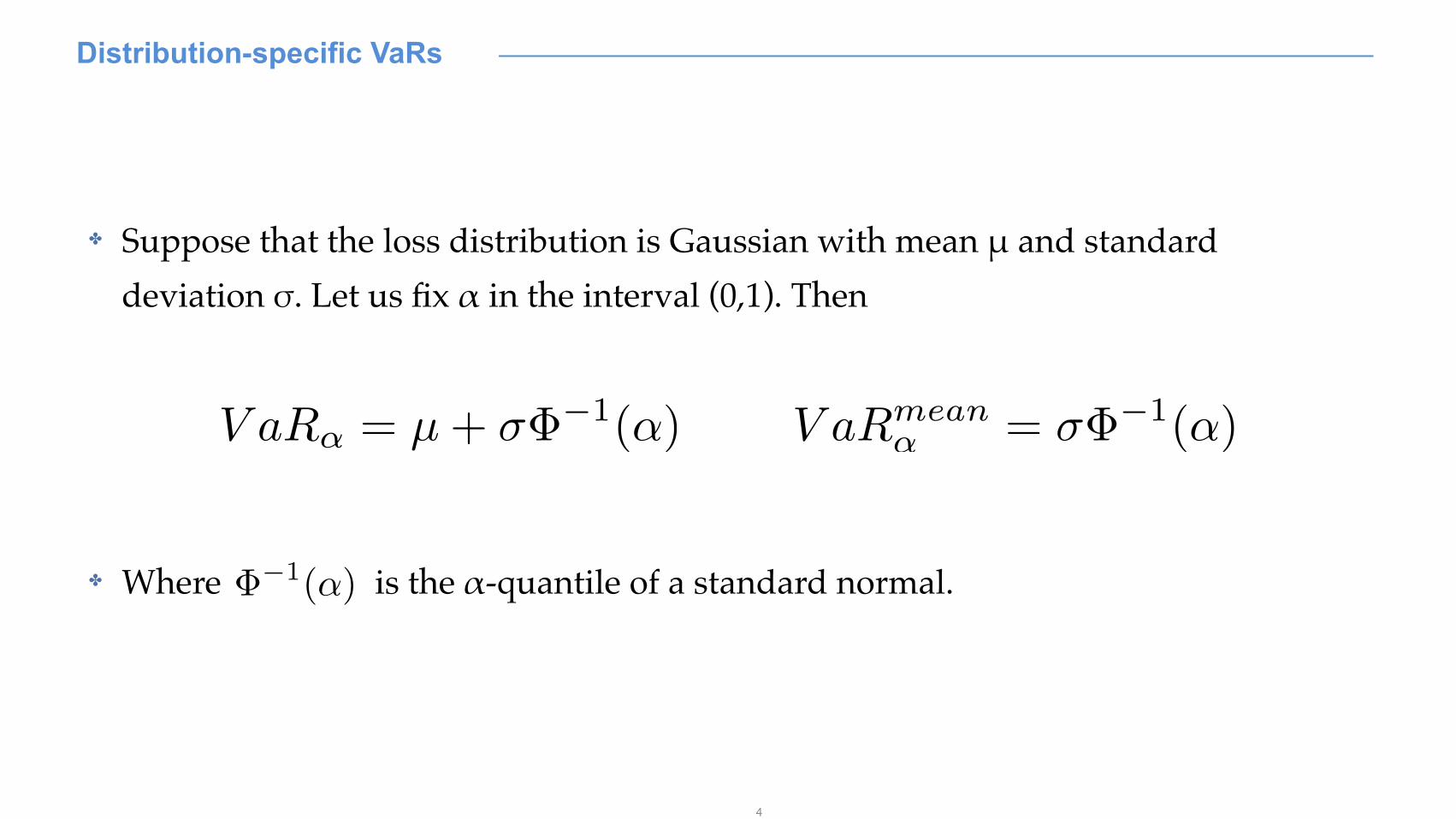
✤ Suppose that the loss distribution is Gaussian with mean μ and standard deviation σ. Let us fix α in the interval (0,1). Then

✤ Where is the α-quantile of a standard normal.

V aR↵ = µ+ ���1(↵) V aRmean↵ = ���1(↵)

��1(↵)

5

Distribution-specific VaRs

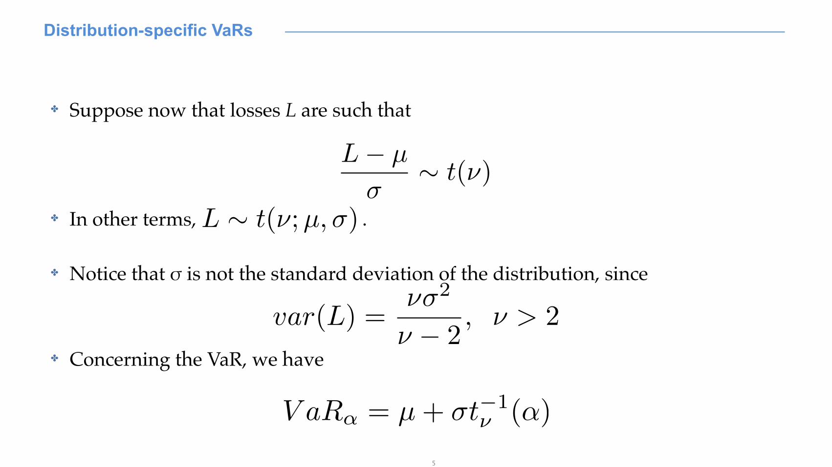
✤ Suppose now that losses L are such that

✤ In other terms, .

✤ Notice that σ is not the standard deviation of the distribution, since

✤ Concerning the VaR, we have

L� µ

�⇠ t(⌫)

L ⇠ t(⌫;µ,�)

var(L) =⌫�2

⌫ � 2, ⌫ > 2

V aR↵ = µ+ �t�1⌫ (↵)

6

Exercise

✤ The historical 1-year loss distribution of a portfolio of loans in € million is well approximated by a N(10,5).What is the 95% VaR? And the 98%?

7

Exercise

✤ The historical 1-year loss distribution of a portfolio of loans in € million is well approximated by a N(10,5).What is the 95% VaR? And the 98%?

✤ Using the standard normal tables or a function such as qnorm in R, we easily find that

✤ Hence:��1(0.95) = 1.6448 ��1(0.98) = 2.0537

V aR0.95(L) = 10 + 5⇥ 1.6448 = 18.2243

V aR0.98(L) = 10 + 5⇥ 2.0537 = 20.2687

8

Exercise

✤ The historical 1-year loss distribution of a portfolio of loans in € million is well approximated by a N(10,5).What is the 95% VaR? And the 98%?

✤ Using the standard normal tables or a function such as qnorm in R, we easily find that

✤ Hence:��1(0.95) = 1.6448 ��1(0.98) = 2.0537

V aR0.95(L) = 10 + 5⇥ 1.6448 = 18.2243

V aR0.98(L) = 10 + 5⇥ 2.0537 = 20.2687

9

The Expected Shortfall

✤ Expected shortfall, aka conditional value at risk, answers to the question

“If things go bad, what is the expected loss?”

✤ It is a measure of risk with many interesting properties.

10

The Expected Shortfall

✤ From a statistical point of view, the expected shortfall is a sort of mean excess function, i.e. the average value of all the values exceeding a special threshold, the VaR!

✤ Why is it important?

ES↵ = E[L|L � V aR↵]

11

The Expected Shortfall

Gain LossV

1-!

Gain LossV

1-!

Same VaR Same VaRDifferent ES Different ES

✤ From a statistical point of view, the expected shortfall is a sort of mean excess function, i.e. the average value of all the values exceeding a special threshold, the VaR!

✤ Why is it important?

ES↵ = E[L|L � V aR↵]

12

Exercise

✤ A portfolio of loans may lead to the losses in the table.

✤ What is the expected shortfall forα=0.95? And α=0.99?

0

0.1

0.2

0.3

0.4

1 2 5 10 12 20 25

Loss ($ 106) Probability1 40%2 35%5 8%10 12%12 2%20 2.5%25 0.5%

13

✤ In the first case we have:

✤ In the second:

Exercise

ES0.95 =12 ⇤ 0.02 + 20 ⇤ 0.025 + 25 ⇤ 0.005

0.05= 17.3

ES0.99 =20 ⇤ 0.005 + 25 ⇤ 0.005

0.01= 22.5

Loss ($ 106) Probability1 40%2 35%5 8%10 12%12 2%20 2.5%25 0.5%

14

✤ In the first case we have:

✤ In the second:

Exercise

ES0.95 =12 ⇤ 0.02 + 20 ⇤ 0.025 + 25 ⇤ 0.005

0.05= 17.3

ES0.99 =20 ⇤ 0.005 + 25 ⇤ 0.005

0.01= 22.5

Loss ($ 106) Probability1 40%2 35%5 8%10 12%12 2%20 2.5%25 0.5%

Trick: move in this direction

5%

15

✤ In the first case we have:

✤ In the second:

Exercise

ES0.95 =12 ⇤ 0.02 + 20 ⇤ 0.025 + 25 ⇤ 0.005

0.05= 17.3

ES0.99 =20 ⇤ 0.005 + 25 ⇤ 0.005

0.01= 22.5

Loss ($ 106) Probability1 40%2 35%5 8%10 12%12 2%20 2.5%25 0.5% 1%

1-α

They sum to 1-α

16

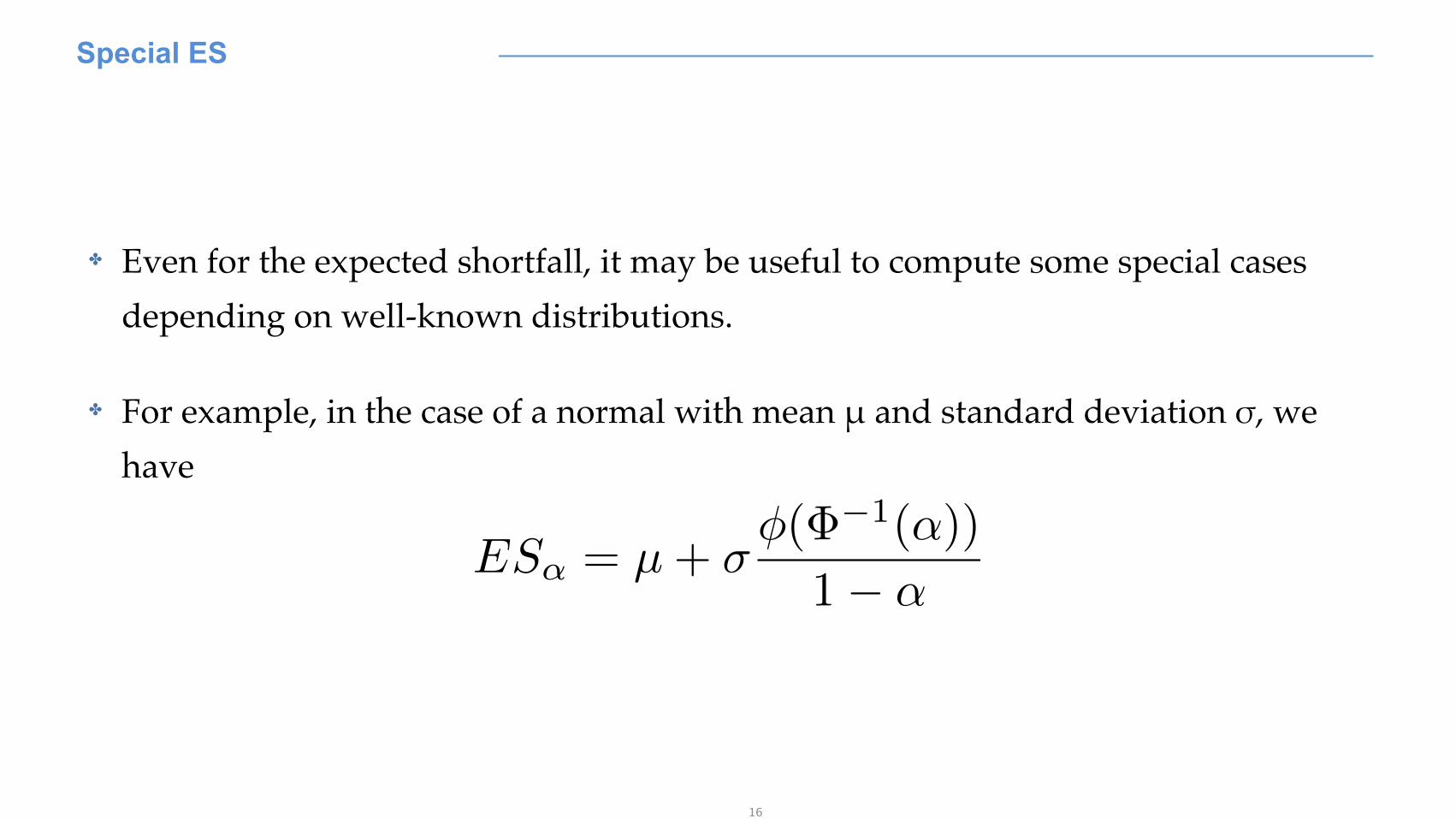
Special ES

✤ Even for the expected shortfall, it may be useful to compute some special cases depending on well-known distributions.

✤ For example, in the case of a normal with mean μ and standard deviation σ, we have

ES↵ = µ+ ��(��1(↵))

1� ↵

Thank You