Twin-float arithmetic

Journal of Symbolic Computation 47 (2012) 536–551

Contents lists available at SciVerse ScienceDirect

Journal of Symbolic Computation

journal homepage: www.elsevier.com/locate/jsc

Twin-float arithmeticJohn Abbott 1Università di Genova, Dipartimento di Matematica, Via Dodecaneso 35, 16146 Genova, Italy

a r t i c l e i n f o

Article history:Received 10 December 2010Accepted 10 May 2011Available online 16 December 2011

Keywords:Heuristically guaranteed finite-precisionarithmetic

a b s t r a c t

We present a heuristically certified form of floating-point arith-metic and its implementation in CoCoALib. This arithmetic is in-tended to act as a fast alternative to exact rational arithmetic,and is developed from the idea of paired floats expounded byTraverso and Zanoni (2002). As prerequisites we need a source of(pseudo-)randomnumbers, and an underlying floating-point arith-metic systemwhere the user can set the precision. Twin-float arith-metic can be used only where the input data are exact, or can beobtained at high enough precision. Our arithmetic includes a to-tal cancellation heuristic for sums and differences, and so can beused in classical algebraic algorithms such as Buchberger’s algo-rithm. We also present a (new) algorithm for recovering an exactrational value from a twin-float, so in some cases an exact answercan be obtained from an approximate computation.

The ideas presented here are implemented as a ring inCoCoALib, calledRingTwinFloat, allowing them to beused easilyin a wide variety of algebraic computations (including Gröbnerbases).

© 2011 Elsevier Ltd. All rights reserved.

1. Introduction and motivation

The principal aim of the arithmetic described in this paper is to obtain quickly a goodapproximation to the exact result of a computation on exact input data (i.e.with rational coefficients).This aim contrasts with that of several recent works which endeavour to tackle problems whoseinput data are approximate (e.g. GCD of approximate polynomials Zeng and Dayton, 2004; Kaltofenet al., 1981). The techniques described in this article are not applicable to problems whose input isapproximate.

The work presented here is a development of ideas proposed by Traverso and Zanoni (2002).Their original goal was to find a fast way of computing a good approximation to a Gröbner basis

E-mail address: [email protected] Tel.: +39 010 353 6890; fax: +39 010 353 6752.

0747-7171/$ – see front matter© 2011 Elsevier Ltd. All rights reserved.doi:10.1016/j.jsc.2011.12.005

http://dx.doi.org/10.1016/j.jsc.2011.12.005

http://www.elsevier.com/locate/jsc

http://www.elsevier.com/locate/jsc

mailto:[email protected]

http://dx.doi.org/10.1016/j.jsc.2011.12.005

J. Abbott / Journal of Symbolic Computation 47 (2012) 536–551 537

(e.g. see Robbiano and Kreuzer, 2000) over the rationals but without the prohibitive cost of therational arithmetic. Direct use of floating point numbers is not possible because recognition of totalcancellation (for sums and differences) is unreliable, yet it is essential to Buchberger’s algorithm.So, they invented the idea of using a pair of floating point values at different precisions: thispermitted heuristically reliable recognition of total cancellation, and also allowed the growth ofrounding error to be monitored. This idea of paired floats2 let them achieve their aim, i.e. tocompute approximate Gröbner bases rapidly: the structure is correct, the coefficients are heuristicallyguaranteed approximations, and the computation is usually fast.

We present twin-float arithmetic, a further development of Traverso and Zanoni’s paired floats,abstracted from the context of Buchberger’s algorithm, and implemented in CoCoALib Abbott andBigatti (2011). During the process of abstraction we resolved some outstanding issues which wereirrelevant in the original context (e.g. see Section 3.6.2. Twin-float arithmetic can be used as a(generally) faster substitute for exact rational arithmetic with a heuristic guarantee of correctness—significant gains in speed are likely if the computation exhibits problems of ‘‘coefficient swell’’, whereinput and output both have small coefficients but intermediate results have much larger coefficients.Many algorithms in computer algebra do indeed exhibit this phenomenon; Buchberger’s algorithm isincluded among these.

A particularly notable addition to twin-float arithmetic (compared to Traverso and Zanoni’soriginal) is the ability to recover a rational number from a twin-float value. This capability allows therecovery of the exact rational answer from a twin-float result under suitable circumstances; e.g. anexact Gröbner basis can be obtained from one computed using twin-floats.

We also give a brief overview of our implementation of twin floats as a ring in CoCoALib: thisopen source C++ library is available from the CoCoA Project’s web-site (Abbott and Bigatti, 2011), andincludes full documentation and several example programs. Twin-float arithmetic will also be readilyaccessible from the forthcoming CoCoA-5 interactive computer algebra system for those who do notwant to grapple with C++.

1.1. An intuitive description of twin-floats

Here we give a brief intuitive outline of twin-floats, the full description with proper definitions isin Section 3. Twin-float arithmetic presupposes the availability of an underlying floating point systemwhere the user may choose the precision. For instance, in CoCoALib the implementation is currentlybased upon the mpf_t type offered by the GMP library (GMP, 2011).

The fundamental idea is that each twin-float value comprises a floating point value together with agood heuristic estimate of its accuracy; the only special case is zero, which is always regarded as beingexact. Before computation begins, the user specifies aminimum acceptable accuracy (see Section 3.2).Every arithmetic operation on twin-float values checks that the heuristically estimated accuracy ofthe result is acceptable (see Section 3.6); if not, the operation fails—in the CoCoALib implementationan exception is thrown. However, an addition or subtraction which results in enough cancellation isregarded as producing exactly zero (see Section 3.6.1).

In general, if a computation on twin-floats does not fail then it produces a result with at least theminimum requested accuracy. However, in very rare cases where theminimum accuracy requested istoo low, the total cancellation heuristic can be fooled. For instance, in our CoCoALib implementationif we specify 12 bits of accuracy then we find that (22619537/15994428)2 − 2 produces exactly zero,a result which is clearly wrong since we know that

√2 is not rational; in fact the true value of the

difference is close to 2−48.

1.2. Comparison with interval arithmetic

A natural question is: how does twin-float arithmetic compare with interval arithmetic? Oneimportant difference is that values in interval arithmetic are always guaranteed correct (i.e. the

2 note that the original name was ‘‘double-float’’, but this might be confused with ‘‘double precision floats’’.

538 J. Abbott / Journal of Symbolic Computation 47 (2012) 536–551

interval surely contains all possible results), whereas twin-float values are only heuristically likelyto be correct to the requested accuracy, or the computation could even fail.

From our point of view, a significant defect of ordinary interval arithmetic is that it does notnaturally recognize total cancellation in sums and differences (with the same strong guarantees ofcorrectness as for the four basic arithmetic operations)—in computational algebra recognition oftotal cancellation is essential (e.g. for computing Gröbner bases). Heuristics for recognizing totalcancellation can be devised, but then the advantages in terms of correctness over twin-floats largelydisappear: in Section 1.2.1 we mention one clever total-cancellation heuristic.

Another problem with interval arithmetic is that the intervals can, and generally do, becomeexcessively large—this is a direct consequence of the strong guarantees of correctness. Overly wideintervals tend to be producedwhen the two operands to an arithmetic operation are not independent.Here is a very simple illustrative example: let X be an interval of width ε then the computation X − Xyields an interval of width 2ε centred on 0. In contrast, thanks to the total-cancellation heuristic inthe rules for twin-float arithmetic (see Section 3.6.1), we will always obtain the exact value zero asthe result of the computation v − v regardless of the twin-float value of v.

A more subtle example where interval arithmetic produces a needlessly wide interval is whencomputing the productY ·(2−Y )with Y = [1−ε, 1+ε].Weobtain the interval [1−2ε+ε2, 1+2ε+ε2

]

which is many times wider than the true interval [1–ε2, 1] when ε is small. In contrast, twin-floatarithmetic recognizes the unusual ‘‘numerical stability’’ of this computation (see Section 3.6.2).

One point in favour of interval arithmetic is that it can be used in cases where the input coefficientsare approximate. Twin-floats cannot be used in such cases. In this article we do not consider furtherthe case of approximate inputs.

1.2.1. Shirayanagi and Sweedler interval arithmeticAn interesting application of interval arithmetic is presented in Shirayanagi and Sweedler (1995).

They call their approach Stabilization of Algorithms. The basic idea is to perform standard intervalarithmetic (with the endpoints being floating point numbers of a specified precision) but with somespecial behaviourwhen evaluating predicates. For instance, the predicatewhich tests whether a valueis zero behaves as follows: if zero does not lie in the interval the result is false; otherwise, when theinterval does contain zero, the interval itself is replaced by the exact value zero (i.e. an interval of zerowidth) and the predicate returns true.

They show that for a wide class of algorithms (which includes polynomial greatest commondivisor and Buchberger’s algorithm) the correct answer will be obtained provided the precisionparameter exceeds a certain bound. Unfortunately it seems to be very difficult to determine, or evenapproximate, this bound. Moreover, the obvious approach of repeating a computation at successivelyhigher precisions until the answer stabilizes is not enough by itself to guarantee that we will getthe right answer—though it is a reasonable heuristic. So, until good bounds can be computed, thetechnique appears to be just an elegant heuristic, and those reassuring theoretical guarantees ofcorrectness remain out of practical reach.

2. Basic definitions and notation

2.1. Denominator

Let q = n/d be non-zero rational number. We define naturally the denominator of q tobe den(q) = |d/ gcd(n, d)|; this is just the positive denominator of the reduced form of q. Forcompleteness we define the denominator of 0 to be 1.

2.2. Relative difference

Let x and x∗ be two (real) values with x being non-zero. We define the relative difference in x∗

from x to be |x − x∗|/|x|. Note that this definition is not symmetric in x and x∗; it may help to think

of x as being an exact value and x∗ an approximation to it, and we want to measure how precise theapproximation is.


2.3. Bits in agreement

As an aid to the reader we define the natural concept of bits in agreement, a little coarser than therelative difference but easy to grasp.

Let x and x∗ be two real values with relative difference ε > 0. Then for any positive integer k suchthat 2−k−1

≥ ε we say that x and x∗ agree to k bits of accuracy. If the relative difference is large,specifically if ε > 1/4, then we do not say that x and x∗ agree at all.

Example. If x = 1 and x∗= 1 − 2−n−1 for some positive integer n then x and x∗ agree to n bits of

accuracy, but not to n+ 1 bits. Similarly, if y = 2 and y∗= 2+ 2−n−1 then y and y∗ agree to n+ 1 bits

of accuracy, but not to n + 2 bits.

2.4. The mapping TF

In Section 3.7 we shall use the notation TF(q) to denote a twin-float value produced by convertingsome rational q according to the method described in Section 3.5. Note that the conversion ofa rational includes the application of a random perturbation, so two separate applications of theconversion to the same rational will very probably produce different twin-float values whichnevertheless will test as being equal to one another (because their primary components will be equal,see Sections 3.4 and 3.5).

3. Definition of twin-float arithmetic

The overall intention of the design was to produce a useful compromise between the speed offinite precision floating-point computations and the unswerving accuracy of rational arithmetic.Achieving both characteristics simultaneously for all computations appears to be impossible (e.g. seethe examples in Section 4). Our compromise is to accept a design which achieves both ‘‘most of thetime’’, but for which there is a (controllably) small chance that we fail to obtain a result, and an evensmaller chance that we obtain a wrong result. The idea is to use heuristics to estimate the accuracyof the result of each individual operation, and if the estimated accuracy is insufficient then failureoccurs—in our CoCoALib implementation an exception is thrown. Similarly we use heuristics to detecttotal cancellation in sums and differences.

3.1. Underlying floating-point arithmetic

Twin-float arithmetic is based upon finite precision floating point representations; it presupposesthe availability of floating point arithmetic where the user can set the precision at run time—but thereis no requirement for user controllable rounding modes. We delegate the responsibility for handlingoverflow and underflow to the underlying floating point implementation. Our CoCoALib softwarecurrently relies on the mpf_t implementation in the GMP library (GMP, 2011); and their approachat the moment is to ignore the phenomena of overflow and underflow and instead offer a numericalrange wide enough for almost all purposes.

3.2. The defining parameters

Twin-float arithmetic is defined in terms of three positive integer parameters A, B and N . Weoutline their meanings here; the precise purposes of these parameters will be made clear inSections 3.5 and 3.6.

• A is mnemonic for accuracy, and is the minimum heuristic bit accuracy for the result of everyindividual arithmetic operation—we shall assume that A ≥ 2.

• B is mnemonic for buffer and specifies the extra accuracy present in a newly created twin-float.The larger B is, the less likely problems of insufficient accuracy will arise.


• N is mnemonic for noise and is used when a new twin-float value is created from a rational. Itdetermines the number of low order noise bits artificially added, viz. between N and 2N bits ofnoise. The value of N should not be too small; e.g. in our CoCoALib implementation we ensure thatN ≥ 16.

3.3. Representation of a twin-float value

A twin-float value is represented as a pair, (V , V ∗), of floating point components of the sameprecision whose values are almost equal. We call V the primary component, and V ∗ the secondarycomponent. The primary component is the approximation produced by the underlying floating-pointsystem to the true value. The secondary component is used to estimate heuristically the accuracy of theprimary component (w.r.t. the unknown true value). So that the algorithms for twin-float arithmetic(especially the one in Section 3.5.1) can work properly the mantissas of V and V ∗ must each have atleast A + B + 2N bits of precision.

Zero has a special representation, (0, 0); it is regarded as being perfectly accurate. All othervalues are represented by two non-zero components. For the representation to be valid, the relativedifference in V ∗ from V must be less than 2−A but no less than 2−A−B−N i.e. we can think of themagreeing to at least A− 1 bits but less than A+ B+N bits. We deliberately exclude pairs with relativedifference less than 2−A−B−N to avoid pitfalls like that exemplified in Section 3.6.2; andwe exploit thislower limit on the relative difference when defining the conversion process in Section 3.7. This lowerlimit should also reduce the influence of rounding error from the underlying floating point arithmetic.

Example. Suppose we are using twin-float arithmetic with A = B = N = 10. Then here is a twin-float value where the relative difference is as large as possible (i.e. almost 2−10 or roughly 3 digits inagreement):

u =

1.2345678901241.235773522829

.

And here is a similar twin float where the relative difference is as small as possible (i.e. just greaterthan 2−30 or roughly 9 digits in agreement):

v =

1.2345678901241.234567891275

.

Wemention briefly an alternative, more compact representation: instead of using the pair (V , V ∗)we could use the pair (V , ε) where ε is the relative difference in V ∗ from V . The main advantage isthat ε could be stored at low precision. At best, this alternative may reduce memory space by a factorof two, and increase speed by a factor of about two. We have not implemented this alternative as theexpected gain is slight, and the extra complication considerable.

3.4. The meaning of twin-floats and the equality test

In this section we present the standard way of interpreting the meaning of a twin-float value,and the closely related concept of ‘‘equality’’ of twin floats. We shall see in Section 3.4.3 that theapproximate nature of twin floats prevents ‘‘equality’’ from being transitive in general. We alsomention in Section 3.4.4 an alternative interpretation which mitigates this lack of transitivity.

To each (non-zero) twin float we shall associate two nested intervals: the inner interval whichprobably contains the true value, and the outer interval which surely contains the true value—here thewords probably and surely are to be understood in a heuristic sense. The utility of these intervals is thatthey form the basis of the equality test. By definition, the outer interval is always at least 2N times aswide as the inner interval, and the inner interval is located centrally in the outer interval. We shalluse these properties in Section 3.7.

We consider the heuristic accuracy of a twin float to be determined by the width of its outerinterval, i.e. by the relative difference in the secondary component from the primary componentwhen


using the Standard Interpretation. In most cases this is a conservative estimate, and the true accuracyis likely to be about N bits greater than the estimate.

3.4.1. Standard interpretationThe special value (0, 0) signifies exactly zero, all other values are non-zero. Let v = (V , V ∗) be a

non-zero twin float. We define its inner and outer intervals as follows:

outer(v) = (V − δ, V + δ) where δ = |V − V ∗|

inner(v) = (V − δ/2N , V + δ/2N).

We highlight the fact that both intervals are centred on V , the primary component. Observe that theratio of the widths of the intervals is essentially constant, having value close to 2N—only the use offinite precision prevents the ratio from being perfectly constant and equal to 2N .

3.4.2. The equality test for twin-floatsWe recall that the equality test is permitted to produce three mutually exclusive outcomes: true,

false, and failure. The outcome failure indicates that it is not possible to determine, with adequatecertainty, whether the two values are equal or unequal. The test is clearly reflexive and symmetric,but not transitive in general, as we shall see in the next subsection. Here is the algorithm:

1. Input: let u and v be two twin-floats.2. If they are both zero then return true.3. If one is zero and the other not then return false.4. If outer(u) ∩ outer(v) = ∅ then return false.5. If inner(u) ∩ inner(v) = ∅ then return true.6. Report failure.

Note: Twin floats can be arithmetically ordered using a slight variation of this algorithm; when theEquality Test returns true the values are equal (of course); when the Equality Test reports failure sodoes the ordering; otherwise the values are unequal and thus trivial to order since the outer intervalsare disjoint.

3.4.3. Failure of transitivity of equalityThe failure of transitivity is hardly surprising since the values concerned are approximate. With

the standard interpretation we can get a ‘‘drastic’’ violation of transitivity of equality: i.e. there existtwin-float values u, v, and w such that u = v and v = w both yield true while u = w yields false.This can happen if the inner interval of v is wide compared to the outer intervals of u and w, morespecifically if |inner(v)| > 1

2 (|outer(u)| + |outer(w)|) and the primary component of u is close to oneend of inner(v) while the primary component of w is close to the other end.

Example. Let the defining parameters be A = B = N = 10, then the following twin-float valuesexhibit the behaviour mentioned above:

u =

1.0249990234391.024999024394

v =

1.0250000000001.024000000001

w =

1.0250009765601.025000975606

v was chosen to have inner interval almost as wide as possible. u and w were chosen to have outerintervals almost as narrow as possible, and such that the primary component of u lies on the lowerend of the inner interval of v while that of w lies on the upper end. It is easy to verify that the outerintervals of u and w are disjoint.


3.4.4. An alternative interpretationHere we mention an alternative interpretation of a twin float which avoid the drastic violation of

transitivity. As in the Standard Interpretation the special value (0, 0) signifies exactly zero, and allother values are non-zero. Let v = (V , V ∗) be a non-zero twin-float value. We define the inner andouter intervals as follows:

outer(v) = (V − ∆, V + ∆) where ∆ = |V |/2A

inner(v) = (V − δ/2N , V + δ/2N) where δ = |V − V ∗|.

Observe that the ratio of the widths of the intervals depends on δ, though it is always at least 2N sinceδ < ∆ for a valid twin float. The inner interval is the same as for the Standard Interpretation. Wecomment that the outer interval does not depend on V ∗; it comprises those numbers whose relativedifference from V is less than 2−A, in other words all valid secondary components.

With this alternative interpretation we cannot get a ‘‘drastic’’ violation of transitivity of equalitybecause it is not possible for one twin float to have its inner interval as wide as the outer interval ofanother twin float having a similar value. Nevertheless a ‘‘mild’’ violation may still occur: i.e. thereexist twin-floats u, v, and w such that u = v and v = w both give truewhile u = w produces failure.

Example. Let the defining parameters be A = B = N = 10, then the following twin-float valuesexhibit the behaviour mentioned above:

u =

1.0249990234391.024999024394

v =

1.0250000000001.024000000001

w =

1.0250009765601.025000975606

.

These are the same values as in the example in Section 3.4.3. The different behaviour comes from thefact that the outer intervals of u and w are much wider than in the Standard Interpretation, and areno longer disjoint.

However, compared to the Standard Interpretation, there is a price to pay. Thewider outer intervalspotentially discard some of the true accuracy of the twin-float values; so as a consequence, someequality tests may ‘‘needlessly’’ produce failure whereas with the Standard Interpretation we wouldhave enough information to be certain that the values were unequal.

Our CoCoALib implementation uses the Standard Interpretation because the benefits of thealternative interpretation are slight while the cost may be significant (because higher precisions maybe needed to avoid failure).

3.5. Conversion of integers and rationals into twin-floats

The first step in computingwith twin-floats is to convert the exact input data (i.e. rational numbers)into twin-float representation. We recall from Section 3.3 that the components of a twin-float musthave at least A + B + 2N bits of precision, otherwise the perturbation process used here (and definedin Section 3.5.1) will not work properly. Here is the algorithm:

1. Input: a rational number q represented as n/d.2. If n = 0 then return TF(q) := (0, 0) the special twin float representing exactly zero.3. Compute the primary component V as n ÷ d in the underlying floating point arithmetic.4. Return the twin float TF(q) := (V , V ∗) where the secondary component V ∗ is determined by the

perturbation process (see Section 3.5.1).

Note: It does not matter whether the input representation n/d is reduced or not. In step (3) some caremay be needed to avoid unnecessary overflow if both n and d are huge.

Note: Applying this conversion process twice to the same rational q will very likely produce twodifferent twin floats because of the randomized perturbation process. However, the equality test(see Section 3.4.2) on these two twin floats will surely produce true because the two primarycomponents are equal.


3.5.1. The perturbation processThe perturbation process lets us generate a valid secondary component from the value in the

primary component. It is used principally when creating a twin-float value from a rational, butmay also be required after an arithmetic operation when the relative difference between the twocomponents of a candidate result is too small (see Section 3.6.2).

We have been given a (finite) floating point value V which will become the primary component ofa twin float, and must determine a suitable secondary component V ∗ to accompany it. This algorithmproduces a V ∗ whose relative difference from V lies between 2−A−B−N and 2−A−B; hence the pair(V , V ∗) is surely a valid twin-float. Here is the algorithm:

1. Input: a non-zero floating point value V .2. Generate a random value ρ uniformly from the set (−1, −2−N

] ∪ [2−N , 1).3. Return V ∗

= V · (1 + 2−A−Bρ).

Note: Since we are using finite precision arithmetic with A + B + 2N bits, in Step (2) we need togenerate just the first 2N bits of ρ. Indeed, if a source of random integers is available, one way toimplement Step (2) is as follows: generate a random integer R in the range {−22N

+ 1, . . . , 22N− 1};

if we find that |R| < 2N , go back and generate another one; otherwise set ρ = R/22N .

3.5.2. Differences from Traverso and Zanoni’s methodThe main feature in common between our method and that of Traverso and Zanoni (abbr. TZ) is

that each value is represented as a pair of floating point numbers whose relative difference is used toestimate heuristically the precision. The description of the TZ method in Traverso and Zanoni (2002)is rather brief and vague (e.g.we believe their total cancellation heuristics are more or less equivalentto ours, which is clearly described in Section 3.6.1). Nevertheless we can identify two significantdifferences between the methods:

• Ourmethod involves randomization, and as a consequence there are some computationswhich cangive different results if repeated (e.g. see Section 5.1). In contrast, the TZ method is deterministic(assuming that the underlying floating point arithmetic is).

• Our definition of valid twin float places both upper and lower limits on the relative difference,and ensuring the lower limit in the result of an arithmetic operation may require special action(see Section 3.6.2). In contrast, in the TZ method there is no lower limit on the relative difference;indeed it may even become zero—implying infinite accuracy, a rather improbable occurrence.

3.6. Rules of arithmetic

In outline, to combine two twin floats arithmetically, we produce a candidate result by applyingthe operation separately to the primary components and the secondary components, and then verifythat the candidate is valid; in the case of addition or subtraction we conduct a special check for totalcancellation.

1. Input: two twin floats u = (U,U∗) and v = (V , V ∗), and an arithmetic operation •

2. Handle the cases where u = 0 and/or v = 0 specially.3. If • is addition or subtraction, apply the Total-Cancellation Heuristic: perform the equality test

(see Section 3.4.2) on u and ∓v; if it reports failure then report failure; if it returns true then return(0, 0).

4. Compute the components of the candidateW = U • V andW ∗= U∗

• V ∗.5. If the relative difference inW ∗ fromW is at least 2−A then report failure.6. Apply the check in Section 3.6.2 to ensure that the relative difference is not too small.7. Return the twin float w = (W ,W ∗) as the result.


3.6.1. Total-cancellation heuristic for addition and subtractionIn exact arithmetic we have a logical equivalence: given two values X and Y , then X = Y if and

only if X − Y = 0. Unfortunately, with twin-float arithmetic we do not have such a clear and simpleequivalence because any operation on twin floats may report failure instead of giving a result. Thenext example shows that there are even twin-float values where one side of the equivalence must failbut the other side does not.

Example. Here we see two twin-float values which are obviously unequal but for which wecannot calculate their difference with (at least) the specified minimum accuracy. We suppose thatthe requested accuracy is A = 10 bits (i.e. about 3 decimal digits); the values of the parametersB and N are unimportant. Consider the two twin float values v = (0.999999, 0.999876) andw = (0.990000, 0.990123). Now the test u = v surely produces false, yet we cannot compute thedifference v − w with 10 bits of accuracy, so trying to do so must produce failure.

So in twin-float arithmetic the relationship between equality and subtraction is a bitmore complex.We want our definitions to retain as much coherence as possible between equality and subtraction.Here is the best we can achieve:

• The computation v − w produces 0 if and only if the test v = w yields true.• If v − w produces a non-zero value then v = w yields false.

For convenience we mention two direct consequences of these rules which illustrate explicitly thepossible relationships when failure occurs:

• If the test v = w produces failure then the computation v − w will too.• If the computation v − w produces failure then the test v = w may produce either failure or false.

An immediate implication of these rules is that the test for total cancellation in addi-tion/subtraction must be identical to the criterion used when the equality test yields true. So in Step(3) of the general arithmetic algorithm of Section 3.6 when performing addition or subtraction oftwin-floats, we first perform an equality test on the arguments (negating one of them for addition).If the equality test says they are equal then the operation produces zero; if the equality tests reportsfailure then so does the addition/subtraction operation. Otherwise we compute the candidate resultand perform the usual validity check.

3.6.2. A lower limit for the relative differenceThe apparently trivial task of dividing a (non-zero) twin-float value by itself leads to a surprisingly

delicate situation. According to the Rules of Arithmetic, we begin by computing a candidate result,w = (1, 1) in this case. Note that both components of w are exactly 1. Now, the heuristic accuracy isdetermined by the relative difference between the components, which is zero in this case, implyinginfinite accuracy. So far there are no problems. The example below shows why the value w is‘‘dangerous’’.

Example. We now show how the twin-float w = (1, 1) can lead to problems. Suppose that w isallowed as a valid twin-float value. Then we can compute x = w/(w +w +w) whose representationas a twin-float is x = (X, X) where X is the underlying floating-point representation of 1/3. But withbinary arithmetic the value X is only approximate, not exactly equal to 1/3. The difficulty is nowevident: since both components of x are identical, we deduce an infinite heuristic accuracy whichis no longer a realistic estimate. This value x is ‘‘dangerous’’ because it has essentially disabled theheuristic accuracy check, and so subsequent computation with it could well lead to results with quitemisleading accuracy estimates.

Admittedly the operation of dividing a value by itself may seem rather pointless, but in fact it caneasily arise in computation (e.g. when making a polynomial monic). So it is not feasible to avoid theproblem by simply producing failurewhenever dividing a value by itself; if we did so, we would neversucceed in making a polynomial monic at any precision! Instead we choose to avoid the problemby outlawing values like w which ‘‘have too much heuristic accuracy’’. We employ the following


simple technique. After each arithmetic operation we check the relative difference between the twocomponents of the candidate result. If the relative difference is less than 2−A−B−N then we generatea new secondary component by applying the perturbation procedure (see Section 3.5.1), therebyproducing a valid twin-float value.

3.7. Conversion of twin-floats into rational numbers

In this section we look at the problem of converting a twin-float value into an exact rational value.The principal motivation is to allow, when possible, an exact rational result to be obtained from acomputation performed using twin-floats. We shall concentrate on the task of converting a singletwin-float value into a rational (without any further knowledge about the rational, e.g. knowing aprescribed denominator).

Let v = (V , V ∗) be the twin float to be converted into a rational. We may assume that v is non-zero, otherwise conversion is trivial. By the definition of twin float arithmetic, we normally expect theprimary component, V , to be the better approximation to the true value. So a reasonable (and fast)answer is simply to return V as the rational—recall that every float is a rational.We reject this solutionbecause the denominator is restricted to being a power of 2 (or perhaps of 10); thus, for instance, wecould never obtain the simple rational 1/3 however high an accuracy we might use.

This example leads us naturally to the idea that wewant to obtain the ‘‘simplest rational’’ possible.So for instance, we would intuitively prefer the answer 1/3 to the answer 33333/100000 if bothare valid candidates; and between these two we would say that 1/3 is ‘‘clearly the right rational’’.However, with certain other values (e.g. those very near

√2, which we know is not rational) there

may be no clear choice, and so in such cases wemay prefer to signal failure rather than give an answerwhich is not ‘‘clearly the right one’’.

Before proceedingwemake rigorous the intuitive notion of simplicity for rationals. Given two non-zero rationals q1 and q2 we say that q1 is simpler than q2 if den(q1) < den(q2); this is only a partialorder, but sufficient for our needs.

3.7.1. Desirable characteristicsBearing in mind the brief discussion above, we summarize here the main characteristics which we

would like the conversion operation to have—in essence, the conversion must produce the simplestrational it can, and must succeed whenever reasonably possible.

(a) Like any other operation on twin-floats the attempted conversion may result in failure. But theconversion must succeed if there is a sufficiently simple rational q for which the Equality Teston v and TF(q) yields true.

(b) If the conversion of a twin-float v does succeed (and produces q ∈ Q) then the Equality Test onTF(q) and v yields true.

(c) If two twin-floats v and w can both be converted into rationals (qv and qw resp.) and the EqualityTest on v and w always (see Section 5.1) yields true then qv = qw .

(d) Let v be a twin-float which can be converted into a rational q; and let Q be another rational suchthat the Equality Test on TF(Q ) and v yields true then q is simpler than or equal to Q .

(e) If the conversion of a twin-float v does succeed (and produces q ∈ Q) and let q′∈ Q be a simpler

rational than q then the Equality Test on TF(q′) and v yields false.

3.7.2. Clearly the right rationalWe now turn to the definition of the heuristic ‘‘clearly the right one’’. Let v be a non-zero twin-

float. We say that the (reduced) rational q is ‘‘clearly the right one’’ if TF(q) = v yields true and wehave den(q′) > 2N−2 den(q) for any other rational q′ where the Equality Test on TF(q′) and v yieldstrue. In other words, our chosen rational q is much simpler than any other candidate satisfying (b).


3.7.3. Finding the simplest rational in an intervalOur conversion algorithm (in Section 3.7.4) will need to determine the simplest rational in a non-

empty closed interval [a, b]—a task which is readily achieved by converting a and b into continuedfractions (e.g. seeHardy andWright, 1979 for definitions andmany useful properties). For this task, wesummarize here a simple method which was certainly known in 1981 (see Gosper, 1981); however,given its simplicity, it seems likely that it is considerably older. The correctness of this method isimmediate from basic properties of continued fractions.

If 0 ∈ [a, b] then 0 is surely the simplest rational. If b < 0, it suffices to find the simplest rationalin the interval [−b, −a] and then negate it. We can now restrict to the case 0 < a < b.

Let [a0, a1, . . .] be the sequence of continued fraction partial quotients for a; similarly let[b0, b1, . . .] be that for b. If one sequence is a prefix of the other then the simplest rational is theend-point with the shorter sequence. Otherwise set k to be the first index where ak = bk. If ak < bkand the sequence for a ends at ak then a is the simplest rational; analogously, if bk < ak and thesequence for b ends at bk then b is the simplest rational. In every other case the simplest rational isthe one whose sequence of partial quotients is [a0, a1, . . . , ak−1, α] where α = 1 + min{ak, bk}.

Example. We show the determination of the simplest rational between 0.68 and 0.74. The respectivecontinued fraction partial quotient sequences are [0, 1, 2, 8] and [0, 1, 2, 1, 5, 2]. In this case neithersequence is a prefix of the other. The sequences first disagree in the fourth position. While onesequence does end at the fourth partial quotient, the corresponding end-point is not the simplestrational because the other sequence has a smaller partial quotient in that position. Thus we are in thegeneral case, and the simplest rational has partial quotient sequence [0, 1, 2, 1 + 1], in other wordsit is 5/7.

3.7.4. Algorithm for converting a twin-float to a rational1. Input: Let v be a twin float.2. If v is zero, return 0.3. If outer(v) contains two or more integers, report failure—there is no obviously simplest rational.4. Let q be the simplest rational in the interval outer(v)—e.g. using the method in Section 3.7.3.5. If q ∈ inner(v) then return q, otherwise report failure.

We shall now show that when this algorithm produces a rational number it is ‘‘clearly the rightone’’. Let q be the rational number produced by the algorithm. We deal first with the special caseswhere den(q) = 1 or den(q) = 2.

In the case den(q) = 1 we know that |outer(v)| < 2 because outer(v) contains just one integer.Hence |inner(v)| < 2−N+1, and so any other rational lying inside inner(v) must have denominatorgreater than 2N−1.

In the case den(q) = 2 we know that |outer(v)| < 1 because outer(v) contains no integer. Hence|inner(v)| < 2−N , and so any other rational lying inside inner(v)must have denominator greater than2N−1.

For the general case of den(q) > 2 we shall use the following two lemmas.

Lemma A. Let n/d, n′/d′∈ Q be distinct rationals. Then |n/d − n′/d′

| ≥ 1/dd′.

Lemma B. Let n/d ∈ Q be in reduced form with d ≥ 3. Then there exists a simpler rational n′/d′∈ Q

such that |n/d − n′/d′| ≤ 2/d(d + 1).

Proof. Thismay easily be deduced fromwell-knownproperties of neighbouring elements in the Fareysequence for d. See Theorems 28 and 30 in Hardy and Wright (1979). �

Let d = den(q), so we can write q = n/d. We know that q ∈ inner(v) and that inner(v) iscentrally located in outer(v). Let W be half the width of outer(v); and thus inner(v) has width atmost 21−NW . Using Lemma B and the fact that q is the simplest rational in outer(v) we see thatW < 2/d(d + 1). Now let q′

= n′/d′∈ inner(v) be another rational. Applying Lemma A, we

see that 1/dd′≤ |n/d − n′/d′

| < 21−NW , where the right hand side is the upper bound for the


width of inner(v). Hence d′ > 2N−1/Wd > 2N−2(d + 1). In other words we have proved thatden(q′) > 2N−2 den(q), and so q satisfies the condition for being ‘‘clearly the right one’’.

The rational conversion effected by our algorithm enjoys fully characteristics (a) and (b), and formost practical purposes enjoys (c), (d) and (e) as well. Strictly, to obtain fully characteristic (d) wewould have to modify the algorithm by replacing the final check q ∈ inner(v) with a membershipcheck of a slightly wider interval containing all rationals q′ for which the Equality Test on TF(q′) and vyields true (with probability 1). To obtain characteristic (e) we would need to modify the algorithmto search for the simplest rational in an interval slightly wider than outer(v) which contains allrationals q′ for which the Equality Test on TF(q′) and v does not produce false (with probability 1).Characteristic (c) poses a different sort of problem, related to the imperfect transitivity of the EqualityTest.

3.7.5. Converting a twin-float to the wrong rationalThe conversion of a twin-float value into a rational number involves the heuristic criterion that we

have nicknamed ‘‘clearly the right one’’. This heuristic can occasionally be fooled into giving a falsepositive. In realitywrong results seem very rare, but it is difficult to quantify the likelihood: it dependson the presence of large continued fraction partial quotients in the rationalwe are computing.Wenowconstruct a case designed to trick the heuristic.

Pick any twin-float arithmetic (i.e. fix the parameters A, B and N), and call it R. Now let W be apositive integer for which u and u + TF(2−W ) must have the same internal representation where umay be any image of 1 in R; that isW is so large that 2−W is negligible compared to 1 in the underlyingfloating point representation.

So if we use R to compute TF(1)+TF(2−W ), and then convert the result into a rational number, theconversion will succeed and produce the incorrect rational number 1. Conversely, if we use a higherprecision twin-float arithmetic (e.g.with parameterA > W ) then conversionwill successfully producethe correct rational, namely (2W

+ 1)/2W .The example above is just a specific instance of a general case: the heuristic criterion can be fooled

if the rational to be recovered has a sufficiently large continued fraction partial quotient. Let q bea rational number which has an especially large partial quotient, say Q . The presence of the largepartial quotient means that q can be written as the sum of a simple fraction and a complex one of verysmall magnitude, that is q = q1 + q2 where the second summand satisfies |q2| < 1/Q den(q1)—seetheorem 163 in Hardy and Wright (1979). In other words, the simple fraction q1 is an exceptionallygood approximation to q. If the relative difference between q and q1 is small enough (e.g. about2−A−B−N ) then the twin-float arithmetic will regard q and q1 as being equal, and the rational recoverywill erroneously produce q1 as its result.

4. Some tricky cases

While twin-float arithmetic does model rational arithmetic well enough for many purposes, it isnonetheless possible to construct computations which fool the heuristics, and thus lead to wronganswers. Here are some contrived examples.

4.1. Lack of associativity

It is well-known that floating-point arithmetic does not enjoy all the properties of exact arithmetic,and since twin-floats are built on top of (normal) floats they inherit some of these defects. For instance,addition is not associative: e.g. (1 + (−1)) + 2−1000

= 1 + (−1 + 2−1000) if we compute with fewerthan 1000 bits of precision. Similarly, multiplication is not associative: e.g. (21000

× 21000) × 2−1000=

21000× (21000

× 2−1000) in standard ‘‘double precision’’ arithmetic since overflow occurs in one casebut not the other. Occasionally even the wide range of mpf_t in the GMP library is insufficient: e.g. ona 32-bit computer, we encountered problems computing the factorial of 109 using the twin-floatimplementation in CoCoALib.


4.2. Summing values of widely differing magnitude

With limited precision arithmetic a sum of the form 1+ ε poses a problemwhen ε is so small thatthe best approximation to the true answer is 1. This implies that for almost any value x there existsy > 0 such that x + y = x, an absurdity in exact arithmetic.

In twin-float arithmetic we have the option of producing failure instead of a numerical result; sowe could declare that summing two values which differ too widely in magnitude will fail. However,in many cases it is fine to produce the value 1 for the sum 1 + ε when ε is very small. Difficultiesarise only if we subsequently want to compare that result with exactly 1; a very rare occurrencein our experience. Consequently, our implementation does not report failure when one summand isnegligible.

Here we see two tricky examples where reporting failure for negligible summands would notresolve the problem anyway.

Example. It is easy to produce values of the form 1 + ε without overtly computing a sum with anegligible value. Let k ∈ N; we show how to obtain 1 − 2−k by summing only values of similarmagnitude. Start with s0 = 2−k then successively compute sj = sj−1 + 2j−k for j = 1, . . . , k − 1.The final value is sk−1 = 1 − 2−k, but all additions involved numbers differing in magnitude by atmost a factor of 2.

Example. Here is another way of producing values of the form 1 + ε; this time we use justmultiplication and subtraction between numbers differing in magnitude by about a factor of 2.

Define the sequence an by a0 =12 and an = an−1(2 − an−1) for n ≥ 1. It is easy to show that

an = 1−2−2n in exact arithmetic. If we were to compute the sequence using finite precision floats, atsome point we will obtain exactly 1. Twin-floats will behave the same way. Moreover, it is not clearhow some sophisticated finite precision arithmetic could obtain a sensible non-zero value for 1−a100,say.

5. Characteristic behaviour

In this section we look at some aspects of the behaviour of twin floats. In particular we areinterested in behaviour peculiar to thisway of performing arithmetic. One remarkable outcome is thatsuccessful completion of a computation at one precision does not guarantee successful completion ofthe same computation at a higher precision—nevertheless the probability of successful completiondoes increase with increasing precision.

5.1. Testing equality of nearly equal values

Consider the following three subprograms (written in pseudo-code) each of which has a singlerational number parameter.

SubprogramA(eps):TwinFloat X = 1;return X == X+eps;

SubprogramB(eps):TwinFloat X = 1;TwinFloat Y = 1 + eps;return X == Y;

SubprogramC(eps):TwinFloat X = 1;TwinFloat Y = 1 + eps;return IsZero(X-Y);


Superficially the three subprograms appear all to do the same thing, namely testwhether 1+ε = 1where ε is passed as a parameter. We shall study briefly the behaviour of these subprograms as thevalue of the parameter is varied, and for simplicity we shall suppose that the parameter is an exactrational. It is clear that for sufficiently large values all three subprograms will return false; and forvalues sufficiently close to zero they will all return true (since the internal representation uses finiteprecision).

Let us see what happens when we pass the value ε = 2−B as parameter. SubprogramA andSubprogramB will return false. In contrast, SubprogramC may return false or it may fail. Failurewill occur if there is too great a relative difference between the two components of the candidatevalue for the difference X−Y. The relative difference is 2−A(ρX − ρY ) where ρX and ρY are therandomperturbations usedwhen creatingX and Y respectively. SinceρX andρY are chosen essentiallyuniformly in the open intervals (−1, 1) and (−1−ε, 1+ε) respectively, there is a probability of about1/4 that the computation fails because the relative difference exceeds 2−A. In fact SubprogramCmayfail also for larger values of the parameter: indeed, a similar argument shows that there is a (low)probability of about 2−2B of failure when called with parameter ε = 21−B.

We now consider what happens when the parameter value is 2−A−B. We find that SubprogramAand SubprogramB may return false or they may fail. We look in detail at what happens inSubprogramA; the inner workings of SubprogramB are similar but a bit messier. The equality testreturns false if and only if the outer intervals are disjoint. We have outer(X) = (1 − 2−A−BρX , 1 +

2−A−BρX ) while outer(X + ε) ≈ (1 + 2−A−B(1 − ρX ), 1 + 2−A−B(1 + ρX )). These two intervalswill intersect if ρX > 1/2, which happens with probability 1/2. The explanation of the behaviourof SubprogramC is a little more complex because the subtraction can fail for two different reasons:the relative error in the candidate result could be too great, or the total-cancellation heuristic (seeSection 3.6.1)may report failure. LetρX andρY be the randomperturbations usedwhen creating X andY ; without loss of generality wemay assume that these perturbations are positive. The outer intervalsare outer(X) = (1−2−A−BρX , 1+2−A−BρX ) and outer(Y ) = (1+2−A−B(1−ρY ), 1+2−A−B(1+ρY )).Thesewill have non empty intersection if and only ifρX+ρY > 1, a condition satisfiedwith probability1/2. If the intersection is non empty then the total-cancellationheuristicwill trigger a failure (meaningthat the result might be zero but one cannot be sure using twin-float arithmetic with the specifiedA and B parameters). If the intersection is empty, we know the result is non-zero, but must thencheck that the relative difference is not too large. In this case the relative difference is |ρY − ρX |.The computation will fail unless the relative difference is less than 2−A, and this will happen withprobability about 2−A−1.

All three subprograms will start producing true when the supplied parameter ε value falls below21−A−B−N , i.e.when the inner intervals of the twin float images of 1 and 1 + ε might have non emptyintersection. When the parameter is smaller than 21−A−B−2N all three subprograms will produce truewith high probability; failure may still be possible, but the precise behaviour will depend on theactual precision used in the underlying floating point arithmetic, and perhaps also the way valuesare rounded.

6. Example: Muller’s recurrence

Here we look at Muller’s (infamous) recurrence3 (see p. 48 of Muller, 1989) which was created toillustrate one of the perils of computing with limited precision. The sequence is defined as follows:

a0 = 2a1 = −4an = 111 − 1130/an−1 + 3000/an−1an−2 for n > 1.

If we compute this sequence using double-precision floating point arithmetic, it converges swiftlyto 100. If we try again at higher precision (e.g. 100 decimal digits), it converges swiftly again to 100.

3 I have changed the initial values to integers so that they are exactly representable in binary.


Indeed, no matter what precision we try, we always get the same result. Intuitively this leads us tobelieve that we have a guarantee of correctness of the result.

It might come as a surprise then to discover that it is not hard to prove that the sequence anconverges to 6. But with any finite precision arithmetic explosive growth of a spurious solutionderiving from rounding error forces numerical convergence to 100.

One of the CoCoALib example programs, ex-RingTwinFloat2.C, shows the behaviour of twin-float arithmetic in this computation. The program tries increasing levels of precision, and alwaysreports failure (i.e. it throws anInsufficientPrecision exception). As supplied, the program setsthe two defining parameters A and B to the same value, but modifying it to set the value of B explicitlyto about 22 · A allows the convergence to 6 to be recognized thanks to the large buffer space. Thecrucial point is that no matter how wemodify the choices of the defining parameters in the program,it will never wrongly report convergence to 100.

Below we present one way of implementing Muller’s sequence using CoCoALib. This functionexpects a CoCoALib ring (R should be an instance of twin-float arithmetic). The predicateIsPracticallyEqual produces true if its two arguments test as equal, otherwise it producesfalse—it never reports insufficient precision. The function as a whole will either fail due toinsufficient precision (triggered while trying to evaluate the expression for Vcurr), or will returnan approximation to the value the sequence appears to be converging towards.

RingElem MullerSeq(ring R){

RingElem Vprev1(R, -4);RingElem Vprev2(R, 2);

while (!IsPracticallyEqual(Vprev1, Vprev2)){

RingElem Vcurr = 111 - 1130/Vprev1 + 3000/(Vprev1*Vprev2);Vprev2 = Vprev1;Vprev1 = Vcurr;

}return Vprev1;

}

int main(){

for (int BufferBits = 650; BufferBits <= 750; ++BufferBits){

ring R = NewRingTwinFloat(32,BufferBits,32); // params are A,B,Ntry { cout << "BufferBits=" << BufferBits << " & value=" << MullerSeq(R) << endl; }catch (const RingTwinFloat::InsufficientPrecision&){ cout << "Failed with BufferBits=" << BufferBits << endl; }

}}

When we run the program above we find that when BufferBits is less than about 670 the functionMullerSeq always fails due to insufficient precision; in contrast, once the number of buffer bits passes about720 the function MullerSeq always produces a value very close to 6: specifically, an equality test between thevalue produced and 6 produces either true or failure (but not false).

7. A few benchmarks

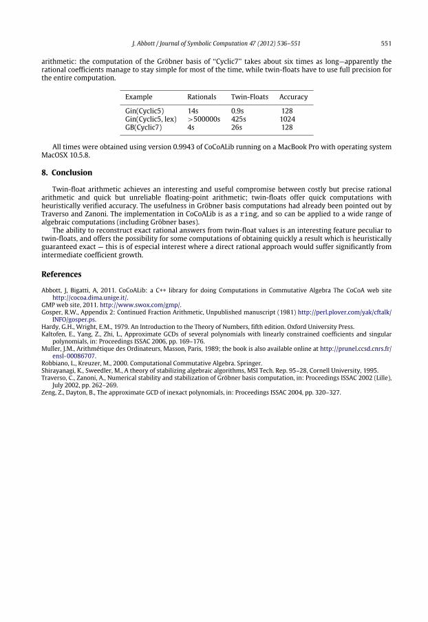
Here are a few benchmarks comparing computation times over the rationals with times for the samecomputation using twin-floats. The column headed ‘‘Accuracy’’ indicates the common value used for the twin-float parameters A and B (N was kept fixed at 32). It is not usually obvious what accuracy to request: toolow and failure will result, too high and time is wasted handling high precision values. We adopted a simpleapproach: initially requesting 64 bits, and if failure occurred at some point, we restarted the computation(possibly repeatedly) each time doubling the requested accuracy, until an answer was obtained.

The ‘‘gin’’ (generic initial ideal) examples show that twin-float coefficients can lead to enormously fastercomputing times than with rational coefficients: effectively we compute a Gröbner basis after applying a‘‘generic’’ (i.e. random) change of coordinates. In contrast we see that sometimes twin floats do not beat rational


arithmetic: the computation of the Gröbner basis of ‘‘Cyclic7’’ takes about six times as long—apparently therational coefficients manage to stay simple for most of the time, while twin-floats have to use full precision forthe entire computation.

Example Rationals Twin-Floats Accuracy

Gin(Cyclic5) 14s 0.9s 128Gin(Cyclic5, lex) >500000s 425s 1024GB(Cyclic7) 4s 26s 128

All times were obtained using version 0.9943 of CoCoALib running on a MacBook Pro with operating systemMacOSX 10.5.8.

8. Conclusion

Twin-float arithmetic achieves an interesting and useful compromise between costly but precise rationalarithmetic and quick but unreliable floating-point arithmetic; twin-floats offer quick computations withheuristically verified accuracy. The usefulness in Gröbner basis computations had already been pointed out byTraverso and Zanoni. The implementation in CoCoALib is as a ring, and so can be applied to a wide range ofalgebraic computations (including Gröbner bases).

The ability to reconstruct exact rational answers from twin-float values is an interesting feature peculiar totwin-floats, and offers the possibility for some computations of obtaining quickly a result which is heuristicallyguaranteed exact — this is of especial interest where a direct rational approach would suffer significantly fromintermediate coefficient growth.

References

Abbott, J, Bigatti, A, 2011. CoCoALib: a C++ library for doing Computations in Commutative Algebra The CoCoA web sitehttp://cocoa.dima.unige.it/.

GMP web site, 2011. http://www.swox.com/gmp/.Gosper, R.W., Appendix 2: Continued Fraction Arithmetic, Unpublished manuscript (1981) http://perl.plover.com/yak/cftalk/

INFO/gosper.ps.Hardy, G.H., Wright, E.M., 1979. An Introduction to the Theory of Numbers, fifth edition. Oxford University Press.Kaltofen, E., Yang, Z., Zhi, L., Approximate GCDs of several polynomials with linearly constrained coefficients and singular

polynomials, in: Proceedings ISSAC 2006, pp. 169–176.Muller, J.M., Arithmétique des Ordinateurs, Masson, Paris, 1989; the book is also available online at http://prunel.ccsd.cnrs.fr/

ensl-00086707.Robbiano, L., Kreuzer, M., 2000. Computational Commutative Algebra. Springer.Shirayanagi, K., Sweedler, M., A theory of stabilizing algebraic algorithms, MSI Tech. Rep. 95–28, Cornell University, 1995.Traverso, C., Zanoni, A., Numerical stability and stabilization of Gröbner basis computation, in: Proceedings ISSAC 2002 (Lille),

July 2002, pp. 262–269.Zeng, Z., Dayton, B., The approximate GCD of inexact polynomials, in: Proceedings ISSAC 2004, pp. 320–327.

http://cocoa.dima.unige.it/

http://www.swox.com/gmp/

http://perl.plover.com/yak/cftalk/INFO/gosper.ps









http://prunel.ccsd.cnrs.fr/ensl-00086707






Documents

Twin-float arithmetic