Embed Size (px)
Citation preview

Twin Subsequence Search in Time SeriesGeorgios Chatzigeorgakidis
IMSI, Athena R.C.
Dimitrios Skoutas
IMSI, Athena R.C.
Kostas Patroumpas
IMSI, Athena R.C.
Themis Palpanas
LIPADE, Université de Paris &
French University Institute (IUF)
Spiros Athanasiou
IMSI, Athena R.C.
Spiros Skiadopoulos
DIT, University of Peloponnese
ABSTRACTWe address the problem of subsequence search in time series us-
ing Chebyshev distance, to which we refer as twin subsequence
search. We first show how existing time series indices can be ex-
tended to perform twin subsequence search. Then, we introduce
TS-Index, a novel index tailored to this problem. Our experi-
mental evaluation compares these approaches against real time
series datasets, and demonstrates that TS-Index can retrieve twin
subsequences much faster under various query conditions.
1 INTRODUCTIONGiven a time series 𝑇 and a query sequence 𝑄 (|𝑄 | ≪ |𝑇 |), sub-sequence search finds subsequences in 𝑇 that are similar to 𝑄 .
Although most works rely on Euclidean distance or Dynamic
Time Warping (DTW) (e.g., [17, 19]), different L𝑝 norms or other
similarity measures are also useful for capturing different pat-
terns of similarity or achieving higher classification accuracy
in certain datasets [6, 22]. In this work, we use the Chebyshevdistance (i.e., L∞ norm) between two subsequences, which is
the maximum difference of their values across their entire dura-
tion. We call two subsequences twins with respect to a distance
threshold 𝜖 , if their Chebyshev distance is not greater than 𝜖 . This
kind of similarity search can be useful is various applications:
finding doublet earthquakes in seismology, identifying similar
traffic patterns in road networks, or detecting irregular patterns
in medical applications like Electroencephalography (EEG) or
Electrocardiography (ECG) sequences, etc.
The following indicative experiment on an EEG time series [12]
with length of 1,801,999 timestamps provides some insight on the
different results obtained using Chebyshev distance as opposed
to Euclidean. Considering a query sequence 𝑄 and a Chebyshev
distance threshold 𝜖 , we identify all twin subsequences, obtaining
1,034 results in total. We then attempt to retrieve the same results
by subsequence search using Euclidean distance. To avoid any
false negatives, as will be shown later in Section 3.1, we need
to set the Euclidean distance threshold to 𝜖 ′ = 𝜖 ×√|𝑄 |. The
latter produces 127,887 results. Figure 1 exemplifies the intuition
behind matches obtained with Chebyshev distance compared to
those with Euclidean, for two different queries. Assume a query
sequence 𝑄 and two matches, 𝑇 and 𝑇 ′, obtained under Cheby-
shev and Euclidean distance, respectively. As shown, 𝑇 closely
matches the query in all timestamps. Instead, 𝑇 ′ either lacks aspike that is present in the query (Fig. 1a) or exhibits one that is
not present in the query (Fig. 1b).
© 2021 Copyright held by the owner/author(s). Published in Proceedings of the
24th International Conference on Extending Database Technology (EDBT), March
23-26, 2021, ISBN 978-3-89318-084-4 on OpenProceedings.org.
Distribution of this paper is permitted under the terms of the Creative Commons
license CC-by-nc-nd 4.0.
(a) Absence of desired spike (b) Presence of undesired spike
Figure 1: Examples of false positives obtained with Eu-clidean distance compared to results with Chebyshev dis-tance on subsequences of the EEG dataset.
Given a query sequence𝑄 and a time series𝑇 , a naïve process
for finding twin subsequences of 𝑄 across 𝑇 is by performing a
sweepline scan. This scans 𝑇 using a sliding window of length
|𝑄 |, comparing at each timestamp the query with the current
subsequence extracted from 𝑇 , and adding it to the results if it
satisfies the given threshold 𝜖 on Chebyshev distance. However,
this is clearly inefficient for long time series.
In this work, we investigate index-based methods for twin
subsequence search. First, we show how two state-of-the-art
time series indices, namely KV-Index [19] and 𝑖SAX [18] can be
adapted for this task. Then, we introduce a novel index, called
TS-Index, which is tailored to this problem. TS-Index is a tree
structure that summarizes the subsequences contained within
each node using Minimum Bounding Time Series (MBTS) [4],
consisting of an upper and lower bounding sequence. Our experi-
mental evaluation shows that executing twin subsequence search
using TS-Index is significantly faster compared to adapting the
query execution over other indices.
Specifically, our main contributions are as follows:
• We introduce the problem of twin subsequence search and
propose a filter-verification algorithm that can be applied
on state-of-the-art time series indices.
• We then introduce TS-Index, a tree-based index tailored
to twin subsequence search, which utilizes appropriate
bounds in its nodes to prune the search space.
• We experimentally evaluate our proposed methods using
real-world datasets in terms of query execution, memory
footprint and index construction time.
The remainder of the paper is organized as follows. Section 2
reviews related work. Section 3 formally defines the problem. Sec-
tion 4 presents how it can be addressed based on existing indices.
Section 5 presents the proposed TS-Index. Section 6 reports our
experimental results. Finally, Section 7 concludes the paper.
Short Paper
Series ISSN: 2367-2005 475 10.5441/002/edbt.2021.54
2 RELATEDWORKSubsequence search can be performed with a sweepline approach
that scans the time series using a sliding window. Various opti-
mizations can be found in UCR suite [17] and Matrix Profile [21].
However, these optimizations are specific to Euclidean distance
and thus cannot be applied to twin subsequences. Also, the lack
of an index poses efficiency and scalability limitations.
A survey of time series indices for similarity search can be
found in [7]. Several methods use Discrete Wavelet Transform
to reduce dimensionality and then generate an index based on
the transformed sequences (e.g., [3, 16]). More recent approaches
are based on the Symbolic Aggregate Approximation (SAX) repre-
sentation of time series [10]. A SAX word is a multi-resolution
summary of a time series quantized on the value domain. It is
derived from the Piecewise Aggregate Approximation (PAA) [8],
which segments a time series on the time axis and approximates it
by retaining only the mean value per segment. This has led to the
𝑖SAX index [18], a tree-based structure built over the SAX words
of a set of time series. Each node in 𝑖SAX contains a SAX word
that guarantees a lower bound in terms of Euclidean distance
for all the time series indexed by it. To answer similarity search
queries, the index is traversed in a top-down fashion, comparing
at each step the SAX representation of the query against the ones
contained in each visited node. Several extensions to 𝑖SAX have
been proposed [13]. 𝑖SAX 2.0 [1] and 𝑖SAX2+ [2] enable bulk load-
ing, while ADS+ [23] builds the index adaptively, based on the
query workload. DP𝑖SAX [20] is a distributed index. ParIS [14]
and MESSI [15] take advantage of modern multi-core architec-
tures. Coconut [9] introduces sortable SAX representations and
builds an index in a bottom-up fashion. Finally, ULISSE [11] an-
swers queries of varying length.
Another recentmethod for subsequence search is KV-Index [19].
After extracting all subsequences of a given length from a time
series and deriving their corresponding mean values, it generates
an index containing key-value pairs. Each key represents a range
of mean values for a group of subsequences, pointing to starting
positions of these subsequences along the original time series.
As we show in Section 4, it is possible to execute twin subse-
quence search queries using 𝑖SAX or KV-Index. However, since
these indices are tailored to similarity search using Euclidean
distance, this approach is suboptimal, as indicated also in our
experiments in Section 6.
An index for arbitraryL𝑝 norms is described in [22]. It divides
each sequence into a fixed number of equi-sized segments, and
takes the mean of each segment to form a feature vector. Such
a generic approach favors flexibility; instead, our focus in this
paper is on optimizing performance specifically for queries using
Chebyshev distance.
Finally, in a previous work [5], we have studied the problem
of discovering pairs and bundles of similar time-aligned subse-
quences within a collection of time series, based on Chebyshev
distance, using a sweepline approach. In this paper, we focus
on searching for twin subsequences in an input time series 𝑇
that are similar to a query subsequence 𝑄 , which is a different
problem, and we propose an index-based approach. Furthermore,
in another previous work [4], we have developed a hybrid index,
called BTSR-Tree, which also employs the concept of Minimum
Bounding Time Series (MBTS) to prune the search space. How-
ever, this is a spatial-first index specifically tailored to queries
over geo-located time series, and it is based on Euclidean distance
instead of Chebyshev.
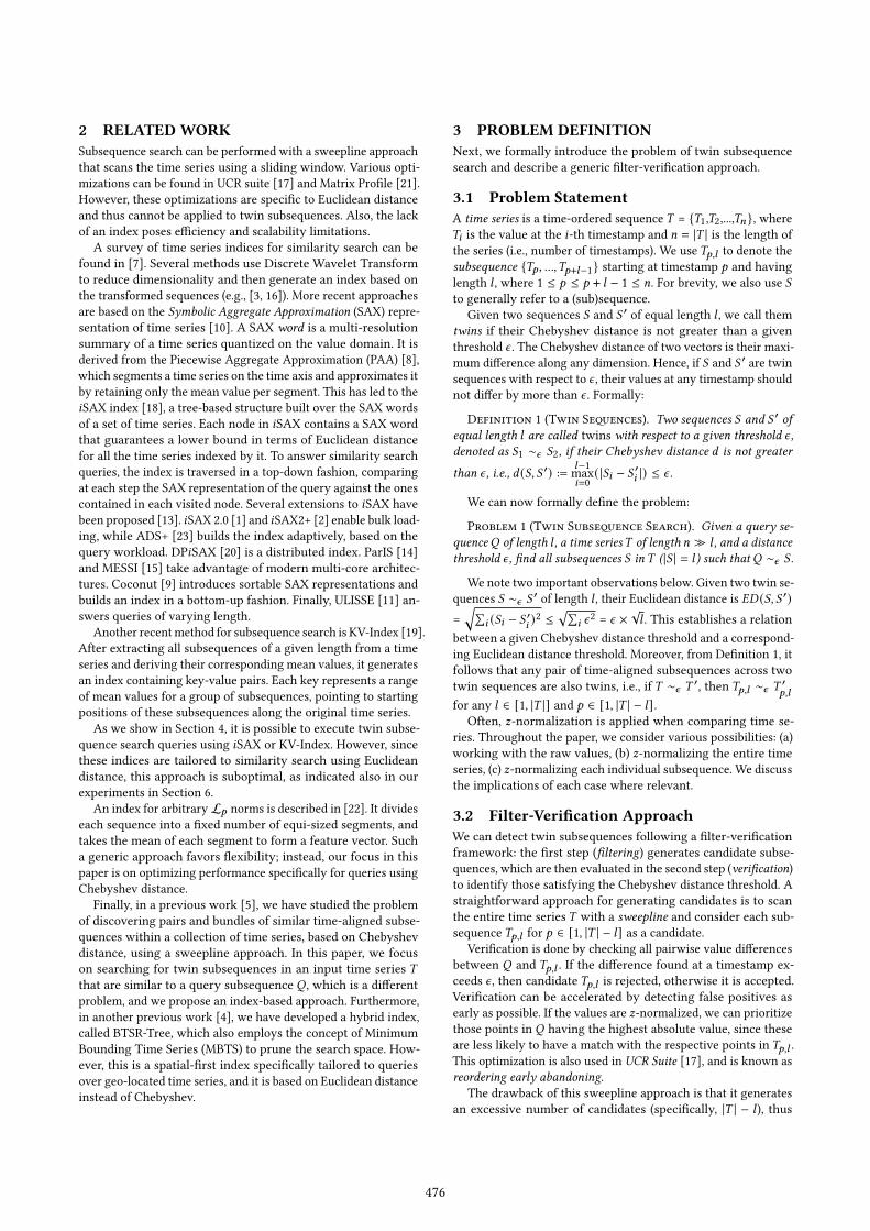
3 PROBLEM DEFINITIONNext, we formally introduce the problem of twin subsequence
search and describe a generic filter-verification approach.
3.1 Problem StatementA time series is a time-ordered sequence 𝑇 = {𝑇1,𝑇2,...,𝑇𝑛}, where𝑇𝑖 is the value at the 𝑖-th timestamp and 𝑛 = |𝑇 | is the length of
the series (i.e., number of timestamps). We use 𝑇𝑝,𝑙 to denote the
subsequence {𝑇𝑝 , ...,𝑇𝑝+𝑙−1} starting at timestamp 𝑝 and having
length 𝑙 , where 1 ≤ 𝑝 ≤ 𝑝 + 𝑙 − 1 ≤ 𝑛. For brevity, we also use 𝑆
to generally refer to a (sub)sequence.
Given two sequences 𝑆 and 𝑆 ′ of equal length 𝑙 , we call themtwins if their Chebyshev distance is not greater than a given
threshold 𝜖 . The Chebyshev distance of two vectors is their maxi-
mum difference along any dimension. Hence, if 𝑆 and 𝑆 ′ are twinsequences with respect to 𝜖 , their values at any timestamp should
not differ by more than 𝜖 . Formally:
Definition 1 (Twin Seqences). Two sequences 𝑆 and 𝑆 ′ ofequal length 𝑙 are called twins with respect to a given threshold 𝜖 ,denoted as 𝑆1 ∼𝜖 𝑆2, if their Chebyshev distance 𝑑 is not greater
than 𝜖 , i.e., 𝑑 (𝑆, 𝑆 ′) := 𝑙−1max
𝑖=0( |𝑆𝑖 − 𝑆 ′𝑖 |) ≤ 𝜖 .
We can now formally define the problem:
Problem 1 (Twin Subseqence Search). Given a query se-quence𝑄 of length 𝑙 , a time series𝑇 of length 𝑛 ≫ 𝑙 , and a distancethreshold 𝜖 , find all subsequences 𝑆 in𝑇 (|𝑆 | = 𝑙) such that 𝑄 ∼𝜖 𝑆 .
We note two important observations below. Given two twin se-
quences 𝑆 ∼𝜖 𝑆 ′ of length 𝑙 , their Euclidean distance is 𝐸𝐷 (𝑆, 𝑆 ′)=
√∑𝑖 (𝑆𝑖 − 𝑆 ′𝑖 )2 ≤
√∑𝑖 𝜖
2= 𝜖 ×
√𝑙 . This establishes a relation
between a given Chebyshev distance threshold and a correspond-
ing Euclidean distance threshold. Moreover, from Definition 1, it
follows that any pair of time-aligned subsequences across two
twin sequences are also twins, i.e., if 𝑇 ∼𝜖 𝑇 ′, then 𝑇𝑝,𝑙 ∼𝜖 𝑇 ′𝑝,𝑙for any 𝑙 ∈ [1, |𝑇 |] and 𝑝 ∈ [1, |𝑇 | − 𝑙].
Often, 𝑧-normalization is applied when comparing time se-
ries. Throughout the paper, we consider various possibilities: (a)
working with the raw values, (b) 𝑧-normalizing the entire time
series, (c) 𝑧-normalizing each individual subsequence. We discuss
the implications of each case where relevant.
3.2 Filter-Verification ApproachWe can detect twin subsequences following a filter-verification
framework: the first step (filtering) generates candidate subse-quences, which are then evaluated in the second step (verification)to identify those satisfying the Chebyshev distance threshold. A
straightforward approach for generating candidates is to scan
the entire time series 𝑇 with a sweepline and consider each sub-
sequence 𝑇𝑝,𝑙 for 𝑝 ∈ [1, |𝑇 | − 𝑙] as a candidate.Verification is done by checking all pairwise value differences
between 𝑄 and 𝑇𝑝,𝑙 . If the difference found at a timestamp ex-
ceeds 𝜖 , then candidate 𝑇𝑝,𝑙 is rejected, otherwise it is accepted.
Verification can be accelerated by detecting false positives as
early as possible. If the values are 𝑧-normalized, we can prioritize
those points in 𝑄 having the highest absolute value, since these
are less likely to have a match with the respective points in 𝑇𝑝,𝑙 .
This optimization is also used in UCR Suite [17], and is known as
reordering early abandoning.The drawback of this sweepline approach is that it generates
an excessive number of candidates (specifically, |𝑇 | − 𝑙), thus
476

incurring a prohibitive cost when dealing with long series. To
filter candidates more effectively, in the following sections we
present methods based on indexing the subsequences of 𝑇 . First,
we address the problem using state-of-the-art indices; then, we
introduce a novel index tailored to twin subsequence search.
4 TWIN SUBSEQUENCE SEARCHWITHEXISTING INDICES
Next, we focus on two representative state-of-the-art indices for
time series similarity search, namely KV-Index [19] and 𝑖SAX [2],
showing how they can be used for twin subsequence search
without altering their structure.
4.1 KV-IndexGiven a time series 𝑇 , KV-Index [19] is built by considering all
its subsequences of a pre-defined length 𝑙 . Each subsequence 𝑆 is
represented by a pair (𝑝, `), where 𝑝 is its starting position (i.e.,
timestamp) in𝑇 and ` is its mean value over the next 𝑙 timestamps.
KV-Index is an inverted index constructed over these pairs. Each
key is a range of mean values, whereas each inverted list entry
contains intervals of positions.
Twin subsequence search can be performed with KV-Index
based on the following observation. If two subsequences 𝑆 and
𝑆 ′ of length 𝑙 are twins with respect to 𝜖 , i.e., 𝑆 ∼𝜖 𝑆 ′, thentheir mean values ` and ` ′ cannot differ by more than 𝜖 , i.e.,
|`−` ′ | ≤ 𝜖 . Based on this, we can use a KV-Index built over a time
series 𝑇 to generate candidates for detecting twin subsequences.
Specifically, assume a query sequence𝑄 with mean value `𝑞 . The
candidate subsequences in 𝑇 are those included in the inverted
lists with keys [`𝑚𝑖𝑛, `𝑚𝑎𝑥 ], such that `𝑚𝑖𝑛 −𝜖 ≤ `𝑞 ≤ `𝑚𝑎𝑥 +𝜖 .Then, the obtained candidates must be verified to derive the final
results. Notice that this property is not effective if each individual
subsequence has been 𝑧-normalized, because then all mean values
are zero. Hence, KV-Index is applicable when working with raw
values or if the entire sequence is 𝑧-normalized.
4.2 𝑖SAX Index𝑖SAX is a tree index structure for time series similarity search [2].
Time series are 𝑧-normalized and indexed using their SymbolicAggregate approXimation (SAX) [18]. The SAX representation
of a series is derived in two steps. The first applies PiecewiseAggregate Approximation (PAA) [8], which splits the series in a
specified number𝑚 of segments and approximates each one with
the mean value over the corresponding time interval. The second
step applies quantization to assign each mean value to a discrete
SAX symbol. Hence, each SAX symbol𝑋 corresponds to a range of
mean values [`𝑋𝑚𝑖𝑛, `𝑋𝑚𝑎𝑥
). The SAX representation of a series
is a sequence of𝑚 SAX symbols (one symbol per segment), and is
called SAX word. Notice that, by default, SAX words are derived
using precomputed breakpoints that are selected assuming 𝑧-
normalized values; nevertheless, non-normalized values can also
be handled by adjusting the breakpoints accordingly.
Twin subsequence search can be enabled over 𝑖SAX by rea-
soning as follows. Assume two subsequences 𝑆 and 𝑆 ′ of length 𝑙 ,and their SAX representations 𝑆𝐴𝑋 (𝑆) = {𝑋1, 𝑋2, ..., 𝑋𝑚} and𝑆𝐴𝑋 (𝑆 ′) = {𝑋 ′
1, 𝑋 ′
2, ..., 𝑋 ′𝑚}. As we have observed earlier, (a) if
two sequences are twins with respect to a threshold 𝜖 , then the
difference between their mean values is also bounded by 𝜖 , and
(b) any pair of time-aligned segments across two twin sequences
are also twins. Combining these two properties, we can see that
if 𝑆 ∼𝜖 𝑆 ′, then for each pair of symbols 𝑋𝑖 and 𝑋 ′𝑖in the re-
spective SAX representations, the mean values denoted by these
symbols must not differ by more than 𝜖 . Hence, if 𝑆 ∼𝜖 𝑆 ′, then`𝑋𝑖𝑚𝑎𝑥
≥ `𝑋 ′𝑖𝑚𝑖𝑛− 𝜖 and `𝑋𝑖𝑚𝑖𝑛
≤ `𝑋 ′𝑖𝑚𝑎𝑥
+ 𝜖 for any 𝑖 ∈ [1,𝑚].Consequently, we can perform twin subsequence search using
𝑖SAX as follows. Given a time series 𝑇 , we construct an 𝑖SAX
index over all its 𝑙-length subsequences. Then, for a query se-
quence 𝑄 , we traverse the 𝑖SAX index starting from its root. At
each node, we check the SAX word of𝑄 against the SAX word of
that node, applying the property mentioned above. If the check
fails, the node and its subtree can be safely pruned; otherwise,
the search continues at the node’s children. Once a leaf node is
reached, and qualifies according to this check, all subsequences
indexed therein are retrieved as candidates for verification.
5 THE TS-INDEXAs discussed in Section 4, it is possible to use KV-Index or 𝑖SAX
to identify candidates for twin subsequence queries. However,
since these indices are not tailored to the matching criterion, they
tend to generate a large number of false positives, incurring a sig-
nificant verification cost, as confirmed in our experiments. In the
following, we introduce TS-Index, which is specifically designed
for twin subsequence search. First, we provide an overview of
its structure and explain how it is constructed. Then, we present
an algorithm to evaluate twin subsequence queries specifying a
distance threshold.
5.1 Index StructureThe core concept in TS-Index is that of Minimum Bounding TimeSeries (MBTS) [4]. An MBTS is a pair of sequences that fully
encloses a set of time series T by indicating the maximum and
minimum values at each timestamp. Figure 2a depicts an example
of an MBTS enclosing a set of four time series. Formally:
Definition 2 (MBTS). Given a set T of time series with equallength 𝑙 , its MBTS 𝐵 = (𝐵⊓, 𝐵⊔) consists of an upper bounding
time series 𝐵⊓ and a lower bounding time series 𝐵⊔, constructedby respectively selecting the maximum and minimum values ateach timestamp 𝑖 ∈ {1, . . . , 𝑙} among all time series in T as follows:
𝐵⊓ = {max
𝑇 ∈T𝑇1, . . . ,max
𝑇 ∈T𝑇𝑙 }
𝐵⊔ = {min
𝑇 ∈T𝑇1, . . . ,min
𝑇 ∈T𝑇𝑙 }
(1)
The TS-Index has a tree structure. Each internal node points
to a set of children nodes, whereas each leaf node points to a
set of subsequences (more specifically, to the starting positions
of its indexed subsequences along the input time series 𝑇 ). All
leaf nodes are at the same level. Each node is associated with an
MBTS, which encloses all the sequences indexed therein. Clearly,
MBTS get tighter when descending from the root to the leaf
level. Figure 3a illustrates an example of TS-Index for nine input
sequences. The MBTS of each node is depicted as a grey band.
5.2 Index ConstructionAssume an input time series 𝑇 and a subsequence length 𝑙 . The
TS-Index over𝑇 is constructed in a top-down fashion, by sequen-
tially inserting all 𝑙-length subsequences of 𝑇 . When inserting
a sequence 𝑆 , we traverse the index from the root, selecting at
each level the node whose MBTS has the smallest distance from
𝑆 , until a leaf node is reached. The distance between a sequence
𝑆 and an MBTS 𝐵 is calculated using the following formula:
477
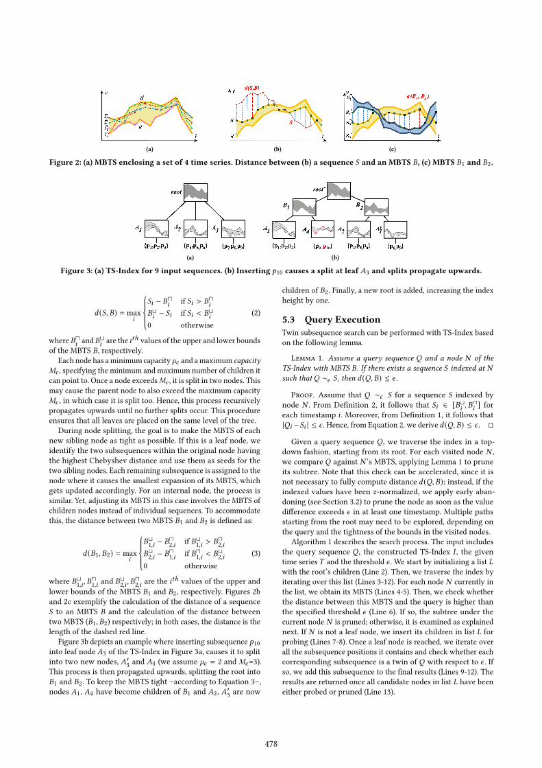
(a) (b) (c)
Figure 2: (a) MBTS enclosing a set of 4 time series. Distance between (b) a sequence 𝑆 and an MBTS 𝐵, (c) MBTS 𝐵1 and 𝐵2.
(a) (b)
Figure 3: (a) TS-Index for 9 input sequences. (b) Inserting 𝑝10 causes a split at leaf 𝐴3 and splits propagate upwards.
𝑑 (𝑆, 𝐵) = max
𝑖
𝑆𝑖 − 𝐵⊓𝑖 if 𝑆𝑖 > 𝐵⊓
𝑖
𝐵⊔𝑖− 𝑆𝑖 if 𝑆𝑖 < 𝐵⊔
𝑖
0 otherwise
(2)
where𝐵⊓𝑖and𝐵⊔
𝑖are the 𝑖𝑡ℎ values of the upper and lower bounds
of the MBTS 𝐵, respectively.
Each node has aminimum capacity `𝑐 and amaximum capacity𝑀𝑐 , specifying the minimum and maximum number of children it
can point to. Once a node exceeds𝑀𝑐 , it is split in two nodes. This
may cause the parent node to also exceed the maximum capacity
𝑀𝑐 , in which case it is split too. Hence, this process recursively
propagates upwards until no further splits occur. This procedure
ensures that all leaves are placed on the same level of the tree.
During node splitting, the goal is to make the MBTS of each
new sibling node as tight as possible. If this is a leaf node, we
identify the two subsequences within the original node having
the highest Chebyshev distance and use them as seeds for the
two sibling nodes. Each remaining subsequence is assigned to the
node where it causes the smallest expansion of its MBTS, which
gets updated accordingly. For an internal node, the process is
similar. Yet, adjusting its MBTS in this case involves the MBTS of
children nodes instead of individual sequences. To accommodate
this, the distance between two MBTS 𝐵1 and 𝐵2 is defined as:
𝑑 (𝐵1, 𝐵2) = max
𝑖
𝐵⊔1,𝑖− 𝐵⊓
2,𝑖if 𝐵⊔
1,𝑖> 𝐵⊓
2,𝑖
𝐵⊔2,𝑖− 𝐵⊓
1,𝑖if 𝐵⊓
1,𝑖< 𝐵⊔
2,𝑖
0 otherwise
(3)
where 𝐵⊔1,𝑖, 𝐵⊓
1,𝑖and 𝐵⊔
2,𝑖, 𝐵⊓
2,𝑖are the 𝑖𝑡ℎ values of the upper and
lower bounds of the MBTS 𝐵1 and 𝐵2, respectively. Figures 2b
and 2c exemplify the calculation of the distance of a sequence
𝑆 to an MBTS 𝐵 and the calculation of the distance between
two MBTS (𝐵1, 𝐵2) respectively; in both cases, the distance is the
length of the dashed red line.
Figure 3b depicts an example where inserting subsequence 𝑝10into leaf node 𝐴3 of the TS-Index in Figure 3a, causes it to split
into two new nodes, 𝐴′3and 𝐴4 (we assume `𝑐 = 2 and 𝑀𝑐=3).
This process is then propagated upwards, splitting the root into
𝐵1 and 𝐵2. To keep the MBTS tight –according to Equation 3–,
nodes 𝐴1, 𝐴4 have become children of 𝐵1 and 𝐴2, 𝐴′3are now
children of 𝐵2. Finally, a new root is added, increasing the index
height by one.
5.3 Query ExecutionTwin subsequence search can be performed with TS-Index based
on the following lemma.
Lemma 1. Assume a query sequence 𝑄 and a node 𝑁 of theTS-Index with MBTS 𝐵. If there exists a sequence 𝑆 indexed at 𝑁such that 𝑄 ∼𝜖 𝑆 , then 𝑑 (𝑄, 𝐵) ≤ 𝜖 .
Proof. Assume that 𝑄 ∼𝜖 𝑆 for a sequence 𝑆 indexed by
node 𝑁 . From Definition 2, it follows that 𝑆𝑖 ∈ [𝐵⊔𝑖 , 𝐵⊓𝑖] for
each timestamp 𝑖 . Moreover, from Definition 1, it follows that
|𝑄𝑖 −𝑆𝑖 | ≤ 𝜖 . Hence, from Equation 2, we derive 𝑑 (𝑄, 𝐵) ≤ 𝜖 . □
Given a query sequence 𝑄 , we traverse the index in a top-
down fashion, starting from its root. For each visited node 𝑁 ,
we compare 𝑄 against 𝑁 ’s MBTS, applying Lemma 1 to prune
its subtree. Note that this check can be accelerated, since it is
not necessary to fully compute distance 𝑑 (𝑄, 𝐵); instead, if theindexed values have been 𝑧-normalized, we apply early aban-
doning (see Section 3.2) to prune the node as soon as the value
difference exceeds 𝜖 in at least one timestamp. Multiple paths
starting from the root may need to be explored, depending on
the query and the tightness of the bounds in the visited nodes.
Algorithm 1 describes the search process. The input includes
the query sequence 𝑄 , the constructed TS-Index 𝐼 , the given
time series 𝑇 and the threshold 𝜖 . We start by initializing a list 𝐿
with the root’s children (Line 2). Then, we traverse the index by
iterating over this list (Lines 3-12). For each node 𝑁 currently in
the list, we obtain its MBTS (Lines 4-5). Then, we check whether
the distance between this MBTS and the query is higher than
the specified threshold 𝜖 (Line 6). If so, the subtree under the
current node 𝑁 is pruned; otherwise, it is examined as explained
next. If 𝑁 is not a leaf node, we insert its children in list 𝐿 for
probing (Lines 7-8). Once a leaf node is reached, we iterate over
all the subsequence positions it contains and check whether each
corresponding subsequence is a twin of 𝑄 with respect to 𝜖 . If
so, we add this subsequence to the final results (Lines 9-12). The
results are returned once all candidate nodes in list 𝐿 have been
either probed or pruned (Line 13).
478

Algorithm 1: TwinSubsequenceSearchInput :Time series𝑇 , TS-Index 𝐼 , query𝑄 , threshold 𝜖
Output :List 𝑅 of twin subsequences to𝑄
1 𝑅 ← ∅2 𝐿 ← 𝐼 .𝑟𝑜𝑜𝑡 .getChildren()3 while 𝐿 ≠ ∅ do4 𝑁 ← 𝐿.getNext()5 𝐵 ← 𝑁 .𝑀𝐵𝑇𝑆
6 if d( (𝑄, 𝐵) ≤ 𝜖 then7 if 𝑁 is not leaf then8 𝐿 ← 𝐿 ∪ {𝑁 .getChildren() }9 else10 foreach 𝑝 ∈ 𝑁 .getPositions() do11 if d( (𝑄,𝑇𝑝,𝑙 ) ≤ 𝜖 then12 𝑅 ← 𝑅 ∪𝑇𝑝,𝑙
13 return R
Table 1: Datasets and distance thresholds.Dataset 𝒏 𝝐 (norm) 𝝐 (non-norm)Insect 64,436 0.5,0.75,1,1.25,1.5 50, 100,150,200,250EEG 1,801,999 0.1,0.2,0.3,0.4,0.5 20, 40,60,80,100
Table 2: Other parameters.Parameter ValueNumber𝑚 of segments 5, 10, 20, 25, 50Sequence length 𝑙 50, 100, 150, 200, 250
6 EXPERIMENTAL EVALUATIONNext, we present an experimental evaluation of our methods
against two real-world datasets.
6.1 Experimental SetupWe performed experiments against two real-world time series
(see Table 1), which contain diverse patterns and differ in their
total duration. In particular, the Insect Movement [12] series
contains 64,436 insect telemetry readings spanning around 30
minutes (36 readings/sec), whereas the Electroencephalography(EEG) [12] series comprises 1,801,999 EEG readings at 500Hz last-
ing one hour. Unless stated otherwise, we 𝑧-normalize the time
series to facilitate selection of distance thresholds.
Table 1 indicates the different values for the distance threshold
𝜖 used in the experiments against each dataset, for 𝑧-normalized
(norm) or original values (non-norm). Table 2 contains the values
for subsequence length 𝑙 and number of segments𝑚, which are
common in the experiments on both datasets. In both tables,
default values are in bold. These values have been selected after
running several preliminary tests, which also guided selection
of other parameters. Specifically, for 𝑖SAX, the maximum node
capacity is set to 10,000 to enable index construction in reasonable
time even for larger datasets. The default values for minimum
and maximum node capacity in TS-Index are set to `𝑐 = 10 and
𝑀𝑐 = 30, respectively.
For each dataset, we randomly picked 100 subsequences, each
of length 𝑙 = 100 points, and used them as the query workload in
all tests against that dataset. We report average response time per
query (in milliseconds). We implemented all methods, including
KV-Index, 𝑖SAX, and TS-Index, in Java. In all implementations,
the structure of the index is kept in memory, while the original
input dataset is stored on disk. Leaf nodes in the index contain
the starting positions of the subsequences in the input time series.
Thus, when a leaf is reached at query time, its corresponding
subsequences are obtained from the input time series file using
random access. All experiments were conducted on a server with
(a) Insect Dataset (b) EEG Dataset
Figure 4: Varying distance threshold 𝜖.
(a) Insect Dataset (b) EEG Dataset
Figure 5: Varying subsequence length 𝑙 .
(a) Insect Dataset (b) EEG Dataset
Figure 6: Varying 𝜖 on 𝑧-normalized subsequences.
4 CPUs, each equipped with 8 cores clocked at 2.13GHz, and 256
GB RAM running Debian Linux.
6.2 PerformanceWe compare the average execution time per query for varying
values of each parameter, setting the rest to their default values.
6.2.1 Varying threshold 𝜖 . Figure 4 depicts query execution
time (in logarithmic scale) for varying threshold 𝜖 . As expected,
searching with the Sweepline approach has a fixed cost per
dataset regardless of 𝜖 , since it needs to scan all subsequences ex-
tracted from the input time series. Relaxing the threshold incurs
an overhead when an index is involved. Queries against KV-Index
perform poorly compared to other indices, since filtering based
on mean values achieves less pruning. Searching with TS-Index
outperforms the rest in every setting for both tested datasets.
Overall, TS-Index is at least an order of magnitude more effi-
cient in twin subsequence search compared to the KV-Index and
Sweepline approaches. It is also consistently better than 𝑖SAX as
it is less susceptible to fluctuations in the input sequences.
6.2.2 Varying Subsequence Length. Figure 5 plots performance
results with a varying length 𝑙 for subsequences obtained from
the input time series. Increasing 𝑙 seems to slightly negatively
affect all approaches, except for TS-Index. Since longer subse-
quences are extracted, more checks are required, both in nodes (in
case of 𝑖SAX) and raw subsequences during verification. Instead,
TS-Index is faster when longer subsequences are specified, as it
becomes less likely to findmatching twins. In particular, TS-Index
has higher pruning capability and can skip non-qualifying sub-
trees earlier at higher levels in the tree hierarchy. Thus, fewer
479

(a) Insect Dataset (b) EEG Dataset
Figure 7: Varying 𝜖 on non-normalized data.
(a) Memory Footprint (b) Build Time
Figure 8: Memory footprint and build time per index.
leaf nodes are accessed and need to be verified, saving much of
the verification cost for checks per timestamp.
6.2.3 Searching over 𝑧-normalized subsequences. We repeat
the experiment for varying distance threshold 𝜖 , this time apply-
ing 𝑧-normalization over each individual subsequence, before in-
serting it in the index. As mentioned in Section 4.1, KV-Index can-
not be built on such data since the mean value per subsequence
would always be zero; thus, we only compare TS-Index with
𝑖SAX. The results are depicted in Figure 6. Clearly, 𝑧-normalizing
the subsequences separately has no significant effect on the per-
formance of TS-Index; the results are similar to those in Figure 4,
with TS-Index outperforming 𝑖SAX in all cases.
6.2.4 Searching on Non-Normalized Data. Query execution
cost for identifying twin subsequences against the raw (non-
normalized) time series is depicted in Figure 7. Overall, TS-Index
copes better than all the rest even for raw data, confirming its
suitability for twin subsequence search in various settings.
6.2.5 Index Size. Figure 8a presents the memory footprint of
TS-Index, 𝑖SAX and KV-Index for each dataset. KV-Index requires
less space than TS-Index and 𝑖SAX, as it only keeps in memory
the mean value and position range per subsequence. Instead,
TS-Index and 𝑖SAX occupy more space due to their more complex
structures. Specifically, 𝑖SAX requires two to three times less
space than TS-Index. Indeed, 𝑖SAX needs to store one SAX word
per node, whereas a node in TS-Index is represented by an MBTS,
hence its increased memory footprint. Nevertheless, all indices,
including TS-Index, have sizes that easily fit in main memory.
6.2.6 Build Time. Similarly to the index size, and due to the
significantly less required calculations (i.e., only subsequence
mean values need be calculated and no node splitting is needed),
KV-Index requires significantly less time to be constructed than
𝑖SAX and TS-Index (Figure 8b). 𝑖SAX is the slowest index to
be built, since it needs to additionally convert the PAA of each
subsequence to a SAX word for each extracted subsequence.
7 CONCLUSIONSIn this paper, we have introduced the twin subsequence search
problem. Given a query sequence 𝑄 , an input time series 𝑇 and
a distance threshold 𝜖 , this task retrieves all subsequences in
𝑇 with Chebyshev distance to 𝑄 not higher than 𝜖 . To answer
this query efficiently, we have introduced the TS-Index. We have
described the index structure and proposed algorithms for effi-
cient index construction and query answering. Our experimental
evaluation assesses the TS-Index in terms of construction cost
and confirms its superiority for twin subsequence search queries
when compared to the state-of-the-art.
ACKNOWLEDGMENTSThis work was supported by the EU H2020 project SmartData-
Lake (825041), the EU H2020 project OpertusMundi (870228) and
the NSRF 2014-2020 project HELIX (5002781).
REFERENCES[1] Alessandro Camerra, Themis Palpanas, Jin Shieh, and Eamonn J. Keogh. 2010.
iSAX 2.0: Indexing and Mining One Billion Time Series. In ICDM. 58–67.
[2] Alessandro Camerra, Jin Shieh, Themis Palpanas, Thanawin Rakthanmanon,
and Eamonn J. Keogh. 2014. Beyond one billion time series: indexing and
mining very large time series collections with i SAX2+. Knowl. Inf. Syst. 39, 1(2014), 123–151.
[3] Kin-pong Chan and Ada Wai-Chee Fu. 1999. Efficient Time Series Matching
by Wavelets. In ICDE. 126–133.[4] Georgios Chatzigeorgakidis, Dimitrios Skoutas, Kostas Patroumpas, Spiros
Athanasiou, and Spiros Skiadopoulos. 2017. Indexing Geolocated Time Series
Data. In SIGSPATIAL. 19:1–19:10.[5] Georgios Chatzigeorgakidis, Dimitrios Skoutas, Kostas Patroumpas, Themis
Palpanas, Spiros Athanasiou, and Spiros Skiadopoulos. 2019. Local pair and
bundle discovery over co-evolving time series. In SSTD. 160–169.[6] Hui Ding, Goce Trajcevski, Peter Scheuermann, Xiaoyue Wang, and Eamonn
Keogh. 2008. Querying and mining of time series data: experimental com-
parison of representations and distance measures. Proceedings of the VLDBEndowment 1, 2 (2008), 1542–1552.
[7] Karima Echihabi, Kostas Zoumpatianos, Themis Palpanas, and Houda Ben-
brahim. 2018. The Lernaean Hydra of Data Series Similarity Search: An
Experimental Evaluation of the State of the Art. PVLDB 12, 2 (2018), 112–127.
[8] Eamonn J. Keogh, Kaushik Chakrabarti, Michael J. Pazzani, and Sharad Mehro-
tra. 2001. Dimensionality Reduction for Fast Similarity Search in Large Time
Series Databases. Knowl. Inf. Syst. 3, 3 (2001), 263–286.[9] Haridimos Kondylakis, Niv Dayan, Kostas Zoumpatianos, and Themis Pal-
panas. 2018. Coconut: A scalable bottom-up approach for building data series
indexes. PVLDB 11, 6 (2018), 677–690.
[10] Jessica Lin, Eamonn J. Keogh, Li Wei, and Stefano Lonardi. 2007. Experiencing
SAX: a novel symbolic representation of time series. Data Min. Knowl. Discov.15, 2 (2007), 107–144.
[11] Michele Linardi and Themis Palpanas. 2020. Scalable Data Series Subsequence
Matching with ULISSE. VLDBJ 11, 13 (2020), 2236–2248.[12] Abdullah Mueen, Eamonn Keogh, Qiang Zhu, Sydney Cash, and Brandon
Westover. 2009. Exact discovery of time series motifs. In SIAM. 473–484.
[13] Themis Palpanas. 2020. Evolution of a Data Series Index. CCIS 1197 (2020).[14] Botao Peng, Panagiota Fatourou, and Themis Palpanas. 2018. ParIS: The
Next Destination for Fast Data Series Indexing and Query Answering. In IEEEBigData.
[15] Botao Peng, Panagiota Fatourou, and Themis Palpanas. 2020. MESSI: In-
Memory Data Series Indexing. In ICDE. 337–348.[16] Ivan Popivanov and Renée J. Miller. 2002. Similarity Search Over Time-Series
Data Using Wavelets. In ICDE. 212–221.[17] Thanawin Rakthanmanon, Bilson Campana, AbdullahMueen, Gustavo Batista,
BrandonWestover, Qiang Zhu, Jesin Zakaria, and EamonnKeogh. 2012. Search-
ing and mining trillions of time series subsequences under dynamic time
warping. In SIGKDD. 262–270.[18] Jin Shieh and Eamonn J. Keogh. 2008. iSAX: indexing and mining terabyte
sized time series. In SIGKDD. 623–631.[19] Jiaye Wu, Peng Wang, Ningting Pan, Chen Wang, Wei Wang, and Jianmin
Wang. 2019. KV-Match: A Subsequence Matching Approach Supporting
Normalization and Time Warping. In ICDE. 866–877.[20] Djamel Edine Yagoubi, Reza Akbarinia, Florent Masseglia, and Themis Pal-
panas. 2020. Massively Distributed Time Series Indexing and Querying. IEEETrans. Knowl. Data Eng. 32, 1 (2020), 108–120.
[21] Chin-Chia Michael Yeh, Yan Zhu, Liudmila Ulanova, Nurjahan Begum, Yifei
Ding, Hoang Anh Dau, Diego Furtado Silva, Abdullah Mueen, and Eamonn
Keogh. 2016. Matrix profile I: all pairs similarity joins for time series: a unifying
view that includes motifs, discords and shapelets. In ICDM.
[22] Byoung-Kee Yi and Christos Faloutsos. 2000. Fast Time Sequence Indexing
for Arbitrary Lp Norms. In VLDB. 385–394.[23] Kostas Zoumpatianos, Stratos Idreos, and Themis Palpanas. 2014. Indexing
for interactive exploration of big data series. In SIGMOD. 1555–1566.
480

![Twin Subsequence Search in Time Serieshelios.mi.parisdescartes.fr/~themisp/publications/edbt21-twinsubsequences.pdfin certain datasets [6, 22]. In this work, we use the Chebyshev distance](https://img.pdfslide.net/doc/110x75/610a9723b38465445c35550f/twin-subsequence-search-in-time-themisppublicationsedbt21-twinsubsequencespdf.jpg)