arX

iv:1

403.

5226

v2 [

hep-

ph]

1 J

ul 2

014

Twist-2 Generalized TMDs and the Spin/Orbital Structure

of the Nucleon

K. Kanazawa1,2, C. Lorce3, A. Metz2, B. Pasquini4, M. Schlegel5

1 Graduate School of Science and Technology,

Niigata University, Ikarashi, Niigata 950-2181, Japan

2Department of Physics, Barton Hall, Temple University, Philadelphia, PA 19122, USA

3 IPNO, Universite Paris-Sud, CNRS/IN2P3, 91406 Orsay, France and

IFPA, AGO Department, Universite de Liege, Sart-Tilman, 4000 Liege, Belgium

4Dipartimento di Fisica, Universita degli Studi di Pavia, and

Istituto Nazionale di Fisica Nucleare, Sezione di Pavia, I-27100 Pavia, Italy

5Institute for Theoretical Physics, Tubingen University,

Auf der Morgenstelle 14, D-72076 Tubingen, Germany

Abstract

Generalized transverse-momentum dependent parton distributions (GTMDs) encode the most

general parton structure of hadrons. Here we focus on two twist-2 GTMDs which are denoted

by F1,4 and G1,1 in parts of the literature. As already shown previously, both GTMDs have a

close relation to orbital angular momentum of partons inside a hadron. However, recently even the

mere existence of F1,4 and G1,1 has been doubted. We explain why this claim does not hold. We

support our model-independent considerations by calculating the two GTMDs in the scalar diquark

model and in the quark-target model, where we also explicitly check the relation to orbital angular

momentum. In addition, we compute F1,4 and G1,1 at large transverse momentum in perturbative

Quantum Chromodynamics and show that they are nonzero.

PACS numbers: 12.39.-x, 13.88.+e, 13.60.Hb, 12.38.-t

1

I. INTRODUCTION

During the past two decades, a lot of attention has been paid to generalized parton

distributions (GPDs) [1–7] and to transverse-momentum dependent parton distributions

(TMDs) [8–12]. Those objects are of particular interest because they describe the three-

dimensional parton structure of hadrons — the distribution of the parton’s longitudinal

momentum and transverse position in the case of GPDs, and the distribution of the parton’s

longitudinal momentum and transverse momentum in the case of TMDs. Even though GPDs

and TMDs already are quite general entities, the maximum possible information about

the (two-) parton structure of strongly interacting systems is encoded in GTMDs [13–15].

GTMDs can reduce to GPDs and to TMDs in certain kinematical limits, and therefore

they are often denoted as mother distributions. The Fourier transform of GTMDs can be

considered as Wigner distributions [16–18], the quantum-mechanical analogue of classical

phase-space distributions.

A classification of GTMDs for quarks (through twist-4) for a spin-0 target was given

in Ref. [13], followed by a corresponding work for a spin-12target [14]. In Ref. [15], the

counting of quark GTMDs was independently confirmed, and a complete classification of

gluon GTMDs was provided as well. GTMDs were computed in spectator models [13, 14],

and in two different light-front quark models [18, 19]. Gluon GTMDs quite naturally appear

when describing high-energy diffractive processes like vector meson production or Higgs

production in so-called kT -factorization in Quantum Chromodynamics (QCD) [20–22]. It

is important to note that, in general, there exists no argument according to which, as a

matter of principle, GTMDs cannot be measured, even though for quark GTMDs a proper

high-energy process has yet to be identified.

Recent developments revealed an intimate connection between two specific GTMDs —

denoted by F1,4 and G1,1 in Ref. [14] — and the spin/orbital structure of the nucleon. (See

Refs. [23, 24] for recent reviews on the decomposition of the nucleon spin.) In particular,

the relation between F1,4 and the orbital angular momentum (OAM) of partons inside a

longitudinally polarized nucleon [18, 25–28] has already attracted considerable attention.

As shown in [18], this relation gets its most intuitive meaning when expressed in terms of

the Wigner function F1,4, i.e., the Fourier transform of F1,4. It is also quite interesting that,

depending on how one chooses the path of the gauge link that makes the GTMD correlator

2

gauge invariant [27, 28], F1,4 provides either the (canonical) OAM of Jaffe-Manohar [29] or

the OAM in the definition of Ji [2]. (We also refer to [30] for a closely related discussion.)

The connection between OAM and F1,4 could make the canonical OAM accessible to Lattice

QCD as first pointed out in [25]. The GTMD G1,1 can be considered as “partner” of F1,4

as it describes longitudinally polarized partons in an unpolarized nucleon [18, 31]. The very

close analogy between those two functions becomes most transparent if one speaks in terms

of spin-orbit correlations [31]. While F1,4 quantifies the correlation between the nucleon spin

and the OAM of partons, G1,1 quantifies the correlation between the parton spin and the

OAM of partons [31].

Despite all those developments, recently it has been argued that OAM of partons cannot

be explored through leading-twist GTMDs [32, 33]. In fact, the mere existence of F1,4 and

G1,1 has been doubted. Here we refute this criticism and explain why the arguments given

in [32, 33] do not hold. A key problem of the work in [32, 33] is the application of a two-body

scattering picture for the classification of GTMDs, which turns out to be too restrictive. In

order to make as clear as possible that in general neither F1,4 nor G1,1 vanish, we also

compute them in the scalar diquark model of the nucleon, in the quark-target model, and

in perturbative QCD for large transverse parton momenta. In addition, for the two models,

we show explicitly the connection between the two GTMDs and the OAM of partons. The

model calculations are carried out in standard perturbation theory for correlation functions,

and also by using the overlap representation in terms of light-front wave functions (LFWFs)

where some of the results become rather intuitive.

The paper is organized as follows: In Sect. II we specify our conventions and repeat some

key ingredients for the counting of GTMDs, while Sect. III essentially deals with our reply

to the arguments given in [32, 33]. The calculations of F1,4 and G1,1 in the scalar diquark

model and in the quark-target model are discussed in Sect. IV, along with their relation to

OAM of partons. In Sect. V we repeat the studies of Sect. IV by making use of LFWFs.

The computation of the two GTMDs at large transverse momentum is presented in Sect. VI.

We summarize the paper in Sect. VII.

II. DEFINITION OF GTMDS

In this section we review the definition of the GTMDs for quarks, which have been

3

classified in Refs. [13, 14] and further discussed also for the gluon sector in Ref. [15]. We

begin by introducing two light-like four-vectors n± satisfying n2± = 0 and n+ ·n− = 1. They

allow one to decompose a generic four-vector aµ as

a = a+n+ + a−n− + a⊥, (1)

where the transverse light-front four-vector is defined as aµ⊥ = gµν⊥ aν , with gµν⊥ = gµν −nµ+n

ν− − nµ

−nν+. We consider the following fully-unintegrated quark-quark correlator

W[Γ]Λ′Λ(P, k,∆, n−; η) =

1

2

∫

d4z

(2π)4eik·z 〈p′,Λ′|T{ψ(−z

2)ΓWn−

ψ( z2)}|p,Λ〉, (2)

which depends on the initial (final) hadron light-front helicity Λ (Λ′), and the following

independent four-vectors:

• the average nucleon four-momentum P = 12(p′ + p);

• the average quark four-momentum k = 12(k′ + k);

• the four-momentum transfer ∆ = p′ − p = k′ − k;

• the light-like four-vector n−.

The object Γ in Eq. (2) stands for any element of the basis {1, γ5, γµ, γµγ5, iσµνγ5} in Dirac

space. The Wilson contour Wn−≡ W(−z

2, z2|ηn−) ensures the color gauge invariance of the

correlators, connecting the points −z2and z

2via the intermediate points −z

2+ η∞n− and

z2+ η∞n−. The parameter η = ± indicates whether the Wilson contour is future-pointing

or past-pointing. The four-vector n− defines the light-front direction which allows one to

organize the structure of the correlator as an expansion in(

MP+

)t−2, where t defines the

operational twist [34]. Without loss of generality, we choose the z-axis along the ~n+ =

−~n− direction, i.e., n− = 1√2(1, 0, 0,−1) and n+ = 1√

2(1, 0, 0, 1). Therefore, the light-

front coordinates of a generic four-vector a = [a+, a−,a⊥] are given by a+ = 1√2(a0 + a3),

a− = 1√2(a0 − a3), and a⊥ = (a1, a2).

Since the light-front quark energy is hard to measure, one can focus on the k−-integrated

version of Eq. (2),

W[Γ]Λ′Λ(P, x, k⊥,∆, n−; η) =

1

2

∫

dk−∫

d4z

(2π)4eik·z 〈p′,Λ′|ψ(−z

2)ΓWn−

ψ( z2)|p,Λ〉, (3)

where time-ordering is not needed anymore and k = [xP+, k−, k⊥]. The functions that

parametrize this correlator are called GTMDs and can be seen as the mother distributions

of GPDs and TMDs [13–15].

4

A. Helicity Amplitudes and GTMD Counting

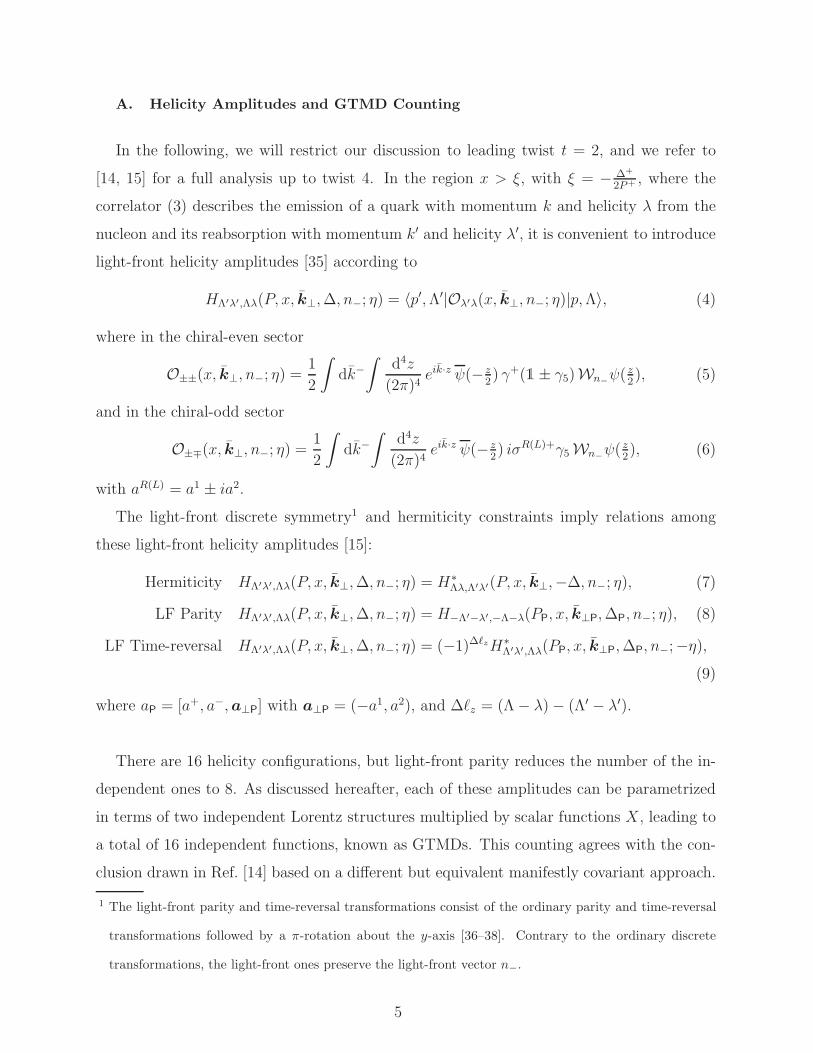
In the following, we will restrict our discussion to leading twist t = 2, and we refer to

[14, 15] for a full analysis up to twist 4. In the region x > ξ, with ξ = − ∆+

2P+ , where the

correlator (3) describes the emission of a quark with momentum k and helicity λ from the

nucleon and its reabsorption with momentum k′ and helicity λ′, it is convenient to introduce

light-front helicity amplitudes [35] according to

HΛ′λ′,Λλ(P, x, k⊥,∆, n−; η) = 〈p′,Λ′|Oλ′λ(x, k⊥, n−; η)|p,Λ〉, (4)

where in the chiral-even sector

O±±(x, k⊥, n−; η) =1

2

∫

dk−∫

d4z

(2π)4eik·z ψ(−z

2) γ+(1± γ5)Wn−

ψ( z2), (5)

and in the chiral-odd sector

O±∓(x, k⊥, n−; η) =1

2

∫

dk−∫

d4z

(2π)4eik·z ψ(−z

2) iσR(L)+γ5Wn−

ψ( z2), (6)

with aR(L) = a1 ± ia2.

The light-front discrete symmetry1 and hermiticity constraints imply relations among

these light-front helicity amplitudes [15]:

Hermiticity HΛ′λ′,Λλ(P, x, k⊥,∆, n−; η) = H∗Λλ,Λ′λ′(P, x, k⊥,−∆, n−; η), (7)

LF Parity HΛ′λ′,Λλ(P, x, k⊥,∆, n−; η) = H−Λ′−λ′,−Λ−λ(PP, x, k⊥P,∆P, n−; η), (8)

LF Time-reversal HΛ′λ′,Λλ(P, x, k⊥,∆, n−; η) = (−1)∆ℓzH∗Λ′λ′,Λλ(PP, x, k⊥P,∆P, n−;−η),

(9)

where aP = [a+, a−,a⊥P] with a⊥P = (−a1, a2), and ∆ℓz = (Λ− λ)− (Λ′ − λ′).

There are 16 helicity configurations, but light-front parity reduces the number of the in-

dependent ones to 8. As discussed hereafter, each of these amplitudes can be parametrized

in terms of two independent Lorentz structures multiplied by scalar functions X , leading to

a total of 16 independent functions, known as GTMDs. This counting agrees with the con-

clusion drawn in Ref. [14] based on a different but equivalent manifestly covariant approach.

1 The light-front parity and time-reversal transformations consist of the ordinary parity and time-reversal

transformations followed by a π-rotation about the y-axis [36–38]. Contrary to the ordinary discrete

transformations, the light-front ones preserve the light-front vector n−.

5

Let us now explain why there are two GTMDs associated with each of the 8 independent

helicity amplitudes. The GTMDs can only depend on variables that are invariant under the

transformations which preserve the light-front vector n− up to a scaling factor, namely the

kinematic Lorentz transformations (the three light-front boosts and the rotations about the

z-axis) and the light-front parity transformation2. From the independent four-vectors at our

disposal, these variables are3 (x, ξ,κ2⊥,κ⊥ · D⊥,D

2⊥), where κ⊥ = k⊥ − xP⊥ and D⊥ =

∆⊥ + 2ξP⊥. By conservation of the total angular momentum along the z-direction, each

light-front helicity amplitude is associated with a definite OAM transfer ∆ℓz. Since there are

only two frame-independent (or intrinsic) transverse vectors available, the general structure

of a light-front helicity amplitude is given in terms of explicit global powers of κ⊥ and D⊥,

accounting for the OAM transfer, multiplied by a scalar function X(x, ξ,κ2⊥,κ⊥ ·D⊥,D

2⊥; η).

As explicitly discussed in Ref. [15], from two independent transverse vectors, one can form

only two independent Lorentz structures associated with a given ∆ℓz, or, equivalently, light-

front helicity amplitude.

B. GTMD Parametrization

Since the GTMD counting is frame-independent, we are free to work in any frame. For

convenience, we choose the symmetric frame where the momenta are given by

P =[

P+, P−, 0⊥]

,

k =[

xP+, k−, k⊥]

,

∆ =[

−2ξP+, 2ξP−,∆⊥]

(10)

with P− =M2+∆

2⊥/4

2(1−ξ2)P+ , and the intrinsic transverse vectors simply reduce to κ⊥ = k⊥ and

D⊥ = ∆⊥. Restricting ourselves to the chiral-even sector and using the parametrization in

Ref. [14], the light-front helicity amplitudes for ξ = 0, Λ′ = Λ = ± and λ′ = λ = ± read

HΛλ,Λλ = 12

[

F1,1 + ΛλG1,4 +i(k⊥×∆⊥)z

M2 (ΛF1,4 − λG1,1)]

. (11)

2 For convenience, we do not include light-front time-reversal at this stage. The counting then leads to

16 complex-valued GTMDs with no definite transformation properties under light-front time-reversal.

Including light-front time-reversal gives at the end 32 real-valued functions with definite transformation

properties. The parametrizations in Refs. [14, 15] have been chosen such that the real part of the GTMDs

is (naive) T-even and the imaginary part is (naive) T-odd.3 In general the GTMDs depend also on η.

6

Inverting this expression, we obtain for F1,4 and G1,1

i(k⊥×∆⊥)zM2 F1,4 =

12[H++,++ +H+−,+− −H−+,−+ −H−−,−−] , (12)

− i(k⊥×∆⊥)zM2 G1,1 =

12[H++,++ −H+−,+− +H−+,−+ −H−−,−−] . (13)

The function F1,4 describes how the longitudinal polarization of the target distorts the

unpolarized distribution of quarks, whereas G1,1 describes how the longitudinal polarization

of quarks distorts their distribution inside an unpolarized target [18].

III. THE TWO-BODY SCATTERING PICTURE

We are now in a position to address the criticism put forward in Refs. [32, 33]. In

these papers it has been argued that, based on parity arguments in a two-body scattering

picture, the functions F1,4 and G1,1 should not be included in a twist-2 parametrization.

This contradicts the findings of Refs. [13–15, 25] and the results obtained in explicit model

calculations [13, 14, 18, 26]. In the following, we will go along the arguments developed in

Refs. [32, 33] and explain why they actually do not hold. We note essentially three claims

in Refs. [32, 33] :

1. The Lorentz structure associated with the function F1,4 and appearing in the parametri-

zation of the correlator W[γ+]Λ′Λ in Ref. [14]

u(p′,Λ′)iσjkkj⊥∆

k⊥

M2u(p,Λ) ∝ 〈~SL · (~k⊥ × ~∆⊥)〉 (14)

is parity-odd. In the center-of-mass (CM) frame, or equivalently in the “lab” frame,

with the p-direction chosen as the z-direction, the net longitudinal polarization defined

in Eq. (14) is clearly a parity violating term (pseudoscalar) under space inversion. This

implies that a measurement of single longitudinal polarization asymmetries would

violate parity conservation in an ordinary two-body scattering process corresponding

to tree-level, twist-2 amplitudes.

2. As one can see from Eqs. (12) and (13), the functions F1,4 and G1,1 can be nonzero only

when the corresponding helicity amplitude combinations are imaginary. Hence, these

functions cannot have a straightforward partonic interpretation. Moreover, integrating

e.g. Eq. (12) over k⊥ gives zero, meaning that this term decouples from partonic

angular momentum sum rules.

7

3. In the CM frame, where the hadron and quark momenta are coplanar, there must be

another independent direction for the helicity amplitude combinations associated with

F1,4 andG1,1 to be non-zero. That is provided by twist-3 amplitudes and corresponding

GTMDs.

Let us first discuss the parity property of the Lorentz structure in Eq. (14). Parity is a

frame-independent symmetry, and so does not depend on any particular frame. Under an

ordinary parity transformation, see for instance Chapter 3.6 of Ref. [39], the structure in

Eq. (14) becomes

u(p′P,Λ′

P)iσjkkj⊥∆

k⊥

M2u(pP,ΛP), (15)

where ΛP and pP = (p0,−~p ) are the parity-transformed helicity and momentum. Clearly,

the structure (14) does not change sign under a parity transformation, and so is parity-

even4. This is consistent with the light-front helicity amplitudes given in Eq. (11), where

the structure (14) contributes in the form Λ i(k⊥×∆⊥)zM2 which is invariant under light-front

parity transformation. While it is true that the net longitudinal polarization SL = ~S· ~P/|~P | isparity-odd and therefore cannot generate by itself a parity-conserving single-spin asymmetry,

it is actually multiplied in Eq. (14) by (k⊥ ×∆⊥)z = (~k × ~∆) · ~P/|~P |, another parity-oddquantity which is related to the quark OAM. Therefore, the parity argument cannot be

used to exclude the possible connection between a single-spin asymmetry and the function

F1,4. The same is true for G1,1 using a similar argument where the nucleon polarization is

basically replaced by the quark polarization. We agree that longitudinal single-spin effects

for elastic two-body scattering are necessarily parity-violating, but the two-body picture in

general cannot be used for the counting of GTMDs as we explain in more detail below.

Now we move to the second claim. Contrary to TMDs and GPDs, the GTMDs are

complex-valued functions. The two-body scattering picture does not incorporate any initial

or final-state interactions which, in particular, generate (naive) T-odd effects described by

the imaginary parts of the GTMDs. This already shows that two-body scattering could at

best be applied to the real part of the GTMDs which is (naive) T-even. The fact that the

real parts of F1,4 and G1,1 are related to imaginary helicity amplitude combinations does not

necessarily mean that these GTMDs cannot have a straightforward partonic interpretation.

4 Note also that the structure (14) has no uncontracted index, implying that its parity coincides with its

intrinsic parity. Since none of the only objects with odd intrinsic parity (i.e. ǫµνρσ and γ5) is involved,

the structure (14) is automatically parity-even.

8

The same occurs in the GPD case, for instance, where complex-valued helicity amplitudes do

not spoil a partonic interpretation of GPDs (see e.g. Ref. [5]). This can also be understood

from the partonic interpretation of the distributions in impact-parameter space. As shown

in Ref. [18], which generalizes the work of Burkardt [40, 41] to phase-space, the GTMDs

in impact-parameter space are obtained from the momentum-transfer space through the

following two-dimensional Fourier transform

X (x, k⊥, b⊥) =

∫

d2∆⊥(2π)2

e−i∆⊥·b⊥ X(x, ξ = 0, k⊥,∆⊥). (16)

The hermiticity property of the GTMD correlator guarantees that the two-dimensional

Fourier transform is real [26]. In particular, the impact-parameter space versions of F1,4

and G1,1 follow from the two-dimensional Fourier transform of Eqs. (12) and (13),

− (k⊥×∂b⊥)z

M2 F1,4 =12[H++,++ +H+−,+− −H−+,−+ −H−−,−−] , (17)

(k⊥×∂b⊥)z

M2 G1,1 =12[H++,++ −H+−,+− +H−+,−+ −H−−,−−] . (18)

In impact-parameter space, the helicity amplitude combinations associated with F1,4 and

G1,1 are real, and so are suitable for a partonic interpretation. Also, since the GTMDs are

functions of the transverse momenta via the scalar combinations k2⊥, k⊥ · ∆⊥ and ∆2

⊥,

Eqs. (12) and (13) give automatically zero in the limit |∆⊥| = 0 or by integration over k⊥,

implying that F1,4 and G1,1 do not reduce to any GPD or TMD. However, this does not

mean that F1,4 decouples from partonic angular momentum sum rules, since it has been

shown independently in Refs. [18] and [25] that the (gauge-invariant) quark canonical OAM

of Jaffe-Manohar [29] is actually given by the expression

ℓqz =

∫

dx d2k⊥ d2

b⊥ (b⊥ × k⊥)z

[

− (k⊥×∂b⊥)z

M2 F1,4

]

=

∫

dx d2k⊥ (k⊥ × i∂∆⊥

)z

[

i(k⊥×∆⊥)zM2 F1,4

]

|∆⊥|=0

= −∫

dx d2k⊥

k2⊥

M2 F1,4(x, 0, k2⊥, 0, 0; η), (19)

which a priori has no reason to vanish. Similarly, the amplitude associated with the GPD

E vanishes in the limit |∆⊥| = 0, but this does not mean that E should disappear from the

Ji relation for angular momentum [2].

Finally, we address the third claim. The helicity amplitudes have been used several

times in the literature for the counting of independent functions associated with a partic-

ular parton-parton correlator, see for instance Refs. [15, 34, 35, 42]. It is often considered

9

p p′

k k′

p

k′ k

p′

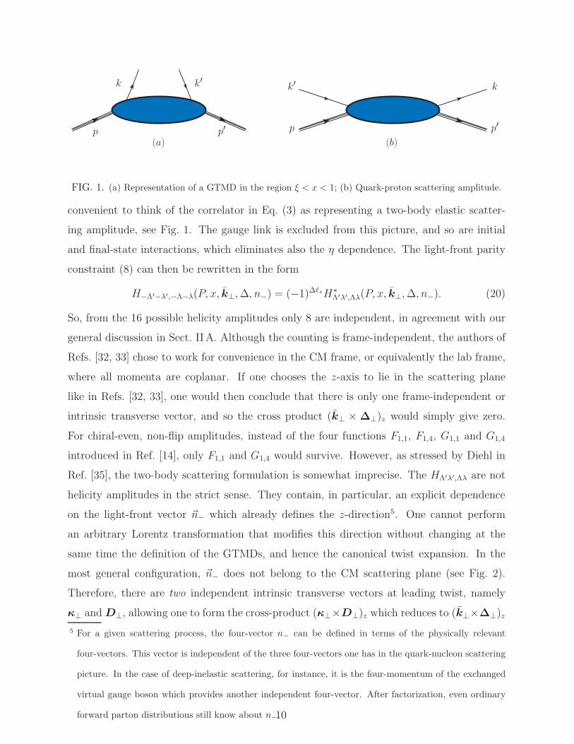
(a) (b)

FIG. 1. (a) Representation of a GTMD in the region ξ < x < 1; (b) Quark-proton scattering amplitude.

convenient to think of the correlator in Eq. (3) as representing a two-body elastic scatter-

ing amplitude, see Fig. 1. The gauge link is excluded from this picture, and so are initial

and final-state interactions, which eliminates also the η dependence. The light-front parity

constraint (8) can then be rewritten in the form

H−Λ′−λ′,−Λ−λ(P, x, k⊥,∆, n−) = (−1)∆ℓzH∗Λ′λ′,Λλ(P, x, k⊥,∆, n−). (20)

So, from the 16 possible helicity amplitudes only 8 are independent, in agreement with our

general discussion in Sect. IIA. Although the counting is frame-independent, the authors of

Refs. [32, 33] chose to work for convenience in the CM frame, or equivalently the lab frame,

where all momenta are coplanar. If one chooses the z-axis to lie in the scattering plane

like in Refs. [32, 33], one would then conclude that there is only one frame-independent or

intrinsic transverse vector, and so the cross product (k⊥ × ∆⊥)z would simply give zero.

For chiral-even, non-flip amplitudes, instead of the four functions F1,1, F1,4, G1,1 and G1,4

introduced in Ref. [14], only F1,1 and G1,4 would survive. However, as stressed by Diehl in

Ref. [35], the two-body scattering formulation is somewhat imprecise. The HΛ′λ′,Λλ are not

helicity amplitudes in the strict sense. They contain, in particular, an explicit dependence

on the light-front vector ~n− which already defines the z-direction5. One cannot perform

an arbitrary Lorentz transformation that modifies this direction without changing at the

same time the definition of the GTMDs, and hence the canonical twist expansion. In the

most general configuration, ~n− does not belong to the CM scattering plane (see Fig. 2).

Therefore, there are two independent intrinsic transverse vectors at leading twist, namely

κ⊥ andD⊥, allowing one to form the cross-product (κ⊥×D⊥)z which reduces to (k⊥×∆⊥)z

5 For a given scattering process, the four-vector n−

can be defined in terms of the physically relevant

four-vectors. This vector is independent of the three four-vectors one has in the quark-nucleon scattering

picture. In the case of deep-inelastic scattering, for instance, it is the four-momentum of the exchanged

virtual gauge boson which provides another independent four-vector. After factorization, even ordinary

forward parton distributions still know about n−.10

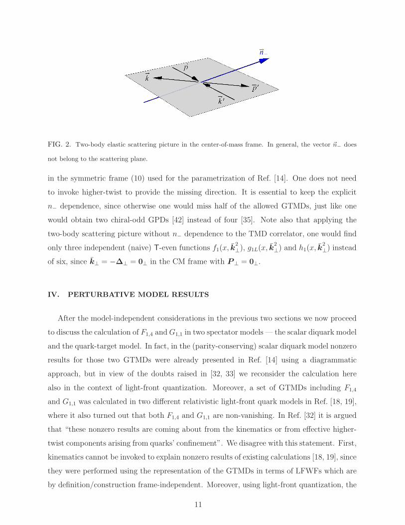
FIG. 2. Two-body elastic scattering picture in the center-of-mass frame. In general, the vector ~n−

does

not belong to the scattering plane.

in the symmetric frame (10) used for the parametrization of Ref. [14]. One does not need

to invoke higher-twist to provide the missing direction. It is essential to keep the explicit

n− dependence, since otherwise one would miss half of the allowed GTMDs, just like one

would obtain two chiral-odd GPDs [42] instead of four [35]. Note also that applying the

two-body scattering picture without n− dependence to the TMD correlator, one would find

only three independent (naive) T-even functions f1(x, k2⊥), g1L(x, k

2⊥) and h1(x, k

2⊥) instead

of six, since k⊥ = −∆⊥ = 0⊥ in the CM frame with P⊥ = 0⊥.

IV. PERTURBATIVE MODEL RESULTS

After the model-independent considerations in the previous two sections we now proceed

to discuss the calculation of F1,4 andG1,1 in two spectator models — the scalar diquark model

and the quark-target model. In fact, in the (parity-conserving) scalar diquark model nonzero

results for those two GTMDs were already presented in Ref. [14] using a diagrammatic

approach, but in view of the doubts raised in [32, 33] we reconsider the calculation here

also in the context of light-front quantization. Moreover, a set of GTMDs including F1,4

and G1,1 was calculated in two different relativistic light-front quark models in Ref. [18, 19],

where it also turned out that both F1,4 and G1,1 are non-vanishing. In Ref. [32] it is argued

that “these nonzero results are coming about from the kinematics or from effective higher-

twist components arising from quarks’ confinement”. We disagree with this statement. First,

kinematics cannot be invoked to explain nonzero results of existing calculations [18, 19], since

they were performed using the representation of the GTMDs in terms of LFWFs which are

by definition/construction frame-independent. Moreover, using light-front quantization, the

11

quark correlation functions (4) entering the calculation of F1,4 and G1,1 have a decomposition

which involve only the “good” light-front components of the fields, and therefore correspond

to pure twist-two contributions (see, for example, Ref. [34]). In this context note also that in

spectator models the active partons are (space-like) off-shell. However, this feature, which is

not specific to the calculation of GTMDs but rather holds even for ordinary forward parton

distributions, does not increase the counting of independent twist-2 functions. Second, as we

discuss in this section, not only the scalar diquark model but also the quark-target model

predicts nonzero results for F1,4 and G1,1. Both models being purely perturbative, this

means that “effective higher twist components arising from quarks’ confinement” cannot be

invoked to explain these results.

That F1,4 and G1,1 are nonzero is a generic feature. They are directly related to the

amount of OAM and spin-orbit correlations inside the target [18, 25–28, 31]. Vanishing F1,4

and G1,1 would therefore imply vanishing (canonical) OAM and spin-orbit correlations. In

order to further solidify the relation between F1,4 and G1,1 and the spin/orbital structure of

the nucleon, we compute the canonical OAM and spin-orbit correlations from the operator

definition in both the scalar diquark model and the quark-target model. They are nonzero

and satisfy the model-independent relations of Refs. [18, 25, 26, 31]

For convenience, we will restrict the discussions in the following to the case ξ = 0.

A. Scalar Diquark Model

We calculate the matrix element in Eq. (3) in the scalar diquark model, i.e., a Yukawa

theory defined by the Lagrangian (see also App. A in Ref. [43])

L = ΨN(i/∂ −M)ΨN + ψ(i/∂ −mq)ψ + (∂µφ ∂µφ∗ −m2

s|φ|2) + gs(ψΨNφ∗ +ΨNψφ), (21)

where ΨN denotes the fermionic target field with mass M , ψ the quark field with mass mq,

and φ the scalar diquark field with mass ms. To leading order in the coupling gs of the

Yukawa interaction, the time-ordered quark correlator reads

〈p′,Λ′|T{ψα(−z2)ψβ(

z2)}|p,Λ〉 = ig2s

∫

d4q

(2π)4[u′(/q −mq −M)]α [(/q −mq −M)u]β

Dq

e−i(P−q)·z

+O(g4s), (22)

where the denominator is Dq = [q2 −m2s + iǫ]

[

(p′ − q)2 −m2q + iǫ

] [

(p− q)2 −m2q + iǫ

]

,

u′ = u(p′,Λ′) and u = u(p,Λ). This expression can be depicted by the diagram on the

12

p p′

p− q p′ − q

q q

p− q p′ − q

p p′

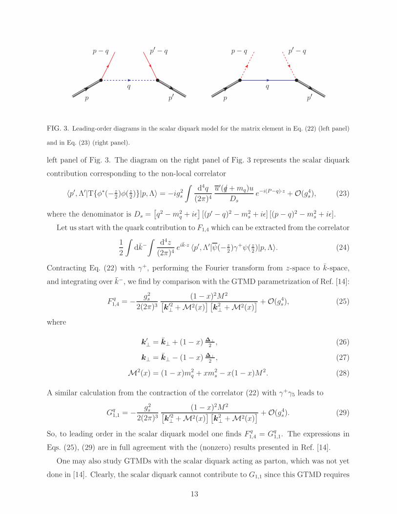
FIG. 3. Leading-order diagrams in the scalar diquark model for the matrix element in Eq. (22) (left panel)

and in Eq. (23) (right panel).

left panel of Fig. 3. The diagram on the right panel of Fig. 3 represents the scalar diquark

contribution corresponding to the non-local correlator

〈p′,Λ′|T{φ∗(−z2)φ( z

2)}|p,Λ〉 = −ig2s

∫

d4q

(2π)4u′(/q +mq)u

Dse−i(P−q)·z +O(g4s), (23)

where the denominator is Ds =[

q2 −m2q + iǫ

]

[(p′ − q)2 −m2s + iǫ] [(p− q)2 −m2

s + iǫ].

Let us start with the quark contribution to F1,4 which can be extracted from the correlator

1

2

∫

dk−∫

d4z

(2π)4eik·z 〈p′,Λ′|ψ(−z

2)γ+ψ( z

2)|p,Λ〉. (24)

Contracting Eq. (22) with γ+, performing the Fourier transform from z-space to k-space,

and integrating over k−, we find by comparison with the GTMD parametrization of Ref. [14]:

F q1,4 = − g2s

2(2π)3(1− x)2M2

[

k′2⊥ +M2(x)

] [

k2⊥ +M2(x)

] +O(g4s), (25)

where

k′⊥ = k⊥ + (1− x) ∆⊥

2, (26)

k⊥ = k⊥ − (1− x) ∆⊥

2, (27)

M2(x) = (1− x)m2q + xm2

s − x(1− x)M2. (28)

A similar calculation from the contraction of the correlator (22) with γ+γ5 leads to

Gq1,1 = − g2s

2(2π)3(1− x)2M2

[

k′2⊥ +M2(x)

] [

k2⊥ +M2(x)

] +O(g4s). (29)

So, to leading order in the scalar diquark model one finds F q1,4 = Gq

1,1. The expressions in

Eqs. (25), (29) are in full agreement with the (nonzero) results presented in Ref. [14].

One may also study GTMDs with the scalar diquark acting as parton, which was not yet

done in [14]. Clearly, the scalar diquark cannot contribute to G1,1 since this GTMD requires

13

p p′

p− q p′ − q

q

q

p− q p′ − q

p p′

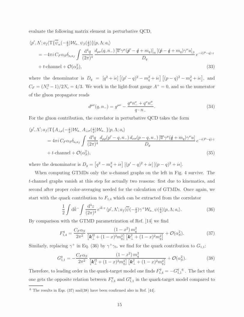
FIG. 4. Leading-order diagrams in the quark-target model (in light-front gauge) for the matrix element

in Eq. (33) (upper row) and in Eq. (35) (lower row). Note that for the amplitude in (35) we only consider

diagrams which eventually could contribute to gluon GTMDs for x ∈ [0, 1].

the active parton to be polarized. The scalar diquark contribution to F1,4 can be extracted

from the correlator

1

2

∫

dk−∫

d4z

(2π)4eik·z 〈p′,Λ′|φ∗(−z

2)i

↔∂+φ( z

2)|p,Λ〉, (30)

where φ∗(−z2)i

↔∂+φ( z

2) = φ∗(−z

2)[i∂+φ( z

2)]−[i∂+φ(−z

2)]φ( z

2) = 2i∂+z [φ

∗(−z2)φ( z

2)]. As a result,

we obtain

F s1,4 = − g2s

2(2π)3x(1− x)M2

[

k′2⊥ +M2(1− x)

] [

k2⊥ +M2(1− x)

] +O(g4s), (31)

Gs1,1 = 0. (32)

B. Quark-Target Model

We continue with the same strategy as above and calculate the GTMDs in QCD for

a quark target |p,Λ; ai〉, where ai(f) is the color of the initial (final) quark. Then, a first

non-trivial perturbative expression for the GTMDs can be extracted from the diagrams in

Fig. 4. We point out that, to the order in perturbation theory considered here, virtual

radiative corrections do not contribute to F1,4 and G1,1. For the quark contribution, we

14

evaluate the following matrix element in perturbative QCD,

〈p′,Λ′; af |T{ψα(−z2)Wn−

ψβ(z2)}|p,Λ; ai〉

= −4πiCFαSδaiaf

∫

d4q

(2π)4dµν(q, n−) [u

′γµ(/p′ − /q +mq)]α [(/p− /q +mq)γνu]β

Dqe−i(P−q)·z

+ t-channel +O(α2S), (33)

where the denominator is Dq = [q2 + iǫ][

(p′ − q)2 −m2q + iǫ

] [

(p− q)2 −m2q + iǫ

]

, and

CF = (N2c − 1)/2Nc = 4/3. We work in the light-front gauge A+ = 0, and so the numerator

of the gluon propagator reads

dµν(q, n−) = gµν − qµnν− + qνnµ

−q · n−

. (34)

For the gluon contribution, the correlator in perturbative QCD takes the form

〈p′,Λ′; af |T{A⊥ρ(−z2)Wn−

A⊥σ(z2)Wn−

}|p,Λ; ai〉

= 4πiCFαSδaiaf

∫

d4q

(2π)4dµρ(p

′ − q, n−) dνσ(p− q, n−) [u′γµ(/q +mq)γ

νu]

Dg

e−i(P−q)·z

+ t-channel +O(α2S), (35)

where the denominator is Dg =[

q2 −m2q + iǫ

]

[(p′ − q)2 + iǫ] [(p− q)2 + iǫ].

When computing GTMDs only the u-channel graphs on the left in Fig. 4 survive. The

t-channel graphs vanish at this step for actually two reasons: first due to kinematics, and

second after proper color-averaging needed for the calculation of GTMDs. Once again, we

start with the quark contribution to F1,4 which can be extracted from the correlator

1

2

∫

dk−∫

d4z

(2π)4eik·z 〈p′,Λ′; af |ψ(−z

2)γ+Wn−

ψ( z2)|p,Λ; ai〉. (36)

By comparison with the GTMD parametrization of Ref. [14] we find

F q1,4 =

CFαS

2π2

(1− x2)m2q

[

k′2⊥ + (1− x)2m2

q

] [

k2⊥ + (1− x)2m2

q

] +O(α2S). (37)

Similarly, replacing γ+ in Eq. (36) by γ+γ5, we find for the quark contribution to G1,1:

Gq1,1 = −CFαS

2π2

(1− x2)m2q

[

k′2⊥ + (1− x)2m2

q

] [

k2⊥ + (1− x)2m2

q

] +O(α2S). (38)

Therefore, to leading order in the quark-target model one finds F q1,4 = −Gq

1,16 . The fact that

one gets the opposite relation between F q1,4 and G

q1,1 in the quark-target model compared to

6 The results in Eqs. (37) and(38) have been confirmed also in Ref. [44].

15

the scalar diquark model is easy to understand from a mathematical point of view. In the

quark-target model there is an extra Dirac matrix to anticommute with γ5 compared to the

scalar diquark model, leading to an extra minus sign in the relation between F q1,4 and Gq

1,1.

Now, the gluon contribution to F1,4 can be extracted from the correlator∫

dk−∫

d4z

(2π)4eik·z 〈p′,Λ′; af | − 2gρσ⊥ Tr[A⊥ρ(−z

2)Wn−

A⊥σ(z2)Wn−

]|p,Λ; ai〉. (39)

As a result, we obtain for x ∈ [0, 1]

F g1,4 =

CFαS

2π2

(1− x)(2− x)m2q

[

k′2⊥ + x2m2

q

] [

k2⊥ + x2m2

q

] +O(α2S). (40)

Similarly, the gluon contribution to G1,1 can be extracted from the correlator∫

dk−∫

d4z

(2π)4eik·z 〈p′,Λ′; af | − 2iǫρσ⊥ Tr[A⊥ρ(−z

2)Wn−

A⊥σ(z2)Wn−

]|p,Λ; ai〉, (41)

where ǫρσ⊥ = ǫρσn+n− with ǫ0123 = +1. This leads us to

Gg1,1 = −CFαS

2π2

1− x

x

[(1− x)2 + 1]m2q

[

k′2⊥ + x2m2

q

] [

k2⊥ + x2m2

q

] +O(α2S). (42)

Obviously, in the quark-target model F1,4 and G1,1 are nonzero for both quarks and

gluons. We performed the calculation of those objects also in Feynman gauge and found the

same results. Note that in Feynman gauge, in the case of quark GTMDs, one also needs

to take into account contributions due to the gauge link of the GTMD correlator (see also

Ref. [43]). While in general those terms matter for GTMDs, the explicit calculation shows

that they do not contribute to F1,4 and G1,1 through O(αS), if one works with either future-

pointing or past-pointing Wilson lines as we do. This also demonstrates, in the context of a

model calculation, that the real part of those two GTMDs does not depend on the direction

of the gauge contour.

C. Canonical Orbital Angular Momentum and Spin-Orbit Correlation

Following the same diagrammatic approach, we now calculate the canonical OAM. The

corresponding operators for quarks, scalar diquarks and gluons with momentum fraction

x ∈ [0, 1] are given in the light-front gauge by

Oqℓz(x, r−, r⊥) ≡

1

2

∫

dz−

2πeixP

+z−[

ψ(r− − z−

2, r⊥) γ

+(r⊥ × i∂⊥)z ψ(r− + z−

2, r⊥)

]

+ h.c.,

(43)

16

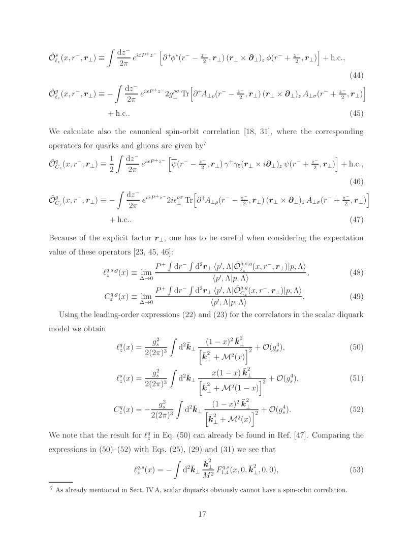
Osℓz(x, r

−, r⊥) ≡∫

dz−

2πeixP

+z−[

∂+φ∗(r− − z−

2, r⊥) (r⊥ × ∂⊥)z φ(r

− + z−

2, r⊥)

]

+ h.c.,

(44)

Ogℓz(x, r−, r⊥) ≡ −

∫

dz−

2πeixP

+z−2gρσ⊥ Tr[

∂+A⊥ρ(r− − z−

2, r⊥) (r⊥ × ∂⊥)z A⊥σ(r

− + z−

2, r⊥)

]

+ h.c.. (45)

We calculate also the canonical spin-orbit correlation [18, 31], where the corresponding

operators for quarks and gluons are given by7

OqCz(x, r−, r⊥) ≡

1

2

∫

dz−

2πeixP

+z−[

ψ(r− − z−

2, r⊥) γ

+γ5(r⊥ × i∂⊥)z ψ(r− + z−

2, r⊥)

]

+ h.c.,

(46)

OgCz(x, r−, r⊥) ≡ −

∫

dz−

2πeixP

+z−2iǫρσ⊥ Tr[

∂+A⊥ρ(r− − z−

2, r⊥) (r⊥ × ∂⊥)z A⊥σ(r

− + z−

2, r⊥)

]

+ h.c.. (47)

Because of the explicit factor r⊥, one has to be careful when considering the expectation

value of these operators [23, 45, 46]:

ℓq,s,gz (x) ≡ lim∆→0

P+∫

dr−∫

d2r⊥ 〈p′,Λ|Oq,s,gℓz

(x, r−, r⊥)|p,Λ〉〈p′,Λ|p,Λ〉 , (48)

Cq,gz (x) ≡ lim

∆→0

P+∫

dr−∫

d2r⊥ 〈p′,Λ|Oq,gCz(x, r−, r⊥)|p,Λ〉

〈p′,Λ|p,Λ〉 . (49)

Using the leading-order expressions (22) and (23) for the correlators in the scalar diquark

model we obtain

ℓqz(x) =g2s

2(2π)3

∫

d2k⊥

(1− x)2 k2⊥

[

k2⊥ +M2(x)

]2 +O(g4s), (50)

ℓsz(x) =g2s

2(2π)3

∫

d2k⊥

x(1 − x) k2⊥

[

k2⊥ +M2(1− x)

]2 +O(g4s), (51)

Cqz (x) = − g2s

2(2π)3

∫

d2k⊥

(1− x)2 k2⊥

[

k2⊥ +M2(x)

]2 +O(g4s). (52)

We note that the result for ℓqz in Eq. (50) can already be found in Ref. [47]. Comparing the

expressions in (50)–(52) with Eqs. (25), (29) and (31) we see that

ℓq,sz (x) = −∫

d2k⊥

k2⊥

M2F q,s1,4 (x, 0, k

2⊥, 0, 0), (53)

7 As already mentioned in Sect. IVA, scalar diquarks obviously cannot have a spin-orbit correlation.

17

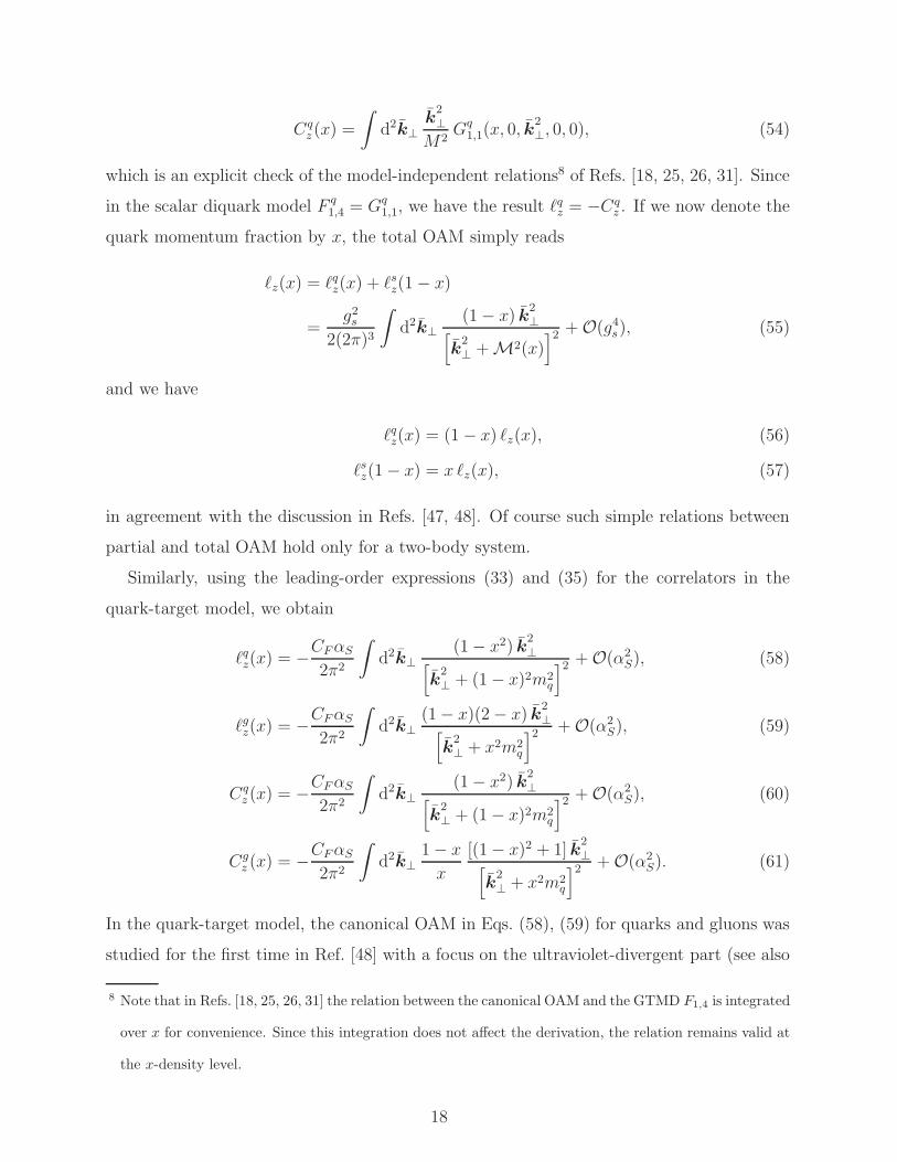
Cqz (x) =

∫

d2k⊥

k2⊥

M2Gq

1,1(x, 0, k2⊥, 0, 0), (54)

which is an explicit check of the model-independent relations8 of Refs. [18, 25, 26, 31]. Since

in the scalar diquark model F q1,4 = Gq

1,1, we have the result ℓqz = −Cqz . If we now denote the

quark momentum fraction by x, the total OAM simply reads

ℓz(x) = ℓqz(x) + ℓsz(1− x)

=g2s

2(2π)3

∫

d2k⊥

(1− x) k2⊥

[

k2⊥ +M2(x)

]2 +O(g4s), (55)

and we have

ℓqz(x) = (1− x) ℓz(x), (56)

ℓsz(1− x) = x ℓz(x), (57)

in agreement with the discussion in Refs. [47, 48]. Of course such simple relations between

partial and total OAM hold only for a two-body system.

Similarly, using the leading-order expressions (33) and (35) for the correlators in the

quark-target model, we obtain

ℓqz(x) = −CFαS

2π2

∫

d2k⊥

(1− x2) k2⊥

[

k2⊥ + (1− x)2m2

q

]2 +O(α2S), (58)

ℓgz(x) = −CFαS

2π2

∫

d2k⊥

(1− x)(2− x) k2⊥

[

k2⊥ + x2m2

q

]2 +O(α2S), (59)

Cqz (x) = −CFαS

2π2

∫

d2k⊥

(1− x2) k2⊥

[

k2⊥ + (1− x)2m2

q

]2 +O(α2S), (60)

Cgz (x) = −CFαS

2π2

∫

d2k⊥

1− x

x

[(1− x)2 + 1] k2⊥

[

k2⊥ + x2m2

q

]2 +O(α2S). (61)

In the quark-target model, the canonical OAM in Eqs. (58), (59) for quarks and gluons was

studied for the first time in Ref. [48] with a focus on the ultraviolet-divergent part (see also

8 Note that in Refs. [18, 25, 26, 31] the relation between the canonical OAM and the GTMD F1,4 is integrated

over x for convenience. Since this integration does not affect the derivation, the relation remains valid at

the x-density level.

18

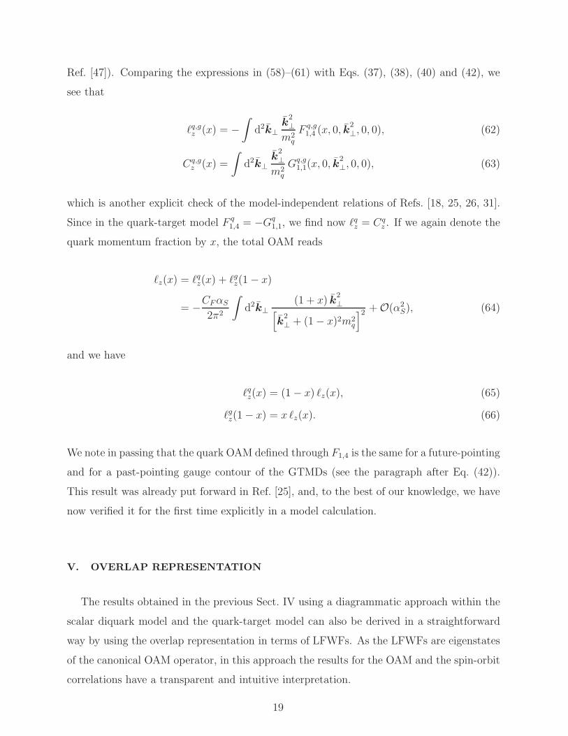
Ref. [47]). Comparing the expressions in (58)–(61) with Eqs. (37), (38), (40) and (42), we

see that

ℓq,gz (x) = −∫

d2k⊥

k2⊥

m2q

F q,g1,4 (x, 0, k

2⊥, 0, 0), (62)

Cq,gz (x) =

∫

d2k⊥

k2⊥

m2q

Gq,g1,1(x, 0, k

2⊥, 0, 0), (63)

which is another explicit check of the model-independent relations of Refs. [18, 25, 26, 31].

Since in the quark-target model F q1,4 = −Gq

1,1, we find now ℓqz = Cqz . If we again denote the

quark momentum fraction by x, the total OAM reads

ℓz(x) = ℓqz(x) + ℓgz(1− x)

= −CFαS

2π2

∫

d2k⊥

(1 + x) k2⊥

[

k2⊥ + (1− x)2m2

q

]2 +O(α2S), (64)

and we have

ℓqz(x) = (1− x) ℓz(x), (65)

ℓgz(1− x) = x ℓz(x). (66)

We note in passing that the quark OAM defined through F1,4 is the same for a future-pointing

and for a past-pointing gauge contour of the GTMDs (see the paragraph after Eq. (42)).

This result was already put forward in Ref. [25], and, to the best of our knowledge, we have

now verified it for the first time explicitly in a model calculation.

V. OVERLAP REPRESENTATION

The results obtained in the previous Sect. IV using a diagrammatic approach within the

scalar diquark model and the quark-target model can also be derived in a straightforward

way by using the overlap representation in terms of LFWFs. As the LFWFs are eigenstates

of the canonical OAM operator, in this approach the results for the OAM and the spin-orbit

correlations have a transparent and intuitive interpretation.

19

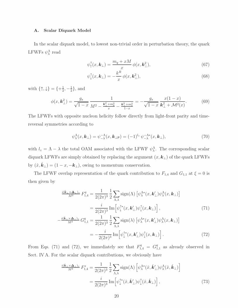
A. Scalar Diquark Model

In the scalar diquark model, to lowest non-trivial order in perturbation theory, the quark

LFWFs ψΛλ read

ψ↑↑(x,k⊥) =

mq + xM

xφ(x,k2

⊥), (67)

ψ↑↓(x,k⊥) = −k

R

xφ(x,k2

⊥), (68)

with {↑, ↓} = {+12,−1

2}, and

φ(x,k2⊥) =

gs√1− x

1

M2 − k2⊥+m2

q

x− k

2⊥+m2

s

1−x

= − gs√1− x

x(1 − x)

k2⊥ +M2(x)

. (69)

The LFWFs with opposite nucleon helicity follow directly from light-front parity and time-

reversal symmetries according to

ψΛλ (x,k⊥) = ψ−Λ

−λ (x,k⊥P) = (−1)lz ψ−Λ∗−λ (x,k⊥), (70)

with lz = Λ − λ the total OAM associated with the LFWF ψΛλ . The corresponding scalar

diquark LFWFs are simply obtained by replacing the argument (x,k⊥) of the quark LFWFs

by (x, k⊥) = (1− x,−k⊥), owing to momentum conservation.

The LFWF overlap representation of the quark contribution to F1,4 and G1,1 at ξ = 0 is

then given by

i(k⊥×∆⊥)zM2 F q

1,4 =1

2(2π)31

2

∑

Λ,λ

sign(Λ)[

ψΛ∗λ (x,k′

⊥)ψΛλ (x,k⊥)

]

=i

2(2π)3Im

[

ψ↑∗↓ (x,k′

⊥)ψ↑↓(x,k⊥)

]

, (71)

− i(k⊥×∆⊥)zM2 Gq

1,1 =1

2(2π)31

2

∑

Λ,λ

sign(λ)[

ψΛ∗λ (x,k′

⊥)ψΛλ (x,k⊥)

]

= − i

2(2π)3Im

[

ψ↑∗↓ (x,k′

⊥)ψ↑↓(x,k⊥)

]

. (72)

From Eqs. (71) and (72), we immediately see that F q1,4 = Gq

1,1 as already observed in

Sect. IVA. For the scalar diquark contributions, we obviously have

i(k⊥×∆⊥)zM2 F s

1,4 =1

2(2π)31

2

∑

Λ,λ

sign(Λ)[

ψΛ∗λ (x, k ′

⊥)ψΛλ (x, k⊥)

]

=i

2(2π)3Im

[

ψ↑∗↓ (x, k ′

⊥)ψ↑↓(x, k⊥)

]

, (73)

20

− i(k⊥×∆⊥)zM2 Gs

1,1 = 0. (74)

Using the explicit expressions (67)-(68) for the quark LFWFs in the scalar diquark model,

we reproduce the results of Sect. IVA.

Since the “parton” OAM is simply given by (1− x) times the total OAM in a two-body

system [47, 48], we can easily write down the overlap representation of the canonical OAM

and spin-orbit correlation for the quark,

ℓqz(x) = (1− x)

∫

d2k⊥

2(2π)31

2

∑

Λ,λ

sign(Λ) lz |ψΛλ (x, k⊥)|2

= (1− x)

∫

d2k⊥2(2π)3

|ψ↑↓(x, k⊥)|2, (75)

Cqz (x) = (1− x)

∫

d2k⊥

2(2π)31

2

∑

Λ,λ

sign(λ) lz |ψΛλ (x, k⊥)|2

= −(1− x)

∫

d2k⊥2(2π)3

|ψ↑↓(x, k⊥)|2, (76)

and the scalar diquark,

ℓsz(x) = (1− x)

∫

d2ˆk⊥2(2π)3

1

2

∑

Λ,λ

sign(Λ) lz |ψΛλ (x,

ˆk⊥)|2

= (1− x)

∫

d2k⊥2(2π)3

|ψ↑↓(1− x, k⊥)|2, (77)

Csz(x) = 0. (78)

The relation ℓqz = −Cqz can now be readily understood in physical terms. In the scalar

diquark model, the total OAM associated with a LFWF lz = Λ− λ is necessarily correlated

with the nucleon helicity Λ and anti-correlated with the quark helicity λ by angular momen-

tum conservation. The “parton” OAM being simply (1− x) times the total OAM, we have

automatically ℓqz = −Cqz > 0 and ℓsz > 0. Finally, we have

Im[

ψ↑∗↓ (x,k′

⊥)ψ↑↓(x,k⊥)

]

= −(1− x)(k⊥ ×∆⊥)z

k2⊥

|ψ↑↓(x, k⊥)|2 +O(∆2

⊥), (79)

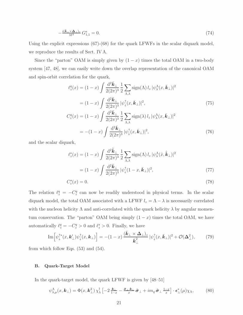
from which follow Eqs. (53) and (54).

B. Quark-Target Model

In the quark-target model, the quark LFWF is given by [48–51]

ψΛλ,µ(x,k⊥) = Φ(x,k2

⊥)χ†λ

[

−2 k⊥

1−x− σ⊥·k⊥

xσ⊥ + imq σ⊥

1−xx

]

· ǫ∗⊥(µ)χΛ, (80)

21

where σ1 = σ2 and σ2 = −σ1, the polarization vectors are defined as ǫ⊥(µ = +1) = − 1√2(1, i)

and ǫ⊥(µ = −1) = 1√2(1,−i), and

Φ(x,k2⊥) =

gT√1− x

x(1− x)

k2⊥ + (1− x)2m2

q

, (81)

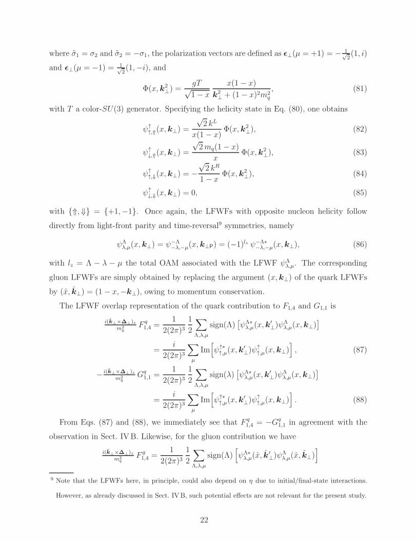
with T a color-SU(3) generator. Specifying the helicity state in Eq. (80), one obtains

ψ↑↑,⇑(x,k⊥) =

√2 kL

x(1 − x)Φ(x,k2

⊥), (82)

ψ↑↓,⇑(x,k⊥) =

√2mq(1− x)

xΦ(x,k2

⊥), (83)

ψ↑↑,⇓(x,k⊥) = −

√2 kR

1− xΦ(x,k2

⊥), (84)

ψ↑↓,⇓(x,k⊥) = 0, (85)

with {⇑,⇓} = {+1,−1}. Once again, the LFWFs with opposite nucleon helicity follow

directly from light-front parity and time-reversal9 symmetries, namely

ψΛλ,µ(x,k⊥) = ψ−Λ

−λ,−µ(x,k⊥P) = (−1)lz ψ−Λ∗−λ,−µ(x,k⊥), (86)

with lz = Λ − λ − µ the total OAM associated with the LFWF ψΛλ,µ. The corresponding

gluon LFWFs are simply obtained by replacing the argument (x,k⊥) of the quark LFWFs

by (x, k⊥) = (1− x,−k⊥), owing to momentum conservation.

The LFWF overlap representation of the quark contribution to F1,4 and G1,1 is

i(k⊥×∆⊥)zm2

qF q1,4 =

1

2(2π)31

2

∑

Λ,λ,µ

sign(Λ)[

ψΛ∗λ,µ(x,k

′⊥)ψ

Λλ,µ(x,k⊥)

]

=i

2(2π)3

∑

µ

Im[

ψ↑∗↑,µ(x,k

′⊥)ψ

↑↑,µ(x,k⊥)

]

, (87)

− i(k⊥×∆⊥)zm2

qGq

1,1 =1

2(2π)31

2

∑

Λ,λ,µ

sign(λ)[

ψΛ∗λ,µ(x,k

′⊥)ψ

Λλ,µ(x,k⊥)

]

=i

2(2π)3

∑

µ

Im[

ψ↑∗↑,µ(x,k

′⊥)ψ

↑↑,µ(x,k⊥)

]

. (88)

From Eqs. (87) and (88), we immediately see that F q1,4 = −Gq

1,1 in agreement with the

observation in Sect. IVB. Likewise, for the gluon contribution we have

i(k⊥×∆⊥)zm2

qF g1,4 =

1

2(2π)31

2

∑

Λ,λ,µ

sign(Λ)[

ψΛ∗λ,µ(x, k

′⊥)ψ

Λλ,µ(x, k⊥)

]

9 Note that the LFWFs here, in principle, could also depend on η due to initial/final-state interactions.

However, as already discussed in Sect. IVB, such potential effects are not relevant for the present study.

22

=i

2(2π)3

∑

µ

Im[

ψ↑∗↑,µ(x, k

′⊥)ψ

↑↑,µ(x, k⊥)

]

, (89)

− i(k⊥×∆⊥)zm2

qGg

1,1 =1

2(2π)31

2

∑

Λ,λ,µ

sign(µ)[

ψΛ∗λ,µ(x, k

′⊥)ψ

Λλ,µ(x, k⊥)

]

=i

2(2π)3

∑

µ

sign(µ) Im[

ψ↑∗↑,µ(x, k

′⊥)ψ

↑↑,µ(x, k⊥)

]

. (90)

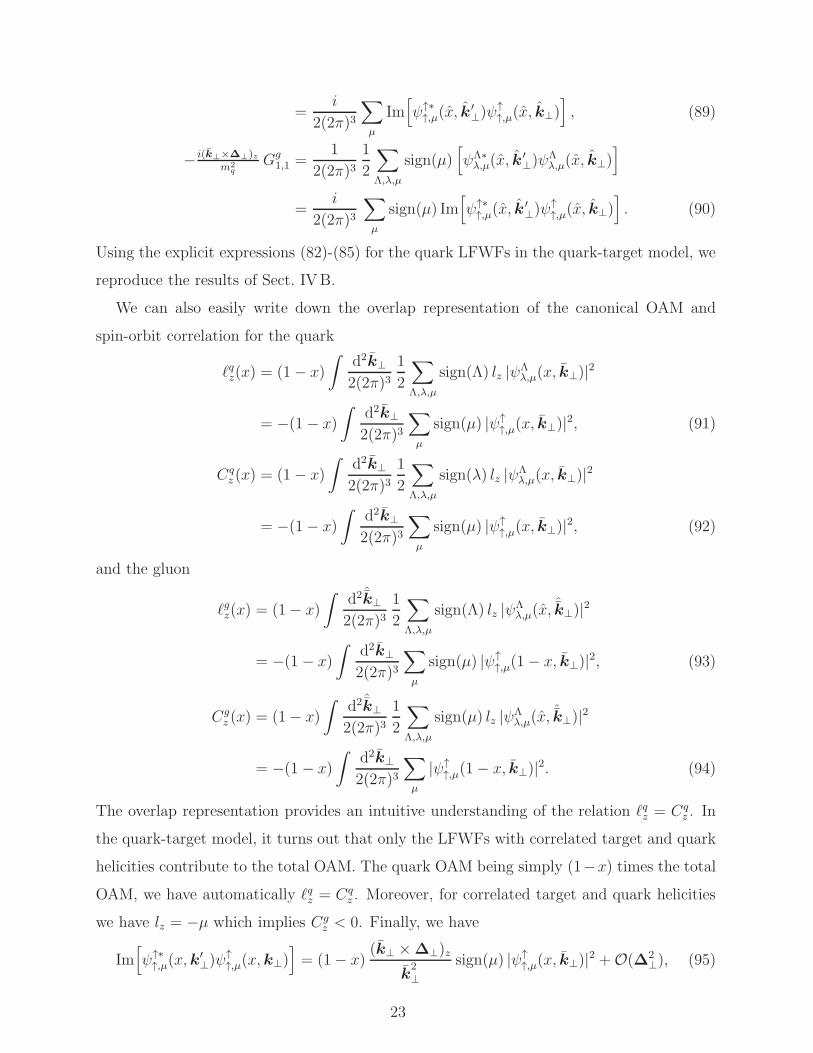
Using the explicit expressions (82)-(85) for the quark LFWFs in the quark-target model, we

reproduce the results of Sect. IVB.

We can also easily write down the overlap representation of the canonical OAM and

spin-orbit correlation for the quark

ℓqz(x) = (1− x)

∫

d2k⊥2(2π)3

1

2

∑

Λ,λ,µ

sign(Λ) lz |ψΛλ,µ(x, k⊥)|2

= −(1 − x)

∫

d2k⊥2(2π)3

∑

µ

sign(µ) |ψ↑↑,µ(x, k⊥)|2, (91)

Cqz (x) = (1− x)

∫

d2k⊥2(2π)3

1

2

∑

Λ,λ,µ

sign(λ) lz |ψΛλ,µ(x, k⊥)|2

= −(1 − x)

∫

d2k⊥2(2π)3

∑

µ

sign(µ) |ψ↑↑,µ(x, k⊥)|2, (92)

and the gluon

ℓgz(x) = (1− x)

∫

d2ˆk⊥2(2π)3

1

2

∑

Λ,λ,µ

sign(Λ) lz |ψΛλ,µ(x,

ˆk⊥)|2

= −(1 − x)

∫

d2k⊥2(2π)3

∑

µ

sign(µ) |ψ↑↑,µ(1− x, k⊥)|2, (93)

Cgz (x) = (1− x)

∫

d2ˆk⊥2(2π)3

1

2

∑

Λ,λ,µ

sign(µ) lz |ψΛλ,µ(x,

ˆk⊥)|2

= −(1 − x)

∫

d2k⊥2(2π)3

∑

µ

|ψ↑↑,µ(1− x, k⊥)|2. (94)

The overlap representation provides an intuitive understanding of the relation ℓqz = Cqz . In

the quark-target model, it turns out that only the LFWFs with correlated target and quark

helicities contribute to the total OAM. The quark OAM being simply (1−x) times the total

OAM, we have automatically ℓqz = Cqz . Moreover, for correlated target and quark helicities

we have lz = −µ which implies Cgz < 0. Finally, we have

Im[

ψ↑∗↑,µ(x,k

′⊥)ψ

↑↑,µ(x,k⊥)

]

= (1− x)(k⊥ ×∆⊥)z

k2⊥

sign(µ) |ψ↑↑,µ(x, k⊥)|2 +O(∆2

⊥), (95)

23

p p′

k k′

= +GTMDs GPDs GPDs

p′p

k′k k′k

p p′

k⊥ ≫ ΛQCD

FIG. 5. Diagrams determining the leading order of quark GTMDs at large transverse momenta.

from which follow Eqs. (62) and (63).

VI. PERTURBATIVE TAIL OF THE GTMDS

In this section we present results for F1,4 and G1,1 at large transverse parton momenta,

where they can be computed in perturbative QCD. For simplicity we restrict the analysis

to the real part of the GTMDs. Details of a corresponding calculation of the large-k⊥

behavior of TMDs can be found in Ref. [52]. Here we generalize these calculations to nonzero

momentum transfer to the nucleon. Like in Sect. IVB, we have used both the light-front

gauge A+ = 0 and the Feynman gauge and have obtained the same results.

While for the quark we consider the correlator in Eq. (2), for the gluon we have

W µν;ρσΛ′Λ (P, k,∆, n−) =

1

k+

∫

d4z

(2π)4eik·z 〈p′,Λ′|T{2Tr[Gµν(−z

2)Wn−

Gρσ( z2)Wn−

]}|p,Λ〉.

(96)

For the calculation of F1,4 and G1,1 through O(αS) the light-like Wilson lines in those

correlators do not give rise to the infamous light-cone singularities. In fact, we have also

performed a study with Wilson lines that are slightly off the light-cone, and in the end one

can take the light-like limit without encountering a divergence. This no longer necessarily

holds for other GTMDs at large transverse momenta.

In the light-front gauge, the large-k⊥ behavior of the quark GTMDs is described pertur-

batively by the two diagrams on the right of Fig. 5. Expressing them by means of Feynman

rules leads to the following formula,

W[Γ]Λ′Λ(P, x, k⊥,∆, n−)

|k⊥|≫ΛQCD

= −i 4παS

∫

d4l

(2π)4

∫

dk−CF I

[Γ]q + TR I

[Γ]g

[

(l − k)2 + iǫ]

[k′2 + iǫ] [k2 + iǫ]+O(α2

s), (97)

24

p p′

k k′

= +GTMDs GPDs GPDs

p′p

k′k k′k

p p′

k⊥ ≫ ΛQCD

FIG. 6. Diagrams determining the leading order of gluon GTMDs at large transverse momenta.

where

I [Γ]q = 14

∑

j

dµν(l − k, n−) Tr[γν/k′Γ/kγµΓj]W

[Γj ]Λ′Λ (P, l,∆, n−), (98)

I [Γ]g = 12Tr

[

/kγσ(/k − /l)γν/k′Γ] 1

l′+ l+W+ν;+σ

Λ′Λ (P, l,∆, n−), (99)

with l′ = l+∆2(k′ = k+∆

2), l = l−∆

2(k = k−∆

2), and the polarization sum dµν from Eq. (34).

We then apply the collinear approximation for the momentum l ≈ [xzP+, 0, 0⊥] in the hard

scattering part, which can be done if we assume that the average proton momentum P has

a large plus-component P+. Accordingly, we take into account only the leading chiral-even

traces with Γj = {γ+, γ+γ5} and Γj = {γ−,−γ−γ5} in the Fierz transformation. We skip

the details of the calculation, which are similar to the ones in Ref. [52], and directly give the

results for the large-k⊥ behavior of F q1,4 and Gq

1,1 at ξ = 0,

F q1,4 =

αS

2π2

∫ 1

x

dz

z

M2[

CF Hq(x

z, 0,−∆2

⊥)− TR (1− z)2 Hg(xz, 0,−∆2

⊥)]

[

k′2⊥ + z(1 − z)

∆2⊥

4

] [

k2⊥ + z(1− z)

∆2⊥

4

] , (100)

Gq1,1 = − αS

2π2

∫ 1

x

dz

z

M2[

CF Hq(x

z, 0,−∆2

⊥) + TR (1− z)2Hg(xz, 0,−∆2

⊥)]

[

k′2⊥ + z(1− z)

∆2⊥

4

] [

k2⊥ + z(1 − z)

∆2⊥

4

]

−∫ 1

x

dz

z

∆2⊥

4TR z(1− z) (2Hg

T + EgT )(

xz, 0,−∆2

⊥)[

k′2⊥ + z(1− z)

∆2⊥

4

] [

k2⊥ + z(1 − z)

∆2⊥

4

]

, (101)

with TR = 12. Here we follow the GPD conventions of Ref. [5].

Similarly, the large-k⊥ behavior of the gluon GTMDs is described perturbatively by the

two diagrams on the right of Fig. 6. Expressing them by means of Feynman rules leads to

the following formula,

1

l′+ l+W+ν;+σ

Λ′Λ (P, x, k⊥,∆, n−)

25

|k⊥|≫ΛQCD

= −i 4παS

∫

d4l

(2π)4

∫

dk−CF I

νσq + CA I

νσg

[

(l − k)2 + iǫ]

[k′2 + iǫ] [k2 + iǫ]+O(α2

s), (102)

where

Iνσq = 12

∑

j

dνν′

(k′, n−) dσσ′

(k, n−) Tr[

γν′(/k − /l)γσ′Γj

]

W[Γj ]Λ′Λ (P, l,∆, n−), (103)

Iνσg = dνν′

(k′, n−) dσ′σ(k, n−) d

ττ ′(l − k, n−) V1,σ′τβ V2,ν′τ ′α1

l′+ l+W+α;+β

Λ′Λ (P, l,∆, n−), (104)

with

V1,σ′τβ = gσ′τ (l − 2k)β + gτβ(k − 2l)σ′ + gβσ′(l + k)τ , (105)

V2,ν′τ ′α = gτ ′ν′(l′ − 2k′)α + gατ ′(k

′ − 2l′)ν′ + gν′α(l′ + k′)τ ′ . (106)

We then find for the large-k⊥ behavior of F g1,4 and Gg

1,1 at ξ = 0 and for x ≥ 0,

F g1,4 =

αS

2π2

∫ 1

x

dz

z

M2[

CF (1− z) Hq(xz, 0,−∆2

⊥) + CA (z2 − 4z + 72) Hg(x

z, 0,−∆2

⊥)]

[

k′2⊥ + z(1 − z)

∆2⊥

4

] [

k2⊥ + z(1− z)

∆2⊥

4

] ,

(107)

Gg1,1 =

αS

2π2

∫ 1

x

dz

z

M2[

CF(1−z)(z−2)

zHq(x

z, 0,−∆2

⊥) + CA (2z2 − 4z + 72− 2

z)Hg(x

z, 0,−∆2

⊥)]

[

k′2⊥ + z(1 − z)

∆2⊥

4

] [

k2⊥ + z(1 − z)

∆2⊥

4

]

+

∫ 1

x

dz

z

∆2⊥

4CA

2(1− 2z)2 (2Hg

T + EgT )(

xz, 0,−∆2

⊥)[

k′2⊥ + z(1 − z)

∆2⊥

4

] [

k2⊥ + z(1 − z)

∆2⊥

4

]

, (108)

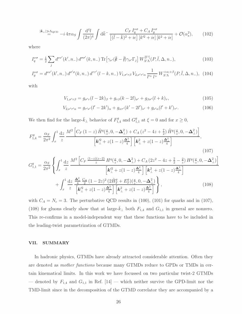
with CA = Nc = 3. The perturbative QCD results in (100), (101) for quarks and in (107),

(108) for gluons clearly show that at large-k⊥ both F1,4 and G1,1 in general are nonzero.

This re-confirms in a model-independent way that these functions have to be included in

the leading-twist parametrization of GTMDs.

VII. SUMMARY

In hadronic physics, GTMDs have already attracted considerable attention. Often they

are denoted as mother functions because many GTMDs reduce to GPDs or TMDs in cer-

tain kinematical limits. In this work we have focussed on two particular twist-2 GTMDs

— denoted by F1,4 and G1,1 in Ref. [14] — which neither survive the GPD-limit nor the

TMD-limit since in the decomposition of the GTMD correlator they are accompanied by a

26

factor that is linear in both the transverse parton momentum and the transverse-momentum

transfer to the nucleon. In some sense this makes these two functions actually unique. The

particular role played by F1,4 and G1,1 is nicely reflected by their intimate connection to

the orbital angular momentum of partons in a longitudinally polarized nucleon and in an

unpolarized nucleon, respectively [18, 25–28, 31]. Those relations open up new opportunities

to study the spin/orbital structure of the nucleon. For instance, new insights in this area

could now be obtained through Lattice QCD, given the related pioneering and encouraging

studies of TMDs and other parton correlation functions in Refs. [53–56].

Our main intention in this paper has been to address recent criticism according to which

even the mere existence of F1,4 and G1,1 is questionable [32, 33]. To this end we have

shown in a model-independent way why the criticism of [32, 33] does not hold. We have

also computed F1,4 and G1,1 in the scalar diquark model of the nucleon, in the quark-target

model, and in perturbative QCD for large transverse parton momenta, and we generally

have found nonzero results in lowest nontrivial order in perturbation theory. Moreover, in

the two spectator models we have verified explicitly the relation between the two GTMDs

and the OAM of partons. In summary, we hope that our work helps to resolve any potential

doubt/confusion with regard to the status of the GTMDs F1,4 and G1,1 and their relation

to the spin/orbital structure of the nucleon.

ACKNOWLEDGMENTS

This work has been supported by the Grant-in-Aid for Scientific Research from the Japan

Society of Promotion of Science under Contract No. 24.6959 (K.K.), the Belgian Fund F.R.S.-

FNRS via the contract of Charge de recherches (C.L.), the National Science Foundation

under Contract No. PHY-1205942 (A.M.), and the European Community Joint Research

Activity “Study of Strongly Interacting Matter” (acronym HadronPhysics3, Grant Agree-

ment No. 283286) under the Seventh Framework Programme of the European Community

(B.P.). The Feynman diagrams in this paper were drawn using JaxoDraw [57].

[1] D. Muller, D. Robaschik, B. Geyer, F. -M. Dittes and J. Horejsi, Fortsch. Phys. 42, 101 (1994).

[2] X.-D. Ji, Phys. Rev. Lett. 78, 610 (1997).

27

[3] A. V. Radyushkin, Phys. Lett. B 380, 417 (1996).

[4] K. Goeke, M. V. Polyakov and M. Vanderhaeghen, Prog. Part. Nucl. Phys. 47, 401 (2001).

[5] M. Diehl, Phys. Rept. 388, 41 (2003).

[6] A. V. Belitsky and A. V. Radyushkin, Phys. Rept. 418, 1 (2005).

[7] S. Boffi and B. Pasquini, Riv. Nuovo Cim. 30, 387 (2007).

[8] A. Bacchetta, M. Diehl, K. Goeke, A. Metz, P. J. Mulders and M. Schlegel, JHEP 0702, 093

(2007).

[9] U. D’Alesio and F. Murgia, Prog. Part. Nucl. Phys. 61, 394 (2008).

[10] M. Burkardt, C. A. Miller and W. D. Nowak, Rept. Prog. Phys. 73, 016201 (2010).

[11] V. Barone, F. Bradamante and A. Martin, Prog. Part. Nucl. Phys. 65, 267 (2010).

[12] C. A. Aidala, S. D. Bass, D. Hasch and G. K. Mallot, Rev. Mod. Phys. 85, 655 (2013).

[13] S. Meissner, A. Metz, M. Schlegel and K. Goeke, JHEP 0808, 038 (2008).

[14] S. Meissner, A. Metz and M. Schlegel, JHEP 0908, 056 (2009).

[15] C. Lorce and B. Pasquini, JHEP 1309, 138 (2013).

[16] X.-D. Ji, Phys. Rev. Lett. 91, 062001 (2003).

[17] A. V. Belitsky, X.-D. Ji and F. Yuan, Phys. Rev. D 69, 074014 (2004).

[18] C. Lorce and B. Pasquini, Phys. Rev. D 84, 014015 (2011).

[19] C. Lorce, B. Pasquini and M. Vanderhaeghen, JHEP 1105, 041 (2011).

[20] A. D. Martin, M. G. Ryskin and T. Teubner, Phys. Rev. D 62, 014022 (2000).

[21] V. A. Khoze, A. D. Martin and M. G. Ryskin, Eur. Phys. J. C 14, 525 (2000).

[22] A. D. Martin and M. G. Ryskin, Phys. Rev. D 64, 094017 (2001).

[23] E. Leader and C. Lorce, [arXiv:1309.4235 [hep-ph]].

[24] M. Wakamatsu, Int. J. Mod. Phys. A 29, 1430012 (2014).

[25] Y. Hatta, Phys. Lett. B 708, 186 (2012).

[26] C. Lorce, B. Pasquini, X. Xiong and F. Yuan, Phys. Rev. D 85, 114006 (2012).

[27] X. Ji, X. Xiong and F. Yuan, Phys. Rev. Lett. 109, 152005 (2012).

[28] C. Lorce, Phys. Lett. B 719, 185 (2013).

[29] R. L. Jaffe and A. Manohar, Nucl. Phys. B 337, 509 (1990).

[30] M. Burkardt, Phys. Rev. D 88, 014014 (2013).

[31] C. Lorce, arXiv:1401.7784 [hep-ph].

[32] S. Liuti, A. Courtoy, G. R. Goldstein, J. O. G. Hernandez and A. Rajan,

28

Int. J. Mod. Phys. Conf. Ser. 25, 1460009 (2014).

[33] A. Courtoy, G. R. Goldstein, J. O. G. Hernandez, S. Liuti and A. Rajan, Phys. Lett. B 731,

141 (2014).

[34] R. L. Jaffe, In ”Erice 1995, The spin structure of the nucleon”, 42-129 [hep-ph/9602236].

[35] M. Diehl, Eur. Phys. J. C 19, 485 (2001).

[36] D. E. Soper, Phys. Rev. D 5, 1956 (1972).

[37] C. E. Carlson and C. -R. Ji, Phys. Rev. D 67, 116002 (2003).

[38] S. J. Brodsky, S. Gardner and D. S. Hwang, Phys. Rev. D 73, 036007 (2006).

[39] M. E. Peskin and D. V. Schroeder, Reading, USA: Addison-Wesley (1995) 842 p

[40] M. Burkardt, Phys. Rev. D 62, 071503 (2000) [Erratum-ibid. D 66, 119903 (2002)].

[41] M. Burkardt, Int. J. Mod. Phys. A 18, 173 (2003).

[42] P. Hoodbhoy and X. -D. Ji, Phys. Rev. D 58, 054006 (1998).

[43] S. Meissner, A. Metz and K. Goeke, Phys. Rev. D 76, 034002 (2007).

[44] A. Mukherjee, S. Nair and V. K. Ojha, arXiv:1403.6233 [hep-ph].

[45] P. Hagler, A. Mukherjee and A. Schafer, Phys. Lett. B 582, 55 (2004).

[46] B. L. G. Bakker, E. Leader and T. L. Trueman, Phys. Rev. D 70, 114001 (2004).

[47] M. Burkardt and H. BC, Phys. Rev. D 79, 071501 (2009).

[48] A. Harindranath and R. Kundu, Phys. Rev. D 59, 116013 (1999).

[49] S. J. Brodsky, D. S. Hwang, B. -Q. Ma and I. Schmidt, Nucl. Phys. B 593, 311 (2001).

[50] A. Harindranath, A. Mukherjee and R. Ratabole, Phys. Rev. D 63, 045006 (2001).

[51] R. Kundu and A. Metz, Phys. Rev. D 65, 014009 (2001).

[52] A. Bacchetta, D. Boer, M. Diehl and P. J. Mulders, JHEP 0808, 023 (2008).

[53] P. Hagler, B. U. Musch, J. W. Negele and A. Schafer, Europhys. Lett. 88, 61001 (2009).

[54] B. U. Musch, P. Hagler, J. W. Negele and A. Schafer, Phys. Rev. D 83, 094507 (2011).

[55] B. U. Musch, P. Hagler, M. Engelhardt, J. W. Negele and A. Schafer, Phys. Rev. D 85, 094510

(2012).

[56] X.-D. Ji, Phys. Rev. Lett. 110, 262002 (2013).

[57] D. Binosi, J. Collins, C. Kaufhold and L. Theussl, Comput. Phys. Commun. 180, 1709 (2009).

29