Two-agent single-machine scheduling with assignable due dates

Applied Mathematics and Computation 219 (2012) 1674–1685

Contents lists available at SciVerse ScienceDirect

Applied Mathematics and Computation

journal homepage: www.elsevier .com/ locate /amc

Two-agent single-machine scheduling with assignable due dates

Yunqiang Yin a,b, Shuenn-Ren Cheng c, T.C.E. Cheng d, Chin-Chia Wu e, Wen-Hsiang Wu f,⇑a State Key Laboratory Breeding Base of Nuclear Resources and Environment, East China Institute of Technology, Nanchang 330013, Chinab School of Sciences, East China Institute of Technology, Fuzhou, Jiangxi 344000, Chinac Graduate Institute of Business Administration, Cheng Shiu University, Kaohsiung County, Taiwand Department of Logistics and Maritime Studies, The Hong Kong Polytechnic University, Hung Hom, Kowloon, Hong Konge Department of Statistics, Feng Chia University, Taichung, Taiwanf Department of Healthcare Management, Yuanpei University, Hsinchu, Taiwan

a r t i c l e i n f o a b s t r a c t

Keywords:SchedulingSingle machineTwo agentsAssignable due dates

0096-3003/$ - see front matter � 2012 Elsevier Inchttp://dx.doi.org/10.1016/j.amc.2012.08.008

⇑ Corresponding author.E-mail address: [email protected] (

We consider several two-agent scheduling problems with assignable due dates on a singlemachine, where each of the agents wants to minimize a measure depending on the com-pletion times of its own jobs and the due dates are treated as given variables and mustbe assigned to individual jobs. The goal is to assign a due date from a given set of due datesand a position in the sequence to each job so that the weighted sum of the objectives ofboth agents is minimized. For different combinations of the objectives, which includethe maximum lateness, total (weighted) tardiness, and total (weighted) number of tardyjobs, we provide the complexity results and solve the corresponding problems, if possible.

� 2012 Elsevier Inc. All rights reserved.

1. Introduction

Since Baker and Smith [4] and Agnetis et al. [1] first studied the scheduling problem with two agents, scheduling withmultiple agents has attracted increasing attention of the scheduling research community. In this problem there are twoagents that compete on the use of a common processor (machine). Each of the agents has a set of jobs that have to be pro-cessed on the same machine without preemption. Each of the agents wants to minimize an objective function that dependson the completion time of its own jobs. The problem is to find a schedule that performs well with respect to the objectives ofboth agents. Such scheduling problems arise in different application contexts, including real-time systems, integrated servicenetworks, industrial districts, telecommunication systems, and so on.

Yuan et al. [41] find that two dynamic programming recursions proposed in Baker and Smith [4] are incorrect and present apolynomial-time algorithm for the same problems. Ng et al. [25] consider two-agent scheduling on a single machine to min-imize the total completion time of the first agent with the restriction that the number of tardy jobs of the second agent cannotexceed a given number. Cheng et al. [7] consider the feasibility model of multi-agent scheduling on a single machine whereeach agent’s objective is to minimize the total weighted number of tardy jobs. Agnetis et al. [2] analyze the complexity of somemulti-agent scheduling problems on a single machine and propose solution algorithms. Cheng et al. [8] study multi-agentscheduling on a single machine where the objectives of the agents are of the max-form. They prove that the feasibility modelis polynomially solvable even when the jobs are subject to precedence restrictions and that the minimization model is stronglyNP-hard in general. Agnetis et al. [3] develop branch-and-bound algorithms for several NP-hard two-agent schedulingproblems. Lee et al. [17] focus on minimizing the total weighted completion time, and introduce fully polynomial-time approx-imation schemes and an efficient approximation algorithm with a reasonable worst-case error bound. Leung et al. [18] expand

. All rights reserved.

W.-H. Wu).

http://dx.doi.org/10.1016/j.amc.2012.08.008

mailto:[email protected]

http://dx.doi.org/10.1016/j.amc.2012.08.008

http://www.sciencedirect.com/science/journal/00963003

http://www.elsevier.com/locate/amc

Y. Yin et al. / Applied Mathematics and Computation 219 (2012) 1674–1685 1675

the framework for the two-agent scheduling problem by including the total tardiness objective, allowing for preemptions, andconsidering jobs with different release dates. They establish the relationships between two-agent scheduling and other areaswithin the scheduling field, namely rescheduling and scheduling, subject to availability constraints. Cheng et al. [5] consider atwo-agent scheduling problem in which the actual processing time of a job in a schedule is a function of the sum of processingtimes of the jobs already processed. The objective is to minimize the total weighted completion time of the jobs of the firstagent with the restriction that no tardy job is allowed for the second agent. They develop a branch-and-bound and three sim-ulated annealing algorithms to solve the problem. Wan et al. [32] consider several two-agent scheduling problems with con-trollable job processing times, where the agents share either a single machine or two identical machines in parallel. Mor andMosheiov [22] consider scheduling with two competing agents to minimize the minmax and minsum earliness measures. Theyfocus on minimizing the maximum earliness or total (weighted) earliness of one agent, subject to an upper bound on the max-imum earliness of the other agent. Mor and Mosheiov [23] address a two-agent problem in the context of batch scheduling on asingle machine with the objective function of minimizing the flowtime of one agent subject to an upper bound on the flowtimeof the second agent. They introduce an efficient Oðn3

2Þ solution algorithm (where n is the total number of jobs). Yin et al. [39]study a scheduling environment with two agents and linear non-increasing job deterioration. They consider three differentobjective functions for one agent, including the maximum earliness cost, total earliness cost, and total weighted earliness cost,while keeping the maximum earliness cost of the other agent below or at a fixed level U, where U is a given big number. Theyprovide the optimal (nondominated) properties and present the complexity results for the problems. Liu et al. [19,20]addressed several two-agent scheduling problems with time-dependent processing times. More recently, Cheng et al. [9]addressed a two-agent scheduling with position- based deteriorating jobs and learning effects, meanwhile, Yin et al. [40]studied a two-agent single-machine scheduling with release times and deadlines.

On the other hand, scheduling problems with due date assignment have received considerable attention in the last twodecades following the wide adoption of new operations management concepts and methods such as just-in-time productionand supply chain management. In traditional scheduling due dates are considered as externally given. A typical problemfaced by a shop supervisor is to schedule jobs on one or more machines to minimize some objective function related tothe due dates, such as the maximum lateness, total tardiness, or number of tardy jobs. An alternative view is to treat duedates as decision variables and to simultaneously assign them while sequencing the jobs. The problem of assigning due datesis also called due date determination.

Popular methods for due date determination use formulas with adjustable parameters that reflect the characteristics of aparticular job, such as its processing time pi. For example, in the common due date determination (CON) method, all the jobsare given a constant due date so di ¼ d; when using the slack (SLK) due date determination method, each job is given a com-mon waiting time or slack, so di ¼ pi þ d; in the processing-time-plus-wait (PPW) due date determination method, whichcontains SLK as a special case, due dates are given by di ¼ kpi þ d, where k is a nonnegative parameter. For research resultson due date determination, the reader may refer to [6,10–12,14,15,24,27,28,16,21,33,35,34,36–38], and so on.

An alternative concept, referred to as generalized due dates (GDD), was first proposed by Hall [13], and studied by Srisk-andarajah [29], and Tanaka and Vlach [30,31]. In the GDD model, there are n jobs and n given due dates, but each due date isnot associated with a specific job. They are assigned to the jobs sequentially. In other words, the job that is completed first isassigned the earliest due date, the job completed second is assigned the second earliest due date, and so on. This situation ismost appropriate when the jobs are interchangeable so that what matters is how many jobs have been completed at somepoint in time rather than which jobs have been completed. Hall [13] suggested several applications in public utility planning,survey design, and flexible manufacturing. Qi et al. [26] studied a new model that generalizes the GDD model. In their model,a set of n due dates are given, on each of which one of the n jobs is expected to be completed. The job assignments are arbi-trary. They referred to this situation as scheduling with assignable due dates and provided complexity results for a variety ofsingle-machine problems. For an example of an application of scheduling with assignable due dates, consider airline indus-try. Given a published flight schedule and corresponding requirement for crew resources, airlines need to decide when andhow many pilots and flight attendants to hire, train, and deploy. Many pilots, for example, regularly request a change in theirposition (as defined by a home base, an equipment type, and a cockpit seat). When changes are approved training is requiredbefore the move can take place. The related planning problem can be modelled as a machine scheduling problem withassignable due dates. In this interpretation, the processing time corresponds to the training time, which is pilot-dependent,and the machine resources correspond to the training capacity. The number of qualified pilots in a certain position, however,does not depend on who they are; the only consideration is that there is a sufficient number to meet demand. As such, aschedule must be devised that assures that enough pilots are available at a specific time. Inspired by the ideas of Bakerand Smith [4] and Qi et al.[26], we introduce a new scheduling model in which both two agents and assignable due datesexist simultaneously. We combine the two agents’ objectives into a single criterion in the weighted-sum form. The objectiveswe consider in this paper are the maximum lateness, total (weighted) tardiness, and total (weighted) number of tardy jobs.We consider different scenarios with assignable due dates, depending on the objective of each agent, and address the com-plexity and solvability of the corresponding problems. This paper is organized as follows: in Section 2 we formulate the gen-eral model and provide some basic properties. In Section 3 we show that the problems where one agent’s objective is any oneof maximum lateness, total tardiness, and (total weighted) number of tardy jobs, while the other agent’s objective is max-imum lateness can be solved in polynomial time or pseudopolynomial time. In Section 4 we show that when the objectives ofboth agents are total tardiness, the problem can be solved in polynomial time. In Section 5 we show that when one agent’sobjective is total weighted tardiness, while the other agent’s objective is any one of maximum lateness, total (weighted)

1676 Y. Yin et al. / Applied Mathematics and Computation 219 (2012) 1674–1685

tardiness, and total (weighted) number of tardy jobs, the problems are unary NP-hard. In Section 6 we show that when oneagent’s objective is total weighted number of tardy jobs, while the other agent’s objective is total tardiness, the problem isbinary NP-hard. We develop a pseudopolynomial-time dynamic programming algorithm for this problem. We conclude thepaper and suggest some future research topics in the last section.

2. Preliminaries

Suppose that there are two competing agents, called agents A and B, respectively. Each of them has a set of non-preemp-tive jobs to be processed on a common machine. Agent A has to execute the job set JA ¼ fJA

1; JA2; . . . ; JA

nAg, whereas agent B has to

execute the job set JB ¼ fJB1; J

B2; . . . ; JB

nBg. All the jobs have a zero release time. Let X 2 fA;Bg. The jobs of agent X are called X-

jobs. The processing time and weight of job JXj in the set JX are positive integers pX

j and wXj , respectively, for all

j 2 f1;2; . . . ;nXg, where pX1 6 pX

2 6 . . . 6 pXnX

. In addition, we are given a set of nX positive integers dX1 6 dX

2 6 . . . 6 dXnX

corre-

sponding to the due dates of agent X and let P ¼PnA

j¼1pAj þ

PnBj¼1pB

j . Both pXj and dX

j for j 2 f1;2; . . . ;nXg are model parameters.The problem is to assign a due date and a position in the sequence to each job so that the weighted sum of the objectives ofagents A and B is minimized. The following symbols are used to represent the problem variables.

dX½j� = due date assigned to job JX

j in a schedule,

CXj = completion time of job JX

j in a schedule,

LXj ¼ CX

j � dX½j�, lateness of job JX

j in a schedule,

TXj ¼maxfLX

j ;0g, tardiness of job JXj in a schedule,

UXj ¼ 1 if CX

j > dX½j� and UX

j ¼ 0 otherwise,

LXmax ¼maxj¼1;2;...;nXfL

Xj g.

Following Qi et al. [26], with respect to indices, when square brackets are used on due dates, i.e., [j], we refer to the due

date assigned to job JXj ; otherwise we refer to the due date dX

j . By an SPT-EDD schedule, we mean a schedule constructed byassigning due dates in the earliest due date (EDD) order to the jobs scheduled in the shortest processing time (SPT) order. Theobjectives investigated include the maximum lateness, total (weighted) tardiness, and total (weighted) number of tardy jobs.

Following Baker and Smith [4], we consider different combinations of the objectives of agents A and B in our model. Whenobjective cA applies to agent A and objective cB applies to agent B, we take the overall scheduling criterion as cA þ hcB, whereh > 0 is simply a weighting factor that helps to keep the two objectives commensurate. In the sequel, adopting the standardnotation for describing scheduling problems, we refer to the problems considered here as 1jdA

½j�; dB½j� jcA þ hcB, where

cA 2 fLAmax;

PTA

j ;P

wAj TA

j ;P

UAj ;P

wAj UA

j g and cB 2 fLBmax;

PTB

j ;P

wBj TB

j ;P

UBj ;P

wBj UB

j g. Note that all these objectives are reg-ular (i.e., nondecreasing in the completion time). Hence there is no benefit in keeping the machine idle, so we begin process-ing each job as soon as the previous job in the sequence is completed.

We say that a schedule S for 1jdA½j�; d

B½j�jcA þ hcB, where cA 2 fLA

max;P

TAj g and cB 2 fLB

max;P

TBj g, is regular if S sequences the

X-jobs (X 2 fA;Bg) in the SPT-EDD order.We say that a schedule S for 1jdA

½j�; dB½j�jcA þ hcB, where cA 2 fLA

max;P

TAj g and cB ¼

PUB

j , is regular if S sequences the A-jobsin the SPT-EDD order and the B-jobs in the SPT order.

We say that a schedule S for 1jdA½j�; d

B½j� jcA þ hcB, where cA ¼ cB ¼

PUB

j , is regular if S sequences the X-jobs (X 2 fA;Bg) in theSPT order.

Next we provide some basic properties of the structures of an optimal schedule. We state each result from the perspectiveof agent A, but the properties apply symmetrically to agent B as well.

Lemma 2.1. If cA ¼ LAmax, then there exists an optimal schedule in which the A-jobs are scheduled in the SPT-EDD order.

Proof. Consider an optimal schedule S in which the A-jobs are not scheduled in the SPT-EDD order. There are two cases toconsider.

Case 1: The A-jobs in S are not scheduled in the SPT order. Let JAl and JA

h be the first pair of jobs such that pAl > pA

h . In thisschedule, job JA

l is scheduled earlier, then a set of B-jobs are consecutively scheduled (with a total load of, say, p), and thenjob JA

h . Suppose that the starting time of JAl is t. Then CA

l ðSÞ ¼ t þ pAl and CA

hðSÞ ¼ t þ pAl þ PðpÞ þ pA

h , where PðpÞ is the totalprocessing time of job set p. So we have

LAl ðSÞ ¼ t þ pA

l � dA½l�ðSÞ

and

LAhðSÞ ¼ t þ pA

l þ PðpÞ þ pAh � dA

½h�ðSÞ:


We create from S a new schedule S0 by interchanging jobs JAl and JA

h , as well as their due date assignments, and leaving theother jobs unchanged in S. Thus, the completion times of the jobs processed before job JA

l and the jobs processed after job JAh in

S are not affected. Moreover, since pAl > pA

h , the jobs in p are scheduled earlier in S0. Thus the objective value of agent B in S0

will not be greater than that in S since objective cB is regular. On the other hand, in S0;CAhðS

0Þ ¼ t þ pAh ,

CAl ðS

0Þ ¼ t þ pAh þ PðpÞ þ pA

l ; dA½h�ðS

0Þ ¼ dA½l�ðSÞ and dA

½l�ðS0Þ ¼ dA

½h�ðSÞ. So we have

LAl ðS

0Þ ¼ t þ pAh þ PðpÞ þ pA

l � dA½h�ðSÞ ¼ LA

hðSÞ

and

LAhðS

0Þ ¼ t þ pAh � dA

½l�ðSÞ 6 t þ pAl � dA

½l�ðSÞ ¼ LAl ðSÞ:

It follows that the maximum lateness of agent A in S0 cannot be greater than that in S.Case 2: The A-jobs in S are scheduled in the SPT order but the due dates are not assigned in nondecreasing order. Let JA

land JA

h be the first pair of jobs such that dA½l�ðSÞ > dA

½h�ðSÞ. In this schedule, job JAl is scheduled earlier, then a set of B-jobs are

consecutively scheduled (with a total load of, say, p), and then job JAh . Suppose that the starting time of JA

l is t. ThenLA

l ðSÞ ¼ t þ pAl � dA

½l�ðSÞ and LAhðSÞ ¼ t þ pA


½h�ðSÞ. We create from S a new schedule S0 by interchanging the twodue dates and leaving the other due dates unchanged in S. Thus, the completion times of all the jobs in JA [ JB remainunchanged in S0. We have

LAl ðS

0Þ ¼ t þ pAl � dA

½h�ðSÞ 6 t þ pAl þ PðpÞ þ pA

h � dA½h�ðSÞ ¼ LA

hðSÞ

and

LAhðS

0Þ ¼ t þ pAl þ PðpÞ þ pA

h � dA½l�ðSÞ 6 t þ pA


½h�ðSÞ ¼ LAhðSÞ:

It follows that S0 is not a worse schedule than S.Thus, repeating this interchange argument for all the A-jobs not sequenced in the SPT-EDD order yields the result. h

Lemma 2.2. If cA ¼P

TAj , then there exists an optimal schedule in which the A-jobs are scheduled in the SPT-EDD order.

Proof. Consider an optimal schedule S in which the A-jobs are not scheduled in the SPT-EDD order. There are two cases toconsider.

Case 1: The A-jobs in S are not scheduled in the SPT order. Let JAl and JA

h be the first pair of jobs such that pAl > pA

h . In thisschedule, job JA

l is scheduled earlier, then a set of B-jobs are consecutively scheduled, and then job JAh . We create from S a new

schedule S0 by interchanging jobs JAl and JA

h , as well as their due date assignments, and leaving the other jobs unchanged in S.By the proof of Lemma 2.1, we know that the objective value of agent B in S0 will not be greater than that in S, andTA

l ðS0Þ ¼ fLA

l ðS0Þ;0g ¼ fLA

hðSÞ;0g ¼ TAhðSÞ and TA

hðS0Þ ¼ fLA

hðS0Þ;0g 6 fLA

l ðSÞ;0g ¼ TAl ðSÞ, implying that S0 is not a worse schedule

than S.Case 2: The A-jobs in S are scheduled in the SPT order but the due dates are not assigned in nondecreasing order. Let JA

l and JAh

be the first pair of jobs such that dA½l�ðSÞ > dA

½h�ðSÞ. In this schedule, job JAl is scheduled earlier, then a set of B-jobs are consecutively

scheduled (with a total load of, say, p), and then job JAh . We create from S a new schedule S0 by interchanging the two due dates,

and leaving the other due dates unchanged in S. Thus, the completion times of all the jobs in JA [ JB remain unchanged in S0, and

analogues to the proof of Lemma 2.1, we have TAl ðSÞ ¼maxft þ pA

l � dA½l�ðSÞ;0g; TA

hðSÞ ¼maxft þ pAl þ PðpÞ þ pA

h � dA½h�ðSÞ; 0g;

TAl ðS0Þ ¼maxft þ pA

l � dA½h�ðSÞ;0g and TA

hðS0Þ ¼maxft þ pA


½l�ðSÞ;0g. In what follows we prove that S0 is not a

worse schedule than S and it suffices to show that TAhðS0Þ þ TA

l ðS0Þ 6 TA

l ðSÞ þ TAhðSÞ. We consider the following cases.

Case 1: t þ pAl 6 dA

½h�ðSÞ and t þ pAl þ PðpÞ þ pA

h 6 dA½l�ðSÞ. Then

TAl ðSÞ þ TA

hðSÞ � ðTAhðS

0Þ þ TAl ðS

0ÞÞ ¼ TAl ðSÞ þ TA

hðSÞ � ð0þ 0Þ ¼ TAl ðSÞ þ TA

hðSÞP 0:

Case 2: dA½h�ðSÞ < t þ pA

l and t þ pAl þ PðpÞ þ pA

h 6 dA½l�ðSÞ. Then

TAl ðSÞ þ TA

hðSÞ � ðTAhðS

0Þ þ TAl ðS

0ÞÞ ¼ TAl ðSÞ þ ðt þ pA


½h�ðSÞÞ � ðt þ pAl � dA

½h�ðSÞÞ ¼ TAl ðSÞ þ PðpÞ þ pA

h > 0:

Case 3: t þ pAl 6 dA

½h�ðSÞ < dA½l�ðSÞ < t þ pA

l þ PðpÞ þ pAh . Then

TAl ðSÞ þ TA

hðSÞ � ðTAhðS

0Þ þ TAl ðS

0ÞÞ ¼ ðt þ pAl þ PðpÞ þ pA

h � dA½h�ðSÞÞ � ðt þ pA


½l�ðSÞÞ ¼ dA½l�ðSÞ � dA

½h�ðSÞ > 0:

Case 4: dA½h�ðSÞ < t þ pA

l 6 dA½l�ðSÞ < t þ pA

l þ PðpÞ þ pAh . Then

TAl ðSÞ þ TA

hðSÞ � ðTAhðS

0Þ þ TAl ðS


h � dA½h�ðSÞÞ � ðt þ pA


½l�ðSÞÞ � ðt þ pAl � dA

½h�ðSÞÞ

¼ dA½l�ðSÞ � ðt þ pA

l ÞP 0:


Case 5: dA½l�ðSÞ < t þ pA

l . Then

TAl ðSÞ þ TA

hðSÞ � ðTAhðS

0Þ þ TAl ðS


h � dA½h�ðSÞÞ þ ðt þ pA

l � dA½l�ðSÞÞ � ðt þ pA


½l�ðSÞÞ

� ðt þ pAl � dA

½h�ðSÞÞ ¼ 0:

Thus, in any case, we have TAhðS

0Þ þ TAl ðS

0Þ 6 TAl ðSÞ þ TA

hðSÞ, as required.Therefore, repeating this interchange argument for all the A-jobs not sequenced in the SPT-EDD order yields the result.

h

Lemma 2.3. If cA ¼P

UAj , then there exists an optimal schedule in which the A-jobs are scheduled in the SPT order.

Proof. Consider an optimal schedule S in which the A-jobs are not scheduled in the SPT order. Let JAl and JA

h be the first pair ofjobs such that pA

l > pAh . In this schedule, job JA

l is scheduled earlier, then a set of B-jobs are consecutively scheduled, and thenjob JA

h . We create from S a new schedule S0 by interchanging jobs JAl and JA

h , as well as their due date assignments, and leavingthe other jobs unchanged in S. By the proof of Lemma 2.1, we know that the objective value of agent B in S0 will not be greaterthan that in S, and that CA

hðS0Þ < CA

l ðSÞ < CAhðSÞ ¼ CA

l ðS0Þ; dA

½h�ðS0Þ ¼ dA

½l�ðSÞ and dA½l�ðS

0Þ ¼ dA½h�ðSÞ, implying that UA

l ðS0Þ ¼ UA

hðSÞ andUA

hðS0Þ 6 UA

l ðSÞ. It follows that S0 is not a worse schedule than S.Therefore, repeating this interchange argument for all the A-jobs not sequenced in the SPT order yields the result. h

Lemma 2.4. If cA 2 fP

UAj ;P

wAj UA

j g, then there exists an optimal schedule in which

(1) all early A-jobs are scheduled in the SPT-EDD order and tardy A-jobs are scheduled consecutively after early jobs and B-jobs;(2) if there are nA

t tardy A-jobs, then the nAt smallest due dates dA

1; � � � ; dAnA

tare assigned to these jobs and the corresponding sub-

sequence is arbitrary.

Proof.

(1) Consider a optimal schedule S and move all the tardy A-jobs to the end of the schedule, thus obtaining a new scheduleS0. Clearly, the objective value in S0 will not be greater than that in S since we only move the early A-jobs and some B-jobs backward.Now consider all the early A-jobs in S0 and re-sequence them in the SPT-EDD order. Analogous to proof of Lemmas 2.1and 2.3, this does not increase the objective value.

(2) The proof is clearly based on a due-date-pairwise interchange and is omitted. h

3. Problem 1jdA½j�;d

B½j�jcA þ hLB

max

In this section we consider problem 1jdA½j�; d

B½j�jcA þ hLB

max, where cA 2 fLAmax;

PTA

j ;P

UAj ;P

wAj UA

j g. Taking the ideas ofAgnetis et al. [1], Qi et al. [26] and Yuan et al. [41], we show that each problem can be solved in a polynomial orpseudo-polynomial time.

From Lemma 2.1, there is an optimal schedule for 1jdA½j�; d

B½j�jcA þ hLB

max in which the B-jobs are ordered in the SPT-EDD or-

der. So in what follows we assign due date dBj to job JB

j , i.e., dB½j� ¼ dB

j for all j 2 f1;2; . . . ;nBg.For 0 6 h 6 nA and 1 6 k 6 nB, write

Pðh; kÞ ¼Xh

i¼1

pAi þ

Xk

j¼1

pBj

and define

Lðh; kÞ ¼ Pðh; kÞ � dBk :

Noting that in any regular schedule S for 1jdA½j�; d

B½j�jcA þ hLB

max, the completion time of each job JBk is in the form Pðh; kÞ for

some h with 0 6 h 6 nA, we have

LBmax 2 fLðh; kÞj0 6 h 6 nA;1 6 k 6 nBg:

For each L 2 fLðh; kÞj0 6 h 6 nA;1 6 k 6 nBg, we consider problem 1jdA½j�; d

B½j�jcA under the constraint that LB

max ¼ L, denoted

by 1jdA½j�; d

B½j� jcA : LB

max ¼ L. There maybe some L such that the problem 1jdA½j�; d

B½j�jcA : LB

max ¼ L is infeasible. Hence, we prefer to

consider the relaxed version 1jdA½j�; d

B½j�jcA : LB

max 6 L. In the following we develop algorithms for variants of

1jdA½j�; d

B½j�jcA þ hLB

max.


3.1. Problems 1jdA½j�; d

B½j�jL

Amax þ hLB

max and 1jdA½j�; d

B½j�jP

TAj þ hLB

max

Recall from Lemmas 2.1 and 2.2 that the A-jobs are sequenced in the SPT-EDD order for both problems. Thus, in any sche-dule, we can assign due date dA

j to job JAj , i.e., dA

½j� ¼ dAj for all j 2 f1;2; . . . ;nAg, and therefore the two problems considered here

boil down to the classical two-agent scheduling problems with fixed due dates. Yuan et al. [41] show that the problems1kLA

max : LBmax 6 L and 1k

PCA

j : LBmax 6 L with fixed due dates can be solved in linear time. Next, we develop a solution algo-

rithm for problems 1jdA½j�; d

B½j�jL

Amax : LB

max 6 L and 1jdA½j�; d

B½j�jP

TAj : LB

max 6 L with a slightly modifying of the algorithm presentedin Yuan et al. [41].

Algorithm 1.

Step 1: Set T ¼ PA þ PB; h ¼ nA; l ¼ nB, and FL ¼�1; if cA ¼ LA

max

0; if cA ¼P

TAj

(;

Step 2: If l P 1, then

If T � dBl 6 L, then

set J½hþl� ¼ JBl ; l ¼ l� 1; T ¼ T � pB

l , and go to step 2;Else

go to step 3;EndifElse

go to step 4;Endif

Step 3: If h P 1, then

set J½hþl� ¼ JAh , FL ¼

maxfFL; T � dAhg; if cA ¼ LA

max

FL þmaxfT � dAh ;0g; if cA ¼

PTA

j

(, h ¼ h� 1,

T ¼ T � pAh , and go to step 2;

ElseIf l P 1

output the result that the instance is not feasible;Else

go to step 4;Endif

EndifStep 4: If h P 1 or l P 1, then

go to Step 2;Else

output the sequence S ¼ ðJ½1�; J½2�; . . . ; J½nAþnB �Þ and the objective value FL;Endif

Thus, for a given L value, we may obtain a returned value FL by the above algorithm and the optimal objective value ofproblem 1jdA

½j�; dB½j�jcA þ hLB


PTA

j g, must be

minfFL þ hLjL 2 fLðh; kÞj0 6 h 6 nA;1 6 k 6 nBgg:

Theorem 3.1. Problems 1jdA½j�; d

B½j�jL

Amax þ hLB


B½j�jP

TAj þ hLB

max can be solved in time OðnAnBðnA þ nBÞÞ.

Proof. Optimality is guaranteed by Lemmas 2.1 and 2.2 and the above analysis. Let us turn to complexity issues. Sorting theA-jobs and B-jobs in the SPT-EDD order needs OðnA log nAÞ and OðnB log nBÞ time, respectively. For a given L value, the optimalsolution to 1jdA

½j�; dB½j�jcA þ hLB


PTA

j g, can be solved in time OðnA þ nBÞ, and we have at most nAnB choicesfor L. The overall complexity of 1jdA

½j�; dB½j�jL

Amax þ hLB


B½j�jP

TAj þ hLB

max is therefore dominated by OðnAnBðnA þ nBÞÞ, asrequired. h

3.2. Problems 1jdA½j�; d

B½j�jP

UAj þ hLB


B½j�jP

wAj UA

j þ hLBmax

In what follows we set cA 2 fP

UAj ;P

wAj UA

j g and first address the problem 1jdA½j�; d

B½j�jcA : LB

max 6 L by taking the idea of

Agnetis et al. [1] for solving the problem 1jjP

UAj : f B

max 6 L. For each B-job JBj , define a deadline DB

j such that CBj � dB

j 6 L


for CBj 6 DB

j and CBj � dB

j > L for CBj > DB

j , i.e., DBj � dB

j ¼ L. Since dB1 6 dB

2 6 � � � 6 dBnB

, we have DB1 6 DB

2 6 � � � 6 DBnB

. We next de-

fine the latest start time LSj of job JBj as the maximum value of the starting time of JB

j that can attain in a feasible schedule

such that CBj 6 DB

j for all JBj 2 JB as follows:

LSnB ¼ DBnB� pB

nB,

LSj ¼minfDBj ; LSjþ1g � pB

j for all j ¼ nB � 1; . . . ;1.

Clearly, if job JBj starts after time LSj, at least one B-job attains CB

j � dBj > L.

Lemma 3.2. Problem 1jdA½j�; d

B½j�jcA : LB

max 6 L is equivalent to problem 1jdA½j�; d

B½j�; pmtnjcA : LB

max 6 L.

Proof. The proof is similar to that of Lemma 6.1 in Agnetis et al. [1]. h

Lemma 3.3. There exists an optimal solution to 1jdA½j�; d


max 6 L in which each B-job JBj is nonpreemptively scheduled

exactly in the time interval ½LSj; LSj þ pBj �.

Proof. Since objective cA is regular, we should schedule the B-jobs as late as possible. In an optimal solution to1jdA

½j�; dB½j�; pmtnjcA : LB

max 6 L, each B-job JBj completes before LSj þ pB

j . Hence, if we move all the pieces of JBj to exactly fit the

interval ½LSj; LSj þ pBj �, we obtain a solution in which the objective value of the A-jobs is not increased. The result follows.

h

As a consequence of Lemma 3.3, we can assume that the B-jobs have been scheduled in the time interval ½sj; fj� in advance,j ¼ 1;2; . . . ;nb, where nb 6 nB and 0 6 s1 < f1 < s2 < f2 < � � � < snb

< fnb, and there must be ½sj; fj� ¼

Svi¼u½LSu; LSv þ pB

v � for someu;v 2 f1;2; . . . ; nBg with u 6 v . Lemma 3.3 allows us to fix the positions of the B-jobs in an optimal solution to

1jdA½j�; d


max 6 L. The position of the A-jobs can then be found by solving an auxiliary instance of the single-agent

problem 1jDA½j�jcA, where the modified due date DA

½j� for all j 2 f1;2; � � � ;nAg is defined as follows:For each job JA

j , if dAj falls outside any time interval, we set DA

j ¼ dAj �

Pfi6dA

j½si; fi�; if dA

h falls within the time interval ½si; fi�,we set DA

j ¼ si �P

16k<i½sk; fk�. Since dA1 6 dA

2 6 � � � 6 dAnA

, we have DA1 6 DA

2 6 � � � 6 DAnA

.Taking the idea of Qi et al. [26] for the traditional scheduling problem 1jd½j�j

PUj, problem 1jDA

½j� jP

UAj can be solved by the

following algorithm.

Algorithm 2.

Step 1: Let i ¼ 1; j ¼ 1; k ¼ nA;CA0 ¼ 0, and FL ¼ 0;

Step 2: If j > nA, stop;Step 3: If CA

i ¼ CAi�1 þ pA

i 6 DAj , assign DA

j to job JAi , set i ¼ iþ 1; j ¼ jþ 1, and go to Step 2;

Step 4: If CAi ¼ CA

i�1 þ pAi > DA

j , assign DAj to job JA

k , set k ¼ k� 1; j ¼ jþ 1, FL ¼ FL þ 1, and go to Step 2;

Lemma 3.4. Given an optimal solution to 1jDA½j�jP

Uj, there exists an optimal solution to 1jdA½j�; d

B½j�jP

Uj : LBmax 6 L.

Proof. Given a schedule S for 1jDA½j�jP

Uj, it is possible to define a solution S0 to 1jdA½j�; d

B½j�; pmtnj

PUj : LB

max 6 L by re-insertingthe B-jobs in the time interval ½Sj; Ij�, j ¼ 1;2; . . . ;nb from the first to the last, every time shifting everything forward. Each re-insertion can possibly preempt one A-job. From the definition of the due dates in 1jDA

½j�jP

Uj, it follows immediately that each

A-job is early in S if and only if it is early in S0. Hence, from an optimal solution to 1jDA½j�jP

Uj we obtain an optimal solution to

1jdA½j�; d

B½j�; pmtnj

PUj : LB

max 6 L. Applying Lemma 3.2, we can obtain an optimal solution to 1jdA½j�; d

B½j�jP

Uj : LBmax 6 L by re-

arranging those A-jobs that have been preempted during the re-insertion phase. The result follows. h

Thus, for any given L, we can obtain the optimal objective value FL by Algorithm 2 for 1jdA½j�; d

B½j�jP

Uj : LBmax 6 L. So the opti-

mal objective value of problem 1jdA½j�; d

B½j�jP

Uj þ hLBmax must be

minfFL þ hLjL 2 fLðh; kÞj0 6 h 6 nA;1 6 k 6 nBgg:

Theorem 3.5. Problem 1jdA½j�; d

B½j�jP

Uj þ hLBmax can be solved in time OðnAnBðnA log nA þ nBÞÞ.

Proof. Optimality is guaranteed by Lemmas 2.1, 2.3 and 2.4 together with the above analysis. Let us turn to complexityissues. Sorting the A-jobs in the SPT order and the B-jobs in the SPT-EDD order needs OðnA log nAÞ and OðnB log nBÞ time,respectively. For a given L value, compute the deadlines of B-jobs and time intervals takes time OðnBÞ. The auxiliary instance


can be defined and solved in time OðnA log nAÞ. The optimal solution to 1jdA½j�; d

B½j�; pmtnj

PUj : LB

max 6 L can be re-constructed intime OðnA þ nBÞ. Finally, the optimal solution to 1jdA

½j�; dB½j�jP

Uj : LBmax 6 L is obtained in time OðnA þ nBÞ. Thus, the overall com-

plexity of 1jdA½j�; d

B½j�jP

Uj : LBmax 6 L is OðnA log nA þ nBÞ. Since we have at most nAnB choices for L, we conclude that problem

1jdA½j�; d

B½j�jP

Uj þ hLBmax can be solved in time OðnAnBðnA log nA þ nBÞÞ. h

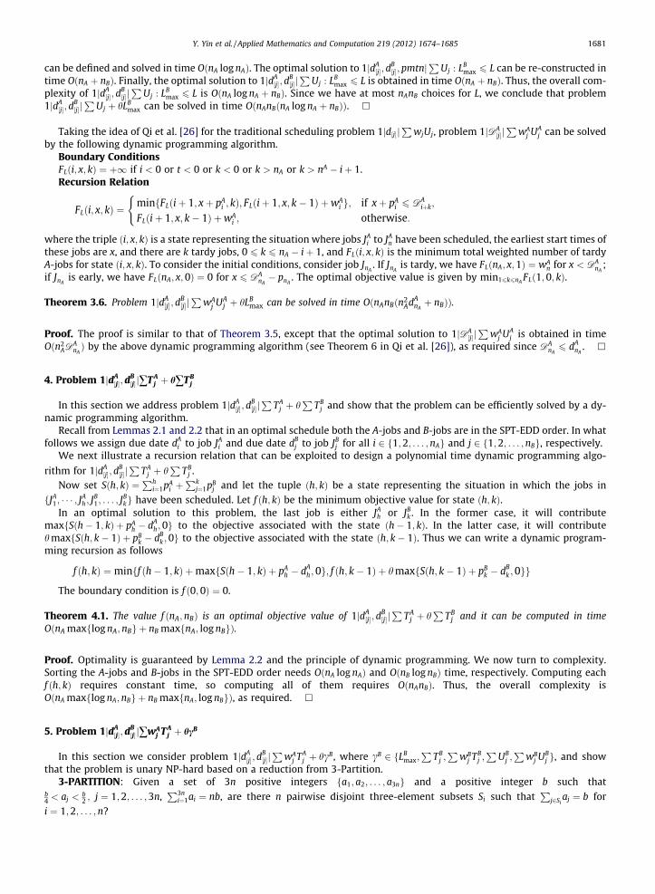
Taking the idea of Qi et al. [26] for the traditional scheduling problem 1jd½j�jP

wjUj, problem 1jDA½j�jP

wAj UA

j can be solvedby the following dynamic programming algorithm.

Boundary ConditionsFLði; x; kÞ ¼ þ1 if i < 0 or t < 0 or k < 0 or k > nA or k > nA � iþ 1.Recursion Relation

FLði; x; kÞ ¼minfFLðiþ 1; xþ pA

i ; kÞ; FLðiþ 1; x; k� 1Þ þwAi g; if xþ pA

i 6 DAiþk;

FLðiþ 1; x; k� 1Þ þwAi ; otherwise:

(

where the triple ði; x; kÞ is a state representing the situation where jobs JAi to JA

n have been scheduled, the earliest start times ofthese jobs are x, and there are k tardy jobs, 0 6 k 6 nA � iþ 1, and FLði; x; kÞ is the minimum total weighted number of tardyA-jobs for state ði; x; kÞ. To consider the initial conditions, consider job JnA

. If JnAis tardy, we have FLðnA; x;1Þ ¼ wA

n for x < DAnA

;if JnA

is early, we have FLðnA; x; 0Þ ¼ 0 for x 6 DAnA� pnA

. The optimal objective value is given by min16k6nAFLð1;0; kÞ.


B½j�jP

wAj UA

j þ hLBmax can be solved in time OðnAnBðn2

AdAnAþ nBÞÞ.

Proof. The proof is similar to that of Theorem 3.5, except that the optimal solution to 1jDA½j�jP

wAj UA

j is obtained in timeOðn2

ADAnAÞ by the above dynamic programming algorithm (see Theorem 6 in Qi et al. [26]), as required since DA

nA6 dA

nA. h


B½j� j+TA

j þ h+TBj

In this section we address problem 1jdA½j�; d

B½j�jP

TAj þ h

PTB

j and show that the problem can be efficiently solved by a dy-namic programming algorithm.

Recall from Lemmas 2.1 and 2.2 that in an optimal schedule both the A-jobs and B-jobs are in the SPT-EDD order. In whatfollows we assign due date dA

i to job JAi and due date dB

j to job JBj for all i 2 f1;2; . . . ;nAg and j 2 f1;2; . . . ;nBg, respectively.

We next illustrate a recursion relation that can be exploited to design a polynomial time dynamic programming algo-

rithm for 1jdA½j�; d

B½j�jP

TAj þ h

PTB

j .Now set Sðh; kÞ ¼

Phi¼1pA

i þPk

j¼1pBj and let the tuple ðh; kÞ be a state representing the situation in which the jobs in

fJA1; � � � ; J

Ah ; J

B1; . . . ; JB

kg have been scheduled. Let f ðh; kÞ be the minimum objective value for state ðh; kÞ.In an optimal solution to this problem, the last job is either JA

h or JBk . In the former case, it will contribute

maxfSðh� 1; kÞ þ pAh � dA

h ;0g to the objective associated with the state ðh� 1; kÞ. In the latter case, it will contributeh maxfSðh; k� 1Þ þ pB

k � dBk ;0g to the objective associated with the state ðh; k� 1Þ. Thus we can write a dynamic program-

ming recursion as follows

f ðh; kÞ ¼minff ðh� 1; kÞ þmaxfSðh� 1; kÞ þ pAh � dA

h ;0g; f ðh; k� 1Þ þ h maxfSðh; k� 1Þ þ pBk � dB

k ;0gg

The boundary condition is f ð0;0Þ ¼ 0.

Theorem 4.1. The value f ðnA;nBÞ is an optimal objective value of 1jdA½j�; d

B½j�jP

TAj þ h

PTB

j and it can be computed in timeOðnA maxflog nA;nBg þ nB maxfnA; log nBgÞ.

Proof. Optimality is guaranteed by Lemma 2.2 and the principle of dynamic programming. We now turn to complexity.Sorting the A-jobs and B-jobs in the SPT-EDD order needs OðnA log nAÞ and OðnB log nBÞ time, respectively. Computing eachf ðh; kÞ requires constant time, so computing all of them requires OðnAnBÞ. Thus, the overall complexity isOðnA maxflog nA;nBg þ nB maxfnA; log nBgÞ, as required. h


B½j� j+wA

j TAj þ hcB

In this section we consider problem 1jdA½j�; d

B½j�jP

wAj TA

j þ hcB, where cB 2 fLBmax;

PTB

j ;P

wBj TB

j ;P

UBj ;P

wBj UB

j g, and showthat the problem is unary NP-hard based on a reduction from 3-Partition.

3-PARTITION: Given a set of 3n positive integers fa1; a2; . . . ; a3ng and a positive integer b such thatb4 < aj <

b2 ; j ¼ 1;2; . . . ;3n,

P3ni¼1ai ¼ nb, are there n pairwise disjoint three-element subsets Si such that

Pj2Si

aj ¼ b fori ¼ 1;2; . . . ;n?



B½j�jP

wAj TA

j þ hcB is unary NP-hard.

Proof. We reduce 3-Partition to the problem 1jdA½j�; d

B½j�jP

wAj TA

j þ hcB6 Q . Given an instance of 3-Partition, we can construct

an instance of 1jdA½j�; d

B½j� jP

wAj TA

j þ hcB6 Q as follows:

nA ¼ 3n,pA

j ¼ aj; j ¼ 1;2; . . . ;3n,w A

j ¼ aj; j ¼ 1;2; . . . ;3n,

d Aj ¼ 0; j ¼ 1;2; . . . ;3n,

nB ¼ n� 1,pB

j ¼ 1; j ¼ 1;2; . . . ;n� 1,

dBj ¼ bþ 1; j ¼ 1;2; . . . ;n� 1,

w Bj ¼ 1; j ¼ 1;2; . . . ;n� 1,

Q ¼P

16i6j63naiaj þ nðn�1Þb2 ,

h ¼ Q þ 1.

Then the B-jobs can be viewed as the U-jobs in the instance constructed of the recognition version of problem

1jd½j�jP

wjTj. Analogous to the proof of Theorem 3 in Qi et al. [26], it is easy to see that problem 1jdA½j�; d

B½j�jP

wAj TA

j þ hcB6 Q

has a feasible solution if and only if there exists a feasible solution to 3-Partition, as required. h


B½j�j+wA

j UAj þ h+TB

j

In this section we show that problem 1jdA½j�; d

B½j�jP

wAj UA

j þ hP

TBj is binary NP-hard based on a reduction from Partition. We

then develop a pseudo-polynomial time dynamic programming algorithm for 1jdA½j�; d

B½j�jP

wAj UA

j þ hP

TBj .

PARTITION: Given a set of n positive integers fa1; a2; . . . ; ang and an integer b such thatPn

i¼1ai ¼ 2b, does there exist apartition of the index set f1;2; . . . ;ng into subsets S1 and S2, such that

Pi2S1

ai ¼ b ¼P

i2S2ai?


B½j�jP

wAj UA

j þ hP

TBj is binary NP-hard.

Proof. We reduce Partition to problem 1jdA½j�; d

B½j�jP

wAj UA

j þ hP

TBj 6 Q . Given an instance of Partition, we can construct an

instance of 1jdA½j�; d

B½j�jP

wAj UA

j þ hP

TBj 6 Q as follows:

nA ¼ n,p A

j ¼ aj; j ¼ 1;2; . . . ; n,w A

j ¼ aj; j ¼ 1;2; . . . ; n,

d Aj ¼ b; j ¼ 1;2; . . . ;n,

nB ¼ 1,pB

1 ¼ b,

dB1 ¼ 2b,

h ¼ bþ 1,Q ¼ b.

Now we show that problem 1jdA½j�; d

B½j�jP

wAj UA

j þ hP

TBj 6 Q has a feasible solution if and only if there exists a feasible

solution to Partition.Given a feasible solution S to 1jdA

½j�; dB½j�jP

wAj UA

j þ hP

TBj 6 Q , we prove that Partition is solvable. We first claim that job JB

1

must be early, i.e., TB1 ¼ 0, or else hTB

1 P bþ 1 > Q . Now let Se be the set of early A-jobs and St be the set of tardy A-jobs. ThenPJAj 2St

wAj ¼

PJAj 2St

aj 6 b, soP

JAj 2Se

wAj ¼ 2b�

PJAj 2St

aj P b. On the other hand, the total processing time of early A-jobs must

not exceed b, the common due date for all A-jobs. Therefore,P

JAj 2Se

pAj ¼

PJAj 2Se

aj 6 b. ThusP

JAj 2Se

aj ¼ b ¼P

JAj 2St

aj, which

implies that the sets Se and St represent a solution to Partition.Conversely, given a feasible solution to Partition, we prove that problem 1jdA

½j�; dB½j�jP

wAj UA

j þ hP

TBj 6 Q has a feasible

solution. Suppose that the sets S1 and S2 represent a solution to Partition. Consider the following schedule S: first schedulethe B-job to be processed during the interval ½b;2b�, then schedule the subsets S1 and S2 of the A-jobs in the intervals ½0; b� and½2b;3b�, respectively. Hence, the B-job JB

1 and all the A-jobs in S1 are early and all the A-jobs in S2 are tardy, while the

corresponding objective function value isP

wAj UA

j þ hTB1 ¼

Pj2S2

wAj ¼

Pj2S2

aj ¼ b. Therefore, schedule S is feasible for the

problem 1jdA½j�; d

B½j�jP

wAj UA

j þ hP

TBj 6 Q . h


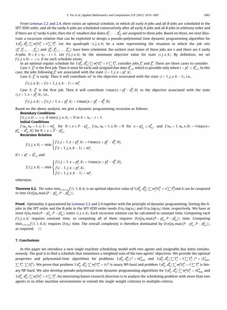
From Lemmas 2.2 and 2.4, there exists an optimal schedule, in which all early A-jobs and all B-jobs are scheduled in theSPT-EDD order, and all the tardy A-jobs are scheduled consecutively after all early A-jobs and all B-jobs in arbitrary order and

if there are nAt tardy A-jobs, then the nA

t smallest due dates dA1; � � � ; d

AnA

tare assigned to these jobs. Based on these, we next illus-

trate a recursion relation that can be exploited to design a pseudo-polynomial time dynamic programming algorithm for

1jdA½j�; d

B½j�jP

wAj UA

j þ hP

TBj . Let the quadruple ði; j; x; kÞ be a state representing the situation in which the job sets

fJAi ; J

Aiþ1; . . . ; JA

nAg and fJB

j , JBjþ1; . . . ; JB

nBg have been scheduled, the earliest start times of these jobs are x and there are k tardy

A-jobs, 0 6 k 6 nA � iþ 1. Let f ði; j; x; kÞ be the minimum objective value for state ði; j; x; kÞ. By definition, we setf ði; j; x; kÞ ¼ þ1 if no such schedule exists.

In an optimal regular schedule for 1jdA½j�; d

B½j�jP

wAj UA

j þ hP

TBj , consider jobs JA

i and JBj . There are three cases to consider.

Case 1: JAi is the first job. Then it must be early and assigned due date dA

iþk, which is possible only when t þ pAi 6 dA

iþk. In thiscase, the jobs following JA

i are associated with the state ðiþ 1; j; xþ pAi ; kÞ.

Case 2: JAi is tardy. Then it will contribute wA

i to the objective associated with the state ðiþ 1; j; x; k� 1Þ, i.e.,

f ði; j; x; kÞ ¼ f ðiþ 1; j; x; k� 1Þ þwAi :

Case 3: JBj is the first job. Then it will contribute h maxfxþ pB

j � dBj ; 0g to the objective associated with the state

ði; jþ 1; xþ pBj ; kÞ, i.e.,

f ði; j; x; kÞ ¼ f ði; jþ 1; xþ pBj ; kÞ þ h maxfxþ pB

j � dBj ;0g:

Based on the above analysis, we give a dynamic programming recursion as follows:Boundary Conditionsf ði; j; x; kÞ ¼ þ1 if minfi; j; x; kg < 0 or k > nA � iþ 1.Initial Conditionsf ðnA;nB þ 1; x;1Þ ¼ wA

nAfor 0 6 x 6 P � pA

nA, f ðnA;nB þ 1; x;0Þ ¼ 0 for xþ pA

nA6 dA

nA, and f ðnA þ 1;nB; x;0Þ ¼ h maxfxþ

pBnB� dB

nB;0g for 0 6 x 6 P � pB

nB.

Recursion Relation

f ði; j; x; kÞ ¼minf ði; jþ 1; xþ pB

j ; kÞ þ h maxfxþ pBj � dB

j ;0g;f ðiþ 1; j; x; k� 1Þ þwA

i ;

(

if t þ pAi > dA

iþk and

f ði; j; x; kÞ ¼minf ði; jþ 1; xþ pB

j ; kÞ þ h maxfxþ pBj � dB

j ;0g;f ði� 1; j; xþ pA

i ; kÞ;f ðiþ 1; j; x; k� 1Þ þwA

i ;

8><>:

otherwise.

Theorem 6.2. The value min16k6nAf ð1;1;0; kÞ is an optimal objective value of 1jdA

½j�; dB½j�jP

wAj UA

j þ hP

TBj and it can be computed

in time Oðn2AnB maxfP � pA

nA; P � pB

nBgÞ.

Proof. Optimality is guaranteed by Lemmas 2.2 and 2.4 together with the principle of dynamic programming. Sorting the A-jobs in the SPT order and the B-jobs in the SPT-EDD order needs OðnA log nAÞ and OðnB log nBÞ time, respectively. We have atmost n2

AnB maxfP � pAnA; P � pB

nBg states ði; j; x; kÞ. Each recursion relation can be calculated in constant time. Computing each

f ði; j; x; kÞ requires constant time, so computing all of them requires Oðn2AnB maxfP � pA

nA; P � pB

nBgÞ time. Computing

min16k6nAf ð1;1;0; kÞ requires OðnBÞ time. The overall complexity is therefore dominated by Oðn2

AnB maxfP � pAnA; P � pB

nBgÞ,

as required. h

7. Conclusions

In this paper we introduce a new single-machine scheduling model with two agents and assignable due dates simulta-neously. The goal is to find a schedule that minimizes a weighted sum of the two agents’ objectives. We provide the optimal

properties and polynomial-time algorithms for problems 1jdA½j�; d

B½j�jcA þ hLB


B½j�jP

TAj þ h

PTB

j ; cA 2 fLAmax;P

TAj ;P

UAj g. We prove that problem 1jdA

½j�; dB½j�jP

wAj TA

j þ hcB is unary NP-hard and problem 1jdA½j�; d

B½j�jP

wAj UA

j þ hP

TBj is bin-

ary NP-hard. We also develop pseudo-polynomial-time dynamic programming algorithms for 1jdA½j�; d

B½j�jP

wAj UA

j þ hLBmax and

1jdA½j�; d

B½j�jP

wAj UA

j þ hP

TBj . An interesting future research direction is to analyze the scheduling problem with more than two

agents or in other machine environments or extend the single weight criterion to multiple-criteria.


Acknowledgements

We are grateful to the Editor and three anonymous referees for their constructive comments on an earlier version of ourpaper. This paper was supported in part by the Natural Science Foundation for Young Scholars of Jiangxi, China(2010GQS0003); in part by the NSC of Taiwan under Grant No. NSC 100-2221-E-035-032; and in part by NSC of Taiwan un-der Grant No. NSC 101-2410-H-264-004.

References

[1] A. Agnetis, P.B. Mirchandani, D. Pacciarelli, A. Pacifici, Scheduling problems with two competing agents, Operations Research 52 (2004) 229–242.[2] A. Agnetis, D. Pacciarelli, A. Pacifici, Multi-agent single machine scheduling, Annals of Operations Research 150 (2007) 3–15.[3] A. Agnetis, G. Pascale, D. Pacciarelli, A Lagrangian approach to single-machine scheduling problems with two competing agents, Journal of Scheduling

12 (2009) 401–415.[4] K.R. Baker, J.C. Smith, A multiple criterion model for machine scheduling, Journal of Scheduling 6 (2003) 7–16.[5] T.C.E. Cheng, S.-R. Cheng, W.-H. Wu, P.-H. Hsu, C.-C. Wu, A two-agent single- machine scheduling problem with truncated sum-of-processing-times-

based learning considerations, Computers & Industrial Engineering 60 (2011) 534–541.[6] T.C.E. Cheng, M.C. Gupta, Survey of scheduling research involving due-date determination decisions, European Journal of Operational Research 38

(1989) 156–166.[7] T.C.E. Cheng, C.T. Ng, J.J. Yuan, Multi-agent scheduling on a single machine to minimize total weighted number of tardy jobs, Theoretical Computer

Science 362 (2006) 273–281.[8] T.C.E. Cheng, C.T. Ng, J.J. Yuan, Multi-agent scheduling on a single machine with max-form criteria, European Journal of Operational Research 188

(2008) 603–609.[9] T.C.E. Cheng, W.-H. Wu, S.-R. Cheng, C.-C. Wu, Two-agent scheduling with position-based deteriorating jobs and learning effects, Applied Mathematics

and Computation 217 (2011) 8804–8824.[10] V.S. Gordon, J.M. Proth, C. Chu, Due date assignment and scheduling: SLK, TWK and other due date assignment models, Production Planning and

Control 13 (2002) 117–132.[11] V.S. Gordon, J.M. Proth, C. Chu, A survey of the state-of-the-art of common due date assignment and scheduling research, European Journal of

Operational Research 139 (2002) 1–25.[12] V. Gordon, V. Strusevich, A. Dolgui, Scheduling with due date assignment under special conditions on job processing, Journal of Scheduling (2010),

http://dx.doi.org/10.1007/s10951-011-0240-2.[13] N.G. Hall, Scheduling problems with generalized due dates, IIE Transactions 18 (1986) 220–222.[14] C.J. Hsu, S.J. Yang, D.L. Yang, Two due date assignment problems with position-dependent processing time on a single-machine, Computers & Industrial

Engineering 60 (2011) 796–800.[15] V. Lauff, F. Werner, Scheduling with common due date, earliness and tardiness penalties for multimachine problems: a survey, Mathematical and

Computer Modelling 40 (2004) 637–655.[16] H.-T. Lee, D.L. Yang, S.-J. Yang, Multi-machine scheduling with deterioration effects and maintenance activities for minimizing the total earliness and

tardiness costs, International Journal of Advanced Manufacturing Technology (2012), http://dx.doi.org/10.1007/ s00170- 012-4348-0.[17] K. Lee, B.C. Choi, J.Y.T. Leung, M.L. Pinedo, Approximation algorithms for multi-agent scheduling to minimize total weighted completion time,

Information Processing Letters 109 (2009) 913–917.[18] J.Y.T. Leung, M.L. Pinedo, G. Wan, Competitive two-agent scheduling and its applications, Operations Research 58 (2) (2010) 458–469.[19] P. Liu, L.X. Tang, X.Y. Zhou, Two-agent group scheduling with deteriorating jobs on a single machine, International Journal of Advanced Manufacturing

Technology 47 (2010) 657–664.[20] P. Liu, N. Yi, X.Y. Zhou, Two-agent single-machine scheduling problems under increasing linear deterioration, Applied Mathematical Modelling 35

(2011) 2290–2296.[21] Y.-Y. Lu, G. Li, Y.-B. Wu, J. Ping, Optimal due-date assignment problem with learning effect and resource-dependent processing times, Optimization

Letters (2012), http://dx.doi.org/10.1007/s11590-012-0467-7.[22] B. Mor, G. Mosheiov, Scheduling problems with two competing agents to minimize minmax and minsum earliness measures, European Journal of

Operational Research 206 (2010) 540–546.[23] B. Mor, G. Mosheiov, Single machine batch scheduling with two competing agents to minimize total flowtime, European Journal of Operational

Research 215 (2011) 524–531.[24] G. Mosheiov, D. Oron, Due-date assignment and maintenance activity scheduling problem, Mathematical and Computer Modelling 44 (2006) 1053–

1057.[25] C.T. Ng, T.C. E Cheng, J.J. Yuan, A note on the complexity of the two-agent scheduling on a single machine, Journal of Combinatorial Optimization 12

(2006) 387–394.[26] X.T. Qi, G. Yu, J.F. Bard, Single machine scheduling with assignable due dates, Discrete Applied Mathematics 122 (2002) 211–233.[27] R. Rudek, The strong NP-hardness of the maximum lateness minimization scheduling problem with the processing-time based aging effect, Applied

Mathematics and Computation 218 (2012) 6498–6510.[28] D. Shabtay, Scheduling and due date assignment to minimize earliness, tardiness, holding, due date assignment and batch delivery costs, International

Journal of Production Economics 123 (2010) 235–242.[29] C. Sriskandarajah, A note on the generalized due dates scheduling problems, Naval Research Logistics 37 (1990) 587–597.[30] K. Tanaka, M. Vlach, Single machine scheduling to minimize the maximum lateness with both specific and generalized due dates, IEICE Transactions on

Fundamentals of Electronics, Communications and Computer Sciences 80 (1997) 557–563.[31] K. Tanaka, M. Vlach, Minimizing maximum absolute lateness and range of lateness under generalized due dates on a single machine, Annals of

Operations Research 86 (1999) 507–526.[32] G. Wan, R.S. Vakati, J.Y.T. Leung, M.L. Pinedo, Scheduling two agents with controllable processing times, European Journal of Operational Research 205

(2010) 528–539.[33] J.-B. Wang, M.Z. Wang, Single machine multiple common due dates scheduling with learning effects, Computers and Mathematics with Applications 60

(2010) 2998–3002.[34] J.B. Wang, Q. Guo, A due-date assignment problem with learning effect and deteriorating jobs, Applied Mathematical Modelling 34 (2010) 309–313.[35] X.-Y. Wang, M.-Z. Wang, Single machine common flow allowance scheduling with a rate-modifying activity, Computers and Industrial Engineering 59

(2010) 898–902.[36] J.-B. Wang, C.-M. Wei, Parallel machine scheduling with a deteriorating maintenance activity and total absolute differences penalties, Applied

Mathematics and Computation 217 (2011) 8093–8099.[37] S.-J. Yang, Single-machine scheduling problems with both start-time dependent learning and position dependent aging effects under deteriorating

maintenance consideration, Applied Mathematics and Computation 217 (2010) 3321–3329.[38] S.-J. Yang, C.J. Hsu, D.-L. Yang, Single-machine scheduling and slack due-date assignment with aging effect and deteriorating maintenance,

Optimization Letters (2011), http://dx.doi.org/10.1007/s11590-011-0382-3.

http://dx.doi.org/10.1007/s10951-011-0240-2

http://dx.doi.org/10.1007/s00170-012-4348-0

http://dx.doi.org/10.1007/s11590-012-0467-7

http://dx.doi.org/10.1007/s11590-011-0382-3


[39] Y. Yin, S.-R. Cheng, C.-C. Wu, Scheduling problems with two agents and a linear non-increasing deterioration to minimize earliness penalties,Information Sciences 189 (2012) 282–292.

[40] Y. Yin, S.-R. Cheng, T.C.E. Cheng, W.-H. Wu, C.-C. Wu, Two-agent single-machine scheduling with release times and deadlines, International Journal ofShipping and Transport Logistics, forthcoming.

[41] J.J. Yuan, W.P. Shang, Q. Feng, A note on the scheduling with two families of jobs, Journal of Scheduling 8 (2005) 537–542.

Documents

Two-agent single-machine scheduling with assignable due dates