Embed Size (px)
DESCRIPTION
2d and 3d supersonic aerodynamics flow
Citation preview
FLOW IN TWO AND THREE DIMENSIONS
FLOW IN TWO AND THREE DIMENSIONS
The analysis previously given for one-dimensional flow are exactly correct only for the flow through an infinitesimal stream tube. For all real problems the assumption of one-dimensionality for the entire flow is at best an approximation. In many instances, especially those relating to the flow in ducts, the one- dimensional treatment is adequate. In other cases, however, the one-dimensional methods
FLOW IN TWO AND THREE DIMENSIONS
are not only inadequate but often can provide no information whatsoever about important aspects of the flow. This bring to importance of study of two and three dimensional flow.
To treat general case of three dimensional motion including friction, heat transfer, shocks, and a fluid with complex equation of state-involves mathematical difficulties so great that these can not be handled easily. Hence, it is necessary to conceive simple models of the flow which lend themselves to analytical treatment, but which at the same time furnish information of value concerning the real, and more complex, flow patterns. One of these approach is of using Prandtl’s concept of the boundary layer. This concept is well verified by experiment. In this concept it is possible to ignore friction and heat transfer for the region of potential flow outside of the boundary layer.
FLOW IN TWO AND THREE DIMENSIONS
According to this concept shearing stresses and heat transfer may be ignored compared to other effects, except in a thin film near solid boundaries. Thus the flow is assumed to be adiabatic and frictionless outside a boundary layer. In other words potential flow exist outside the boundary layer and it is independent of boundary layer.
POTENTIAL FLOW
Potential flow is(1) Irrotational(2) Adiabatic(3) Without Friction
THE PHYSICAL SIGNIFICANT OF IRROTATIONAL MOTION
Irrotational flow makes the flow equations simple to handle. Fluid rotation is defined as the average angular velocity of two mutually perpendicular differential elements in the fluid. In order to find an analytical expression for the fluid rotation at a point in two dimensional flow, let us consider the infinitesimal and mutually perpendicular fluid lines OA and OB of the figure shown on the next slid.
THE PHYSICAL SIGNIFICANT OF IRROTATIONAL MOTION
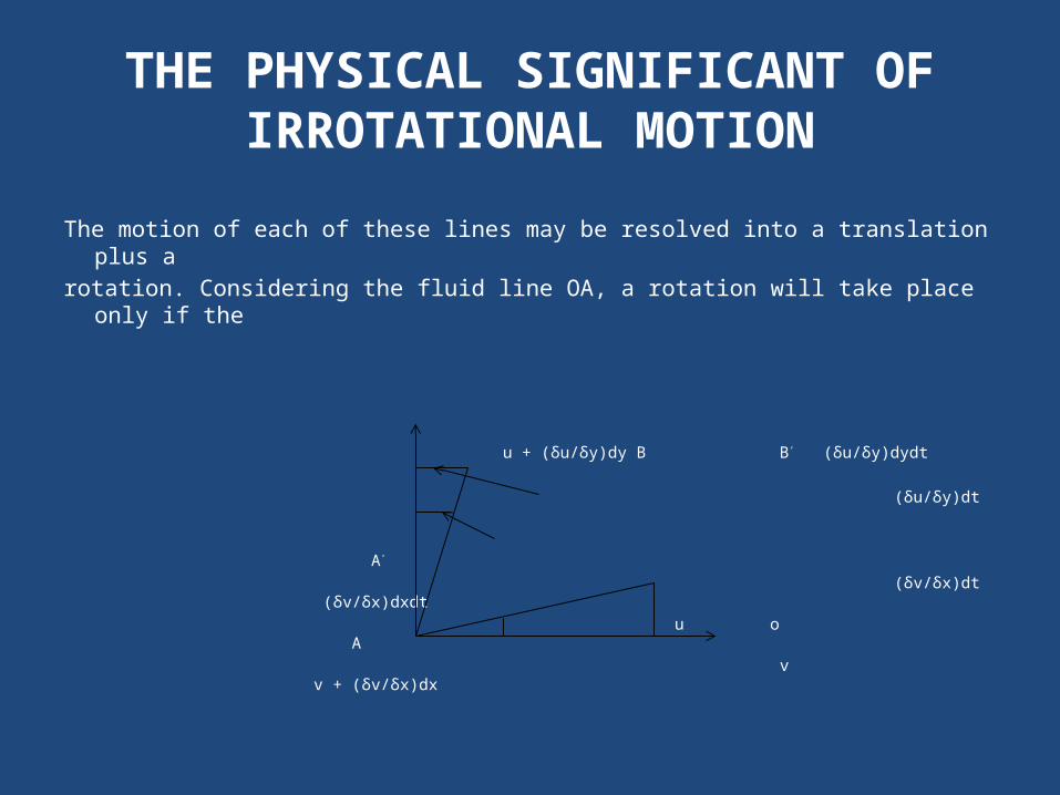
The motion of each of these lines may be resolved into a translation plus a rotation. Considering the fluid line OA, a rotation will take place only if the
u + (δu/δy)dy B B’ (δu/δy)dydt (δu/δy)dt
A’ (δv/δx)dt (δv/δx)dxdt u o A v v + (δv/δx)dx
THE PHYSICAL SIGNIFICANT OF IRROTATIONAL MOTION
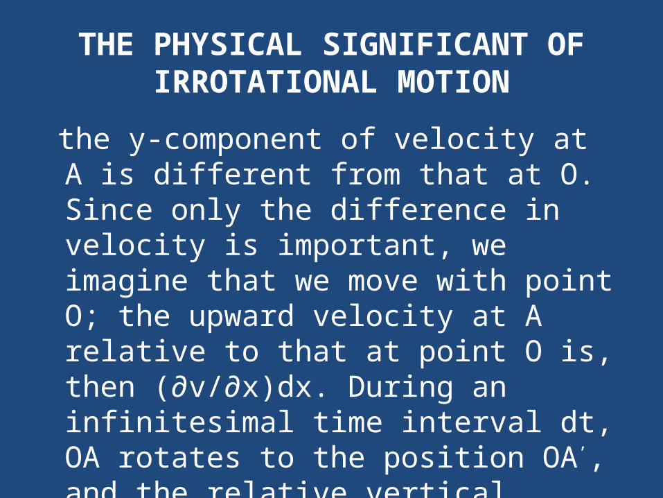
the y-component of velocity at A is different from that at O. Since only the difference in velocity is important, we imagine that we move with point O; the upward velocity at A relative to that at point O is, then (∂v/∂x)dx. During an infinitesimal time interval dt, OA rotates to the position OA’, and the relative vertical displacement AA’ = (∂v/∂x)dxdt
THE PHYSICAL SIGNIFICANT OF IRROTATIONAL MOTION
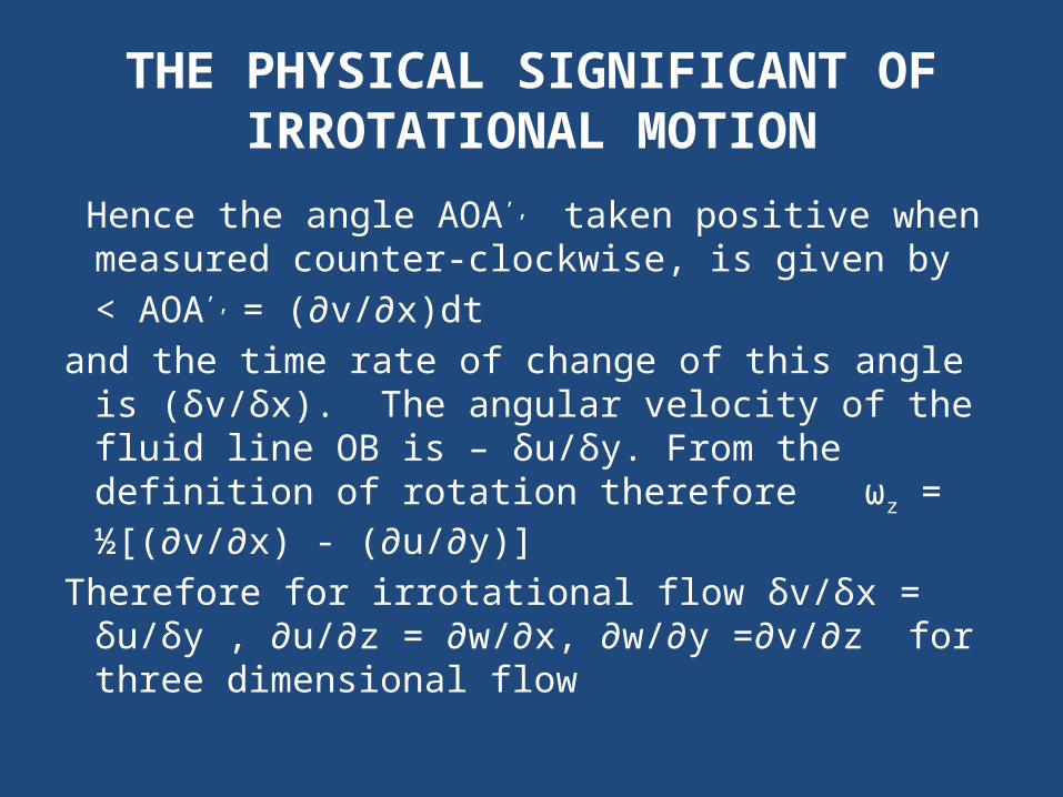
Hence the angle AOA’, taken positive when measured counter-clockwise, is given by< AOA’, = (∂v/∂x)dt
and the time rate of change of this angle is (δv/δx). The angular velocity of the fluid line OB is – δu/δy. From the definition of rotation therefore ωz = ½[(∂v/∂x) - (∂u/∂y)]
Therefore for irrotational flow δv/δx = δu/δy , ∂u/∂z = ∂w/∂x, ∂w/∂y =∂v/∂z for three dimensional flow
THE PHYSICAL SIGNIFICANT OF IRROTATIONAL MOTION
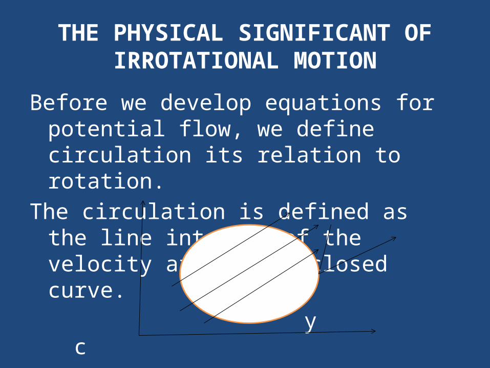
Before we develop equations for potential flow, we define circulation its relation to rotation.
The circulation is defined as the line integral of the velocity around any closed curve.
y c vcosα v
Referring to the closed c of fig.
THE PHYSICAL SIGNIFICANT OF IRROTATIONAL MOTION
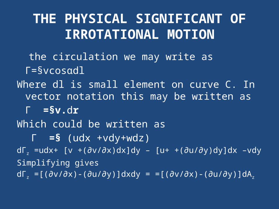
the circulation we may write asГ=§vcosαdl
Where dl is small element on curve C. In vector notation this may be written asГ =§v.dr
Which could be written as Г =§ (udx +vdy+wdz)
dГz =udx+ [v +(∂v/∂x)dx]dy – [u+ +(∂u/∂y)dy]dx –vdySimplifying gives dГz =[(∂v/∂x)-(∂u/∂y)]dxdy = =[(∂v/∂x)-(∂u/∂y)]dAz

THE PHYSICAL SIGNIFICANT OF IRROTATIONAL MOTION
The circulation per unit area in the x,y-plane is therefore dГz / dAz = ∂v/∂x-∂u/∂ y
Comparing rotation of the fluid with its circulation, we see that the circulation per unit area is twice the average rotation of a fluid particle
dГz / dAz = 2ωz
THE PHYSICAL SIGNIFICANT OF IRROTATIONAL MOTION
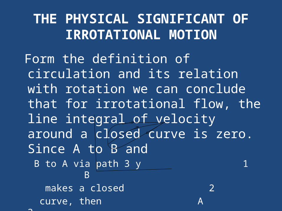
Form the definition of circulation and its relation with rotation we can conclude that for irrotational flow, the line integral of velocity around a closed curve is zero. Since A to B and
B to A via path 3 y 1 B makes a closed 2 curve, then A 3 ∫1A
B Vcosαdl +∫3B
A Vcosαdl =0 x
THE PHYSICAL SIGNIFICANT OF IRROTATIONAL MOTION
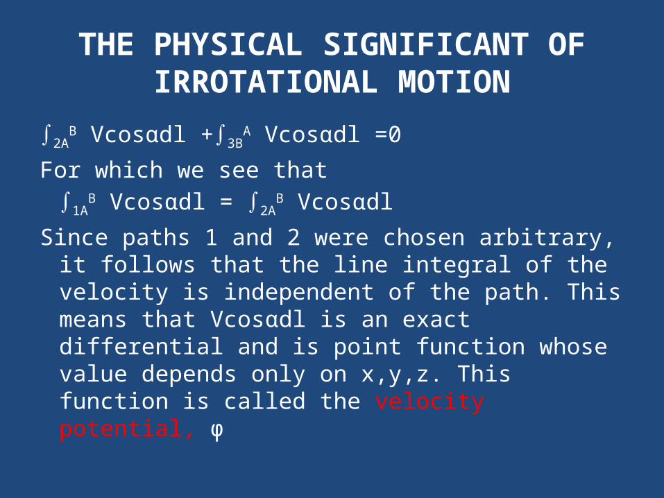
∫2AB Vcosαdl +∫3B
A Vcosαdl =0For which we see that
∫1AB Vcosαdl = ∫2A
B Vcosαdl Since paths 1 and 2 were chosen arbitrary, it follows
that the line integral of the velocity is independent of the path. This means that Vcosαdl is an exact differential and is point function whose value depends only on x,y,z. This function is called the velocity potential, φ
THE PHYSICAL SIGNIFICANT OF IRROTATIONAL MOTION
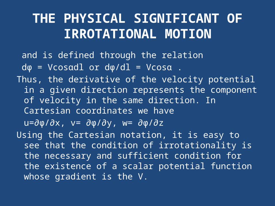
and is defined through the relation dφ = Vcosαdl or dφ/dl = Vcosα .Thus, the derivative of the velocity potential in a given
direction represents the component of velocity in the same direction. In Cartesian coordinates we haveu=∂φ/∂x, v= ∂φ/∂y, w= ∂φ/∂z
Using the Cartesian notation, it is easy to see that the condition of irrotationality is the necessary and sufficient condition for the existence of a scalar potential function whose gradient is the V.
THE PHYSICAL SIGNIFICANT OF IRROTATIONAL MOTION
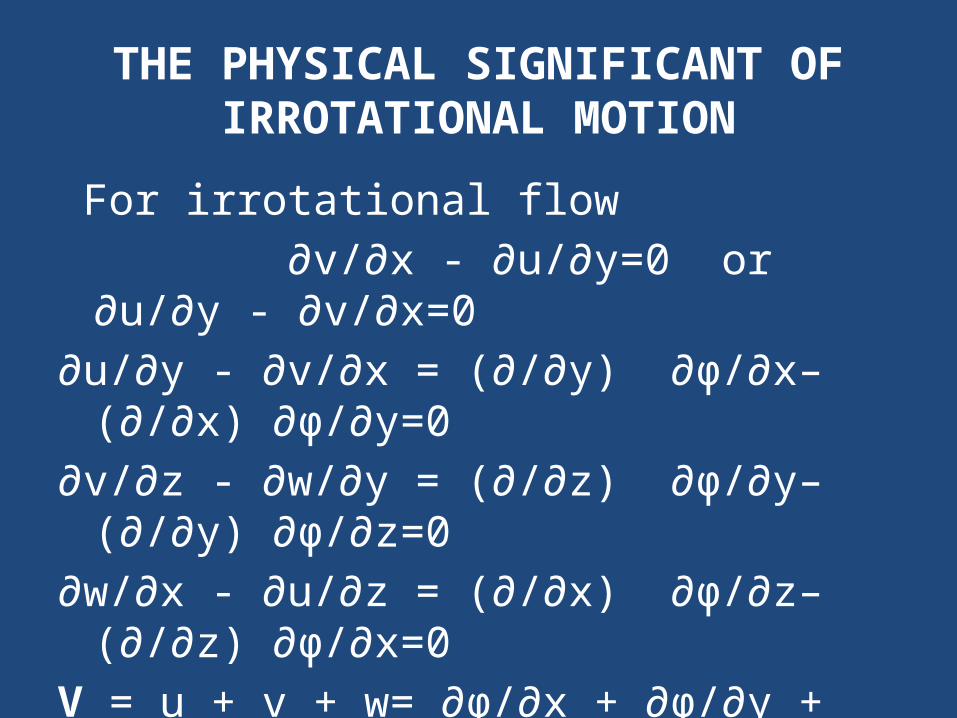
For irrotational flow ∂v/∂x - ∂u/∂y=0 or ∂u/∂y - ∂v/∂x=0∂u/∂y - ∂v/∂x = (∂/∂y) ∂φ/∂x– (∂/∂x) ∂φ/∂y=0∂v/∂z - ∂w/∂y = (∂/∂z) ∂φ/∂y– (∂/∂y) ∂φ/∂z=0∂w/∂x - ∂u/∂z = (∂/∂x) ∂φ/∂z– (∂/∂z) ∂φ/∂x=0V = u + v + w= ∂φ/∂x + ∂φ/∂y + ∂φ/∂zV = grad φ
THE DIFFERENTIAL EQUATION OF THE VELOCITY POTENTIAL
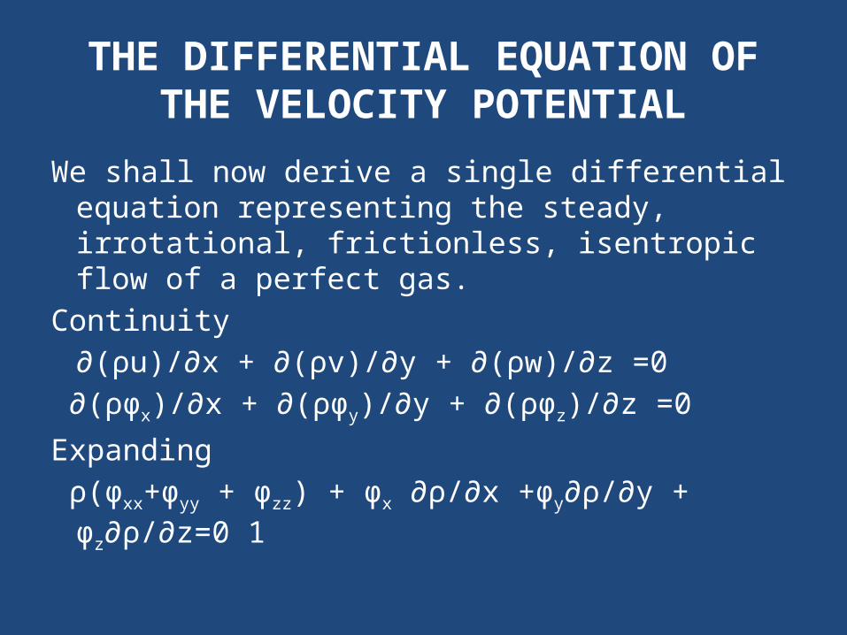
We shall now derive a single differential equation representing the steady, irrotational, frictionless, isentropic flow of a perfect gas.
Continuity∂(ρu)/∂x + ∂(ρv)/∂y + ∂(ρw)/∂z =0
∂(ρφx)/∂x + ∂(ρφy)/∂y + ∂(ρφz)/∂z =0Expanding ρ(φxx+φyy + φzz) + φx ∂ρ/∂x +φy∂ρ/∂y + φz∂ρ/∂z=0 1
THE DIFFERENTIAL EQUATION OF THE VELOCITY POTENTIAL
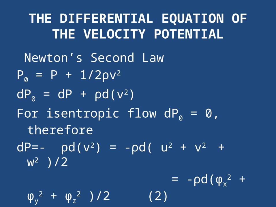
Newton’s Second LawP0 = P + 1/2ρv2
dP0 = dP + ρd(v2)For isentropic flow dP0 = 0, thereforedP=- ρd(v2) = -ρd( u2 + v2 + w2 )/2 = -ρd(φx
2 + φy2 + φz
2 )/2 (2)The sound velocity a2=(∂p/∂ρ)2
THE DIFFERENTIAL EQUATION OF THE VELOCITY POTENTIAL
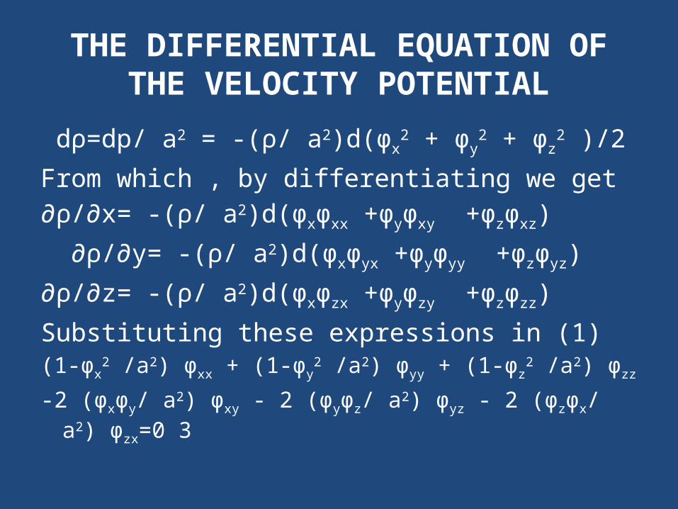
dρ=dp/ a2 = -(ρ/ a2)d(φx2 + φy
2 + φz2 )/2
From which , by differentiating we get∂ρ/∂x= -(ρ/ a2)d(φxφxx +φyφxy +φzφxz) ∂ρ/∂y= -(ρ/ a2)d(φxφyx +φyφyy +φzφyz)∂ρ/∂z= -(ρ/ a2)d(φxφzx +φyφzy +φzφzz)Substituting these expressions in (1)(1-φx
2 /a2) φxx + (1-φy2 /a2) φyy + (1-φz
2 /a2) φzz -2 (φxφy/ a2) φxy - 2 (φyφz/ a2) φyz - 2 (φzφx/ a2) φzx=0 3
THE DIFFERENTIAL EQUATION OF THE VELOCITY POTENTIAL
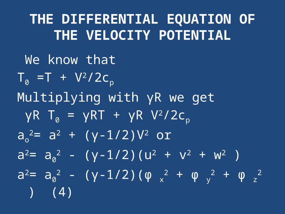
We know thatT0 =T + V2/2cp Multiplying with γR we get γR T0 = γRT + γR V2/2cp ao
2= a2 + (γ-1/2)V2 or a2= a0
2 - (γ-1/2)(u2 + v2 + w2 )a2= a0
2 - (γ-1/2)(φ x2 + φ y
2 + φ z2 ) (4)
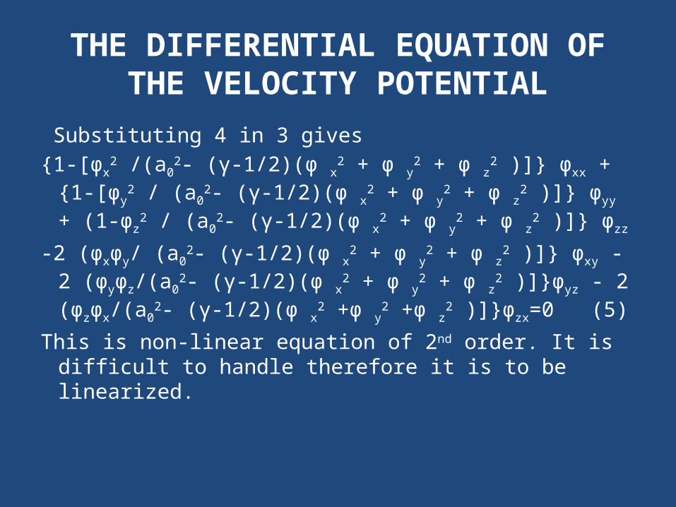
THE DIFFERENTIAL EQUATION OF THE VELOCITY POTENTIAL
Substituting 4 in 3 gives{1-[φx
2 /(a02- (γ-1/2)(φ x
2 + φ y2 + φ z
2 )]} φxx + {1-[φy2 /
(a02- (γ-1/2)(φ x
2 + φ y2 + φ z
2 )]} φyy + (1-φz2 / (a0
2- (γ-1/2)(φ x
2 + φ y2 + φ z
2 )]} φzz -2 (φxφy/ (a0
2- (γ-1/2)(φ x2 + φ y
2 + φ z2 )]} φxy - 2
(φyφz/(a02- (γ-1/2)(φ x
2 + φ y2 + φ z
2 )]}φyz - 2 (φzφx/(a02-
(γ-1/2)(φ x2 +φ y
2 +φ z2 )]}φzx=0 (5)
This is non-linear equation of 2nd order. It is difficult to handle therefore it is to be linearized.
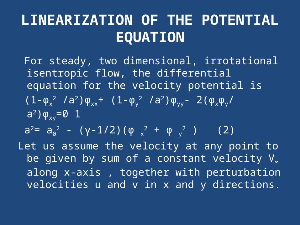
LINEARIZATION OF THE POTENTIAL EQUATION
For steady, two dimensional, irrotational isentropic flow, the differential equation for the velocity potential is
(1-φx2 /a2)φxx+ (1-φy
2 /a2)φyy- 2(φxφy/ a2)φxy=0 1 a2= a0
2 - (γ-1/2)(φ x2 + φ y
2 ) (2)Let us assume the velocity at any point to be given by
sum of a constant velocity V∞ along x-axis , together with perturbation velocities u and v in x and y directions.
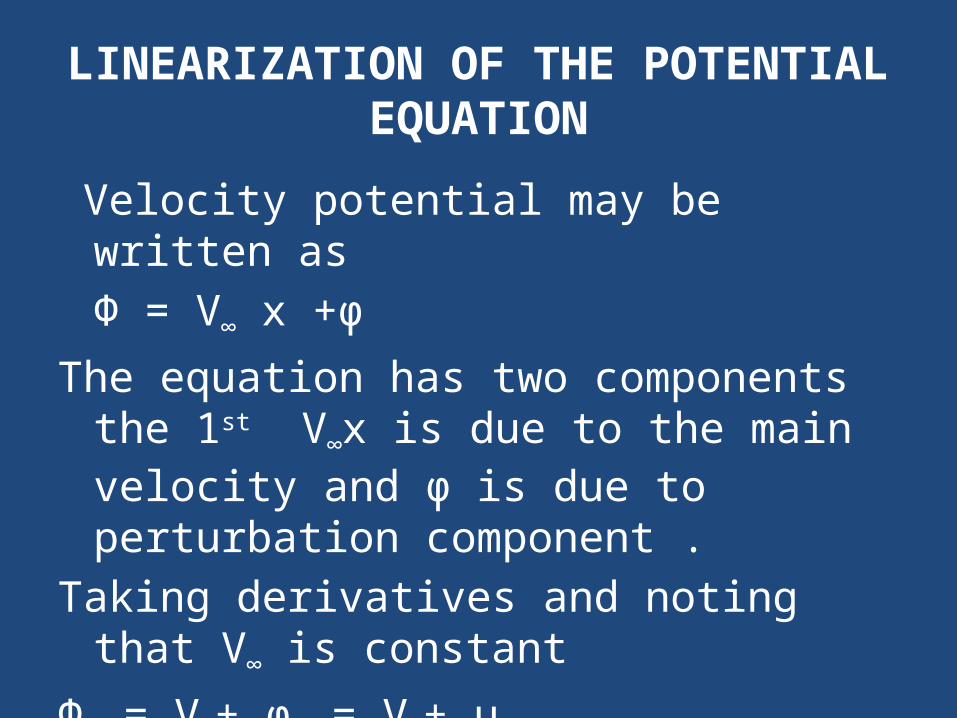
LINEARIZATION OF THE POTENTIAL EQUATION
Velocity potential may be written asФ = V∞ x +φ
The equation has two components the 1st V∞x is due to the main velocity and φ is due to perturbation component .
Taking derivatives and noting that V∞ is constantФx = V∞+ φx = V∞+ uФxx = φxx = ux
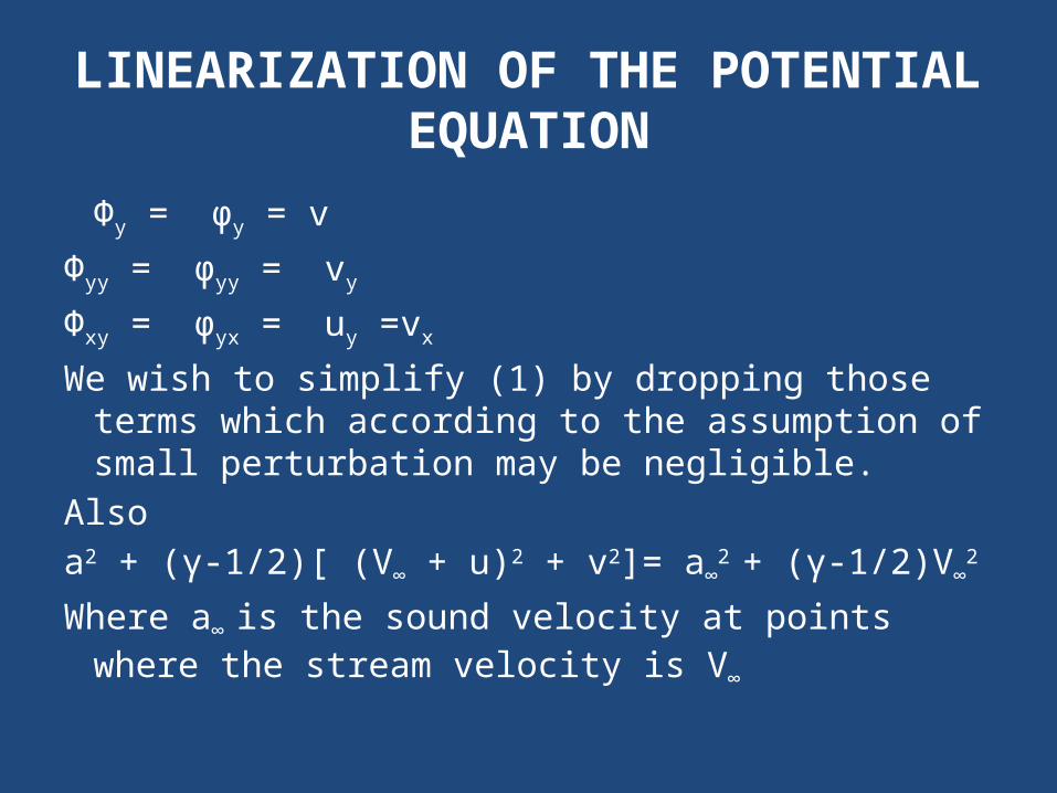
LINEARIZATION OF THE POTENTIAL EQUATION
Фy = φy = vФyy = φyy = vy
Фxy = φyx = uy =vx
We wish to simplify (1) by dropping those terms which according to the assumption of small perturbation may be negligible.
Alsoa2 + (γ-1/2)[ (V∞ + u)2 + v2]= a∞
2 + (γ-1/2)V∞
2
Where a∞ is the sound velocity at points where the stream velocity is V∞
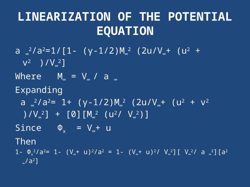
LINEARIZATION OF THE POTENTIAL EQUATION
a ∞2/a2=1/[1- (γ-1/2)M∞
2 (2u/V∞+ (u2 + v2 )/V∞
2]Where M∞ = V∞ / a ∞ Expanding a ∞
2/a2= 1+ (γ-1/2)M∞2 (2u/V∞+ (u2 + v2
)/V∞2] + [0]
[M∞2 (u2/ V∞
2)]Since Фx = V∞+ uThen1- Фx
2/a2= 1- (V∞+ u)2/a2 = 1- (V∞+ u)2/ V∞2][ V∞
2/ a ∞2][a2 ∞/a2]
LINEARIZATION OF THE POTENTIAL EQUATION
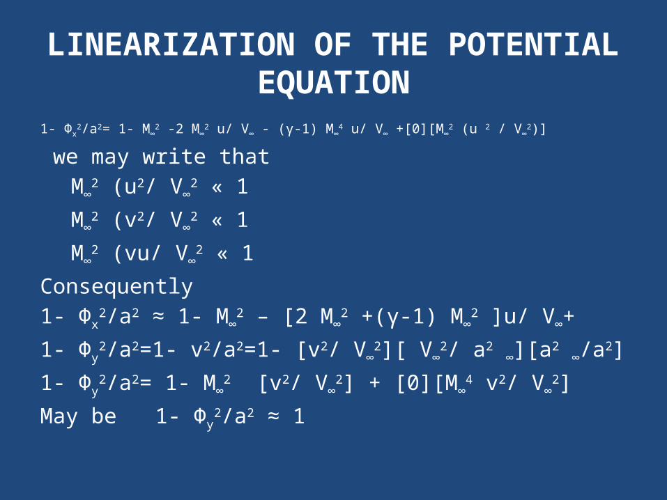
1- Фx2/a2= 1- M∞
2 -2 M∞2 u/ V∞ - (γ-1) M∞
4 u/ V∞ +[0][M∞2 (u 2 / V∞
2)]
we may write that M∞
2 (u2/ V∞2 « 1
M∞2 (v2/ V∞
2 « 1 M∞
2 (vu/ V∞2 « 1
Consequently1- Фx
2/a2 ≈ 1- M∞2 – [2 M∞
2 +(γ-1) M∞2 ]u/ V∞+
1- Фy2/a2=1- v2/a2=1- [v2/ V∞
2][ V∞2/ a2 ∞][a2 ∞/a2]
1- Фy2/a2= 1- M∞
2 [v2/ V∞2] + [0][M∞
4 v2/ V∞2]
May be 1- Фy2/a2 ≈ 1
LINEARIZATION OF THE POTENTIAL EQUATION
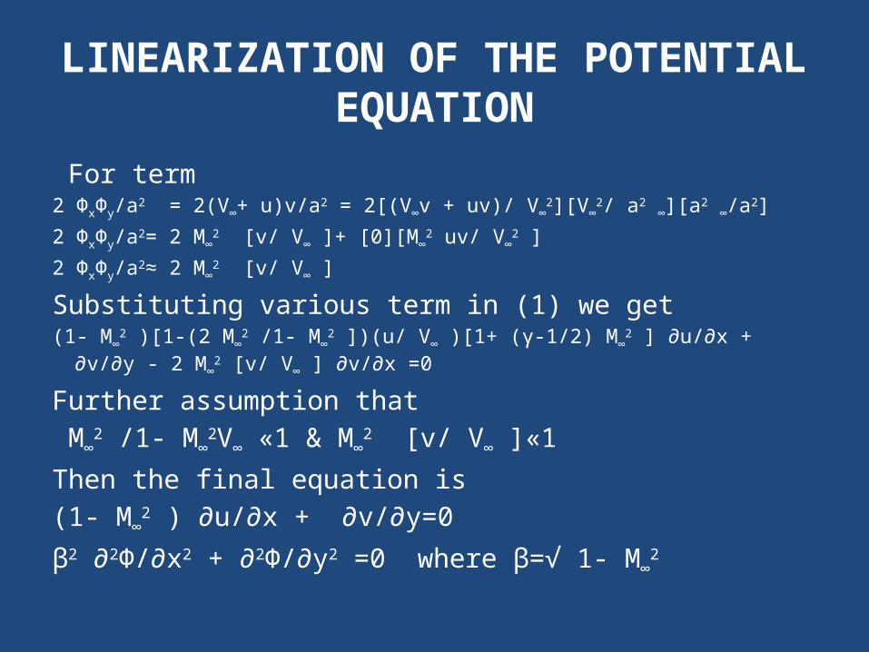
For term 2 ФxФy/a2 = 2(V∞+ u)v/a2 = 2[(V∞v + uv)/ V∞
2][V∞2/ a2 ∞][a2 ∞/a2]
2 ФxФy/a2= 2 M∞2 [v/ V∞ ]+ [0][M∞
2 uv/ V∞2 ]
2 ФxФy/a2≈ 2 M∞2 [v/ V∞ ]
Substituting various term in (1) we get(1- M∞
2 )[1-(2 M∞2 /1- M∞
2 ])(u/ V∞ )[1+ (γ-1/2) M∞2 ] ∂u/∂x + ∂v/∂y - 2 M∞
2 [v/ V∞ ] ∂v/∂x =0
Further assumption that M∞
2 /1- M∞2V∞ «1 & M∞
2 [v/ V∞ ]«1Then the final equation is(1- M∞
2 ) ∂u/∂x + ∂v/∂y=0β2 ∂2Ф/∂x2 + ∂2Ф/∂y2 =0 where β=√ 1- M∞
2