AEDC-TR-84-18 NOV 0 4 19~¢5

Two Approaches for the Prediction of Plume-Induced Separation

J. H. Fox Calspan Corporation, AEDC Division

April 1985

Final Report for Period October 1982 - January 1984

Property of U S. Air Force #.EGC LIBRARY

F40'300-81 -C-C004

TECHNICAL REPORTS FILE COPY

Approved for p.~bhc release; d=stnbutmn unlimited.

ARNOLD ENGINEERING DEVELOPMENT CENTER ARNOLD AIR FORCE STATION, TENNESSEE

AIR FORCE SYSTEMS COMMAND UNITED STATES AIR FORCE

NOTICES

When U. S. Government drawings, specifications, or other data are used for any purpose other than a definitely related Government procurement operation, the Government thereby incurs no responsibility nor any obligation whatsoever, and the fact that the government may have formulated, furnished, or in any way supplied the said drawings, specifications, or other data, is not to be regarded by implication or otherwise, or in any manner licensing the holder or any other person or corporation, or conveying any rights or permission to manufacture, use, or sell any patented invention that may in any way be related thereto.

Qualified users may obtain copies of this report from the Defense Technical Information Center.

References to named commercial products in this report are not to be considered in any sense as an endorsement of the product by the United States Air Force or the Government.

This report has been reviewed by the Office of Public Affairs (PA) and is releasable to the National Technical Information Service (NTIS). At NTIS, it will be available to the general public, including foreign nations.

APPROVAL S T A T E M E N T

This report has been reviewed and approved.

ROBERT H. NICHOLS Directorate of Technology Deputy for Operations

Approved for publicanon:

FOR THE COMMANDER

~ - C.~-" L . ~ > - - - ' 7 ~ • / f ~ 7 . , ~ . . , ~ ~ ~.~.,<~,e~...

MAI~ION L. LASTER Director of Technology Deputy for Operations

SECURPTY CLASSIFICATION OF THIS PAGE

REPORT DOCUMENTATION PAGE L t e R E P O R T S E C U R I T Y C L A S S I F I C A I l O N l b R E S T R I C T I V E M A R K I N G S

UNCLAS S I F I ED I l L I~ D S T R I B U T I O N / A V A I L A B I L T Y OF R E P O R T 2a SECU R I T V C L A S S I ~ : ~ C A T I O N ~ U T H O R I T Y

I L I Approved for public release; distri- :2b OECLASSIFICATION;DOWNGRADING SCHEDULE bution unlimited.

~4 P E R F C R M I N G O R G A N I Z A T [ O I % R E P O R T N U M B E R , S ;

AEDC-TR-84-18

6~i N A M E OF P E R F O R M I N G O R G A N I Z A T I O N

Arnold Engineering Development Center

,6¢ A D D R E S S (C i tv S t o r e a n d ZIP Code) i iAir Force Systems Command Arnold Air Force Station, I

5000 Ba N A M E OF F U N D I N G / S P O N S O R I N G

O R G A N I Z A T I O N A r n o l d F.. n .~ i -

nee-ring Development Center :8<: A D D R E S S ,C; tv :~f<ile =rid Z I P Code,

Sb O F F I C E S Y M B O L t l f app hcobLL'

i DOF

5 M O N = T O R I N G O R G A N I Z A T I O N R E P O R T N U M B E R ; S )

7a N A M E OF M O N I T O R I N G O R G A N I Z A T I O N

7b A D D R E S S {Ci ty 3 t a r e oncl Z I P C o d e r

TN 3 7 3 8 9 -

Sb O F F I C E S Y M B O L 9 P R O C U R E M E N T I N S T R U M E N T I D E N T I F I C A T I O N N U M B E R I I [ appl icable I

DOT

10 S O U R C E OF F I J N D i N G NOS

Air Force Systems Command Arnold Air Force Station, 5000

TN 3 7 3 8 9 - P R O G R A M I P R O J E C T I T A S K

E LE ME %1~" NO , NO NO ] I

1 T I T L E , I n t rude Securr ty Cta. t l l f lcat lor l ;

See I~everse of This Page 63370F

12 P E R S O N A L A U T H O R ( S I Fox, J'H., Calspan Corporation, AEDC Division

1 3 0 T Y P E OF R E P O R T 1 1 3 b T I M E C O V E R E D " 14 D A T E OF R E P O R T ( Y r "~]o Da>)

, Final I FROM ~0/I/82TOi i ~ April 1985 i i

1 6 S U P P L E M E N T A R Y N O T A T I O N

i Available in Defen.~e Technical Information Center (DTIC).

W O R K U N i T NO

15 PAGE C O U N T 58

17 C O S A T I C O D E S 1B S U B J E C T T E R M S ICnn t lnu¢ on reuer~*' I f qccesso~ and iden t t f y by b lock n u m ~ r )

F I E L D ] G R O U P I S U B GR I separation 16 1 04 i l Navier-Stokes equations 16 02 ~ computational fluid dynamics

tg . A B S T R A C T {ContJnue on ~uers~ J[ n e c e = s ~ ' ond ide~h [~ b> b lock nu ' , tb , "J

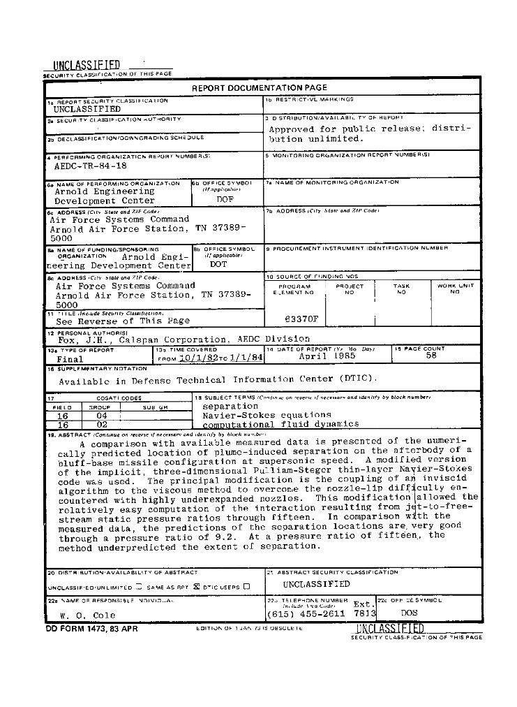
A comparison with available measured data is presented of the numeri- cally predicted location of plume-induced separation on the afterbody of a bluff-base missile configuration at supersonic speed. A modified version of the implicit, three-dimensional Pulliam-Steger thin-layer Navier-Stokes code was used. The principal modification is the coupling of an inviscid algorithm to the viscous method to overcome the nozzle-lip diff!cultv en- countered with highly underexpanded nozzles. This modification]allowed the relatively easy computation of the interaction resulting from j~t-to-free- stream static pressure ratios through fifteen. In comparison with the measured data, the predictions of the separation locations are very good through a pressure ratio of 9.2. At a pressure ratio of fifteen., the method underpredicted the extent of separation.

20 D t S T R I B U T I O N , A V A I L A B I L I T Y OF A B S T R A C T 2t A B S T R A C ' I S E C U R I T Y C L A S S I F I C A T I O N

UNCLASSIF'EO;UNLIMI"rED - - SAME AS R P T N DTIC USERS [] UNCLASSIFIED I I - - I

22a N A M E CF R E S P O N S I B L E N D I V I O ~ A ~ i /22~ TELEPHONEtn, t~de t ~.a C,Jde,NUMBER E x t .122, OFF CE S Y M B C L "1

W. O. Cole (615) 455-2611 78]~ DOS L I I

DO FORM 1473, 83 APR E D , T , O , ' , . JA0 . , 3 ,S OESOLETE UNCLASS I F I E D S E C U R I T Y C L A S S . F ~CAT ION OF T H I S P A G E

UNCLASSIFIED S E C U R I T Y C L A S S I F I C A T I O N OF T H I S PAGE

TITLE. Continued.

Two Approaches for the Prediction o f P l u m e - I n d u c e d S e p a r a t i o n

lVNCLASSIFIEII S E C U R I T Y C L A S S I F I C A T I O N OF T H I S PAGE

AEDC-TR-84-18

PREFACE

The work reported was conducted by the Arnold Engineering Development Center

(AEDC), Air Force Systems Command (AFSC), under AEDC Project No. D205PW. The analysis was done at the request of the AEDC Analysis and Evaluation Division (DOFA) for

AEDC/DOT. The AEDC/DOT project manager was Dr. Keith Kushman, and the

AEDC/DOFAA project manager was Mr. Russell B. Sorrells. The results were obtained by

Calspan Corporation, AEDC Division, operating contractor of the Aerospace Flight

Dynamics testing effort at the AEDC, AFSC, Arnold Air Force Station, Tennessee. The manuscript was submitted for publication on April 26, 1984.

AEDC-TR-84-18

C O N T E N T S

Page

1.0 I N T R O D U C T I O N ........................................................ 5

2.0 C O M P O N E N T M E T H O D

2.1 General .............................................................. 6

2.2 Basic Componen t Theory ............................................... 6

2.3 Extension o f Theory ................................................... 7

2.4 Mixing Theory . . . . . . . . . . . . . . . . . . . . . . . . . ' ............................... 7

2.5 Recompression ....................................................... 9

2.6 Conservation Equations o f the Base Flow ................................. 10

2.7 Initial Velocity Profile ................................................. 11

2.8 Computat ional Procedure .............................................. 11

2.9 Discussion o f Component Method Results ................................ 12

3.0 T H E NAVIER-STOKES A P P R O A C H

3.1 General .............................................................. 13

3.2 Basic Equations ....................................................... 14

3.3 Grid ................................................................. 17

3.4 Boundary Condit ions and Nozzle-Lip Artifice . . . . . . . . . . . . . . . . . . . . . . . . . . . . . 18

3.5 Turbulence Model ..................................................... 18

3.6 Turbulence Model Verification .......................................... 20

3.7 Computed Results and Comparisons with Measured Data . . . . . . . . . . . . . . . . . . . 21

4.0 CONCLUSIONS AND R E C O M M E N D A T I O N S . . . . . . . . . . . . . . . . . . . . . . . . . . . . . 24

REFERENCES ........................................................... 24

I L L U S T R A T I O N S

Figure

1. Schematic of Plume Interaction ............................................ 27

2. Interaction Showing Shear-Layer Model ............................... • . . . . 27

3. Details of Recompression Region .......................................... 28

4. Typical Separated Boundary-Layer Profile .................................. 29

5. Af te rbody Pressure Distribution, Component Method . . . . . . . . . . . . . . . . . . . . . . . . 30

6. Prediction of Separation Extent, Component Method . . . . . . . . . . . . . . . . . . . . . . . . . 31

7. Computat ional Grid ..................................................... 32

8. Schematic of Base Region ................................................. 33

9. Overlapping Grids ....................................................... 34

AEDC-TR-84-18

Figure P a g e

10. A R T Solid-St ing C o m p a r i s o n ............................................. 35

11. Pred ic t ion o f Sepa ra t ion Extent , Nav ie r -S tokes M e t h o d . . . . . . . . . . . . . . . . . . . . . . . 36

12. A f t e r b o d y Pressure Dis t r ibu t ion ........................................... 37

13. P la t eau Pressure C o m p a r i s o n ............................................. 40

14. Base Pressure C o m p a r i s o n ................................................ 41

15. Densi ty C o n t o u r , PE/Po. = 15.2 ........................................... 42

16. Pressure C o n t o u r , PE/P~. = 15.2 .......................................... 43

17. Dens i ty C o n t o u r , p z / p ~ = 6.0 ............................................ 44

18. Pressure C o n t o u r , p z / p ~ = 6.0 ........................................... 45

19. Velocity Vectors , pE/po * = 6.0 ............................................ 46

20. Velocity Vectors , P E / P ~ = 15.2 ........................................... 47

APPENDIX

A. T r a n s f o r m a t i o n to Curvi l inear Coord ina t e s .................................. 49

A. N O M E N C L A T U R E "; .,. 52

AEDC-TR 8 4 - 1 8

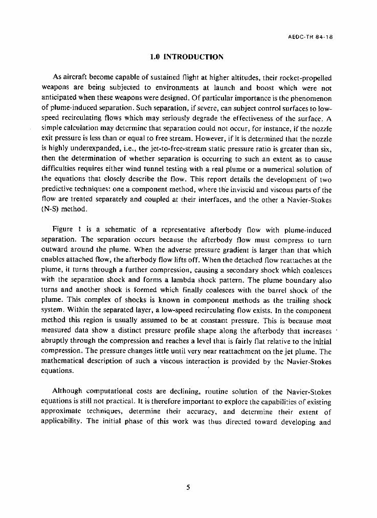
1.0 INTRODUCTION

As aircraft become capable of sustained flight at higher altitudes, their rocket-propelled

weapons are being subjected to environments at launch and boost which were not

anticipated when these weapons were designed. Of particular importance is the phenomenon

of plume-induced separation. Such separation, if severe, can subject control surfaces to low-

speed recirculating flows which may seriously degrade the effectiveness of the surface. A

simple calculation may determine that separation could not occur, for instance, if the nozzle

exit pressure is less than or equal to free stream. However, if it is determined that the nozzle

is highly underexpanded, i.e., the jet-to-free-stream static pressure ratio is greater than six, then the determination of whether separation is occurring to such an extent as to cause

difficulties requires either wind tunnel testing with a real plume or a numerical solution of

the equations that closely describe the flow. This report details the development of two

predictive techniques: one a component method, where the inviscid and viscous parts of the

flow are treated separately and coupled at their interfaces, and the other a Navier-Stokes (N-S) method.

Figure 1 is a schematic of a representative afterbody flow with plume-induced separation. The separation occurs because the afterbody flow must compress to turn

outward around the plume. When the adverse pressure gradient is larger than that which enables attached flow, the afterbody flow lifts off. When the detached flow reattaches at the

plume, it turns through a further compression, causing a secondary shock which coalesces with the separation shock and forms a lambda shock pattern. The plume boundary also

turns and another shock is formed which finally coalesces with the barrel shock of the

plume. This complex of shocks is known in component methods as the trailing shock system. Within the separated layer, a low-speed recirculating flow exists. In the component

method this region is usually assumed to be at constant pressure. This is because most

measured data show a distinct pressure profile shape along the afterbody that increases "

abruptly through the compression and reaches a level that is fairly flat relative to the initial compression. The pressure changes little until very near reattachment on the jet plume. The

mathematical description of such a viscous interaction is provided by the Navier-Stokes equations.

Although computational costs are declining, routine solution of the Navier-Stokes equations is still not practical. It is therefore important to explore the capabilities of existing approximate techniques, determine their accuracy, and determine their extent of applicability. The initial phase of this work was thus directed toward developing and

AEDC-TR-84-18

extending an existing component method that had proved to work well in predicting base

properties where separation on the afterbody was not present. A requirement arose,

however, for a predictive technique for vehicles at high angles of attack. The component methods are not applicable in these flows, because they require an external criterion for separation that is based on singular point separation, which is no longer valid in three-

dimensional flows (Ref. 1). This led to the modification of a three-dimensional N-S solver specifically to solve the plume-induced separation problem. This work with the N-S solver

allowed it to be brought into use when another drawback to the component method became apparent: at low free-stream Mach number and high jet-to-free-stream pressure ratios, the

external flow is forced to turn beyond the supersonic turning limit, causing a detached

normal shock. The component method was not formulated to account for mixed flows.

This report is of two parts. The first part presents the approach to developing the

component method into a tool for predicting plume-induced separation. The second part is

devoted to the modifications required of a three-dimensional N-S solver to make it useful

for predicting plume-induced separation at realistic jet-to-free-stream pressure ratios.

2.0 COMPONENT METHOD

2.1 GENERAL

The development of a component method capable of predicting plume-induced

separation is based on previous work, Refs. 2-4, which had generalized and extended the basic mixing and base flow theory of A. J. Chapman and H. H. Korst, Refs. 5-6, for

predicting base properties. This generalized theory was proved capable of predicting base flows, taking into account the boundary layer existing at separation, base bleed, and the

interaction of gas streams differing in chemistry and total enthalpy. Because of the wealth of

literature on this method, this report will dwell only on the changes required of the theory as

developed in Ref. 3.

2.2 BASIC COMPONENT THEORY

The basic component method based on Korst's work contains three distinct analyses: an inviscid analysis is used to determine the overall flow structure and the pressure field; a second analysis generates a set of integral conservation equations which describe the viscous

flow into and out of the base region; and the final analysis develops the mixing theory which produces the flow property profiles across the shear layers. Each of these analyses may be

developed independently. They are coupled in an iterative process. A solution to the base flow problem is achieved when the set of integral conservation equations is satisfied.

AEDC-TR-84-18

At any step in the iterative process, the base properties serve as boundary conditions to

the inviscid set of equations and to the mixing model. The base pressure adjusts the

boundaries ol the converging inviscid streams, the mixing theory locates thc mixing prolilcs

on the inviscid boundaries, and the integral conservation equations balance the cnergic,, and

mass rates into and out of the base region. The residual error of the integral conservation

equations drives the iteration process.

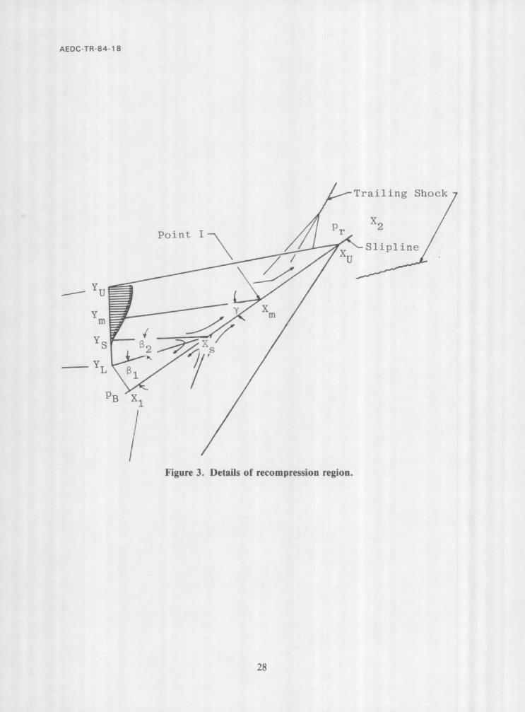
For the method to have closure, certain key streamlines must be located within the shear

layers, Figs. 2 and 3. The most difficult, historically, to determine is the stagnation

streamline, which determines what part of the converging shear layers will turn back toward

the base and what part will be turned downstream to experience recompres~ion. There are

many theories available for determining this streamline, all using empirical data to locate the

stagnation point. The methods of Refs. 3 and 4 use a minimum of empirical information to

develop a very workable theory that has been tested without change over a wide range of

flow configurations, including flows with enthalpy and chemistry differences at widely

different Math numbers. E

The coordinate systems used in the component method are sometimes confusing. The

general coordinate system is axially symmetric with X being the axial coordinate and R the

radial coordinate; however, the mixing layers have their own systcm. The coordinate along

the longitudinal direction of the shear layer is e; P = 0 at the point of separation. Y is the

coordinate normal to t, and X is the coordinate along the slip surface where the two streams

converge after separation (see Fig. 3).

2.3 EXTENSION OF THEORY

The analysis of Ref. 4 is extended in a straightforward manner to account for separation

occurring upstream of the base-afterbody juncture. This involves a modification Io the

inviscid flow solver (method of characteristics) to accommodate the separation shock ~.ave,

as illustrated in Fig. 2, and the inclusion of a separation criterion. Hahn, Ruppert, and

Mahal (Ref. 7) reviewed existing criteria extensively to determine when separation occurs.

For turbulent free-interaction separation, the authors suggest the criterion proposed b x,

Reshotko and Tucker

M2/MI = 0.762 (1)

That is, separation will occur when the ratio of the Mach number downstream of the

separation shock to that upstream of the shock is equal to 0.762. This criterion is

particularly easy to apply; however, its main drawback is that the separation on a boattail

af terbody is not truly of the free-interaction type. The upstream influence of the changing

curvature of the body is not taken into account. It would be expected that separation

AEDC-TR-84-18

predictions would be more accurate for large separations where the point of separation is

well up on the body.

2.4 MIXING THEORY

As shown in Fig. 2, the separated region is bounded by two shear layers which are assumed to converge at a slipline. The slipline is determined from the axially symmetric,

rotational method of characteristics (MOC). The method of characteristics is used also to

determine the inviscid, constant pressure boundaries of the separated region. At the inviscid

intersection, point I, the two mixing layers are assumed to have known velocity profiles:

[ ( l '-o 1 ,/p g'~l/ne _ ( ~ _ ,~p~.)2 d~" ~b = -~- 1 + erf ~7 - % " + ~ o (2)

where ~-l/n is the initial boundary-layer power-law profile and

aY 7 / - f

and

(3)

a~ r/p - (4)

/

where o is the mixing parameter. Equat ion (2) is the widely used error function profile distorted by the initial boundary layer. As the boundary-layer thickness goes to zero, the

second term becomes negligible. This occurs both when the separating boundary layer is very

thin and when the distance from separation to reat tachment is large, i.e., as e becomes large.

When r/p becomes small, the mixing layer is considered fully developed. The mixing parameter o is determined semiempirically. The method of Ref. 8 shows it to be well

approximated by

~D O ~b2d'q I' = | ou (5)

J ~L ICk ~, dr/ JOJ

where Ck is given as 0.5085/Oo. In the present work the incompressible ao is taken as 9.0.

Each profile at point I has the transverse coordinate 71 normal to its respective inviscid

boundary, increasing in value toward the high-speed stream. Following Ref. 6, the Y = 0

point is located by a m o m e n t u m balance as

IYu ou2dY [ I YU - ~'M = 0u2dy [

o g= o YL f (6)

AEDC-TR-84-18

This relation is solved for YM. This increment is the distance from the inviscid boundary to

the zero point of the profile. Thus this relation locates the profiles relative to their inviscid

boundaries. The edges of the mixing zones are somewhat arbitrary, but the points that have

worked well over many conditions are determined by the following:

1. Yu is located where the velocity is 99.998895 percent of the high-speed value.

2. YL is located at the point w, here the velocity is 0.001105 percent of the high-

speed value.

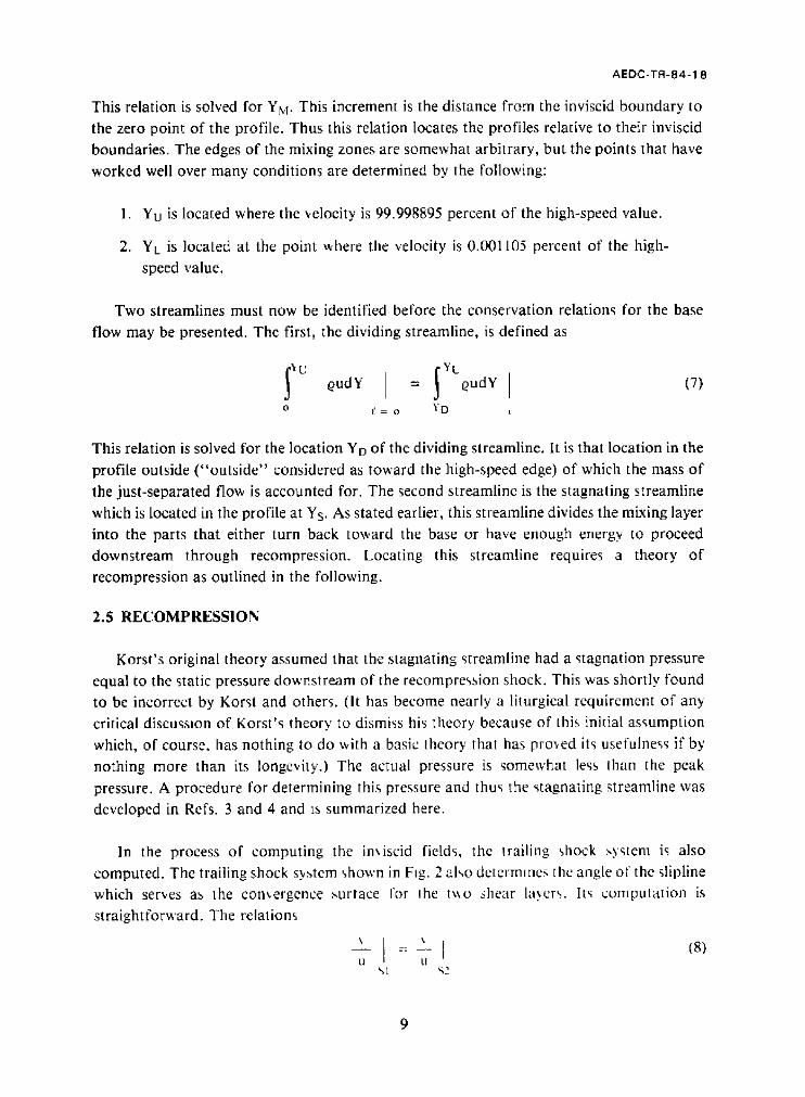
Two streamlines must now be identified before the conservation relations for the base

flow may be presented. The first, the dividing streamline, is defined as

l ~ U I YL ~udY = QudY

o I '= o YD

(7)

This relation is solved for the location Yo of the dividing streamline. It is that location in the

profile outside ("outs ide" considered as toward the high-speed edge) of which the mass of

the just-separated flow, is accounted for. The second streamlinc is the stagnating streamline

which is located in the profile at Ys. As stated earlier, this streamline divides the mixing layer

into the parts that either turn back tox~,ard the base or have enough energy to proceed

downstream through recompression. Locating this streamline requires a theory of

recompression as outlined in the following.

2.5 RECOMPRESSION

Korst's original theory assumed that the stagnating streamline had a stagnation pressure

equal to the static pressure downstream of the recompression shock. This was shortly found

to be incorrect by Korst and others. (It has become nearly a liturgical requirement of any

critical discussion of Korst's theory to dismiss his theory because of this initial assumption

which, of course, has nothing to do with a basic theory that has prm, ed its usefulness if by

nothing more than its longevity.) The actual pressure is somewhat less than the peak

pressure. A procedure for determining this pressure and thus the stagnating streamline was

developed in Refs. 3 and 4 and is summarized here.

In the process of computing the in~iscid fields, the trailing shock ,~ystem is also

computed. The trailing shock s~,~tem shown in Fig. 2 also determines the angle of the slipline

which ser~,es as the convergence ~urlace for 1he t~o shear la.~,ers. Its computation is

straightforward. The relations

[ ~ i (8) =-_- _ _ _ [

LI I LI

~,1 ":, ~

9

AEDC-TR-84-18

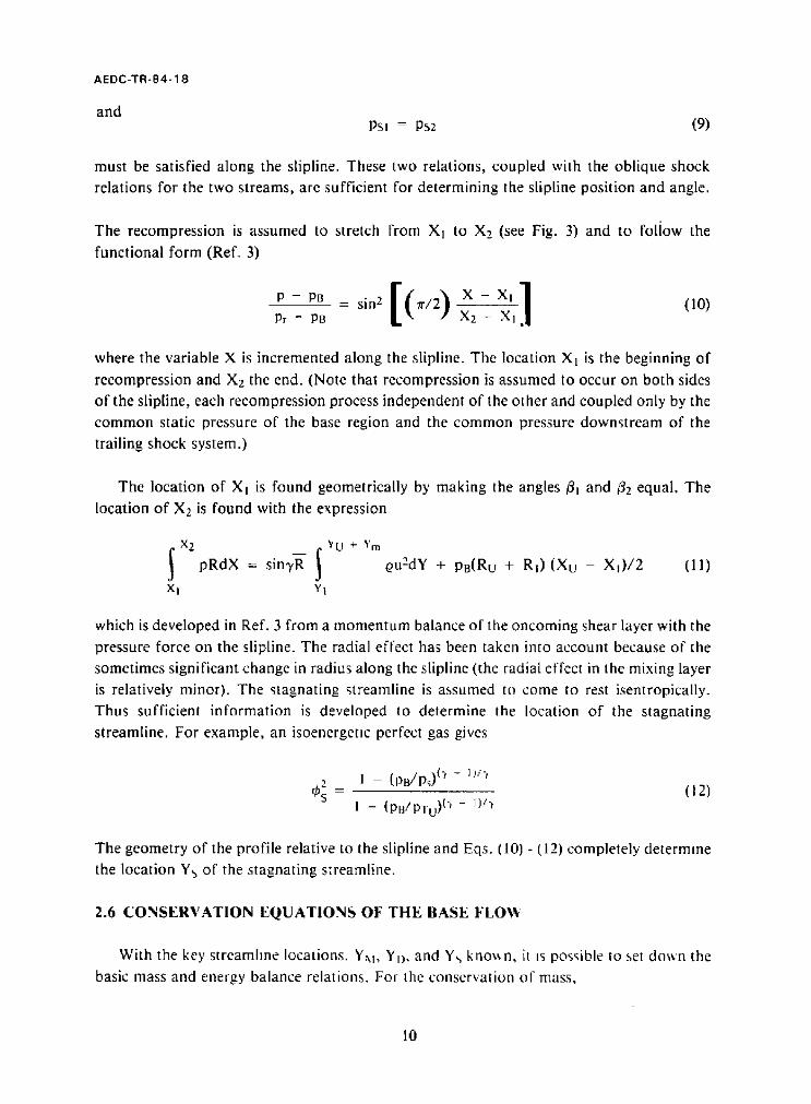
and PSI = P S 2 (9)

must be satisfied along the slipline. These two relations, coupled with the oblique shock

relations for the two streams, arc sufficient for determining the slipline position and angle.

The recompression is assumed to stretch from Xl to X2 (see Fig. 3) and to foliow the

functional form (Ref. 3)

P PB - sin z ~r/2 ,X'2 X'I P r - P8

(10)

where the variable X is incremented along the slipline. The location X1 is the beginning of

recompression and Xz the end. (Note that recompression is assumed to occur on both sides

of the slipline, each recompression process independent of the other and coupled only by the

common static pressure of the base region and the common pressure downstream of the

trailing shock system.)

The location of X~ is found geometrically by making the angles/31 and ~2 equal. The

location of X2 is found with the expression

X2 ~ U + Ym

XI YI

0u2dy + PB(Ru + RI ) (Xu - Xi) /2 (11)

which is developed in Ref. 3 from a momentum balance of the oncoming shear layer with the

pressure force on the slipline. The radial effect has been taken into account because of the

sometimes significant change in radius along the slipline (the radial effect in the mixing layer

is relatively minor). The stagnating streamline is assumed to come to rest isentropically.

Thus sufficient information is developed to determine the location of the stagnating

streamline. For example, an isoenergeuc perfect gas gives

, 1 - ( p B / p ~ ) ('r - l J/-r

~s = (12) 1 - ( p s / P T u ) [ ~ - 1)/-~

The geometry of the profile relative to the slipline and Eqs. (10) - (12) completely determine

the location Y~ of the stagnating streamline.

2.6 CONSERVATION EQUATIONS OF THE BASE FLO~'

With the key streamhne locations, Y,~h YI), and Y~, kno,,~ n, it is possible to set down the

basic mass and energy balance relations. For the conservation of mass,

10

AEDC-TR 8 4 - 1 8

I YD YD YS YS

YL SI YL $2 YL SI YL $2

(13)

and for energy,

o o ! ) I *s YL SI S2 SI 2 I[14)

These constitute the primary equations which are solved for the properties in the

base/separated region. Several auxiliary relations may be used when a species difference

exists between the exhaust gas and the free stream. These are found in Ref. 3 and are not

detailed here.

2.7 INITIAL VELOCITY PROFILE

The theory as developed in Refs. 3 - 4 assumed that the separating layer off a bluff base

would have a power-law profile. For separation occurring upstream of the base, the

separating profile is more closely related to the wake-like profile of a developing shear layer as shown in Fig. 4, using data from Refs. 9 - 10. This shape develops in a shear layer from an

initial power-law profile some distance downstream of a bluff edge. To more closely model the shape of the separating profile, the separating layer is assumed to separate with a profile

with % = 4.0. Thus, in the present calculations, it is assumed that the distance e has been

extended by a virtual amount. Thus the effective mixing length is

eef f ---- e q- ev]r (15)

where gvir = atS/4.0 (16)

2.8 COMPUTATIONAL PROCEDURE

Initial calculations were done using the GASL method of characteristics program, Ref. 11. This code was found to convect total pressure loss from the bow shock too far into the

field of the afterbody. This caused an overprediction of the extent of separation at higher

Mach numbers. The present results were calculated by assuming a constant pressure equal to the free-stream pressure from the shoulder of the missile to just upstream of the boattail break. Boundary-layer growth was then determined over this length using the method of

Ref. 12. The solution procedure is then as follows for isoenergetic flows:

11

AEDC-TR-84-18

. The MOC of Ref. 3 is started assuming free-stream conditions with no

boundary-layer displacement taken into account. This computation is marched

downstream to an assumed point of separation.

. A separation shock wave is computed and the MOC is continued. The

boundary on the edge of the separated region is determined by the guess of

pressure in that region. Computation of the plume field is also done with the

MOC. The intersection of the plume and outer stream is found and used to

determine the length of the inviscid boundaries.

3. The trailing shock system and slip surface are computed to obtain the peak

recompression pressure.

. The viscous mixing theory is then applied and the key streamlines are

determined. Finally, a mass balance of flow into and out of the separated

region is made.

If the mass balance equation is not satisfied, an error is determined, a new pressure is

calculated, and steps 2 through 4 are repeated. Once a converged separation pressure is

determined, the separation criterion for a turbulent boundary layer, Eq. (1), is used to

determine whether separation has occurred. If this condition is not satisfied, a new

separation point is assumed, and steps 1 through 4 are repeated. This continues until a

separation point is determined.

2.9 DISCUSSION OF COMPONENT METHOD RESULTS

Experimental data for afterbodies with a plume-induced separation are not widely

available. However, two reports of measured data that have appeared in the literature are

sufficient for validating the method as an engineering tool (Refs. 13 and 14). The results

from Ref. 13 are from a configuration run at a free-stream Mach number of 3.5 at various

static jet-to-free-stream pressure ratios. Comparisons are presented in Fig. 5 of predictions

made using the present component method with the measured data. Actual measured

separation points are not presented as they were not available; however, the predicted

separation point, which is indicated by the step rise in pressure, is located at a position

within the pressure rise that is consistent with the beginning of separation from other data

that are available, i.e., Ref. 14. They show separation occurring 10 to 20 percent into the

pressure rise. The calculated plateau pressure is high compared to the measured data. This is

because the predicted pressure is that which occurs downstream of an inviscid oblique shock

wave, which is of zero thickness. The measured pressure on the afterbody, however, is the

result of the smearing effect of the viscous layer, which spreads out the compression. The

peak pressure is thus pushed downstream, perhaps off the body.

12

AEDC-TR-84- 18

Comparison was made with the data of Ref: 14 at a lower Mach number. This

comparison is shown in Fig. 6. At the lower pressure ratios, the comparison is quite poor. In

general, the component method gives quite acceptable results at high jet-to-free-stream

pressure ratios where the separation is greater than three nozzle radii up the afterbody from

the base. This is expected since the external criterion used to determine when separation is

occurring is based on free interaction separation where separation is based only on local

conditions free from direct influences of downstream geometry such as the afterbody/base

juncture.

An anomalous condition sometimes occurs when trying to predict separation on bodies

where the Mach number of the outer stream is significantly lower than the Mach number of

the expanded jet boundary at the slipline. If the pressure ratio of the jet to free stream is

sufficiently high, then a solution to the trailing shock problem cannot be obtained because the outer stream is required to turn further than the oblique shock limit. That is, the

recompression shock on the plume boundary must be detached. This means that a subsonic

region exists downstream of the detached shock wave. The basic theory of this component

method does not account for such flows; therefore, this type of flow must be treated by

other methods, i.e., Navier-Stokes methods. This condition played substantially in the

decision to pursue the Navier-Stokes methods as discussed in the following.

3.0 THE NAVIERmSTOKES APPROACH

3.1 GENERAL

There are two principal reasons for exploring the use of N-S solvers for the solution of

the plume-induced separation problem:

1. The occurrence of the detached shock at the plume boundary with its attendant

subsonic region invalidates the component method because of its use of a

spatially hyperbolic inviscid solver (MOC). This happens when the two streams

are of substantially different Mach numbers.

2. A requirement for predictions at very high angles of attack (10 to 20 deg) also

invalidates the component method, because its externally applied separation

criterion is based on the occurrence of singular type separation, which does not

occur in general in three-dimensional flows.

A third, but less justifiable, reason is the fact that N-S solvers are conceptually pleasing because they use fewer empirically determined constructs. That element of the method

which does require empiricism, the modeling of the turbulent viscosity, shows signs of

becoming a rapidly maturing technology (Refs. 15 - 16).

13

AEDC-TR-84-18

When the N-S solver was used as detailed here, it became apparent early that extensive modification of the code would be required, if the extent of separation at any jet-to-free-

stream pressure ratio of interest was to be computed. The difficulty arises in the region just downstream of the nozzle lip. At high-pressure ratios, the barrel shock of the plume begins to form, developing a region of very high gradients. The expansion from the nozzle

overshoots, causing the local pressure to be lower than the ambient pressure. The flow must then be compressed sharply through the mechanism of the barrel shock to the boundary

pressure. The usual method of overcoming this type of problem is to either concentrate the computational mesh in this region or add additional smoothing or do both. The adding of points quickly reaches a limit when the available memory in the computer is exhausted and

the resolution of other important features of the flow is seriously degraded. Smoothing fails for an interesting reason. Smoothing effectively increases the viscosity in the high gradient

region. This has the effect of over-entraining fluid from the region of the base just above the

nozzle lip to the point that the pressure becomes unrealistically low, often to the point of being negative, causing the time-marching scheme to fail. If heroic measures are taken to

prevent the low pressure, the converged solution will often lack sufficient predictive accuracy. For these reasons, an artifice was developed to circumvent the nozzle-lip problem.

Because of the behavior of the algorithm in the nozzle-lip region and from experience

derived from development of the component model discussed earlier, the interaction at the nozzle lip was determined to be primarily inviscid. The nozzle lip is thus treated inviscidly

and removed from the region of the viscous solver. The inviscid MOC is used to develop new boundary conditions for the N-S solver downstream of the nozzle lip.

Results are presented of comparisons with available experimental data using this new procedure. A study using the same measured data for comparison was done by Deiwert,

Ref. 17. He used an azimuthally invariant form of the equations and a different gridding philosophy.

In the following, since the numerical tools are well developed and readily available in the open literature, many of the details will be referenced.

3.2 BASIC EQUATIONS

The three-dimensional, unsteady, thin-layer Navier-Stokes equations are transformed (see Appendix A) into the curvilinear coordinate system ~, r/, ~', and z as

14

AEDC-TR-84-18

where, with reference to Fig. 1, ~j is the body-conforming coordinate in the streamwise

direction, r/ is the body-conforming coordinate in the azimuthal direction, and g" is the outward coordinate ray from the body to the outermost boundary. The Cartesian x

coordinate is the axis of the body, the z coordinate is normal to x and tangent to the base of the body, and the x-z plane forms the slice used for presentation. Thus the Cartesian velocity

^ ^ ^

components of interest are u and w. The vectors q, E, F, and G are

~ U

~v Ow

e

0U 0uU + ~xP ~vU + ~ p

owU + ~zP (e + p)U - ~JtP

(18)

F = j - I

g = j - ,

0V 0uV + ~?xP 0vV + ~yP 0wV + ~/zP (e + p)V - rhP

G = j - I

0W 0uW + fxP 0vW + ~'yp 0wW + ~'zP (e + p ) W - ~'tp

0

/z(~-x2 + ~'~ + ~'2z)U ~. + (#/3)(~',u~. + ~'yv r + fzWr)~'x

#(fx2 + ~-~ + ~-2z)vr + (/~/3)(~'xu r + ~'yvr + g'zwr)~'r

#(~-2 x + ~-2y + ~-~)we + (td3)(~'xU ~- + fyV~ + ~'zW~-)fz

{(t-,2 + + -9[o.51,(u2 + v2 + w2).

+ k Pr -I (3' - l ) - l ( a 2 ) r ] + (#/3)(fxU + fyv + fzw)

×(Gut + ~'y v r + L wr)}

(19)

(20)

and the contravariant velocities are

U = ~ t + ~xu + ~yv + Gw

V = r/t + ~/x u + ~yV + ~/z w

W = ~'t + ~'x u + ~'yV + ~'z w

(21)

15

AEDC-TR-84-18

The pressure is determined f rom

p = (~ - l ) [e - 0 .50(u 2 + v 2 + w2)] (22)

and the Car tes ian velocity componen t s are non-dimensional ized with the free-s tream speed

of sound aoo; density 0 is scaled by 0o~; and the total energy, e, by 0o~a 2 .

The chain rule expansion o f derivatives o f the Cartesian coordinates with respect to the

curvilinear coordina tes is solved to give the metric terms

with

~x = J(Y.Zr - y~-zn)

= J ( z . x r - x . z : )

~z = J(x~y/- - y,rx~-)

~'x = J (YeZ~- z~yn)

= J(x, z - x z.)

~'z = J(xt/Yn - y~x~)

~x = J(z~y~- - y~z~-)

r/y = J(x~z~- - x~-z~)

7/z = J(y~x¢ - x~y~-)

~t = - XT~x - Y r~y - Z r~z

r/t = -- Xrr/x -- yrr/y -- Zrr/z

~'t = -- Xr~'x -- Yr~'y -- Zr~'z

(23)

j - I = xt y , z~- + x~- y~ z~ + x, y~- z~ - x~ y~- z~ - xn y~ z~- - x~- y~ z~ (24)

The approx imate factor izat ion difference equa t ion is

(I + h3~ ~n _ ~I J - 1 V~A~J)(I + h r , ]~n _ 6IJ- 1 V~A,IJ) X

(I + h6¢ (~n _ hRe-1 6~- j - l l~nJ _ el j - 1 Vra~.j)(qn+, _ ~n) (25)

= - At (0// IS n + 6 7 ~'n + Or (3. _ R e - 1 6/.Sn)

- - ~E j - 1 [ (V~A~)2 + (V~A~)2 + (V~.Af)2] Jcl n

where the 6's are the central-difference opera tors , A and V are fo rward and backward

dif ference opera tors , and h = t /2. The matrices A n, ]~n, a n d t~ n are ob ta ined f rom the

l inearization in time o f E n, Fn, and Gn. These are detailed by Pul l iam and Steger, Ref. 18,

a long with the coeff ic ient matrix 1~1 n. The smooth ing terms of the forms el J - 1 V~A~ Jcl and

16

AEDC-TR-84-18

eE J-1 (~'/~A//)2 Jcl are added specifically to damp nonlinear instabilities of the central

difference scheme.

This algorithm has been put into a practical code by Pulliam and Steger. The actual code

used herein is a vectorized form of Pulliam and Steger's code developed by J. A. Benek.

3.3 GRID

The development of a grid for the computational domain is perhaps as important as the solution algorithm itself. Because the thin-layer form of the conservation equations is being

used, certain physical assumptions are carried with any choice of grid.

The principal assumption made in the choice of grid is that the wake flow downstream of the base region including the plume may be treated as an inviscid, rotational flow. It is also assumed that the boundary layer in the nozzle has little effect on separation and may be

neglected. The effluent from the nozzle is thus treated as an inviscid, conical flow.

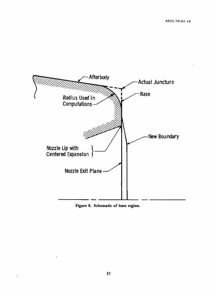
These basic assumptions lead to the backward " c " grid as shown in Fig. 7. By wrapping the afterbody/base region in a body-conforming coordinate, the basic code is left unchanged; concentrations of rays may be easily positioned at the nozzle lip region where resolution is most important, and the rays can be readily aligned with the plume boundary so that the reattachment point and the trailing shock system may be better resolved. Since the thin-layer assumption retains only those viscous terms in t.he conservation equations that have derivatives in the ~" direction and since the ~" coordinate is nearly aligned with the principal flow direction, the viscous terms effectively eliminated are in the region

downstream of the base/afterbody juncture.

The grid is wrapped in opposite directions away from the nozzle lip with an exponentially

increased spacing. A radius equal to 10 percent of the nozzle radius is added at the juncture of the base and the afterbody to smooth the grid around this corner. Axially symmetric flow is enforced by using five planes with identical boundary conditions. Five planes are required because of the fourth-order smoothing required for stability of the algorithm, Eq. (25). Early experimentation with underexpanded nozzles led to a device to avoid the singularity at the nozzle lip. Without extremely dense packing of points in the lip region, no flow with pressure ratios of significance could be computed. Consequently, the nozzle lip was eliminated from the region of computation for the viscous code. This was accomplished by adding a new surface extending from just above the nozzle lip to the nozzle centerline, as

shown in Fig. 8.

17

AEDC-TR-84-18

3.4 BOUNDARY CONDITIONS AND NOZZLE-LIP ARTIFICE

The Pulliam-Steger-Benek N-S solver uses explicit boundary conditions. While it is arguable that this type boundary condition impedes convergence, it nevertheless provides an

extremely practical code in which boundary conditions may be easily input or modified as were done on the new surface that avoids the nozzle-lip problem.

The boundary conditions on the new surface are provided by the MOCs (see Ref. 3), as

shown in Fig. 9. Beginning with the exit plane conditions, the steady, Euler-equations MOC is used to march an inviscid field out to the new boundary. The nozzle-lip singularity is

treated as a multivalued point using a Prandtl-Meyer centered expansion. The flow at the lip

is expanded until it reaches the pressure of the base point that is the intersection of the new

boundary and the base. As the base pressure changes continuously from initial conditions to the final converged solution, the expansion is adjusted with each time step. The boundary

conditions of the Navier-Stokes solver are thus being adjusted with each step. The boundary

conditions on the new surface that are imposed on the Navier-Stokes solver are obtained

from the characteristics by a double linear interpolation: i.e., the first interpolation is performed as the characteristics cross the new boundary, and the second is done to find the

flow properties at the fixed grid of the Navier-Stokes solver. The MOC develops its own grid from the initial spacing in the nozzle exit plane and from the number of pressure decrements through the expansion. So, a finer grid spacing in the nozzle exit plane or in the expansion will increase the resolution on the boundary for the N-S solver. A finer expansion grid is required for the higher pressure ratios.

The boundary conditions elsewhere are imposed in a straightforward manner. On the

body, the no-slip conditions are enforced with the contravariant velocities set to zero.

Density is imposed on the body as a first-order extrapolation from the first grid point off the body. Adiabatic wall conditions are enforced with the total energy, e, determined from the

zero pressure gradient condition normal to the wall. The upstream boundary-layer profile is taken from the experimental data. Free-stream conditions are imposed at the outer

boundary from the upstream boundary to the coordinate ray through the afterbody/base juncture, where the condition is changed to a zero-gradient outflow condition from that

point to the centerline. The conditions between the last streamline of the expansion fan and the base are obtained by first-order extrapolation from the field.

3.5 TURBULENCE MODEL

For N-S solvers to be useful in predicting flow behavior for practical configurations, they

require a turbulence model to relate properties of the flow field to the apparent change in

18

AEDC-TR-84-18

in viscosity caused by turbulence. The algebraic models are most attractive because of their

simplicity.

Baldwin and Lomax, Ref. 15, developed an algebraic turbulent viscosity model that is

widely used because of its favorable trade-off between ease of use and predictive accuracy in

unseparated flows. This model is a two-layer model with the inner mixing length proportional to the product of distance from the wall and the Van Driest damping factor. It

crosses over to a wake-type model in which the mixing length is scaled by the vorticity. According to Ref. 15, the model is valid for separated flows and, with the outer model

alone, for pure wakes. However, Thomas (Ref. 19) reports that if the outer model alone is used for wakes, instabilities develop, and that Baldwin, in private communication with Thomas, recommended using the basic two-layer model with minor adjustment. Thomas

proceeded, however, to develop his own variant. But for the present work, it was determined

from numerical experiments that the basic Baldwin-Lomax two-layer model, with minor

change, worked quite well.

The eddy viscosity is defined as

= oe2 I i (26)

near the body. It is defined in the wake as

eout = KCcp 0 Fwake Fkleb (Y) (27)

The inner model is switched over to the wake model when Ein = Eou t. The variable y here

refers to normal distance from the body and

and

where

Also,

+ (OzV- oyw) + (o w -

f = k y [ 1 - exp - y +

½ (28)

(29)

Y+ = Y [ (O'r-)~]# • (30)

wall

[ ( Ckleb ~'~61 -1 1 + 5.5 K Yma,~ / .~ Fkleb (Y) = (3l)

19

AEDC-TR-84-18

and

Fwake = Ymax Fmax (32)

o r

Fv, ake = Cv, k Ymax U~if Fmax

(33)

depending on which is the smaller. The terms Ymax and Fmax are determined from the

maximum of the function

Also,

F(y) = Y lo~ I [1 - exp - y +

Udi f = (U 2 -I- v 2 -I- W2) ½ - (U 2 d- V 2 -I- W2) ½.

(34)

(35)

Baldwin and Lomax assigned the following values to the parameters:

A + = 26.0

Ccp = 1.6

Ckleb = 0.3

Cwk = 0.25

k = 0.4

K = 0.0168

(36)

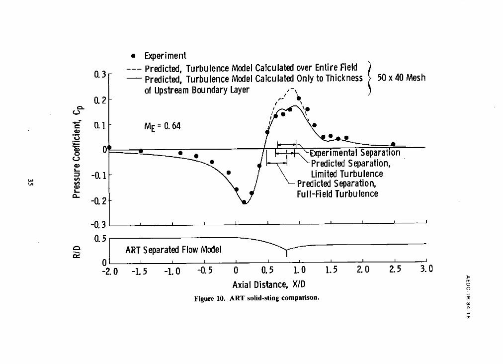
3.6 TURBULENCE MODEL VERIFICATION

Numerical experiments were performed for the configuration shown in Fig. 10 to

evaluate the two-layer model in separated flow. This configuration of an afterbody and solid

plume simulator was tested in the Acoustic Research Tunnel (ART) at AEDC, Ref. 20. As

shown in Fig. 10, the pressure distribution and the separation point prediction were

improved significantly if it were assumed that the boundary layer, after separation, became

essentially free of turbulent stress. A similar observation was made by Swanson, Ref. 21,

relative to solutions of the Navier-Stokes equations about a configuration very similar to the

ART model. He found that a relaxation turbulence model suggested by Shang and Hankey,

20

AEDC-TR-84-18

Ref. 22, improved his results significantly. According to Swanson, this was because tl~e eddy

viscosity was decreased in the outer (separated) layer, which served to decrease the plateau

pressure, bringing it into better agreement with measurements. Good results were obtained

with the ART model by restricting the turbulent viscosity to the region near the body no

larger than the attached, upstream, in-flow boundary-layer thickness. As a practical matter,

this was accomplished by terminating the calculation of turbulent viscosity at the grid point

away from the body surface nearest the thickness of the boundary layer. A family of

pressure distribution curves between the upper and lower curves of Fig. 10 may be calculated

by varying the point of termination of turbulence from the thickness of the boundary layer

to the width of the entire field. No calculations were made with the turbulence turned off

any closer to the body than the boundary-layer thickness. Because of these findings, the

turbulence was calculated only out to the thickness of the upstream boundary layer in the

comparisons with the FFA measurements that follow.

Since these numerical experiments with the Baldwin-Lomax model were conducted, a

new model has been introduced by Johnson and King, Ref. 16, that promises to overcome

the above difficulties. The model predicts more accurately the apparent viscosity in the outer

region of the separating boundary layer and, according to the paper, gives excellent

predictions of the pressure distribution in the separated region.

3.7 COMPUTED RESULTS AND COMPARISONS WITH MEASURED DATA

The method was applied to a configuration run by Agrell and White, Ref. 14, as shown

in Fig. 11, where the unit Reynolds number is 195,000/RN, RN is 15 mm, and the afterbody

boundary-layer shape is the I/7 power-law profile.

The configuration with a boattail of 8 deg was chosen because it ~,,as the one for which

the most results were shown in Ref. 14. The initial conditions used were free stream

everywhere with the upstream boundary-layer profile and thickness assumed along the entire

body-conforming coordinate. The nozzle exit conditions were set to the correct Mach

number for a conical flow nozzle, but the exit static pressure was initially set equal to the

ambient pressure. After approximaely 300 time steps, the nozzle exit pressure was increased

in stages up to the static jet-to-free-stream pressure ratio of interest. The maximum pressure

ratio of the experiments was 15.2. No upper limit to pressure ratio was determined; however,

the higher pressure ratios were more difficult to obtain because smaller time steps had Io be

used to assure convergence. Achieving a higher pressure ratio using a converged sohmon as a

starting point was usually more difficult than beginning from the initial conditions and

stepping the pressure every few hundred time steps.

21

AEDC-TR-84-18

The results and comparisons are presented in Figs. 11-20. The predicted point of

separation on the afterbody is compared with the measured results in Fig. 11. The

comparison is very good at the lower pressure ratios with a gradual underprediction

noticeable as the pressure ratio passes through twelve. This underprediction is attributed to

the decrease in grid resolution on the plume boundary at the reattachment point, because an

increase in the pressure ratio lifts the plume boundary out of the finer mesh region. This

situation could be helped by using an adaptive grid.

Also in Fig. I 1 is the separation curve computed using the Chapman-Korst component

method as described previously and shown in Fig. 6. It shows poor agreement for the lower

pressures. This is caused by the method's reliance on theory developed for free-interaction

separation before a forward facing step. This theory does not account for the effect of the

afterbody shape w, ith bluff base on separation. Thus when the separation becomes quite

large, the base effects being propagated upstream are diminished and agreement improves.

The Chapman-Korst component method is used at the AEDC as a quick screening method

to detemine whether separation could be a problem.

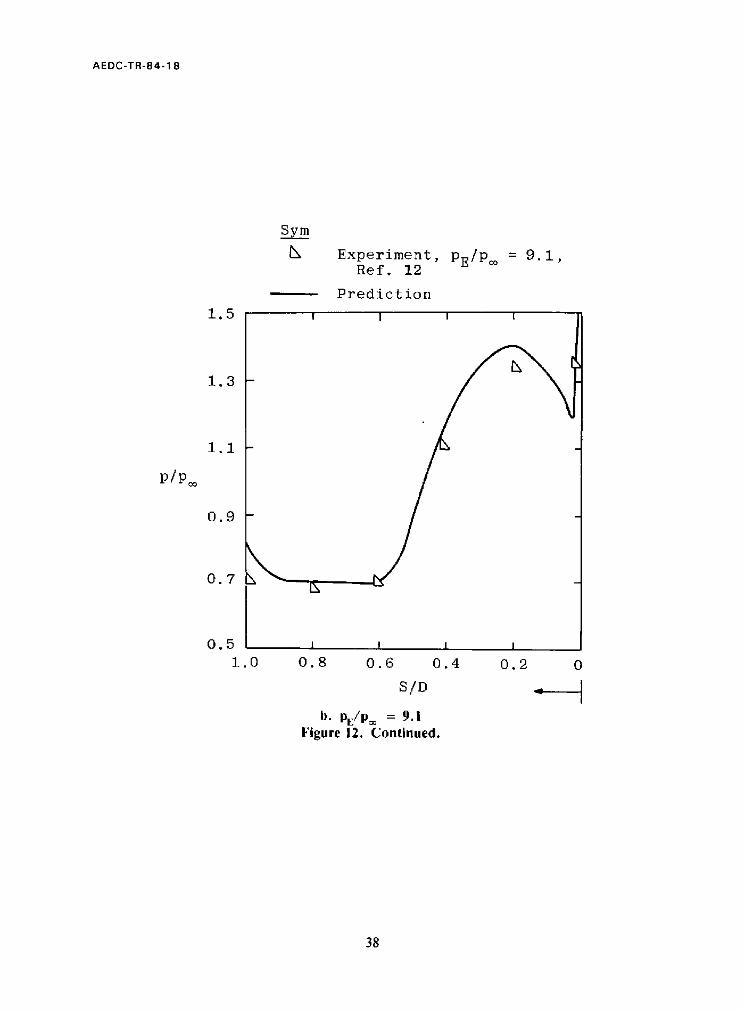
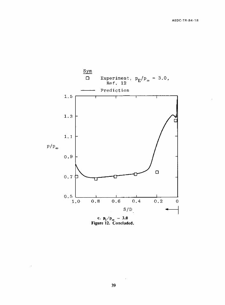
Figure 12 presents the comparison with experiment of the afterbody pressure

distribution. The predicted pressure distribution shows good agreement, except for the

plateau region. However, if the first peak is compared with the experimental plateau

pressures as in Fig. 13, the agreement is good. The dip in the pressure curve after the first

peak appears to be attributable to the lack of grid resoluuon and to the radius inserted in the

base/afterbody juncture.

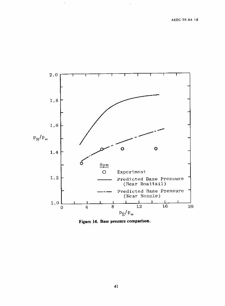
The base pressure shows poor agreement with measured data as shown in Fig. 14. The

base pressure has a fairly large variation on the bluff face. This is caused both by the base

corner radius and by the displaced boundary at the nozzle lip. No experimentation was

performed to determine the smallest radius allowable by the method. It is apparent from

calculations made on different configurations that this radius is much too large for the base

size. This size has caused the recirculating eddies to be displaced, causing, in turn, the

pressure disparity. Calculations made with different configurations also show that if

sufficient flat base area is maintained relative to the corner radius and the displaced

boundary, a typical flat pressure distribution on the face is obtained. Experimentation with

the position of the intersection of the displaced boundary and the base area showed that

moving the point changed the local base pressure, but not the position of separation.

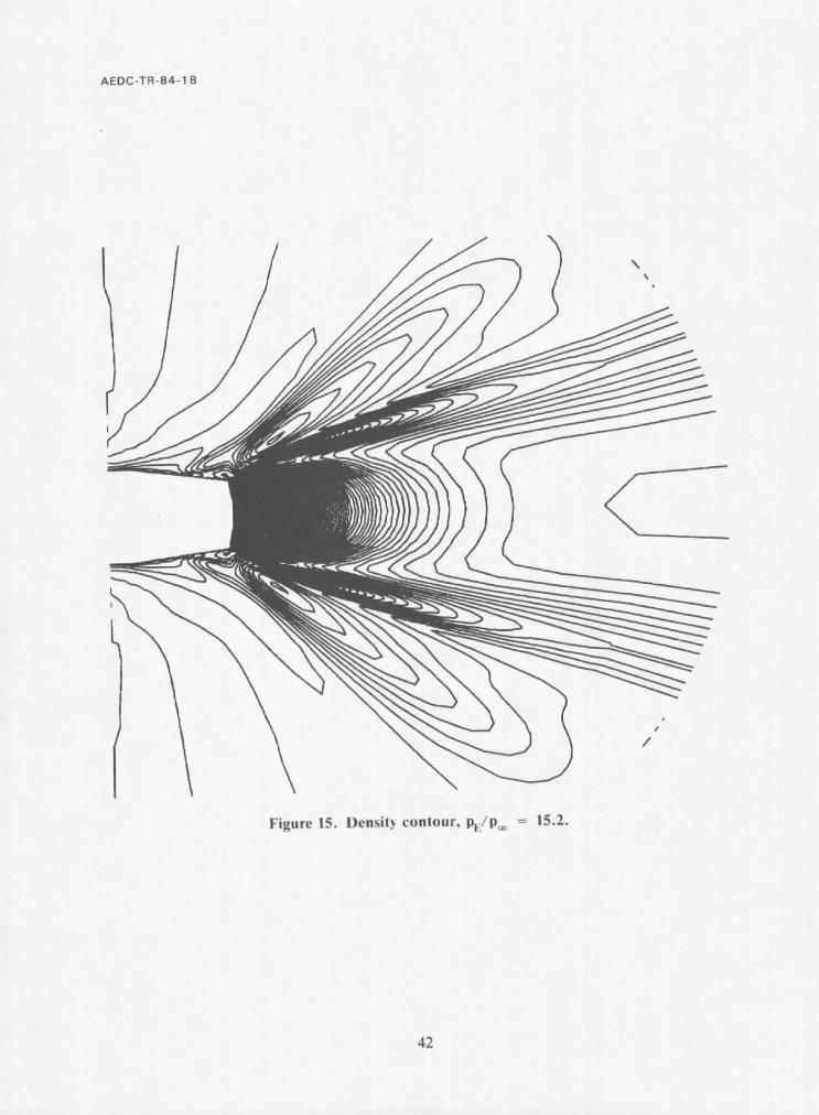
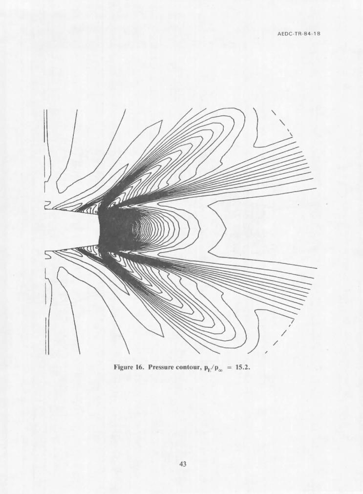
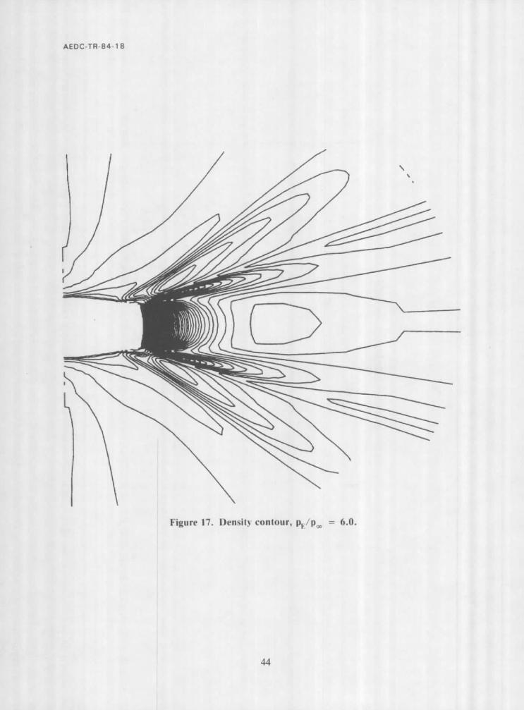
The contour plots of density and static pressure in Figs. 15 - 18 show the computed

features of the entire field. The lambda shock structure is readily apparent, and it is

particularly sharply defmed in the pressure contour plot at a pressure ratio of six. As the

22

AEDC-TR-84-18

pressure ratio is changed from six to 15.2, the separation localion, as indncated by Ihe

separation shock, moves upstream. The trailing shock structure, however, is not well-

resolved.

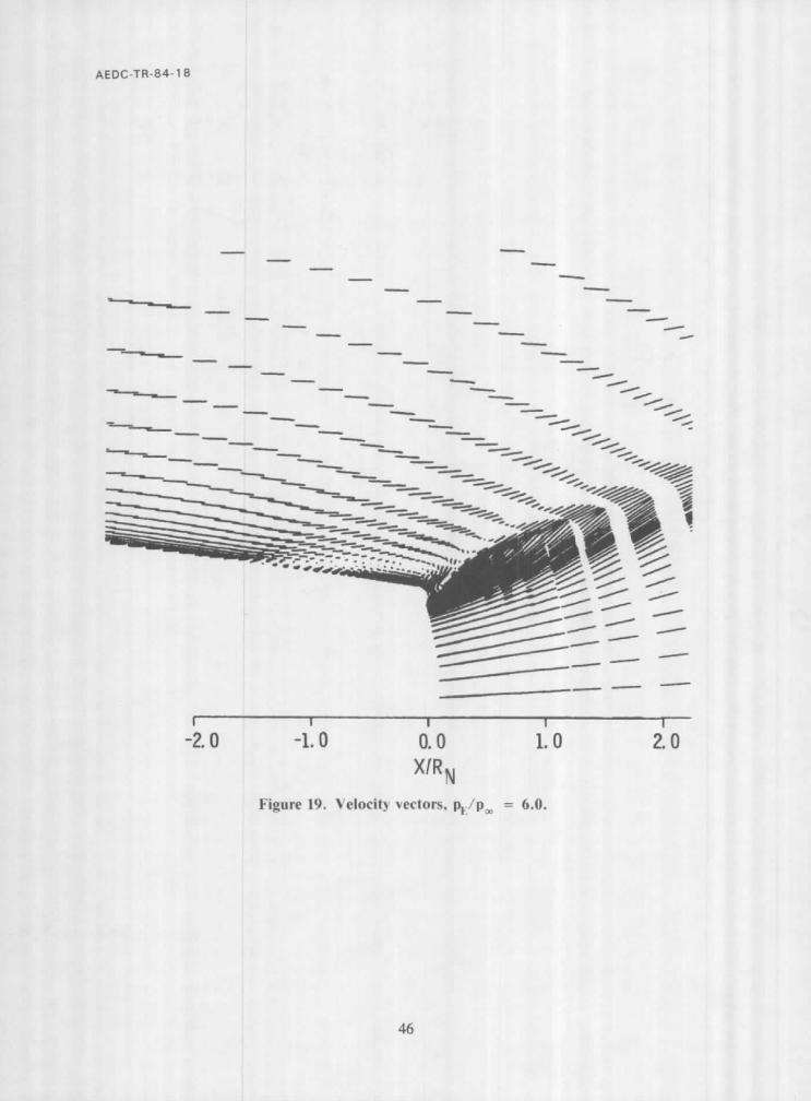
Figures 19 and 20 show further the amount of information provided by the method.

They are plots of velocity vectors. Separated areas are easily identified by the abrupt change

in velocity on the afterbody.

Converged predictions of separation location were achieved in approximately 2,100 sec

of CRAY-1S processing time for each case presented. Significant changes in separation

location cease after about 1,800 sec.

In summary, a thin-layer, implicit Navier-Stokes method was used to solve the plume-

induced separation problem. To achieve high static jet-to-free-stream pressure ratios, the

nozzle lip was removed from the region of the viscous solution and solved inviscidly as a

centered expansion. The predictions were very good, except at the highest pressure ratios,

where underprediction of separation apparently resulted from poor grid resolution, it was

also demonstrated that the thin-layer approximation is legitimate for calculating large

separated flow regions if care is taken with the turbulence model, and that the nea[ wake

could be treated adequately if considered as being largely devoid of viscous effects. The

method demonstrated a marked improvement in accuracy over the Chapman-Kor~t

component method, achieving a predictive accuracy sufficient to allow the method to be

used as an engineering tool. Also, it permits solutions of plume interference problems in the

flow regimes where the Chapman-Korst component method fails. The accuracy of this

approach is expected to improve with improved grid resolution when larger computer

memory becomes available.

4.0 CONCLUSIONS AND RECOMMENDATIONS

Two methods for determining the extent of plume-induced separation on afterbodics in

supersonic flow have been developed. The first, a Chapman-Korst component method that

uses an external separation criterion, produces quite good predictions at very high jet-to-

free-stream pressure ratios where extensive separation is present. It does not predict small

separation regions well, and it fails when the trailing shock system has embedded subsonic

flow. However, because of its speed and relative ease of use, coupled with the fact that it wdl

predict the type of separation that could blank a control surlace, it is the first choice for

quick screening of possible effects of chamber pressure and afterbody design.

The second method presented requires the solution of the thin-layer Navner-Stokcs

equations. This method shows its strength in these very flow regimes where the component

23

AEDC-TR-84-18

method fails, i.e., regimes where the extent of separation is relatively small and regimes

where extensive subsonic flow occurs. The thin-layer form of the equations proved to be

more accurate than the component method at low to moderate pressure ratios. Hov,,ever, at

higher pressure ratios, convergence becomes more difficult and careful attention to the grid

structure is required. Still, where the component method is a mature technology, the Navier-

Stokes method shows potential for further refinement to the point where it may be used

routinely for highly accurate predictions of separated flows.

Resources should be turned now to the development of better Navier-Stokes methods.

This will require the implementation of better turbulence models, more computer memory,

and, of course, higher computational speeds. Refinement of algorithms is also required so

that the nozzle-lip problem may be handled without resort to artifices such as described in the text.

R E F E R E N C E S

I. Chang, P. K. Separation of Flow. Pergamon Press, New York (First Edition). 1970.

. Bauer, R. C. and Fox, J. H. "An Application of the Chapman-Korst Theory to

Supersonic Nozzle-Afterbody Flows." AEDC-TR-76-158 (AD-A035254), January 1977.

3. FOX, J. H. "A Generalized Base-Flow Analysis with Initial Boundary-Layer and

Chemistry Effects." AEDC-TR-79-46 (AD-A072683), July 1979.

. Fox, J. H. and Bauer, R. C. "Analytical Prediction of the Base Pressure Resulting

from Hot, Axisymmetric Jet Interaction in Supersonic Flow." AIAA Paper 81-1898,

AIAA Atmospheric Flight Mechanics Conference, Albuquerque, New IVlexico, August 1981.

. Chapman, A. J. and Korst, H. H. "Free Jet Boundary with Consideration of Initial

Boundary Layer." Proceedmgs of the Second U. S. National Congress of Applied Mechanics, The American Society of Mechanical Engineers, New York, 1954, pp. 723-731.

. Korst, H. H., Chow, W. L., and Zumwalt, G. W. "Research on Transonic and

Supersonic Flow of a Real Fluid at Abrupt Increases in Cross Section - - Final

Report." ME Technical Report 392-5, University of Ilhnois, Urbana, December 1959.

24

AEDC-TR-84-18

. Hahn, M., Rubbert, P. E., and Mahal, Avtar S. "Evaluauon of Separation Crilcrm

and Their Application to Separated Flow Analysis." AFFDL-TR-72-145, January

1973.

8. Bauer, R. C. "An Analysis of Two-Dimensional Laminar and Turbulent Compressible

Mixing, AIAA Journal, Vol. 4, No. 3, March 1966, pp. 392-395.

9. Strickland, J. H., Simpson, R. L., and Barr, P. W. "Features ot a Separating Turbulent Boundary Layer in the Vicinity of Separation." Journal of Flutd Mechanics.

Vol. 79, Part 3, March 1977, pp. 553-594.

10. Strickland, J. H. and Simpson, R. L. "The Separating Turbulent Boundary La},cr: An Experimental Study of an Airfoil Type Flow." Technical Report WT-2, Southern

Methodist University Thermal and Fluid Sciences Center, August 1973.

I 1. Petri, Fred. "The Addition of Secondary Shock Capability and Modifications to the GASL Three-Dimensional Characteristics Program. Part I: Analysis and Results". General Applied Sciences Laboratory Report TR-653, (AD659808), August 1967.

12. Whitfield, D. L. "Integral Solution of Compressible Turbulent Boundary Layers Using Improved Velocity Profiles." AEDC-TR-78-42 (AD-A062946), December 1978.

13. James, C. R., Jr. "Aerodynamics of Rocket Plume Interactions at Supersomc Speeds." AIAA Paper No. 81-1905, AIAA Atmospheric Flight Mechanics Conference,

Albuquerque, New Mexico, August 1981.

14. Agrell, J. and White, R. A. "An Experimental Investigalion o1" Sup ersontc

Axisymmetric Flow over Boattails Containing a Centered Propulsive .let." FAA

Technical Note AU-93, 1974.

15. Baldwin, B. and Lomax, H. "Thin-Layer Approximation and Algebraic Model for Separated Turbulent Flows." AIAA Paper 78-257, AIAA 16th Aerospace Sciences

Meeting, Huntsville, Alabama, January 1978.

16. Johnson, D. A. and King, L. S. "A New Turbulence Closure Model tor Boundary

Layer Flows with Strong Adverse Pressure Gradients and Separation." AIAA Paper

84-0175, AIAA 22nd Aerospace Sciences Meeting, Reno, Nevada, 1984.

25

AEDC-TR-84-18

17. Deiwert, G. S. "A Computational Investigation of Supersonic Axisymmetric Flow

over Boattails Containing a Centered Propulsive Jet ." AIAA Paper No. 83-0462,

AIAA 21st Aerospace Sciences Meeting, Reno, Nevada, January 1983.

18. Pulliam, T. H. and Steger, J. L. "Implicit Finite-Difference Simulations of Three-

Dimensional Compressible Flow." A I A A Journal, Vol. 18, No. 2, February 1980, pp.

159-167.

19. Thomas, P. D. "Numerical Method for Predicting Flow Characteristics and Performance of Nonaxisymmetric Nozzles, Part 2 - - Applications." NASA

Contractor Report 3264, Langley Research Center, Virginia, October 1980.

20. Benek, J. A. "Separated and Nonseparated Turbulent Flows about A,dsymmetric

Nozzle Afterbodies, Part II, Detailed Flow Measurements." AEDC-TR-79-22 (AD-

A076458), October 1979.

21. Swanson, Charles R., Jr. "Numercial Solutions of the Navier-Stokes Equations for

Transonic Afterbody Flows." NASA Technical Paper 1784, Langley Research Center,

Virginia, December 1980.

22. Shang, J. S. and Hankey, W. L., Jr. "Numerical Solution for Supersonic Turbulent Flow over a Compression Ramp." AIAA Journal, Vol. 13, No. 10, October 1975, pp.

1368-1374.

23. Simmonds, James G. A Brief on Tensor Analysis. New York, Springer-Verlag, 1982.

26

AEDC-TR-84-18

/ ¢ Separated Layer--~ / ~

Separation S h o c k y ~ K ~__p 1 u m - - ~ \/ ~ ~ e

~ Barrel

Reattachment Shock

Boundary

Shock

Figure 1. Schematic of plume interaction.

Reat tachment Separation Shock---~ / / ,%¥~e, Shock

Separation Layer--~ S ~ _ ~ ~ "

Stream 2 ~ ~ ~ ~ J ~ ~ Point I ~-~ ~ k___ Plume ~oundary

" l l l l l l l l l l t / / J " - - - H i g h - S p e e d E d g e o f

c L - -

Figure 2. Interaction showing shear-layer model.

27

AEDC-TR-84-18

J YU'

Y m

YS

YL

(

~2

Point i \

J v / X

S

Ill

-Trailing Shock/

U

PB X 1

/ Figure 3. Details of recompression region.

28

AE

DC

-TR

-84

- 1

8

r-~

0 @

.~

I

@

0

O0

E

~b

~ ~-~

~0

0

I

I I

I I

I

<3

n(]

13

D

o')0

cg,~

II II

4

nn[]d~

I

0 00

b~

o ~;)

,_

0 ,-

@

c~

- ~ E

¢x]

Q~

L

0

I I

1 0

¢,') ~

] 1-1

0 I

29

AED

C-TR

-84-18

Z

I.. .-t IO II

d O O

r+.4

O

0 03

"-7 I I

4~ 0

"ci O

I-4

I:::; LO

O

t"..

# II

,~ 8

.rig

O..~

• b~ 0

-- "t~

"0

0 •

0 .e-I

O

0 0

/ LfD

CO

II 8

I d

O

0 uO

co

II 11

II ~-

8 8

8 ,--

D-,

~ D..,

~ ~7,

0

,d~ ,~

q~,

I O

d

O

O

u3

II 8

D~

L)

I u~

O

d

~'11 I

I I

.r-t

,-",1 ~ ~

rj

• ,..-i ~.

I O

u2. O

I

,6 O

o.~-- ~ E O E O O

,m

O

=

u3 "~

w

"O

I-

O I

~ '-"

ID

I

O

O

cxl O

I

O I

30

AE

DC

-TR

-84

-18

I

o.-,0,1

0 P

°P

I

,--I 0

0

-- I~

C

D-

,~

0 "~

0 I

~o~ m

I

~o

\ \ \ \ \ \ \ \ \ \ \

I,o

\ \ \ \ \

0

t~

II b~

00 hi:

q; ¢o

q; O

--

0 ~

Z a

0 in

0

0 C

O

o1 II

cq o,1

II II

Z II

II

1:1 ~

r q 8

\ \ \ \ \ \

I i

I I

0 ~

0 ~

~-4 ~

1

o o

o o

\ \

0

\ \

.% 0

,---t

'--" 0 0

0 ~

1

o

q O

0,1

0

I-

0 0 °m

l

t.

=1

31

AEDC-TR-84-18

Figure 7. Computational grid.

32

AEDC-TFI-84-18

~ . . . . ~ , , ~ - - A c t u a I Juncture

(r Radius_ Used i n ' " ~ /..---Base Computations-/ "~

Nozzle Lip with ~___/ Centered Expansion )

Nozzle Exit Plane J ' ~

Figure 8. Schematic of base region.

33

I

AEDC-TR-84-18

Nozzle Exit P l a n e ~ /

i f

f

i f

r-Grid for N-S Solver

/ /

/ / / /

/ /

/ / i / 7 i

f I I t I I

f / /

/ /

/

/

Method of Characteristics Grid

Figure 9. Overlapping grids.

34

AE

DC

-TR

-84

-18

Jl o

=o *

°

/1_~-_ m

"-

I= u

lie,)

s.. Q

.~ 0

~--

~,'~

- o

L

I-E

.-- .~w

-~ "~

E

0 ~

.} -I-,

.~

,., .,-.

_.7 /e-

,.-..__. ,-,

,, L.

>,

~ l~

a---~

'

.,_~ ~

('_ _

Li-t-f~

=

=

"-._-I.. ~r

~ -

"~

I_

---t- t~3

~-

E

m

m

D

I •

I I

I I

d d

d II

I

1

e,i

e4

/---

/

0 k_

i dl

i i

d d

c:~ c~

!

I !

d3 '},uapujao3 aJnssaJcl

o ~,

C]I~

,,,4 X

E

t,,#

t"

o~ m

@

• ~ [- ,..-

,,," ._=

35

AE

DC

-TR

-84

-18

O

O

01

oo

S 0 II

II Z

0

~D

II

d x

II II

~ N

ee

\ i___

, ,o \ \ \ \

\ k

IE ,--~

O~

~

O

O

r-H

O

O

r-t

O

O

\ o~

o \ \ ,

1o,

\ \ \

\ \ \ \

I I

I I

O0

t~D

~t ~ ¢xl

o o

o o

~O

O

O

• ,-~ O

O

• ,-I 4.~

O

• O

0~ E

I

O

0

0 0

0 ;.~. 0

,~.

d

%

O

¢q

O

OO

~t ~

¢q

O

O

E

Z O

L

O

O

om

:E

L--

36

A E D C - T R - 8 4 - 1 8

Sym

0 Experiment, Ref. 12

Prediction

pE/p ~ = 15.2,

1.5i 1 I I I

1 . 3 0

P/P~o

I.I

0.9

0

0.70

0.5 1.0

I I I

0.8 0.6 0.4

S/D

I I

0 . 2 0

---4 a. p~tp~ = 15.2

Figure 12. Afterbody pressure distribution.

37

AEDC-TR-84-18

P/Poo

1 .5

1 . 3

i.i

0.9

o.7

0 . 5 1 . 0

Svm

Experiment, pE/p ~ = 9.1, Ref. 12

Prediction

I I !

I I I

0.8 0.6 0.4

S/D

b. q/p= = 9.! Figure 12. Continued.

I

0.2 0

38

AEDC-TR-84 - 18

PlP~o

1.5

1.3

I.I

0.9

0.7

0.5 1.0

Sym

[] Experiment, pE/p~ = 3.0, Ref. 12

Prediction

I I I

1"3

I I I

0.8 0.6 0.4

S/D

c. ~:/p~ = 3.0

Figure 12. Concluded.

0.2 0

39

AEDC-TR-84-18

P/P~

1.6

1.4

1.2

1.0

71 by 30 by 5 Mesh

l I

[]

[] Sym

[]

[]

Experiment

Predrcted

I I I 4 8 12

PE/P,~

Figure 13. Plateau pressure comparison.

I 16 20

40

A E D C - T R - 8 4 - 1 8

PB/Poo

2.0 I I I I I I I I I

1 .8

1 .6

1 .4

1 .2

1 .0 0

J /

0 Sym

0 0

I I 4

Figure 14.

0 Experiment

Predicted Base Pressure (Near Boattail)

Predicted Base Pressure - (Near Nozzle)

I I I I I I 8 12 16 20

PE/P~

Base pressure comparison.

41

AEDC-TR-84-18

!

/

/

Figure 15. Densit~ contour, p w l p ~ = 15.2.

42

AEDC-TR-84-18

\

\ \

f

Figure 16. Pressure contour, pv:/p~ = 15.2.

/

/

43

AEDC-TR-84-18

\

Figure 17. Density contour, pl,:/p~ = 6.0.

44

AEDC-TR-84- 18

\

\

\

Figure 18. Pressure contour , P~:/Poo = 6.0.

/ /

/ #

45

AEDC-TR-84-18

m

m

m ~

!

s

w m

m ~ m

_ - . - . . _ . _ _ ~

-2. 0 -1.0

Figure 19.

~ . . _ _ . _ _ _ . . _ _ . l _ -----

I I

0.0 1.0 X/R N

Velocity vectors, pE/p= = 6.0.

I

2.0

46

AEDC-TR-84-18

m

m

m

!

. . . _ . - . - _ . ~

i I I I I

-2.0 -1.0 0.0 1.0 2.0 X/R N

Figure 20. Velocity vectors, pE/poo = 15.2.

47

AEDC-TR-84- I 8

APPENDIX A TRANSFORMATION TO CURVILINEAR COORDINATES

Consider the general form of the dimensionless conservation equations in Cartesian

coordinates.

0tq + OxE + 0yF + 0zG = R e - l ( 0 x R + OyS + OzT) (A-l)

where Ox - O/Ox,etc.

Define vectors such that

cq = [q, E, F, G] -- IV I, V 2, W 3, V 4]

XV = [ R , S , T ] - [ W ' , W 2 , W 3]

Equat ion (A-I) may now be written in divergence form as

V.V/ = 1 V . W (A-2) Re

From tensor analysis, viz. Ref. 23, in general coordinates

V • W = Jlgx, ( J - IV i )

and

V • W = J(gx~ ( J - lWl )

where the Jacobian notat ion, J, is inverted to conform with Pull iam and Steger. Elements V i

and W ~ are the contravariant components of V and "~. The divergence is invariant under

t ransformat ion as are the vectors; therefore, the only effort required is in determining these

vector components in the curvilinear system.

Contravariant vectors components t ransform from Cartesian [t,x,y,z] to curvilinear [r,

~, r/, g'] coordinates as

~t = (StrV 1

V2 = 0t~V I + 0x~V 2 + 0y~V 3 + 0z~V 4 (A-3)

49

AEDC-TR-84-18

V3 = 0t,r/V I + 0xr/V 2 + Oy,r/V 3 + 0z~,/V 4

V4 = Ot~-V 1 + 0xg-V 2 .{.. 0y~-V 3 + 0z~-V 4

m

In the s a m e way , W i - - W '

a l so

whe re ~x - 0 ~ , etc.

F r o m Eqs . (A-2) a n d (A-3)

whe re

J =

rt 0 0 0

~t ~x ~y ~z

r/t r/x r/y r/z

~t ~'x ¢'y ¢'z

(A-4)

D

q - j - I V l , E - j - l V2, F - j - l ~ Z 3 , a n d ~ _- J - I V 4

a n d m j - 1 ~/,1, S ~ j - I W2, T m j - I W 3

T h e f o r m o f the c o n s e r v a t i o n e q u a t i o n s tha t is usua l ly s h o w n is o b t a i n e d by subs t i tu t ing the

var iab les fo r the v e c t o r c o m p o n e n t s in to Eq . (A-4) .

F o r example , cons ide r the ~ m o m e n t u m e q u a t i o n . T h e C a r t e s i a n c o m p o n e n t s are

V I -- q - Qu, V 2 - E -- QU 2 + p, V 3 -- F --- QvO, V 4 -- G - 0 u w

W 1 -- R - rx×, W 2 - S - rxy, W 3 - T - rxz

T h e s e are subs t i t u t ed in to Eqs . (A-3) . T h e n Eqs . (A-3) are subs t i t u t ed in to Eq . (A-4) .

50

I AEDC-TR-84-18

The lef t -hand side o f Eq. (A-4) becomes

OJ-I Ou + OJ-] ~t Ou + OJ-I ~x(OU 2 + p)

Or O~ Or;

O J - I ~y (our) +

+ O J - I ~ (ouw) OJ - 17t Ou

+ 07

+ O J-1 7x(OU 2 + p)

07

OJ - t 7v(OUV) +

07

-1 nzt,~uw~,~. OJ + 07

+ OJ- l~ ' tOu I- OJ-l~ 'x(OU2 + p) OJ - I ~'y(QUV) +

Letting

+ = RHS Oz

U = ~ t + ~,u + ~ y v + ~zw

we get

U = 7/t + r/xU + r/yV + r/zW

W = ~'t + ~'xU + ~'yV + ~'zw

0 J - 1 o u + 0J-I(QuU + ~xP) + 6qJ-l(o uV + 7xP) + 0 J - l ( 0 u w + ~'xP)

Or O~ On O~ = RHS

and

RHS = Re- I O~J-I (~x rxx + ~yrxy + ~zrxz) + 0,J-l(~7,r~x + r/yr,~ + r/zr, z)

+ 0~.J-l(~'xrxx + ~'yT"xy + ~'zT'xz)

or for the thin-layer approximat ion:

RHS = Re-1O~-J-l(~'xrx~ + ~'yrxy + ~'zrxz)

The other conservat ion equat ions I~ransform as easily.

51

AEDC-TR-84-18

a

Cp

Cp

C

H

L

eeff

~vir

M

n

P

Pr

R

Reu

U

U

NOMENCLATURE

Sound speed

Static pressure coefficient

Specific heat at constant pressure

Total energy

Total enthalpy

Effective thermal conductivity, k = cp (ttM/Pr + /xt/0.9)

Body length

Length of mixing region; mixing length in turbulence model

Effective mixing length

Virtual mixing length

Mach number

Inverse of power-law exponent

Static pressure

Prandtl number

Radius from axis of symmetry

Average radius

Unit Reynolds number

Velocity of high-speed edge of shear layer in direction of shear layer

Velocity component in Cartesian x direction; velocity in direction of development shear layer

52

U , V , W

V, W

X

X

Y

lr'/p

#

~t

P-M

AEDC-TR-84-18

Contravariant velocity components

Velocity component in Cartesian y and z directions, respectively

Coordinate along slipline in recompression region

Cartesian axial coordinate or mixing coordinate in direction of developing

mixing layer

Cartesian coordinate transverse to x coordinate

Angle between slipline and mixing layer, Fig. 3; also used for nozzle and

afterbody angles

Boundary-layer thickness

Ratio of specific heats

Curvilinear coordinate approximately normal to body, also boundary-layer

coordinate, y/6

Dimensionless mixing variable; body-conforming curvilinear coordinate in

azimuthal direction

Dimensionless position parameter, o6/t

Velocity ratio in shear layer, u/U

Shear stress; time

Effective viscosity: molecular + turbulent, except when subscripted

Turbulent viscosity

Molecular viscosity

Body-conforming curvilinear coordinate in flow direction

Density

53

AEDC-TR-84-18

o Mixing or spreading parameter

ao Incompressible a, a reference value

oo Vorticity

SUBSCRIPTS

B

D

E

O0

L

M

m

N

S1

$2

T

U

Beginning of recompression; also upstream of shock wave

End of recompression; also downstream of separating shock wave

Separated region; base region

Dividing streamline

Nozzle exit condition

Free-stream condition

Low-speed edge of mixing layer

Molecular

Inviscid boundary with respect to origin of mixing profile

Nozzle

Downstream of recompression shock wave

Stagnating streamline

Stream 1 (jet plume)

Stream 2 (outer stream)

Total condition

High-speed edge of mixing layer

54