Two Aspects of Topology in

Graph Configuration Spaces

Molly Elizabeth Ison

Thesis submitted to the faculty of

the Virginia Polytechnic Institute and State University

in partial fulfillment of the requirements for the degree of

Master of Science

In

Mathematics

Professor Peter Haskell, Chair

Professor Ezra Brown

Professor Daniel Farkas

7 October 2005

Blacksburg, Virginia

keywords: braid group, manifold, pseudomanifold with boundary, fundamentalgroup, graph, configuration space

Abstract

Two Aspects of Topology in

Graph Configuration Spaces

Molly Ison Gardner

Virginia Polytechnic Institute and State University

Professor Peter Haskell, chair

A graph configuration space is generated by the movement of a finite numberof robots on a graph. These configuration spaces of points in a graph are topo-logically interesting objects. By using local, combinatorial properties, we definea new classification of graphs whose configuration spaces are pseudomanifoldswith boundary. In algebraic topology, graph configuration spaces are closelyrelated to classical braid groups, which can be described as fundamental groupsof configuration spaces of points in the plane. We examine this relationshipby finding a presentation for the fundamental group of one graph configurationspace.

Acknowledgements

This paper would not have been possible without my advisor, Dr. Peter Haskell.He helped and encouraged me through every step.

I am also grateful to my husband, R. Matthew Gardner, for his love andsupport.

iii

Contents

1 Introduction . . . . . . . . . . . . . . . . . . . . . . . . . . . . . . 12 Background and Examples . . . . . . . . . . . . . . . . . . . . . . 2

2.1 Robotics . . . . . . . . . . . . . . . . . . . . . . . . . . . . 22.2 Braid Groups . . . . . . . . . . . . . . . . . . . . . . . . . 32.3 Definitions and Notation . . . . . . . . . . . . . . . . . . . 32.4 Configuration Spaces: 2-manifolds and 2-pseudomanifolds

Without Boundary . . . . . . . . . . . . . . . . . . . . . . 53 Configuration Spaces: 2-pseudomanifolds With Boundary . . . . 8

3.1 Preliminaries . . . . . . . . . . . . . . . . . . . . . . . . . 83.2 Cyclic Graphs . . . . . . . . . . . . . . . . . . . . . . . . . 103.3 Graphs on Six Vertices . . . . . . . . . . . . . . . . . . . . 133.4 Graphs on Five Vertices . . . . . . . . . . . . . . . . . . . 183.5 Graphs on Four Vertices . . . . . . . . . . . . . . . . . . . 19

4 The Fundamental Group of a Configuration Space . . . . . . . . 234.1 Fibrations . . . . . . . . . . . . . . . . . . . . . . . . . . . 234.2 Algebraic Topology . . . . . . . . . . . . . . . . . . . . . . 244.3 Homotopy Equivalence . . . . . . . . . . . . . . . . . . . . 264.4 Application of the Seifert-Van Kampen Theorem . . . . . 314.5 Presentation of the Fundamental Group . . . . . . . . . . 36

5 Appendix of Figures . . . . . . . . . . . . . . . . . . . . . . . . . 40

iv

1 Introduction

What are graph configuration spaces and why are we interested in studyingthem? A configuration space is the space arising from finite generators taking allpossible positions that they may lawfully attain. For example, the configurationspace of a single robot moving freely in ordinary Euclidean space is simply R

3.In a graph configuration space, the movement of a finite number of robots islimited to the edges and vertices of a graph.

If graph configuration spaces were strictly mathematical, any number ofrobots might be on any given edge or vertex simultaneously. However, configu-ration spaces have practical applications in robotics, where a number of robotsmove along a network of rails. In a practical setting, it is necessary for theserobots to avoid collisions with one another. Constraints must be set in place toprevent collisions.

One interesting aspect of these configuration spaces is their topological struc-ture. Some configuration spaces are manifolds and some can be embedded inmanifolds. In [1], Aaron Abrams lays a foundation for the theory behind graphconfiguration spaces as well as classifying which graphs give rise to 2-manifoldsbased upon the movement of two robots. Praphat Fernandes furthers this workin [2] by classifying the two-robot systems which give rise to 2-pseudomanifoldswithout boundary.

Another aspect of graph configuration spaces is their relationship to classicalbraid groups, which can be described as fundamental groups of configurationspaces of points in the plane. Graph configuration spaces are specialized con-figuration spaces of points contained within a graph.

In the following chapters, the previous work done by Abrams and Fernandesin graph classification will be continued and expanded. Furthermore, we willfind a presentation of the fundamental group of one graph configuration space.

In Chapter 2, we will examine the two main motivations for our interest ingraph configuration spaces, robotics and braid groups. The constraints upon ro-botic movement on a graph will be further described, as well as the cell structurecomposing the configuration space. Previous work with manifold and pseudo-manifold spaces will be outlined along with a more complete definition of thesestructures.

Chapter 3 is composed of original work and will classify which graphs giverise to a specific type of space, namely the 2-pseudomanifold with boundary.This work uses local, combinatorial principles to view the cell structure of theconfiguration space.

In Chapter 4, we take a closer look at the relationship between the graphconfiguration spaces and the classical braid groups. The techniques in algebraictopology and homotopy are described which will obtain a presentation of thefundamental group of the configuration space for the graph K5, the completegraph on five vertices.

1

2 Background and Examples

This chapter includes an overview of the two main motivations for this work withgraph configuration spaces, robotics and braid groups. It was mentioned brieflyin the introduction that constraints must be set in order to avoid collisionsbetween robots on a graph. These will be defined along with the notation forthe cell structure of a configuration space. Lastly, we will consider the previouswork done by Abrams and Fernandes in classifying graphs whose configurationspaces are either 2-manifolds or 2-pseudomanifolds without boundary.

2.1 Robotics

Imagine a number of robots moving mechanically along set paths on a factoryfloor. The movement of these robots, limited to the edges and vertices of a graphbut otherwise freely moving, generates a graph configuration space. Some verycommon robots, called Automated Guided Vehicles (AGVs), are used to trans-port objects around a factory floor. AGVs are expensive and not designed totolerate multiple collisions. However, if these robots are on a physical plane withno restrictions on their movement, collisions will be inevitable. Obviously someconstraints are necessary in order to prevent the robots from being damaged.

There are a few ways that robots could be programmed to avoid collisions.If two robots were not constrained to a graph, it would be possible to designthem such that one robot could sense the other and move around it if collisionseemed imminent, making each collision avoidance a local phenomenon. Theserobots take a large amount of computing power and are therefore quite costly.Robots that are restricted to a graph of fixed paths are more practical and lessexpensive. “The resolution of a collision on a graph is a non-local phenomenon”[3], because at least one robot must make a change in its path before reachinganother robot. Once a graph of paths has been determined, it is desirable toarrange each robot to start at a specific, predetermined location while a vectorfield controls its movement around the graph so that collisions are impossible.Ghrist, Koditschek and Rimon explain the theory and some solutions to thisproblem in [4] and [5].

In order to generate a graph configuration space from robotic movement withno collisions, we would like to create constraints so that every robot is at leastsome fixed distance from every other robot. The natural structure of a graphsuggests the solution that every robot be at least one full edge apart at all times.When every robot is constrained in this way on a graph, the resulting generatedspace is a discretized configuration space. This discretized configuration spacewill be the type of graph configuration space used in the remainder of this paper.

To examine more throughly the applications of graph configuration spacesarising from robotics, see [3] or [6].

2

2.2 Braid Groups

The classical braid groups, which began as a way of studying knots, are an areaof mathematics with applications in topology, group theory and mathematicalphysics. A braid group can be described as the fundamental group of a config-uration space of points in the plane. The configuration space from which thebraid group is derived is generated by a discrete number of particles movingin R

2 without collisions. As particles move in time, represented by height inR

3, the particles’ paths cross over and under one another, forming the “braid”pattern.

Some immediate comparisons can be made between a braid group configura-tion space and a discretized graph configuration space. The graph configurationspace is also a configuration space of points, but its generators may only moveupon points within the graph. Unlike the discretized graph configuration spacewhich must remain at least one edge apart, the particles of the braid groupconfiguration space are parameterized such that no two particles may occupythe same point in R

2. Perhaps the largest difference between the two is thatbraid group configuration spaces are entirely dependent upon the number ofgenerators employed. Because the generators are completely free to move any-where within R

2, every braid group configuration space with seven generatorsis isomorphic to any other braid group configuration space with seven gener-ators. However, the discretized graph configuration spaces are dependent notonly upon the number of generators employed, but also upon the structure ofthe graph. The discretized configuration space generated by three robots mov-ing upon C7, the cyclic graph on seven vertices, is a very different space thanthat generated by three robots moving upon K7, the complete graph on sevenvertices.

For more information on braid groups and graph braid groups, that is, thefundamental groups of configuration spaces of graphs, see [7].

2.3 Definitions and Notation

The following graph-related definitions have been taken from [1] and [8].A graph is a triple consisting of a vertex set, an edge set, and a relation that

associates with each edge two vertices called its endpoints. Another definitionof a graph is as a 1-dimensional CW-complex. The 0-cells are vertices and the1-cells are edges. The shortest path metric mskes the vertex set of a grapha metric space, whose distances are denoted by d. The distance between twovertices, d(v1, v2) is the number of full edges on the shortest path between thetwo. Although the “distance” between two edges or a vertex and an edge cannot be defined precisely under the metric, the distance between two objectscan still be defined as the number of full edges on the shortest path betweenthe two. Two edges with a common endpoint, E1 and E2, or an edge E1 andits endpoint v1 would then have distances d(E1, E2) = 0 and d(E1, v1) = 0,violating the definition of a metric space. Although this shortest path distanceis not a true metric, we will use it as our distance measurement.

3

A loop is an edge whose endpoints are equal. We will use only looplessgraphs in our classification of graphs generating configuration spaces. Multipleedges are edges having the same pair of endpoints. A graph is simple if it hasno multiple edges. The degree of a vertex is the number of edges of which it isan endpoint. Adjacent vertices are endpoints of a common edge.

A path is a simple graph whose vertices can be listed so that vertices areadjacent if and only if they are consecutive in the list. A connected graph isone having a u, v-path for every pair of vertices u, v. A cycle is a simple graphwhose vertices can be placed on a circle so that vertices are adjacent if and onlyif they appear consecutively on the circle. A tree is a connected graph with nocycles. The complete graph Kn has n vertices and

(n2

)edges, one connecting

each pair of vertices. The complete bipartite graph Km,n has m + n verticesx1, ..., xm, y1, ..., yn and mn edges, one connecting xi to yj for each i and j.

Previously, we described the constraints upon robotic movement so thatevery robot must be at least one full edge apart from all other robots at all times.Now that we have our distance metric, we can define this parameterization forrobots R1 and R2 so that d(R1, R2) ≥ 1.

Definition 2.1. [2] Let R1, ..., Rn be a finite set of robots on a graph Γ. Ifsome robot Ri is on a vertex vi of Γ then let xi = vi. If Ri is on an edge Ei

then let xi = Ei. The discretized configuration space Dn(Γ) is the subset of allconfigurations of robots R1, ..., Rn such that d(xi, xj) ≥ 1 for all i, j with i 6= j.

Note that the labeling of the robots is not trivial. The configuration of tworobots where R1 is on vertex v1 and R2 is on vertex v2 is different than theconfiguration where R1 is on v2 and R2 on v1.

For the remainder of this paper, when we refer to the configuration space,unless otherwise specified, we are speaking of the discretized graph configurationspace.

The discretized configuration space is a cell complex. For any number ofrobots, a 0-cell is generated when each robot is positioned on a distinct ver-tex. Earlier classification has been done on configuration spaces generated bythe movement of two robots on a graph. In the cell complex composing suchconfiguration spaces, the 0-cells are generated by the stationary positions oftwo robots on two distinct vertices v1 and v2. The 1-cells are generated by onestationary robot on a vertex v and one robot moving along an edge E suchthat d(v,E) ≥ 1. The 2-cells are generated by two robots R1 and R2 movingalong two distinct edges E1 and E2 such that d(E1, E2) ≥ 1. A cell is labeledby its generating vertices and/or edges, so that the cells just described wouldbe labeled as 0-cell (v1, v2), 1-cell (v,E), and 2-cell (E1, E2). The tuples areordered so that the first entry is the position of the R1 and the second entryis the position of R2. In a cell complex generated by n robots, cells would belabeled by the n-tuple (p1, p2, ..., pn), denoting the ordered positions of robots1 through n.

Before moving on to more complex spaces, we will demonstrate the genera-tion of a simple graph configuration space.

4

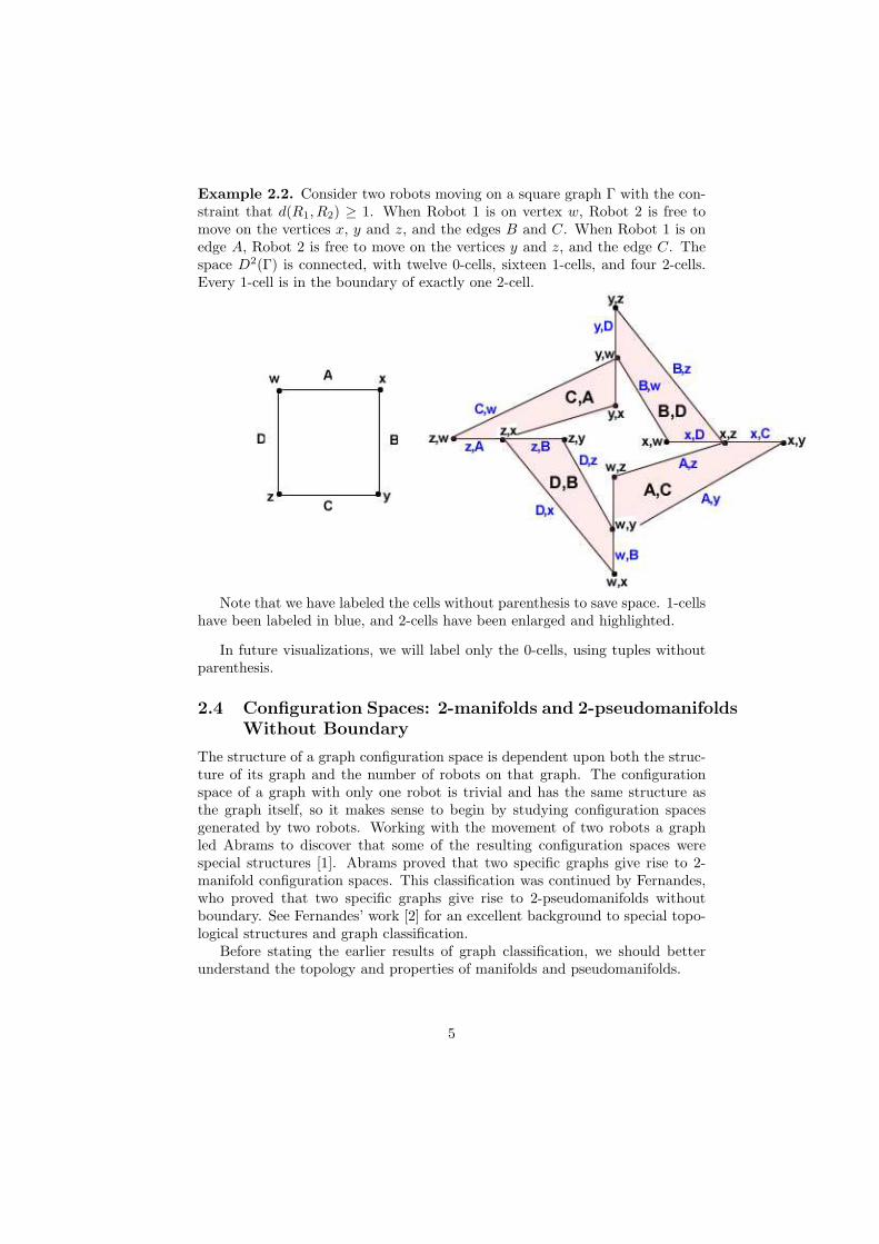
Example 2.2. Consider two robots moving on a square graph Γ with the con-straint that d(R1, R2) ≥ 1. When Robot 1 is on vertex w, Robot 2 is free tomove on the vertices x, y and z, and the edges B and C. When Robot 1 is onedge A, Robot 2 is free to move on the vertices y and z, and the edge C. Thespace D2(Γ) is connected, with twelve 0-cells, sixteen 1-cells, and four 2-cells.Every 1-cell is in the boundary of exactly one 2-cell.

Note that we have labeled the cells without parenthesis to save space. 1-cellshave been labeled in blue, and 2-cells have been enlarged and highlighted.

In future visualizations, we will label only the 0-cells, using tuples withoutparenthesis.

2.4 Configuration Spaces: 2-manifolds and 2-pseudomanifolds

Without Boundary

The structure of a graph configuration space is dependent upon both the struc-ture of its graph and the number of robots on that graph. The configurationspace of a graph with only one robot is trivial and has the same structure asthe graph itself, so it makes sense to begin by studying configuration spacesgenerated by two robots. Working with the movement of two robots a graphled Abrams to discover that some of the resulting configuration spaces werespecial structures [1]. Abrams proved that two specific graphs give rise to 2-manifold configuration spaces. This classification was continued by Fernandes,who proved that two specific graphs give rise to 2-pseudomanifolds withoutboundary. See Fernandes’ work [2] for an excellent background to special topo-logical structures and graph classification.

Before stating the earlier results of graph classification, we should betterunderstand the topology and properties of manifolds and pseudomanifolds.

5

Definition 2.3. The union of all k-dimensional and lower cells within a cellcomplex is called a k-cell complex. All cells of dimension lower than k arecontained in the closure of some k-cell.

Definition 2.4. The union of all (k-1)-cells that do not lie in the intersectionof at least two k-cells is called the boundary of a k-cell complex.

A 2-dimensional manifold, more commonly called the 2-manifold, is a 2-cellcomplex with the same local properties as the plane in Euclidean space. Aroundevery point of the 2-manifold, there is a neighborhood that is topologically thesame as the open unit ball in R

2. Using the properties of the cell structure,we define the 2-manifold to be a 2-cell complex in which every 1-cell lies in theintersection of exactly two 2-cells, permitting no singularities. A singularity ina graph configuration space would be a point in which the space was not locallyEuclidean.

One property of the 2-manifold that promoted earlier research was its ori-entability or nonorientability. It is speculated that a discretized graph configu-ration space is always orientable, but this remains an open question.

Definition 2.5. Let a path be started at any point of a manifold with a definitechoice of orientation and travel in that orientation around the surface of themanifold. If the path returns to its initial point with its original orientationreversed, the path is called orientation-reversing. If the path returns to itsinitial point with the same orientation with which it began, the path is calledorientation-preserving. A 2-manifold is called orientable if every closed path isorientation-preserving [9].

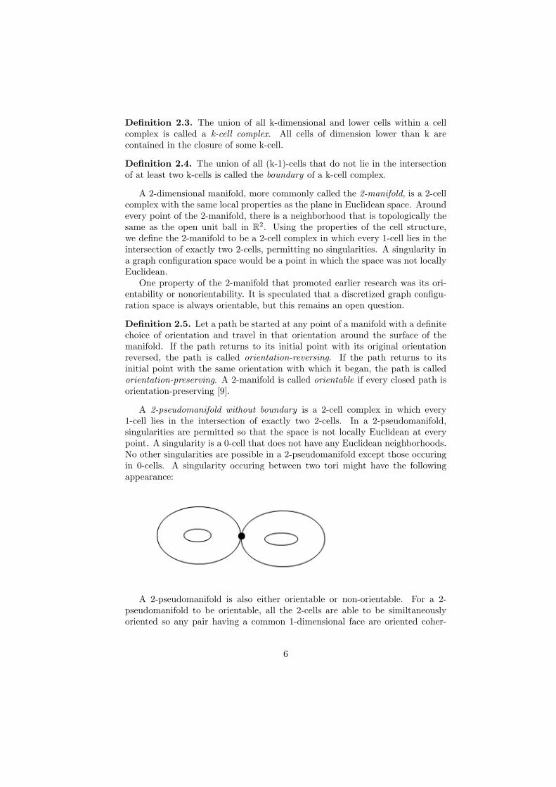
A 2-pseudomanifold without boundary is a 2-cell complex in which every1-cell lies in the intersection of exactly two 2-cells. In a 2-pseudomanifold,singularities are permitted so that the space is not locally Euclidean at everypoint. A singularity is a 0-cell that does not have any Euclidean neighborhoods.No other singularities are possible in a 2-pseudomanifold except those occuringin 0-cells. A singularity occuring between two tori might have the followingappearance:

A 2-pseudomanifold is also either orientable or non-orientable. For a 2-pseudomanifold to be orientable, all the 2-cells are able to be similtaneouslyoriented so any pair having a common 1-dimensional face are oriented coher-

6

ently. Pseudomanifolds are the most general structures that retain a meaningfulconcept of orientability. [9].

We now turn our attention to the specific graphs whose configuration spaceis a special structure. Each of these graphs has a configuration space generatedby two robots.

Theorem 2.6. [1] Let Γ be a connected graph without loops. If D2(Γ) is home-omorphic to a closed 2-dimensional manifold then Γ = K5, the complete graphon five vertices, or K3,3, the complete bipartite graph on six vertices.

Specifically, D2(K5) is homeomorphic to the 6-holed torus and D2(K3,3) ishomeomorphic to the 4-holed torus.

Theorem 2.7. [2] Let Γ be a connected graph without loops. If D2(Γ) is home-omorphic to a closed 2-dimensional pseudomanifold without boundary then Γ =doubled K4, the complete graph on four vertices with each edge doubled, or dou-bled C4, the cyclic graph on four vertices with each edge doubled.

The configuration space of the doubled C4 is composed of a cycle of fourtori, each joined to its neighbors by a single 0-cell. The configuration space ofthe doubled K4 is best described as a cube built out of six tori, in which eachtorus shares a single 0-cell with four distinct tori.

We observe that in each case, Γ was required to be both loopless and con-nected. Every graph for the remainder of this paper will be assumed looplessunless otherwise specified. We will briefly discuss connectivity in the next sec-tion.

7

3 Configuration Spaces: 2-pseudomanifolds With

Boundary

Now that we have defined 2-pseudomanifolds without boundary, we are readyto classify the graphs resulting in 2-pseudomanifolds with boundary. We recallthat the boundary of a 2-pseudomanifold is the union of all 1-cells that do not liein the intersection of at least two 2-cells. A 2-pseudomanifold with boundary isa 2-cell complex in which every 1-cell lies in the intersection of either one or two2-cells. A cell complex having a 1-cell that lies in the intersection of no 2-cells isnot a 2-pseudomanifold of any type, because singularities in 2-pseudomanifoldscan only occur in 0-cells.

This remainder of this section is composed of original work. Each of thefollowing graph configuration spaces is generated by two robots.

3.1 Preliminaries

There are some properties common to all graphs resulting in 2-pseudomanifolds,both with and without boundary. Perhaps the most intuitive is the necessity ofconnectivity. Consider two robots on a disconnected graph. If the robots areon the same component of the graph, the configuration space will be generatedonly by that single component. If the robots are on two different components Γ1

and Γ2, the configuration space will be Γ1 ×Γ2, and no interchange of positionswill be possible. Thus it is necessary for configuration space generating graphsto be connected.

The following theorems deal primarily with vertex degrees in Γ. Corollaries3.2 and 3.4 will be used repeatedly in later proofs to identify acceptable andunacceptable graph arrangements.

Theorem 3.1. If Γ is a connected graph with a 2-pseudomanifold configurationspace, with or without boundary, then every vertex in Γ is adjacent to at leasttwo other vertices.

Proof. Let Γ be a connected graph with a 2-pseudomanifold configuration space.By the definition of D2(Γ), Γ cannot be a single vertex. If Γ consisted of two con-nected vertices, then D2(Γ) would be a single 0-cell and not a 2-pseudomanifold.Thus Γ has at least three vertices.

Suppose that there exists some vertex v in Γ such that v is adjacent toexactly one other vertex w. Let {E1, ..., Em}, m ≥ 1, denote the set of edgeshaving both v and w as endpoints. Vertex w must be adjacent to at least oneother vertex x, lest Γ have only two vertices, so that w and x are endpoints ofat least one edge F . Now all edges with endpoint v are such that d(Ek, F ) < 1,1 ≤ k ≤ m. Therefore, the 1-cell (v, F ) in D2(Γ) is in the boundary of no 2-cellsand D2(Γ) is not a 2-pseudomanifold. Every vertex in Γ must be adjacent to atleast two other vertices.

8

Corollary 3.2. If Γ is a simple, connected graph with a 2-pseudomanifold con-figuration space, with or without boundary, then every vertex in Γ has degree atleast 2.

Theorem 3.3. If Γ is a connected graph with a 2-pseudomanifold configura-tion space, with or without boundary, then Γ contains no 3-cycle with a vertexadjacent to exactly two other vertices.

Proof. Let Γ be a connected graph with a two-pseudomanifold configurationspace. Assume that Γ contains a 3-cycle with vertices v, x and y, where vertexv is adjacent to only the two vertices x and y. Vertices x and y are the mutualendpoints of edge(s) [E1, ..., Em] with m ≥ 1. Since d(v,Ek) = 1 for 1 ≤ k ≤ m,D2(Γ) contains the 1-cells (v,Ek). For any edges Fi and Gj with respectiveendpoints x, v and y, v, then d(Ek, Fi) < 1 and d(Ek, Gj) < 1. Thus, the 1-cells (v,Ek), 1 ≤ k ≤ m, are in the boundary of no 2-cells in D2(Γ) and D2(Γ)is not a two-pseudomanifold. Then Γ contains no 3-cycle with a vertex adjacentto exactly two other vertices.

Corollary 3.4. If Γ is a simple, connected graph with a 2-pseudomanifold con-figuration space, with or without boundary, then Γ contains no 3-cycle with avertex of degree 2.

The next corollary allows us to begin to classify graphs systematically, as itputs a lower limit on the number of vertices that Γ is allowed.

Corollary 3.5. If Γ is a connected graph with a 2-pseudomanifold configurationspace, with or without boundary, then Γ has at least 4 vertices.

Proof. Let Γ be a connected graph with a two-pseudomanifold configurationspace. By Theorem 3.1, every vertex in Γ is adjacent to at least 2 other vertices.Thus, Γ contains at least 3 vertices.

In a connected graph with 3 vertices, either simple or non-simple, whereevery vertex is adjacent to at least 2 other vertices, every vertex in Γ is adjacentto exactly 2 other vertices. By the contrapositive of Theorem 3.3, D2(Γ) is nota 2-pseudomanifold. Therefore, Γ has at least 4 vertices.

In the next theorem and corollary, we begin to classify non-simple graphshaving 2-pseudomanifold configuration spaces and find that they belong to arather small set of possibilities for vertex arrangement. Further classificationfor non-simple graphs is found in Section 3.5 along with other graphs on fourvertices.

Theorem 3.6. Let Γ be a non-simple connected graph. Then if D2(Γ) is a2-pseudomanifold with or without boundary, Γ has at most 4 vertices.

Proof. Let Γ be a connected graph with n ≥ 5 vertices and a pair of endpointsx and y with m-tuple edges [E1, ..., Em] with m ≥ 2. Either at least two ofthe remaining n − 2 vertices are adjacent or no two are adjacent. If no two areadjacent, then each must be adjacent to at least one of x and y and not adjacent

9

to any other vertices besides x or y. By Theorem 3.1, each is adjacent to atleast two other vertices in order for D2(Γ) to be a 2-pseudomanifold, so theneach is adjacent to both x and y. For every vertex v with v 6= x, y, there existsa 3-cycle v − x − y where v is adjacent to exactly 2 other vertices x and y. ByTheorem 3.3, D2(Γ) is not a 2-pseudomanifold. Thus at least two of the n − 2vertices are adjacent. Furthermore, each of the n − 2 vertices not x or y mustbe adjacent to at least one other vertex not x or y, lest it be adjacent only to xand y.

Since each vertex is adjacent to at least two other vertices, x is adjacent tosome vertex u creating edge G. If any two of the n − 3 vertices not x, y oru are adjacent, these form edge H such that d(Ek,H) ≥ 1, 2 ≤ k ≤ m, andd(G,H) ≥ 1. Therefore in D2(Γ), the 1-cell (x,H) is in the boundary of at leastthree 2-cells, so that D2(Γ) is not a 2-pseudomanifold. Thus no two of the n−3vertices not x, y or u are adjacent.

Now we have seen that each of the n − 2 vertices not x are y is adjacentto at least one other vertex not x or y, yet no two of the n − 3 vertices not x,y or u are adjacent. Thus each of the n − 3 vertices must be adjacent to u aswell as to at least one of x and y, and since Γ has n ≥ 5 vertices, there existat least two such vertices v and w, both adjacent to u, creating edges F and Hrespectively. Now vertex w must be adjacent to at least one of x and y. Already,d(Ek, F ) = 1 and d(Ek,H) = 1, 2 ≤ k ≤ m, and now if w is adjacent to x thend(wx, F ) = 1 or if w is adjacent to y then d(wy, F ) = 1. In D2(Γ), either the1-cell (x, F ) or the 1-cell (y, F ) is in the boundary of at least three 2-cells, andD2(Γ) is not a 2-pseudomanifold. Therefore, if D2(Γ) is a 2-pseudomanifold,then Γ has at most 4 vertices.

Corollary 3.7. Let Γ be a non-simple connected graph. Then if D2(Γ) is a2-pseudomanifold with or without boundary, Γ has exactly 4 vertices.

Proof. Let Γ be a non-simple connected graph with a 2-pseudomanifold config-uration space. By Corollary 3.5, Γ has at least 4 vertices. However, by Theorem3.6, Γ has at most 4 vertices. Therefore, Γ must have exactly 4 vertices.

These theorems are the basis for all the others and will be used to rule outunusable cases from within a set of graph arrangements. They rely on local,combinatorial arguments, as do the other results in this chapter.

3.2 Cyclic Graphs

Knowing that Γ has at most 4 vertices, experimentation was begun with themost basic possible graph satisfying the theorems already established, the cyclicgraph on four vertices, C4. The configuration space for C4 has already beendescribed in Example 2.2. We can see from the figure that every 1-cell isin the boundary of exactly one 2-cell, satisfying the requirements for a 2-pseudomanifold with boundary.

Consider a cyclic graph on more than 4 vertices. If R1 is on a vertex andR2 on an edge, forming a 1-cell in the configuration space, then R1 is free to

10

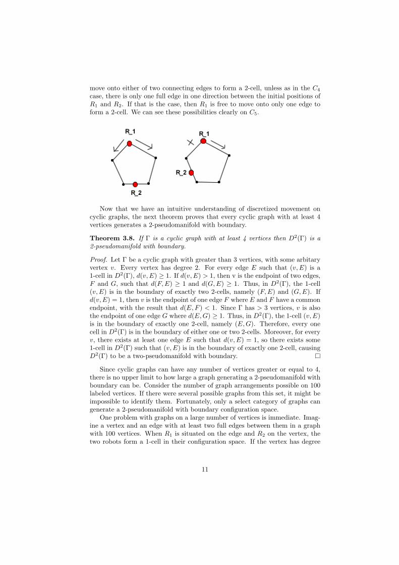
move onto either of two connecting edges to form a 2-cell, unless as in the C4

case, there is only one full edge in one direction between the initial positions ofR1 and R2. If that is the case, then R1 is free to move onto only one edge toform a 2-cell. We can see these possibilities clearly on C5.

Now that we have an intuitive understanding of discretized movement oncyclic graphs, the next theorem proves that every cyclic graph with at least 4vertices generates a 2-pseudomanifold with boundary.

Theorem 3.8. If Γ is a cyclic graph with at least 4 vertices then D2(Γ) is a2-pseudomanifold with boundary.

Proof. Let Γ be a cyclic graph with greater than 3 vertices, with some arbitaryvertex v. Every vertex has degree 2. For every edge E such that (v,E) is a1-cell in D2(Γ), d(v,E) ≥ 1. If d(v,E) > 1, then v is the endpoint of two edges,F and G, such that d(F,E) ≥ 1 and d(G,E) ≥ 1. Thus, in D2(Γ), the 1-cell(v,E) is in the boundary of exactly two 2-cells, namely (F,E) and (G,E). Ifd(v,E) = 1, then v is the endpoint of one edge F where E and F have a commonendpoint, with the result that d(E,F ) < 1. Since Γ has > 3 vertices, v is alsothe endpoint of one edge G where d(E,G) ≥ 1. Thus, in D2(Γ), the 1-cell (v,E)is in the boundary of exactly one 2-cell, namely (E,G). Therefore, every onecell in D2(Γ) is in the boundary of either one or two 2-cells. Moreover, for everyv, there exists at least one edge E such that d(v,E) = 1, so there exists some1-cell in D2(Γ) such that (v,E) is in the boundary of exactly one 2-cell, causingD2(Γ) to be a two-pseudomanifold with boundary.

Since cyclic graphs can have any number of vertices greater or equal to 4,there is no upper limit to how large a graph generating a 2-pseudomanifold withboundary can be. Consider the number of graph arrangements possible on 100labeled vertices. If there were several possible graphs from this set, it might beimpossible to identify them. Fortunately, only a select category of graphs cangenerate a 2-pseudomanifold with boundary configuration space.

One problem with graphs on a large number of vertices is immediate. Imag-ine a vertex and an edge with at least two full edges between them in a graphwith 100 vertices. When R1 is situated on the edge and R2 on the vertex, thetwo robots form a 1-cell in their configuration space. If the vertex has degree

11

greater than 2, then R2 is free to move onto more than two edges, so that theoriginal 1-cell is in the boundary of more than two 2-cells.

The following theorem and corollary prove that for a graph on 7 or morevertices, the only vertex arrangement that eliminates the above difficulty is thatof the cyclic graph.

Theorem 3.9. If Γ is a simple connected graph on at least 7 vertices with aconfiguration space that is a 2-pseudomanifold with boundary, then every vertexin Γ has degree at most two.

Proof. Let Γ be a simple connected graph on n ≥ 7 vertices with a 2-pseudomanifoldconfiguration space with boundary. Suppose that Γ has a vertex v of degreem ≥ 3. We will consider the cases where m = 3, 4 ≤ m ≤ 5, and m ≥ 6, andshow that for each case, D2(Γ) is not a 2-pseudomanifold with boundary.

Case 1: Vertex v has degree 3.If v has degree 3, being adjacent to vertices x, y and z, then there remain

n − 4 vertices that are not adjacent to v. Either at least two of these n − 4vertices are adjacent, or else no two are adjacent. If any two are adjacent, theyform an edge E such that d(E, vx) ≥ 1, d(E, vy) ≥ 1, and d(E, vz) ≥ 1. Thusthe 1-cell (v,E) in D2(Γ) is in the boundary of three 2 cells, namely (E, vx),(E, vy), and (E, vz) and D2(Γ) is not a 2-pseudomanifold.

If no two of the n− 4 vertices not adjacent to v are adjacent to one another,then let the n − 4 vertices along with vertex v be in a subset A, and let the 3vertices adjacent to v be in a subset B, such that A∪B = Γ and A∩B = φ. Acontains at least 4 vertices, such that v has degree 3 and every other vertex has

degree ≥ 2. The sum of vertex degrees over A,∑

vi∈A

deg(vi) ≥ 3+(3∗2) = 9. No

two vertices in A are adjacent, thus there at at least 9 edges with one endpointin A and the other endpoint in B. Since there are exactly 3 vertices in Y and9 ÷ 3 = 3, there exists a vertex in Y adjacent to at least 3 vertices in X, oneof those being v. Without loss of generality, say that vertex x ∈ B is adjacentto v, and at least two additional vertices u and w. As A has at least 4 vertices,there exists at least one more vertex in A which may or may not be adjacentto x, label this vertex s. Since every vertex has degree ≥ 2, vertex s must beadjacent to at least one vertex not x and since s ∈ A, s is not adjacent to anyother vertex in A. Thus s is adjacent to at least one of y or z. Now there existat least 3 edges with endpoint x but not endpoint s, y, or z, so without loss ofgenerality, say that s is adjacent to z. Then in D2(Γ), the 1-cell (x, sz) is in theboundary of three 2-cells, namely (xv, sz), (xu, sz), and (xw, sz) and D2(Γ) isnot a 2-pseudomanifold.

Case 2: Vertex v has degree 4 ≤ m ≤ 5.Vertex v is adjacent to either 4 or 5 vertices, and not every vertex in Γ is

adjacent to v. Since Γ is connected, at least one vertex not adjacent to v mustbe adjacent to some vertex that is also adjacent to v. Say that vertex u is notadjacent to v, but is adjacent to x, where x is adjacent to v. Then there are atleast 3 edges with endpoint v, but not endpoints u or x. Therefore in D2(Γ),

12

the 1-cell (v, xu) is in the boundary of at least three 2-cells and D2(Γ) is not a2-pseudomanifold.

Case 3: Vertex v has degree ≥ 6.Either v is adjacent to every other vertex in Γ or else there exists at least

one vertex not adjacent to v. If v is adjacent to every other vertex, then sinceevery vertex has degree ≥ 2, for vertex x 6= v, then x is adjacent to at least oneother vertex y. There are at least 4 edges with endpoint v, but not endpoints xor y. Therefore in D2(Γ), the 1-cell (v, xu) is in the boundary of at least four2-cells and D2(Γ) is not a 2-pseudomanifold.

If there exists at least one vertex not adjacent v, then since Γ is connected,at least one vertex not adjacent to v must be adjacent to some vertex that isalso adjacent to v. Say that vertex u is not adjacent to v, but is adjacent to x,where x is adjacent to v. Then there are at least 5 edges with endpoint v, butnot endpoints u or x. Therefore in D2(Γ), the 1-cell (v, xu) is in the boundaryof at least five 2-cells and D2(Γ) is not a 2-pseudomanifold.

Having ruled out the cases where v has degree > 2, we conclude that ifD2(Γ) is a 2-pseudomanifold with boundary, then v has degree ≤ 2 for all v inΓ.

Corollary 3.10. If Γ is a simple, connected graph on n ≥ 7 vertices with a con-figuration space that is a two-pseudomanifold configuration space with boundary,then Γ is the cyclic graph on n vertices.

Proof. Let Γ be a simple, connected graph on n ≥ 7 vertices with a two-pseudomanifold configuration space with boundary. By Theorem 3.9, everyvertex in Γ has degree ≤ 2, and by Theorem 3.1, every vertex has degree ≥ 2.Therefore, every vertex must have exactly degree 2, making Γ the cyclic graphon n vertices.

Now that we have a lower vertex limit for all graphs and an upper vertexlimit for all graphs excluding cyclics, we can classify graphs according to theirnumber of vertices. Graphs generating 2-pseudomanifolds with boundary musthave 4, 5, or 6 vertices. Recall that graphs on 5 and 6 vertices must be simple.Beginning with graphs on 6 vertices, unworkable cases will be eliminated anddesirable graphs identified.

3.3 Graphs on Six Vertices

Two graphs on 6 vertices whose configuration spaces are special structures havealready been identified. D2(K3,3) is a 2-manifold, the 4-holed torus, and D2(C6)is a 2-pseudomanifold with boundary.

As there are many vertex arrangements possible, a few preliminary lem-mas greatly narrow down the possibilities. Note that they hold true for 2-pseudomanifolds both with and without boundary.

Lemma 3.11. Let Γ be a simple, connected graph on 6 vertices. If D2(Γ) is a2-pseudomanifold configuration space, either with or without boundary, then forany vertex v in Γ, the degree of v is either 2 or 3.

13

Proof. Let Γ be a simple, connected graph on 6 vertices. The maximum degreeof any vertex is 5. Assume that vertex v has degree 5, so that every other vertexin Γ is adjacent to v. Since every vertex has degree ≥ 2, some two vertices x andy adjacent to v must be the endpoints of some edge E such that d(v,E) = 1.Then there are exactly three edges with endpoint v but not endpoint x or y,labeled F , G, and H, such that d(E,F ) = 1, d(E,G) = 1, and d(E,H) = 1.Therefore, in D2(Γ), the 1-cell (v,E) is in the boundary of three 2-cells, namely(E,F ), (E,G), and (E,H), and D2(Γ) is not a two-psuedomanifold.

Next assume that vertex v has degree 4, so that there is exactly one vertexw not adjacent to v. Since Γ is connected, w must be adjacent to some vertexx thus creating edge E. Since every vertex not w is adjacent to v, x is adjacentto v, so d(v,E) = 1. There are exactly three edges with v but not x or w asan endpoint, labeled F , G, and H. Therefore, in D2(Γ), the 1-cell (v,E) is inthe boundary of three 2-cells, namely (E,F ), (E,G), and (E,H), and D2(Γ) isnot a two-psuedomanifold. As v cannot have degree 4 or 5 if D2(Γ) is to be atwo-pseudomanifold, every vertex v in Γ has degree ≤ 3.

We have previously proven in Corollary 3.2 that if D2(Γ) is a two-pseudomanifoldwith or without boundary, then every vertex in the simple, connected graph Γhas degree at least 2. Thus, every vertex in Γ has either degree 2 or degree3.

Lemma 3.12. Let Γ be a simple, connected graph on 6 vertices. If every vertexin Γ has either degree 2 or 3, then there is an even number of vertices withdegree 3 in Γ.

Proof. Denote deg(Γ) to be the sum of vertex degrees over all vertices in Γ,6∑

i=1

deg(vi), and E(Γ) to be the number of edges contained in Γ. deg(Γ) =

2 × E(Γ), since each edge has two vertices as endpoints. Thus deg(Γ) is even.Suppose that the number n of vertices in Γ having degree 3 is odd, and that allother vertices have degree 2. deg(Γ) = (3 × n) + (2 × (6 − n)). The productof two odd integers is odd, so deg(Γ) is the sum of an odd integer and an eveninteger, making deg(Γ) odd, a contradiction as deg(Γ) has been determined tobe even. Therefore, there is an even number of vertices in Γ with degree 3,either 0, 2, 4, or 6.

Using the results of the proceding lemma, we examine the graph on 6 verticescase by case. We learn that besides C6, there are just two other graphs on 6vertices which generate a 2-pseudomanifold with boundary.

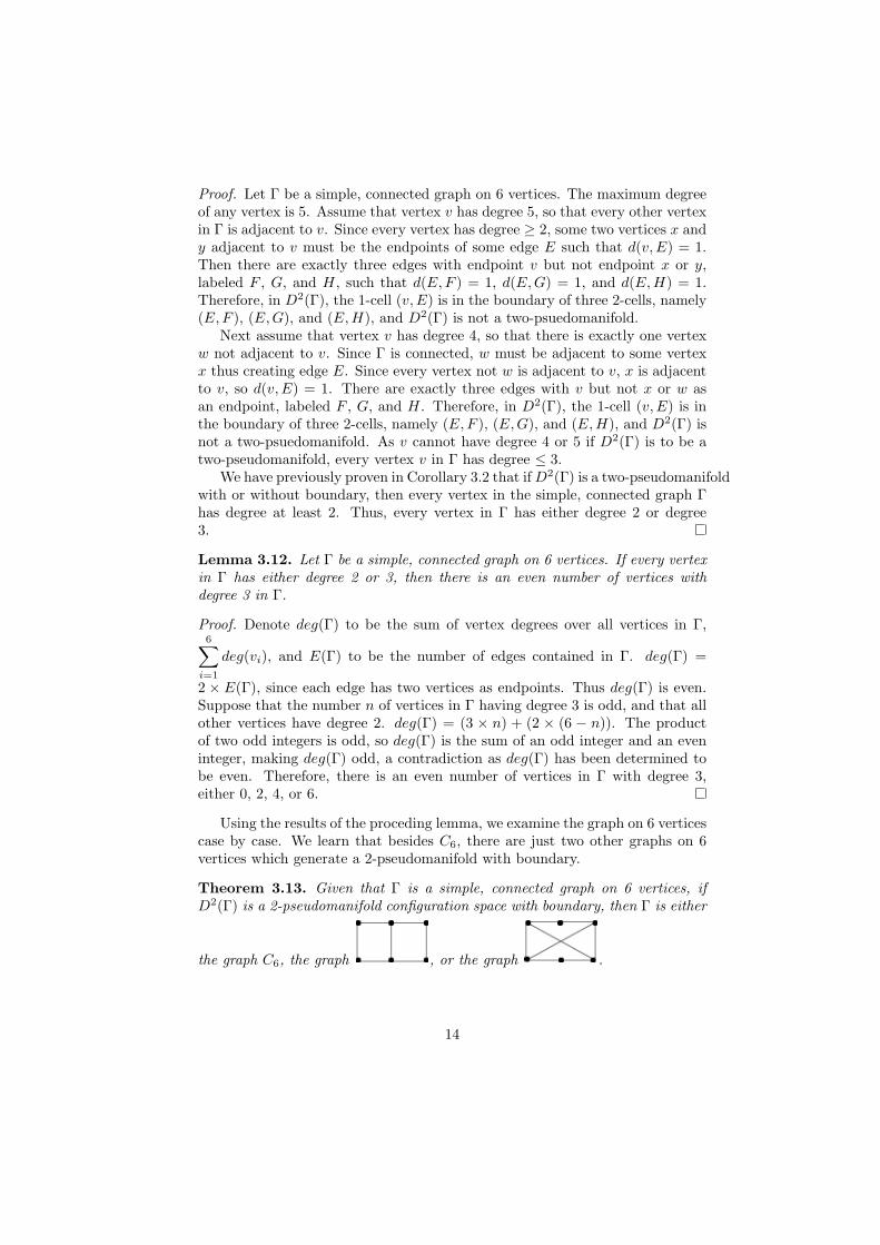
Theorem 3.13. Given that Γ is a simple, connected graph on 6 vertices, ifD2(Γ) is a 2-pseudomanifold configuration space with boundary, then Γ is either

the graph C6, the graph , or the graph .

14

Proof. We will demonstrate which specific graphs with 6 vertices have con-figuration spaces that are 2-pseudomanifolds. Suppose that D2(Γ) is a 2-pseudomanifold configuration space with boundary. From the two previouslemmas, every vertex of Γ has either degree 2 or 3, and there is an even numberof vertices in Γ with degree 3.

Case 1: Γ has no vertices of degree 3.If Γ has no vertices with degree 3, every vertex must have degree 2. Then Γ

is C6, the cyclic graph with 6 vertices, which has been proven in Theorem 3.8to be a 2-pseudomanifold with boundary.

Case 2: Γ has two vertices of degree 3 and four of degree 2.Let Γ have two vertices of degree 3, labeled v and w, and four of degree 2,

u, x, y, and z. We will now show that v and w are adjacent. Suppose thatv is not adjacent to w, so that v is adjacent to x, y and z. Then w cannotalso be adjacent to x, y and z, giving w degree 3 and x, y and z each degree2, because, with available degrees exhausted, there will remain one vertex unot adjacent to any other vertex in Γ. Thus, w must be adjacent to u, whereu is not adjacent to v, forming edge E. As neither w nor u are adjacent tov, d(v,E) ≥ 1, corresponding to 1-cell (v,E) in D2(Γ). The three edges withendpoint v have endpoints x, y and z respectively. Since no common endpointsare shared with E, d(vx,E) ≥ 1, d(vy,E) ≥ 1 and d(vz,E) ≥ 1. In D2(Γ), the1-cell (v,E) is in the boundary of three 2-cells, namely (vx,E), (vy,E), and(vz,E), so that D2(Γ) is not a 2-psuedomanifold. Therefore, v is adjacent to w.

Letting v be adjacent to w, we will now show that no vertex in Γ is adjacentto both v and w. As v has degree 3, let v be adjacent to x and y. w mustbe adjacent to two additional vertices. w cannot be adjacent to both x and y,giving v and w degree 3 and x and y degree 2, because the two vertices u and zwill then be unable to form edges with any other vertices. Suppose then that wis adjacent to one vertex x which is also adjacent to v. Immediately we see thatvertex x has degree 2 and is in the 3-cycle x−v−w, resulting in a configurationspace which is not a 2-pseudomanifold, according to Corollary 3.4,. Thus, inD2(Γ), 1-cell (x, vw) is in the boundary of no 2-cells, so that D2(Γ) is not a2-pseudomanifold. Therefore, no vertex in Γ is adjacent to both v and w, thevertices of degree 3.

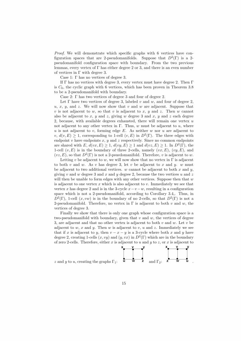
Finally we show that there is only one graph whose configuration space is atwo-pseudomanifold with boundary, given that v and w, the vertices of degree3, are adjacent and that no other vertex is adjacent to both v and w. Let v beadjacent to w, x and y. Then w is adjacent to v, u and z. Immediately we seethat if x is adjacent to y, then v − x − y is a 3-cycle where both x and y havedegree 2, creating 1-cells (x, vy) and (y, vx) in D2(Γ) which are in the boundaryof zero 2-cells. Therefore, either x is adjacent to u and y to z, or x is adjacent to

z and y to u, creating the graphs Γ1: and Γ2: .

15

Since the labeling of the graphs is arbitrary, Γ1∼= Γ2

∼= Γ = . Itis easy to check that for every vertex v and edge E with d(v,E) ≥ 1, v is theendpoint of either one or two edges F , G with d(E,F ) ≥ 1 and d(E,G) ≥ 1, sothat every 1-cell (v,E) in D2(Γ) is in the boundary of either one or two 2-cells.

Thus, Γ = with two vertices of degree 3 is a 2-pseudomanifold withboundary.

Case 3: Γ has four vertices of degree 3 and two vertices of degree 2.Let Γ have four vertices of degree 3, labeled w, x, y, and z, and two vertices

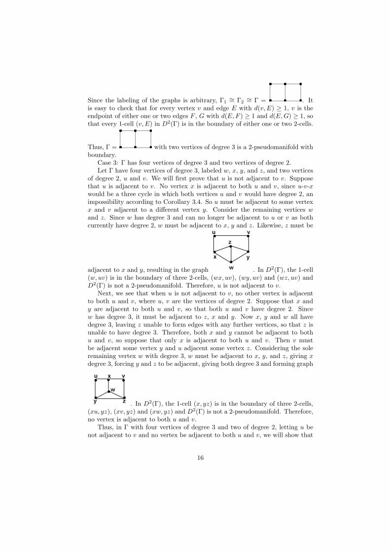
of degree 2, u and v. We will first prove that u is not adjacent to v. Supposethat u is adjacent to v. No vertex x is adjacent to both u and v, since u-v-xwould be a three cycle in which both vertices u and v would have degree 2, animpossibility according to Corollary 3.4. So u must be adjacent to some vertexx and v adjacent to a different vertex y. Consider the remaining vertices wand z. Since w has degree 3 and can no longer be adjacent to u or v as bothcurrently have degree 2, w must be adjacent to x, y and z. Likewise, z must be

adjacent to x and y, resulting in the graph . In D2(Γ), the 1-cell(w, uv) is in the boundary of three 2-cells, (wx, uv), (wy, uv) and (wz, uv) andD2(Γ) is not a 2-pseudomanifold. Therefore, u is not adjacent to v.

Next, we see that when u is not adjacent to v, no other vertex is adjacentto both u and v, where u, v are the vertices of degree 2. Suppose that x andy are adjacent to both u and v, so that both u and v have degree 2. Sincew has degree 3, it must be adjacent to z, x and y. Now x, y and w all havedegree 3, leaving z unable to form edges with any further vertices, so that z isunable to have degree 3. Therefore, both x and y cannot be adjacent to bothu and v, so suppose that only x is adjacent to both u and v. Then v mustbe adjacent some vertex y and u adjacent some vertex z. Considering the soleremaining vertex w with degree 3, w must be adjacent to x, y, and z, giving xdegree 3, forcing y and z to be adjacent, giving both degree 3 and forming graph

. In D2(Γ), the 1-cell (x, yz) is in the boundary of three 2-cells,(xu, yz), (xv, yz) and (xw, yz) and D2(Γ) is not a 2-pseudomanifold. Therefore,no vertex is adjacent to both u and v.

Thus, in Γ with four vertices of degree 3 and two of degree 2, letting u benot adjacent to v and no vertex be adjacent to both u and v, we will show that

16

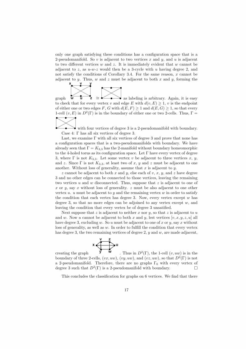
only one graph satisfying these conditions has a configuration space that is a2-pseudomanifold. So v is adjacent to two vertices x and y, and u is adjacentto two different vertices w and z. It is immediately evident that w cannot beadjacent to z, as u-w-z would then be a 3-cycle with u having degree 2, andnot satisfy the conditions of Corollary 3.4. For the same reason, x cannot beadjacent to y. Thus, w and z must be adjacent to both x and y, forming the

graph ∼= as labeling is arbitrary. Again, it is easyto check that for every vertex v and edge E with d(v,E) ≥ 1, v is the endpointof either one or two edges F , G with d(E,F ) ≥ 1 and d(E,G) ≥ 1, so that every1-cell (v,E) in D2(Γ) is in the boundary of either one or two 2-cells. Thus, Γ =

with four vertices of degree 3 is a 2-pseudomanifold with boundary.Case 4: Γ has all six vertices of degree 3.Last, we examine Γ with all six vertices of degree 3 and prove that none has

a configuration spaces that is a two-pseudomanifolds with boundary. We havealready seen that Γ = K3,3 has the 2-manifold without boundary homeomorphicto the 4-holed torus as its configuration space. Let Γ have every vertex of degree3, where Γ is not K3,3. Let some vertex v be adjacent to three vertices x, y,and z. Since Γ is not K3,3, at least two of x, y and z must be adjacent to oneanother. Without loss of generality, assume that x is adjacent to y.

z cannot be adjacent to both x and y, else each of v, x, y, and z have degree3 and no other edges can be connected to those vertices, leaving the remainingtwo vertices u and w disconnected. Thus, suppose that z is adjacent to one ofx or y, say x without loss of generality. z must be also adjacent to one othervertex u. u must be adjacent to y and the remaining vertex w in order to satisfythe condition that each vertex has degree 3. Now, every vertex except w hasdegree 3, so that no more edges can be adjoined to any vertex except w, andleaving the condition that every vertex be of degree 3 unsatified.

Next suppose that z is adjacent to neither x nor y, so that z is adjacent to uand w. Now u cannot be adjacent to both x and y, lest vertices [v, x, y, z, u] allhave degree 3, excluding w. So u must be adjacent to one of x or y, say x withoutloss of generality, as well as w. In order to fulfill the condition that every vertexhas degree 3, the two remaining vertices of degree 2, y and w, are made adjacent,

creating the graph . Thus in D2(Γ), the 1-cell (v, uw) is in theboundary of three 2-cells, (vx, uw), (vy, uw), and (vz, uw), so that D2(Γ) is nota 2-pseudomanifold. Therefore, there are no graphs Γ6 with every vertex ofdegree 3 such that D2(Γ) is a 2-pseudomanifold with boundary.

This concludes the classification for graphs on 6 vertices. We find that there

17

might not be a great number of configuration space generating graphs on lessthan 7 vertices that result in 2-pseudomanifolds with boundary. The remainingclassifications have shorter proofs and depend more upon already developedtheorems.

3.4 Graphs on Five Vertices

We mentioned earlier that Corollaries 3.2 and 3.4 would be crucial in laterproofs. It turns out that these two necessary conditions are also sufficient fordefining 2-pseudomanifold generating graphs on 5 vertices. The following the-orem proves their sufficiency, but does not outline the vertex arrangement ofevery graph that meets the criteria for a 2-pseudomanifold configuration space.We recall the the configuration space D2(K5) is a 2-manifold, specifically the6-holed torus.

Theorem 3.14. Let Γ be a simple connected graph on 5 vertices, with everyvertex having degree at least 2. Then Γ has a 2-pseudomanifold configurationspace with possible boundary if and only if no vertex in a 3-cycle has degree 2.

Proof. If D2(Γ) is a two-pseudomanifold, then no vertex in a 3-cycle has degree2 in Γ, a simple connected graph on 5 vertices. This has been proven for aconnected graph on any number of vertices in Theorem 3.3.

Conversely, because Γ has 5 vertices, any vertex v must have degree 2, 3,or 4. We will show that for each permissible degree of an arbitrary vertex v,if no vertex in any 3-cycle of Γ has degree 2, then where edge E is such thatd(v,E) ≥ 1, the 1-cell (v,E) is in the boundary of either one or two 2-cells.

Suppose that no vertex in any 3-cycle of Γ has degree 2.Case 1: Vertex v has degree 2.Because Γ is connected, Γ contains edges that do not have v as an endpoing.

Suppose that E is one such edge in Γ such that (v,E) is a 1-cell in D2(Γ).If there is no edge F with endpoint v such that d(E,F ) ≥ 1, then v is in a3-cycle with v adjacent to the endpoints of E. This is not permissible by thesupposition. Thus v must be the endpoint of at least one edge F such thatd(E,F ) ≥ 1. Specifically, if d(v,E) = 1, then v is adjacent to one endpoint ofE, and is the endpoint of exactly one edge F with d(E,F ) ≥ 1. Thus, in D2(Γ),the 1-cell (v,E) is in the boundary of one 2-cell (E,F ). If d(v,E) > 1, then v isthe endpoint of exactly two edges F and G with d(E,F ) ≥ 1 and d(E,G) ≥ 1.Similarly, in D2(Γ), (v,E) is in the boundary of two 2-cells, (E,F ) and (F,G).v is never the endpoint of three or more such edges since the degree of v is 2.Therefore, (v,E) is in the boundary of either one or two 2-cells.

Case 2: Vertex v has degree 3.Since Γ has 5 vertices, v is adjacent to three vertices x, y, and z, but not to

one vertex w. As in Case 1, Γ has edges that do not have v as an endpoint. If Edoes not have endpoint w, then both endpoints of E are adjacent to v. Withoutloss of generality, denote x and y the endpoints of E with the consequencethat d(E, vx) < 1 and d(E, vy) < 1. Since v and z are not endpoints of E,d(E, vz) = 1. Therefore, in D2(Γ), the 1-cell (v,E) is in the boundary of the

18

2-cell (E, vz) and in the boundary of no other 2-cell. If w is an endpoint of E,then E has another endpoint that is adjacent to v. Without loss of generality,denote x an endpoint of E with the consequence that d(E, vx) < 1. Now neitherv, y, nor z is an endpoint of E, so d(E, vy) ≥ 1 and d(E, vz) ≥ 1. Accordingly,in D2(Γ), the 1-cell (v,E) is in the boundary of exactly two 2-cells, (E, vy) and(E, vz). Therefore (v,E) is in the boundary of either one or two 2-cells.

Case 3: Vertex v has degree 4.v is adjacent to every other vertex in Γ, namely w, x, y, and z. Every edge

E such that d(v,E) ≥ 1 has endpoints that are both adjacent to v. Such anedge exists because the degree of every vertex is ≥ 2. Without loss of generality,denote x and y the endpoints of E. Then d(E, vw) = 1 and d(E, vz) = 1, butd(E, vx) < 1 and d(E, vy) < 1. Therefore, in D2(Γ), the 1-cell (v,E) is in theboundary of exactly two 2-cells, (E, vw) and (E, vz).

In conclusion, if no vertex in Γ which is in a 3-cycle has degree 2, then anyvertex v and edge E such that d(v,E) ≥ 1 corresponds to a 1-cell (v,E) inD2(Γ) that is in the boundary of either one or two 2-cells, so that D2(Γ) is a2-pseudomanifold.

Note that the proof has been written for graphs generating 2-pseudomanifoldconfiguration spaces with possible boundary. Under the suppositions of theproof, it is impossible to rule out that a graph configuration space may be a 2-pseudomanifold without boundary. However, we know from earlier work that K5

is the only graph on five vertices giving rise to a 2-manifold or 2-pseudomanifoldwithout boundary. We must then conclude that any other graph on 5 verticesmeeting the criteria given in the theorem generates a 2-pseudomanifold withboundary.

Although the theorem does not identify by vertex arrangement which graphsmeet its criteria, these graphs are easy to identify. Checking to see that no vertexhas degree 0 or 1 is immediate. Verifying that no vertex in a 3-cycle has degree2 is best done by identifying all vertices with degree 2, then confirming for eachthat its two adjacent vertices are not mutual endpoints of a common edge.

3.5 Graphs on Four Vertices

The set of graphs on 4 vertices differ from the previous classifications by con-taining both simple and non-simple graphs. We begin with the simple graphs,which also use Corollaries 3.2 and 3.4 as sufficient conditions for generating a2-pseudomanifold with boundary configuration space. Because there are fewercases, we specify which two specific graphs fall under this classification.

Theorem 3.15. If Γ is a simple connected graph on 4 vertices such that everyvertex has degree at least two and such that no vertex in a 3-cycle has degree 2,then the configuration space D2(Γ) is a 2-pseudomanifold with boundary. Theonly two such graphs are the cyclic graph C4 and the complete graph K4.

Proof. Let Γ be a simple connected graph on 4 vertices such that every vertexhas degree ≥ 2 and such that no vertex in a 3-cycle has degree 2. Label the

19

vertices of Γ as v, x, y and z. Vertex v is adjacent to either 2 or 3 of the othervertices. Suppose that v is adjacent to three vertices x, y and z. Each of x,y and z must be made adjacent to at least one other vertex. Without loss ofgenerality, let x and y be adjacent. Now v − x − y is a 3-cycle in which bothx and y have degree 2. Thus both x and y must be adjacent to the remainingvertex z. The resulting graph is the complete graph on 4 vertices, K4 and nomore edges may be added.

In the complete graph, every vertex is adjacent to every other vertex, so forany three vertices v, x and y in K4, d(v, x) = 1 and d(v, y) = 1 so that (v, xy)is a 1-cell in D2(K4). Now v is adjacent to exactly one more vertex z, so that(v, xy) is in the boundary of exactly the one 2-cell (vz, xy) in D2(Γ). ThereforeD2(Γ) is a 2-pseudomanifold with boundary.

Next suppose that v is adjacent to two vertices x and y. Vertex x can notbe adjacent to y, else v − x− y is a 3-cycle in which v has degree 2. So for eachvertex to have degree ≥ 2, both x and y must be adjacent to the remainingvertex z. Vertex z cannot be adjacent to any more vertices, as it is not adjacentto v. The resulting graph is the cyclic graph on 4 vertices, C4, which is a2-pseudomanifold with boundary, as proven in Theorem 3.8.

Corollary 3.16. Let Γ be a simple connected graph on 4 vertices. If D2(Γ) is a2-pseudomanifold with boundary, i.e. Γ is C4 or K4, then every 1-cell in D2(Γ)is in the boundary of exactly one 2-cell.

Proof. It has been proven in Theorem 3.15 that for the four vertices arbitrarilylabeled v, x, y and z in K4, (v, xy) is a 1-cell in D2(K4) which is in the boundaryof exactly the 2-cell (vz, xy). Let the 4-cycle C4 have arbitrarily ordered verticesv − x− y − z. Thus, (v, xy) is a 1-cell in D2(C4) in the boundary of exactly the2-cell (vz, xy). Likewise, (v, yz) is a 1-cell in the boundary of exactly the 2-cell(vx, yz). Because of the symmetries of K4 and C4, these relationships hold forevery arbitrary labeling.

Moving into the non-simple graph cases, the next lemma addresses multipleedges. Although a pair of vertices in a non-simple graph may normally be mutualendpoints for any number of common edges, a 2-pseudomanifold generatinggraph is restricted to two common edges per pair of vertices.

Lemma 3.17. Let D2(Γ) be a 2-pseudomanifold configuration space, with orwithout boundary. If Γ is a non-simple, connected graph, then no pair of end-points in Γ serves as the endpoint set of more than two edges.

Proof. Suppose that a non-simple, connected graph Γ has a pair of vertices xand y with m-tuple edges {E1, E2, ..., Em}, such that m ≥ 3. If there existsedge F such that neither x nor y is an endpoint of F , then d(Ek, F ) ≥ 1 for all1 ≥ k ≥ m. Thus the 1-cell (x, F ) in D2(Γ) is in the boundary of m 2-cells,m ≥ 3, so that D2(Γ) is not a 2-pseudomanifold. Suppose that no such edgeF exists, so that every vertex v in Γ must be adjacent to x or y. In fact, sinceevery vertex must be adjacent to at least 2 other vertices, then every vertex vmust be adjacent to both x and y. For all such edges Fi and Gj with respective

20

endpoints x, v and y, v, then d(Ek, Fi) < 1 and d(Ek, Gj) < 1 for all 1 ≥ k ≥ m.Thus the 1-cells (v,Ek), 1 ≥ k ≥ m, are in the boundary of no 2-cells in D2(Γ)and D2(Γ) is not a 2-pseudomanifold. Therefore, no pair of endpoints in Γ havem-tuple edges such that m ≥ 3.

Finally we come to our last classification. Non-simple graphs Γ on 4 verticesare exactly the graphs that can be formed from C4 or K4 by doubling any subsetof the C4 or K4 edges.

Theorem 3.18. Let Γ be a non-simple connected graph on 4 vertices, whereany pair of vertices in Γ are the mutual endpoints of at most double edges. Γhas a 2-pseudomanifold configuration space, with or without boundary, if andonly if the non-simple graph Γ has the same vertex adjacencies as the simplegraph C4 or the simple graph K4.

Proof. Let Λ be a simple connected graph on 4 vertices. Suppose that Λ isneither C4 nor K4. From the conditions of Theorem 3.15, we know that Λeither contains a vertex with degree less than 2 or that Λ has a vertex of degree2 within a 3-cycle. First suppose that Λ contains a vertex vΛ with degree < 2.In a simple connected graph, this implies that vΛ is adjacent to only one othervertex. For any non-simple connected graph Γ on 4 vertices, where Γ and Λ havethe same vertex adjacencies, since vΛ is adjacent to only one other vertex, thenvΓ is also adjacent to one other vertex. Then D2(Γ) is not a 2-pseudomanifold,with or without boundary, since Γ contains a vertex which is adjacent to onlyone other vertex.

Next suppose that Λ contains a vertex vΛ of degree 2 within a 3-cycle vΛ −xΛ − yΛ. This implies that v is adjacent to exactly two other vertices, xΛ andyΛ. For any non-simple connected graph Γ on 4 vertices, where Γ and Λ havethe same vertex adjacencies, since vΛ is adjacent to exactly xΛ and yΛ, then vΓ

is also adjacent to exactly xΓ and yΓ. Thus Γ contains at least one 3-cycle onvertices vΓ, xΓ, and yΓ where vΓ is adjacent to exactly 2 vertices. So D2(Γ) isnot a 2-pseudomanifold. This proves that if Λ is a graph such that D2(Λ) is nota 2-pseudomanifold then any non-simple connected graph Γ having the samevertex adjacencies as Λ also does not have a 2-pseudomanifold configurationspace. Therefore, if a non-simple connected graph on 4 vertices, Γ, has a 2-pseudomanifold configuration space, then there exists a simple graph Λ on 4vertices, having a 2-pseudomanifold configuration space with boundary, suchthat Λ and Γ have the same vertex adjacencies.

Conversely, any graph Γ on 4 vertices having the same vertex adjacencies asC4 or K4 has the properties that every vertex is adjacent to at least two othervertices, and that no vertex in a 3-cycle is adjacent to exactly two other vertices,since the same must hold true for Λ as seen in Theorem 3.15.

Suppose that Γ is some non-simple graph with at most double edges where Γhas the same vertex adjacencies as C4. Arbitrarily order the vertex adjacenciesv − x − y − z. There exists at least one edge E, and possibly a second edgeF with endpoints x and y, and at least one edge G and possibly a second Hwith endpoints v and z. Thus, in D2(Γ), the 1-cell (v,E) is in the boundary

21

of either one or two 2-cells (G,E) and (H,E). If edge F exists, then the 1-cell(v, F ) is also in the boundary of one or two two 2-cells (G,F ) and (H,F ). Asimilar proof holds where there exists at least one edge K, and possibly a secondL with endpoints z and y, and at least one edge M and possibly a second Nwith endpoints v and x. Then, in D2(Γ), the 1-cell (v,K) is in the boundary ofeither one or two 2-cells (M,K) and (N,K), and if L exists, the one cell (v, L)is also in the boundary of one or two 2-cells (M,L) and (N,L). Due to thesymmetry and arbitrary ordering of C4 = Λ, similar relationships hold for anychosen vertex. Therefore, every 1-cell is in the boundary of at least one and atmost two 2-cells in D2(Γ), where Γ and C4 have the same vertex adjacenciesand Γ has at most double edges.

Suppose that Γ is some nonsimple graph with at most double edges whereΓ has the same vertex adjacencies as K4. Every vertex in Γ is adjacent to everyother vertex by at least one edge. For any three vertices v, x and y, the distancebetween each is exactly one. There exists at least one edge E and possibly asecond edge F with endpoints x and y, creating possible 1-cells (v,E) and (v, F )in D2(Γ). Then v is adjacent to exactly one other vertex z, with either one ortwo edges G and H having endpoints v and z. Therefore, the 1-cell (v,E) isin the boundary of either one or two 2-cells in D2(Γ), (G,E) and (H,E), andif edge F exists, then the 1-cell (v, F ) is in the boundary of either one or two2-cells, (G,F ) and (H,F ). Since K4 is completely symmetrical at every vertex,similar relationships hold for any chosen vertex. Therefore, every 1-cell is inthe boundary of at least one and at most two 2-cells in D2(Γ), where Γ and K4

have the same vertex adjacencies and Γ has at most double edges.

Again, we note that the theorem includes 2-pseudomanifold configurationspaces, both with and without boundary. We know that the graphs generating2-pseudomanifolds without boundary are doubled C4 and doubled K4 and noneother, so we can conclude that every other graph in the set besides these twogenerates a 2-pseudomanifold configuration space with boundary.

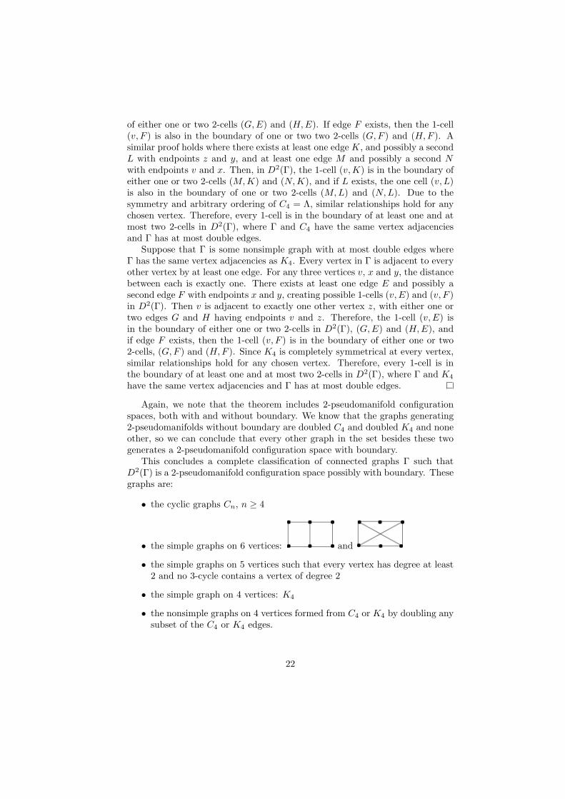
This concludes a complete classification of connected graphs Γ such thatD2(Γ) is a 2-pseudomanifold configuration space possibly with boundary. Thesegraphs are:

• the cyclic graphs Cn, n ≥ 4

• the simple graphs on 6 vertices: and

• the simple graphs on 5 vertices such that every vertex has degree at least2 and no 3-cycle contains a vertex of degree 2

• the simple graph on 4 vertices: K4

• the nonsimple graphs on 4 vertices formed from C4 or K4 by doubling anysubset of the C4 or K4 edges.

22

4 The Fundamental Group of a Configuration

Space

As we have seen, the question of whether a graph configuration space is a pseudo-manifold can be answered by local combinatorial reasoning. When the configu-ration space is an orientable 2-dimensional manifold, the space can be identifiedby similar reasoning because the Euler characteristic provides a complete clas-sification of such manifolds. In this way, the space D2(K5) is known to bethe 6-holed torus and the space D2(K3,3) to be the 4-holed torus. In general,classification depends on more sophisticated algebraic invariants, such as thefundamental group.

A catalogue of 2-dimensional pseudomanifolds with boundary can never beas straightforward and useful as the catalogue of 2-dimensional manifolds. Fromany 2-dimensional pseudomanifold one can make a new one by identifying ver-tices. However, independent of any application to classification, the fundamen-tal group of a graph configuration space remains interesting. Such fundamentalgroups are an analogue of the better known braid groups, which are funda-mental groups of configuration spaces of points in the plane. The braid groupassociated with configuration of a pair of points in the plane can quickly be seento be isomorphic to Z. In contrast, the fundamental group of the configurationspace of two points on a graph can be much more interesting due to the naturaltopology of the graph.

In what follows, we illustrate the technique needed to calculate these funda-mental groups by calculating the fundamental group of D2(K5).

4.1 Fibrations

Over each distinct vertex or edge in a graph Γ, a fibration in D2Γ may be createdby fixing one robot on the given point or edge, while allowing the second robotto move freely upon other permissible paths in the graph, namely those verticesand edges which are at least of distance one away from the given vertex or edge.In the specific graph K5, when one robot is fixed on any given vertex, the secondrobot is free to move around the remaining four points and the edges connectingthem to one another. Likewise, when one robot is fixed on any given edge, thesecond robot is permitted to move on the trianglar path connecting the threevertices that are not endpoints of the given edge.

Visualizations of a fibration over a point and an edge are given in Figures 1and 2 in the Appendix of Figures. The vertices in the resulting space D2Γ arelabeled with the position of Robot 1 then the position of Robot 2, separated bya comma.

The entire configuration space can be viewed as a union of these individualfibrations. The local topology of each fibration gives a clearer picture of theglobal topology of the manifold. In D2(K5), each edge fibration is a triangu-lar tube, and each vertex fibration has the structure of a triangular pyramidcomposed of the end cross-sections of four distinct triangular tubes. The end

23

cross-section of each triangular tube, or edge fibration, shares exactly one edgewith each of the three other triangular tubes sharing a common vertex fibra-tion. There are five such distinct vertex fibrations, one for each vertex, witheach being the end cross-section of four triangular tubes. As there are ten edgesin K5, there are ten distinct edge fibrations. See [1] for more information onthe algebra of graph fibrations.

Each edge in K5 corresponds to a tubular edge fibration in D2(K5). Theedge’s two endpoints correspond to two vertex fibers. To calculate the funda-mental group of D2(K5), we will work with a space homotopically equivalentto D2(K5). This space is found by contracting longitudinally the tubes corre-sponding to the edges in a maximal tree in K5. The contraction of each tube“removes” the tube and identifies the tube’s end cross-section in the fiber overone endpoint with its end cross-section in the fiber. Before giving a more de-tailed explanation and proof of the properties of one such contraction, let usexamine some definitions and results relevant to the fundamental group.

4.2 Algebraic Topology

These definitions and theorems explain what is meant by the fundamental groupand homotopy equivalences, two essential concepts to our calculations. Thesepreliminaries are taken from [9].

Let X be a topological space and x0 a point in X. The fundamental groupπ1(X,x0) is generated by continuous functions f : [0, 1] → X satisfying f(0) =x0 = f(1). Such functions, which are continuous maps of a closed interval intoa topological space, are called paths, and a path with the same value for boththe initial and the terminal points is called a loop.

Next, we wish to define the operation of multiplication on paths and loops.Two paths f and g may be multiplied together provided that the terminal pointof f is the initial point of g. “It is the path that first traverses f, then g, butit must do so at double speed to complete the trip in the same unit time [10].”Where f, g : [0, 1] → X and the terminal point of f is the initial point of g, theproduct f · g is defined by:

(f · g)t =

{f(2t) 0 ≤ t ≤ 1/2(2t − 1) 1/2 ≤ t ≤ 1

It is evident from the definition of multiplication that loops sharing the samebasepoint can always be multiplied. Loops sharing a common basepoint can alsobe partitioned into equivalency classes, as described by the next definition.

Definition 4.1. Consider two loops f, g : [0, 1] → X where f(0) = x0 = f(1)and g(0) = x0 = g(1). There is an equivalence relation f ∼ g, provided thatthere is a continuous function called homotopy under which:

h : [0, 1] × [0, 1] → X

24

such that

h(0, t) = f(t)h(1, t) = g(t)

}t ∈ [0, 1]

h(s, 0) = x0 = h(s, 1) s ∈ [0, 1].

Lemma 4.2. For loops f1, g1, f2, and g2, all with basepoint at x0, if f1 ∼ f2

and g1 ∼ g2, then f1 · g1 ∼ f2 · g2.

This multiplication on homotopy classes of loops based at x0 satisfies theproperties of group multiplication and allows us to define the fundamental group.

Definition 4.3. The group of equivalence classes of loops in X with basepointx0 is called the fundamental group π1(X,x0).

Our next definition describes the effect of a continuous mapping on thefundamental group.

Definition 4.4. Let F : X → Y be a continuous function satisfying F (x0) =y0. The mapping F∗ : π1(X,x0) → π1(Y, y0) is defined by F∗([f ]) = [F ◦ f ].The mapping F∗ is well-defined on equivalence classes and has the followingproperties (Massey 63):

1. If f and g are paths in X such that f · g is defined, then F∗([f ] · [g]) =F∗([f ]) · F∗([g]).

2. F∗([f ]−1) = (F∗([f ]))−1.

3. If G : Y → Z is also a continous map, then (G ◦ F )∗ = G∗ ◦ F∗.

4. If F : X → X is the identity map, then F∗([f ]) = [f ].

Thus F∗ is a homomorphism induced by the map F .

The continous map F induces the homomorphism F∗, and if F is a homo-morphism, then F∗ is an isomorphism. In order to study this induced homo-morphism, we begin with defining the homotopy of continous maps.

Definition 4.5. Let X and Y be topological spaces with respective basepointsx0 and y0. Two continuous functions F : X → Y and G : X → Y such thatF (x0) = y0 and G(x0) = y0 are called basepoint-preserving homotopic if thereexists a continuous function

H : [0, 1] × X → Y

such that

H(0, x) = F (x)H(1, x) = G(x)

}x ∈ X

H(s, x0) = y0 s ∈ [0, 1].

25

The next two theorems describe some relationships between induced homo-morphisms and the fundamental group.

Theorem 4.6. Let f, g : X → Y be maps that are homotopic relative to thebasepoints x0 ∈ X, y0 ∈ Y , then

f∗ = g∗ : π1(X,x) → π1(Y, y).

Theorem 4.7. (idX)∗ = idπ1(X,x0)

The second important concept used in calculating the fundamental group ofa graph configuration space is the concept of homotopy equivalences.

Definition 4.8. (Massey 82) Let X and Y be two spaces. The continuous mapsF : X → Y and G : Y → X are called homotopy equivalences if G ◦ F ∼ idX

and F ◦ G ∼ idY . The spaces X and Y are then homotopically equivalent.

Finally we come to the theorem that allows our calculations. Earlier wementioned that in order to calculate the fundamental group of D2(K5), we wouldwork with a space homotopically equivalent to D2(K5). What the followingtheorem states is that if two spaces are homotopically equivalent, then theirfundamental groups are isomorphic.

Theorem 4.9. If F : X → Y is a homotopy equivalence, then F∗ : π1(X,x) →π1(Y, f(x)) is an isomorphism for any x ∈ X.

Proof. Let XF→←

G

Y such that F ◦ G ∼ idY and G ◦ F ∼ idX . By Theorem

4.6, since F ◦ G ∼ idY , then (F ◦ G)∗ = (idY )∗. By Definition 4.4, property 4,(F ◦ G)∗ = F∗ ◦ G∗. By Theorem 4.7, (idY )∗ = idπ1(Y,f(x)).

Thus, F∗ ◦ G∗ = idπ1(Y,f(x)) and similarly, G∗ ◦ F∗ = idπ1(X,x). G∗ is aninverse of F∗ and F∗ is bijective. From the properties of the mapping F∗, weknow that F∗ is a homomorphism. Therefore F∗ : π1(X,x) → π1(Y, f(x)) is anisomorphism for any x ∈ X.

With these definitions and theorems, we are prepared to find a space homo-topically equivalent to D2(K5).

4.3 Homotopy Equivalence

These preliminaries lead to the main statement and proof of the procedure usedto contract the space D2(K5) into a homotopically equivalent space. A pre-sentation of the fundamental group for D2(K5) could be obtained by using thestandard process for finding the fundamental group of a cell complex. The ad-vantage of having a contracted space, however, is that the process for finding thefundamental group gives a simpler presentation when applied to the contractedspace than when applied to D2(K5). Theorem 4.9 ensures that the contractedspace will have a fundamental group isomorphic to the fundamental group ofD2(K5).

26

Theorem 4.10. Let T5 be a maximum tree in K5. If each triangular tube inD2(K5) that is the edge fibration over an edge in T5 is contracted longitudinallyto its cross-section, the resulting space is homotopically equivalent to D2(K5).

Proof. In order to prove that D2(K5) and its contracted space X are homo-topically equivalent, two continuous functions F : D2(K5) → X and G : X →D2(K5) are needed such that G ◦ F ∼ idD2(K5) and F ◦ G ∼ idX

Every edge fibration is the same for all edges and every vertex fibration isthe same for all vertices in K5. It suffices to prove that the edge fibration andits connected endpoint fibrations corresponding to one edge of a maximum treein K5 is homotopically equivalent to the space where that edge fibration hasbeen contracted, since every other edge fibration will contract in an identicalmanner and the arguments establishing homotopy equivalence can be piecedtogether consecutively. Therefore, letting the space T be an edge fibration andits connected endpoint fibrations and letting X be the contracted space, twocontinuous functions p : T → X and i : X → T are needed such that i ◦ p ∼ idT

and p ◦ i ∼ idX .In D2(K5) where a triangular tube is the fibration over an edge and two

triangular pyramids are fibrations over the endpoints in K5, we desire the func-tion p : T → X to be a vertical projection that reduces a triangular tube to aflat triangle while preserving the end pyramids. Denote the triangular tube asKT ×[1, 2] where KT corresponds to the triangular structure and [1, 2] representsthe tube length. The contracted space X may be defined as X = T/ ∼ where∼: (x, α) ∼ (y, β) if and only if x = y for (x, α), (y, β) ∈ K × [1, 2], allowing amapping that will preserve the triangular structure independent of position on[1, 2].

Then the function

p : T → X = T/ ∼

is given by

p(w) = [w].

Each points not on the triangular tube, namely those points in the two triangularpyramids but not in the triangular tube ends, has an equivalency class made upof that point itself and no other. Adjacencies that occured in the original KT

are preserved in the contracted KX .The mapping p has been pictured in Figure 3. Edge ab along with its end-

points is part of a maximum tree in K5 and has its fibration in D2(K5) above it.As the edge ab is contracted, the three edges ac− bc, ad− bd, and ae− be, whichare generated by one robot’s motion restricted to edge ab, also contract andbecome three points, denoted (ba), c, (ba), d and (ba), e. All other points thatwere previously adjacent to the endpoint of a contracted edge remain adjacentto the new combined point, both in K5 and D2(K5).

In the remainder of this proof, we will regard r = 0 as the tip of the top

27

pyramid, both in X and in T . At every horizontal cross-section of the top pyra-mid, the depth variable is associated with three points, making up the edges ofthe ‘faceless’ pyramid. In T , the depth variable of the triangular tube is associ-ated with a triangle of points. All contractions leave the variable which controlseither the triangle of points or the triple of points constant, so the followingnotation will suppress all but the r or depth variable. Thus, the interval [a, b]refers to all points between depths a and b.

The map i : X → T is more difficult to describe. The top pyramid in Xmust be stretched along both the edges of the tube and the top pyramid in T .The difficulty in finding such a function lies with the impossibility of separatingthe two triangular pyramids which have been ‘glued’ onto one another.

To get a function which will fix the bottom pyramid while stretching the toppyramid along the tube, the bottom pyramid in X will be identified with thebottom pyramid in T . The remainder of the spaces T and X will be expressedpurely by the depth variable, r ∈ [0, 2] in T and r ∈ [0, 1] in X. Begining withthe tip of the top pyramid as r = 0 in X, the top half of the top pyramid, [0, 1

2 ],will be identified with the top half of the top pyramid in T , the next fourth,[ 12 , 3

4 ] in X, will stretch to re-create the remainder of the pyramid, [12 , 1] in T ,and the final fourth of each edge, [34 , 1] in X, will reconstruct its correspondingtube edge, [1, 2] in T .

This function i : X → T is given by

i(r) =

r r ∈ [0, 12 ]

12 + 2(r − 1

2 ) r ∈ [ 12 , 34 ]

1 +r− 3

4

1

4

r ∈ [ 34 , 1]

The mapping i is pictured in Figure 4.

Now that we have the functions p : T → X and i : X → T , it remains toshow that p ◦ i ∼ idX and i ◦ p ∼ idT .

First we will show that i◦p ∼ idT . Since idT : T → T is the identity function,then idT (r) = r for 0 ≤ r ≤ 1

2 , where the depth interval [0, 12 ] represents the top

half of the top pyramid in T . Recall that the mapping p did not alter the toppyramid, and the mapping i was an identity mapping in the domain interval[0, 1

2 ]. Thus i ◦ p : T → T also defines (i ◦ p)(r) = r for 0 ≤ r ≤ 12 . The bottom

pyramid is identified with itself in the natural way in both cases.Recalling definition 4.5, a function

H : [0, 1] × T → T

is needed such that

H(0, r) = idT (r)H(1, r) = (i ◦ p)(r)

}r ∈ T

H(s, r0) = r0 s ∈ [0, 1], 0 ≤ r0 ≤ 12 .

28

Partition the domain [0, 1]×T into subdomains [0, 1]×Rn, where R0 = [0, 12 ],

R1 = [12 , 34 ], R2 = [34 , 1], and R3 = [1, 2].

The homotopy variable s ∈ [0, 1] slides the value of H between the identitymapping idT , for which every depth variable r goes to itself, and i◦p, for whichr = 1

2 7→ 12 , 3

4 7→ 1, 1 7→ 2, and 2 7→ 2. The image of r = 34 is given by

b1 = 34 + 1

4s, so that b1(0) = 34 = idT ( 3

4 ) and b1(1) = 1 = (i ◦ p)( 34 ). Likewise,

the image of r = 1 is given by b2 = 1 + s. At every fixed value of s, the maparises from convex combinations in r, of the form (1− q)a + q · b. These convexcombinations determine the values between 1

2 and 34 + 1

4s for r ∈ R1,34 + 1

4sand 1 + s for r ∈ R2, and 1 + s and 2 for r ∈ R3.

The function

H : [0, 1] × T → T

is given by

H(s, r) =

r r ∈ R0, s ∈ [0, 1]12 + (

r− 1

2

1

4

)( 34 + 1

4s − 12 ) r ∈ R1, s ∈ [0, 1]

34 + 1

4s + (r− 3

4

1

4

)(1 + s − ( 34 + 1

4s)) r ∈ R2, s ∈ [0, 1]

1 + s + (r − 1)(2 − (1 + s)) r ∈ R3, s ∈ [0, 1]

The functions i ◦ p and H are continuous since they are both piecewisepolynomial, sharing the same value at interval boundaries.

When s = 0, H(0, r) = idT (r) and when s = 1, H(1, r) = (i ◦ p)(r). SinceH(s, r0) is an identity where 0 ≤ r0 ≤ 1/2, H(s, r0) = r0. Therefore, i◦p ∼ idT .

To prove that p ◦ i ∼ idX , again we note that since idX : X → X is theidentity function, then idX(r) = r for 0 ≤ r ≤ 1

2 , where the depth interval [0, 12 ]

represents the top half of the top pyramid in X. Neither the mapping i nor paltered the composition of the top half of the top pyramid, so (p ◦ i)(r) = r for0 ≤ r ≤ 1

2 . The bottom pyramid is identified with itself in the natural way.A function

H : [0, 1] × X → X

is needed such that

H(0, r) = idX(r)H(1, r) = (p ◦ i)(r)

}r ∈ X

H(s, r0) = r0 s ∈ [0, 1],0 ≤ r0 ≤ 12 .

Partition the domain [0, 1]×X into subdomains [0, 1]×Rn, where R0 = [0, 12 ],

R1 = [12 , 34 ], and R2 = [34 , 1].

In this case, the homotopy variable s ∈ [0, 1] slides the value of H between

29

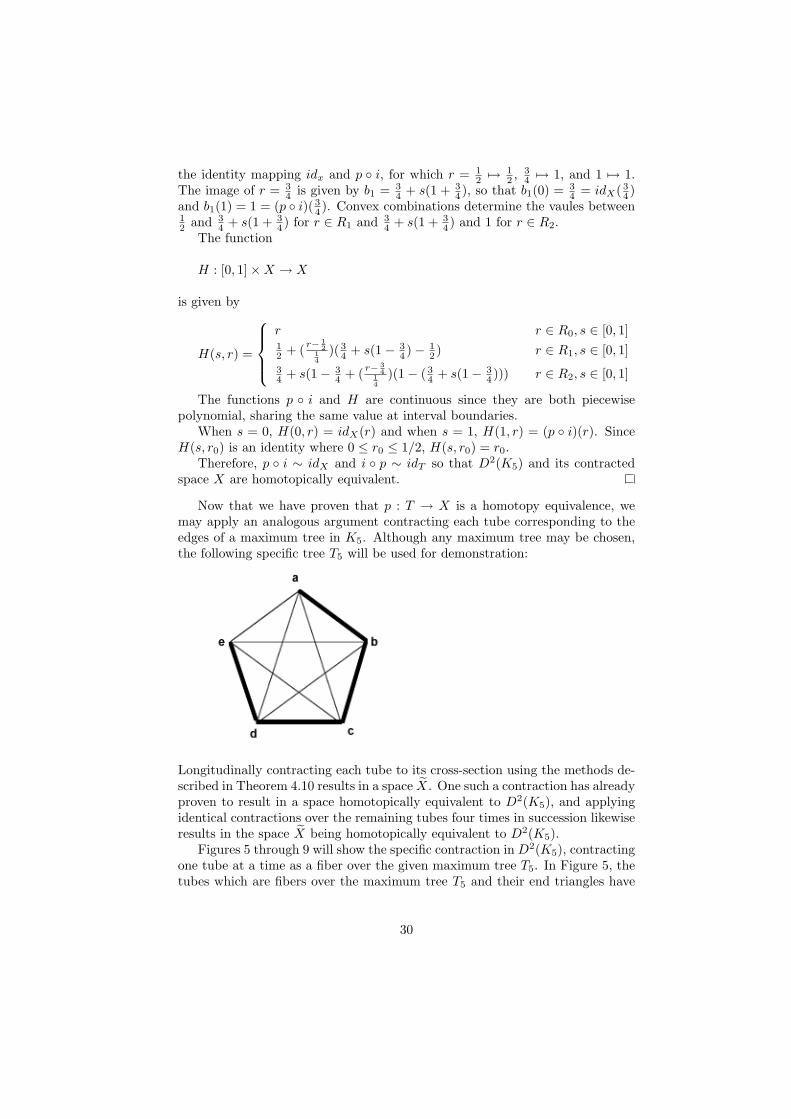
the identity mapping idx and p ◦ i, for which r = 12 7→ 1

2 , 34 7→ 1, and 1 7→ 1.

The image of r = 34 is given by b1 = 3

4 + s(1 + 34 ), so that b1(0) = 3

4 = idX( 34 )

and b1(1) = 1 = (p ◦ i)( 34 ). Convex combinations determine the vaules between

12 and 3

4 + s(1 + 34 ) for r ∈ R1 and 3

4 + s(1 + 34 ) and 1 for r ∈ R2.

The function

H : [0, 1] × X → X

is given by

H(s, r) =

r r ∈ R0, s ∈ [0, 1]12 + (

r− 1

2

1

4

)( 34 + s(1 − 3

4 ) − 12 ) r ∈ R1, s ∈ [0, 1]

34 + s(1 − 3

4 + (r− 3

4

1

4

)(1 − ( 34 + s(1 − 3

4 ))) r ∈ R2, s ∈ [0, 1]

The functions p ◦ i and H are continuous since they are both piecewisepolynomial, sharing the same value at interval boundaries.

When s = 0, H(0, r) = idX(r) and when s = 1, H(1, r) = (p ◦ i)(r). SinceH(s, r0) is an identity where 0 ≤ r0 ≤ 1/2, H(s, r0) = r0.

Therefore, p ◦ i ∼ idX and i ◦ p ∼ idT so that D2(K5) and its contractedspace X are homotopically equivalent.

Now that we have proven that p : T → X is a homotopy equivalence, wemay apply an analogous argument contracting each tube corresponding to theedges of a maximum tree in K5. Although any maximum tree may be chosen,the following specific tree T5 will be used for demonstration:

Longitudinally contracting each tube to its cross-section using the methods de-scribed in Theorem 4.10 results in a space X̃. One such a contraction has alreadyproven to result in a space homotopically equivalent to D2(K5), and applyingidentical contractions over the remaining tubes four times in succession likewiseresults in the space X̃ being homotopically equivalent to D2(K5).

Figures 5 through 9 will show the specific contraction in D2(K5), contractingone tube at a time as a fiber over the given maximum tree T5. In Figure 5, thetubes which are fibers over the maximum tree T5 and their end triangles have

30

been denoted by color. Points have been labeled with the position of Robot 1then the position of Robot 2, separated by a comma. As each tube is contracted,the labling of the first position is changed to the names of the contracted pointsin K5 separated by parenthesis. For example, in Figure 6, the tube which wasthe fiber of edge ab in K5 has been contracted, and the resulting cross-sectionis labeled by the points (ba), c, (ba), d and (ba), e.

4.4 Application of the Seifert-Van Kampen Theorem

After the contraction on the four tubes being the fibers of edges ab, bc, cd, andde, the space X̃ is composed of six remaining tubes. The end triangles of eachtube are loops in the space X̃ so that there are twelve such loops connected inpairs by six tubes. In Figure 10, these loops have been designated such that twoloops with the same shading are the mutual end triangles of a tube. It can alsobe confirmed that each edge of an end triangle is a shared edge with exactlyone other distinct end triangle.

Besides its two end triangles, each triangular tube contains three distincttube edges, each connecting a vertex on an end triangle to its correspondingvertex on the second end triangle. In X̃, these are represented as two tripleedges, a quadruple edge, and eight loops containing a single vertex each, to-taling eighteen edges, three for each of six tubes. It can be confirmed that thenumber of these edges at any given vertex is equal to the number of end trianglescontaining that particular vertex.

Our calcuation of the fundamental group of D2(K5) will be based on theSeifert-Van Kampen theorem, whose statement characterizes the fundamentalgroup of a space in terms of fundamental groups of subspaces. Before applyingthe theorem, we will have to do one more contraction to create a space homo-topically equivalent to X̃. This space decomposes into subspaces in such a waythat the Seifert-Van Kampen theorem implies that the fundamental group ofthe space is the free product of the fundamental group of the subspaces.

We wish to apply the Seifert-Van Kampen theorem to the contracted spaceX̃ in order to generate a new homotopically equivalent space and its fundamen-tal group. According to this theorem, after certain prerequisites are met, thefundamental group can be freely generated by the union of its components.

Definition 4.11. The space X is arcwise-connected if for any two points x andy in X there exists a continuous function f : [0, 1] → X such that f(0) = x andf(1) = y.

Theorem 4.12. (Seifert-Van Kampen)[9] Assume that U and V are arcwise-connected open subsets of X such thatX = U ∪ V and U ∩ V is nonempty and arcwise connected. Choose a basepointx0 ∈ U∩V for all fundamental groups under consideration. Let H be any group,and ρ1, ρ2, and ρ3 any three homomorphisms such that the following diagramis commutative:

31

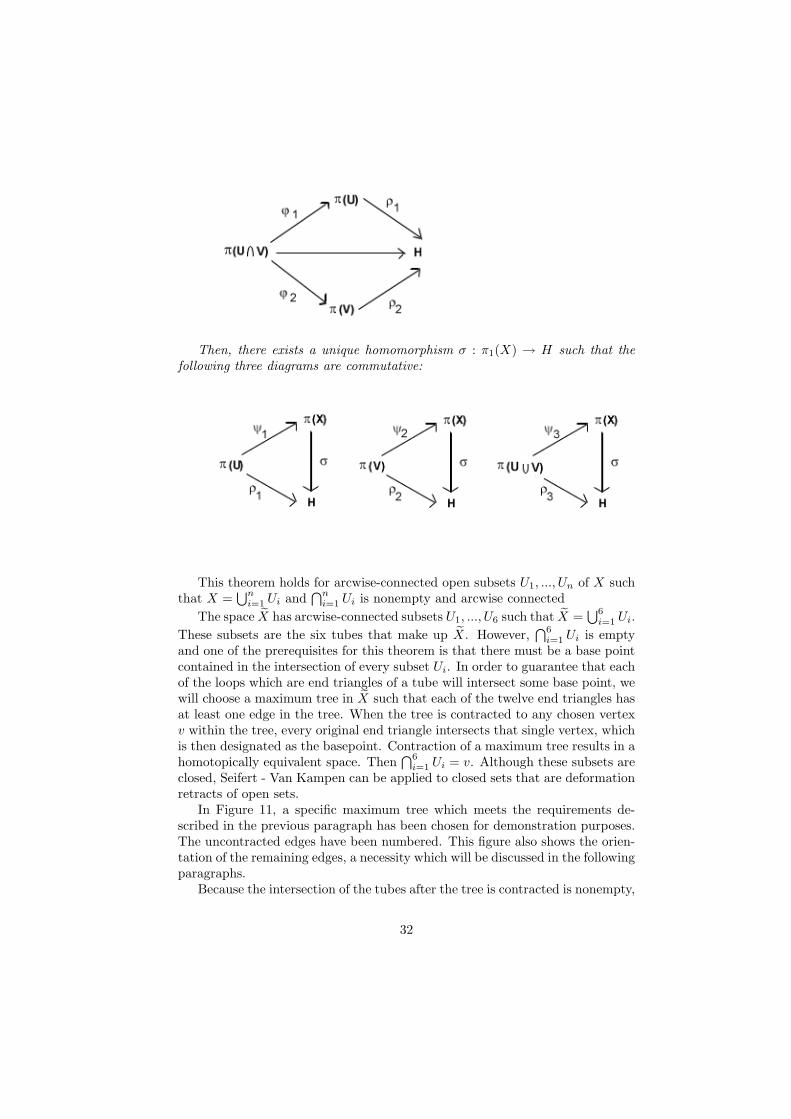
Then, there exists a unique homomorphism σ : π1(X) → H such that thefollowing three diagrams are commutative:

This theorem holds for arcwise-connected open subsets U1, ..., Un of X suchthat X =

⋃n

i=1 Ui and⋂n

i=1 Ui is nonempty and arcwise connected

The space X̃ has arcwise-connected subsets U1, ..., U6 such that X̃ =⋃6

i=1 Ui.

These subsets are the six tubes that make up X̃. However,⋂6

i=1 Ui is emptyand one of the prerequisites for this theorem is that there must be a base pointcontained in the intersection of every subset Ui. In order to guarantee that eachof the loops which are end triangles of a tube will intersect some base point, wewill choose a maximum tree in X̃ such that each of the twelve end triangles hasat least one edge in the tree. When the tree is contracted to any chosen vertexv within the tree, every original end triangle intersects that single vertex, whichis then designated as the basepoint. Contraction of a maximum tree results in ahomotopically equivalent space. Then

⋂6i=1 Ui = v. Although these subsets are

closed, Seifert - Van Kampen can be applied to closed sets that are deformationretracts of open sets.

In Figure 11, a specific maximum tree which meets the requirements de-scribed in the previous paragraph has been chosen for demonstration purposes.The uncontracted edges have been numbered. This figure also shows the orien-tation of the remaining edges, a necessity which will be discussed in the followingparagraphs.

Because the intersection of the tubes after the tree is contracted is nonempty,

32

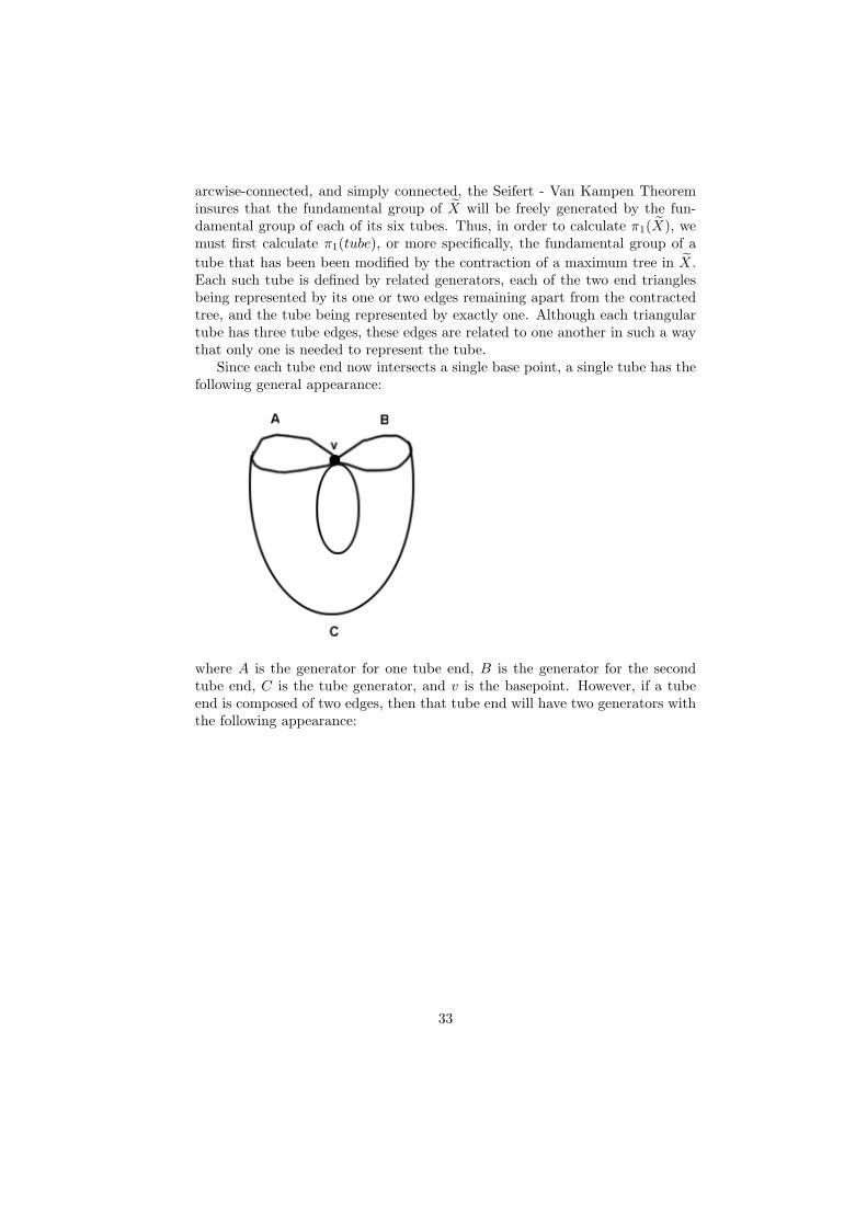
arcwise-connected, and simply connected, the Seifert - Van Kampen Theoreminsures that the fundamental group of X̃ will be freely generated by the fun-damental group of each of its six tubes. Thus, in order to calculate π1(X̃), wemust first calculate π1(tube), or more specifically, the fundamental group of a

tube that has been been modified by the contraction of a maximum tree in X̃.Each such tube is defined by related generators, each of the two end trianglesbeing represented by its one or two edges remaining apart from the contractedtree, and the tube being represented by exactly one. Although each triangulartube has three tube edges, these edges are related to one another in such a waythat only one is needed to represent the tube.

Since each tube end now intersects a single base point, a single tube has thefollowing general appearance:

where A is the generator for one tube end, B is the generator for the secondtube end, C is the tube generator, and v is the basepoint. However, if a tubeend is composed of two edges, then that tube end will have two generators withthe following appearance:

33

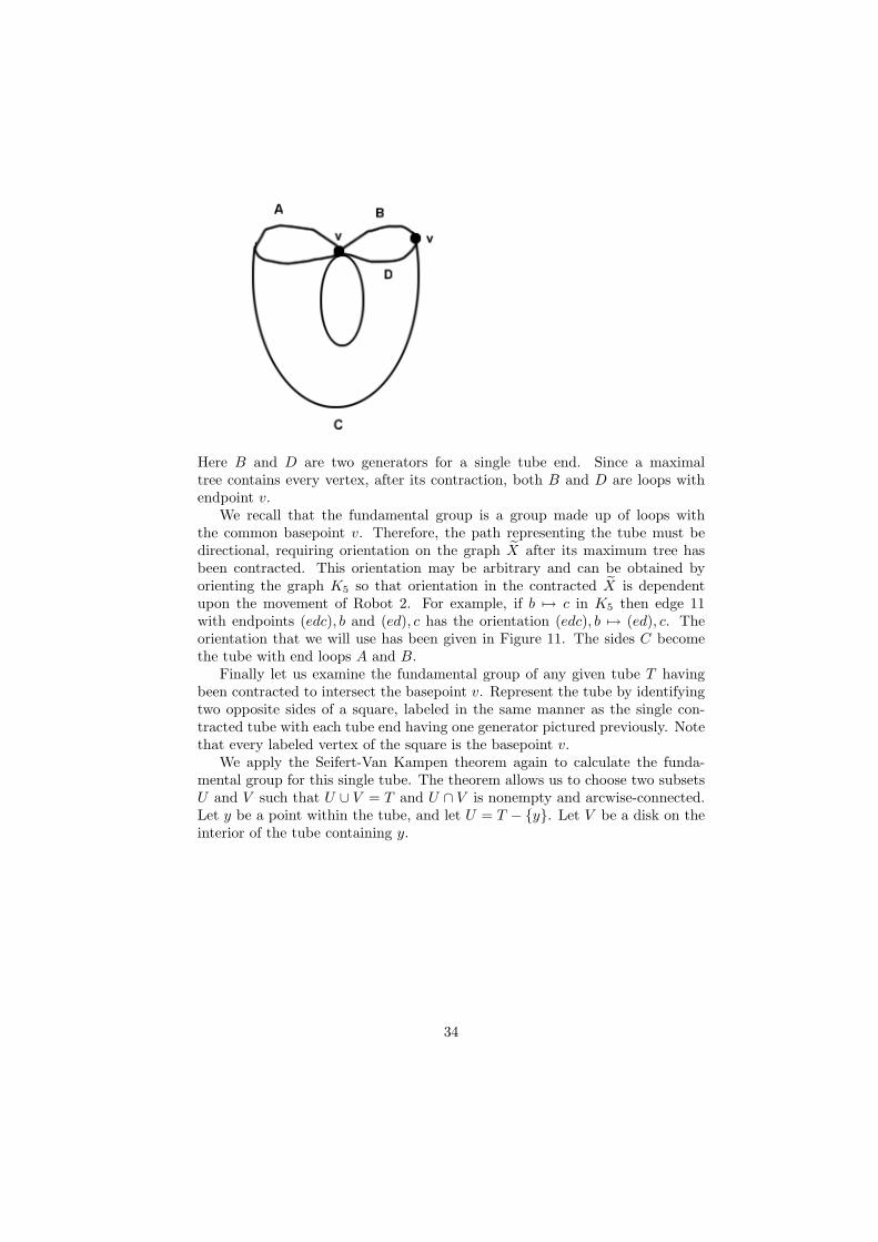
Here B and D are two generators for a single tube end. Since a maximaltree contains every vertex, after its contraction, both B and D are loops withendpoint v.

We recall that the fundamental group is a group made up of loops withthe common basepoint v. Therefore, the path representing the tube must bedirectional, requiring orientation on the graph X̃ after its maximum tree hasbeen contracted. This orientation may be arbitrary and can be obtained byorienting the graph K5 so that orientation in the contracted X̃ is dependentupon the movement of Robot 2. For example, if b 7→ c in K5 then edge 11with endpoints (edc), b and (ed), c has the orientation (edc), b 7→ (ed), c. Theorientation that we will use has been given in Figure 11. The sides C becomethe tube with end loops A and B.

Finally let us examine the fundamental group of any given tube T havingbeen contracted to intersect the basepoint v. Represent the tube by identifyingtwo opposite sides of a square, labeled in the same manner as the single con-tracted tube with each tube end having one generator pictured previously. Notethat every labeled vertex of the square is the basepoint v.

We apply the Seifert-Van Kampen theorem again to calculate the funda-mental group for this single tube. The theorem allows us to choose two subsetsU and V such that U ∪ V = T and U ∩ V is nonempty and arcwise-connected.Let y be a point within the tube, and let U = T − {y}. Let V be a disk on theinterior of the tube containing y.

34

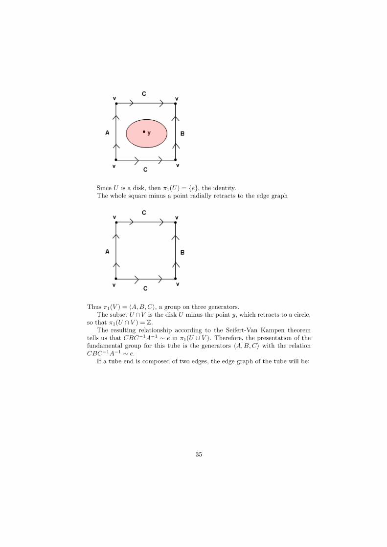
Since U is a disk, then π1(U) = {e}, the identity.The whole square minus a point radially retracts to the edge graph

Thus π1(V ) = 〈A,B,C〉, a group on three generators.The subset U ∩V is the disk U minus the point y, which retracts to a circle,

so that π1(U ∩ V ) = Z.The resulting relationship according to the Seifert-Van Kampen theorem

tells us that CBC−1A−1 ∼ e in π1(U ∪ V ). Therefore, the presentation of thefundamental group for this tube is the generators 〈A,B,C〉 with the relationCBC−1A−1 ∼ e.

If a tube end is composed of two edges, the edge graph of the tube will be:

35

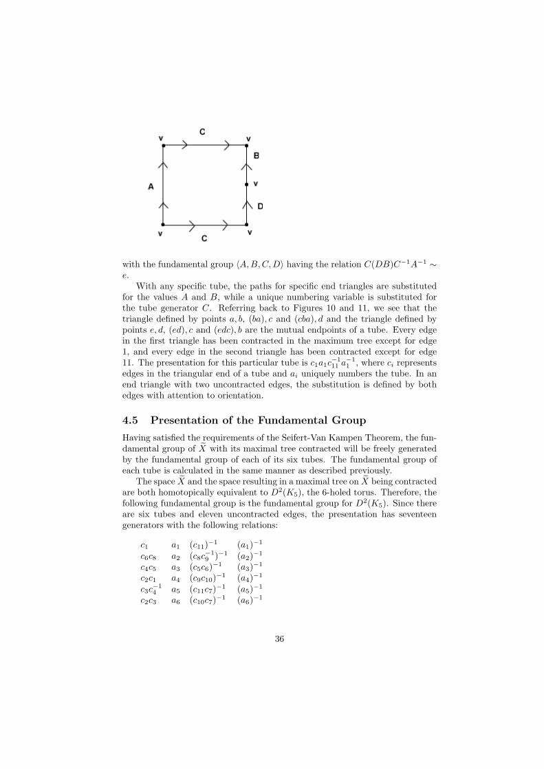
with the fundamental group 〈A,B,C,D〉 having the relation C(DB)C−1A−1 ∼e.

With any specific tube, the paths for specific end triangles are substitutedfor the values A and B, while a unique numbering variable is substituted forthe tube generator C. Referring back to Figures 10 and 11, we see that thetriangle defined by points a, b, (ba), c and (cba), d and the triangle defined bypoints e, d, (ed), c and (edc), b are the mutual endpoints of a tube. Every edgein the first triangle has been contracted in the maximum tree except for edge1, and every edge in the second triangle has been contracted except for edge11. The presentation for this particular tube is c1a1c

−111 a−1

1 , where ci representsedges in the triangular end of a tube and ai uniquely numbers the tube. In anend triangle with two uncontracted edges, the substitution is defined by bothedges with attention to orientation.

4.5 Presentation of the Fundamental Group

Having satisfied the requirements of the Seifert-Van Kampen Theorem, the fun-damental group of X̃ with its maximal tree contracted will be freely generatedby the fundamental group of each of its six tubes. The fundamental group ofeach tube is calculated in the same manner as described previously.

The space X̃ and the space resulting in a maximal tree on X̃ being contractedare both homotopically equivalent to D2(K5), the 6-holed torus. Therefore, thefollowing fundamental group is the fundamental group for D2(K5). Since thereare six tubes and eleven uncontracted edges, the presentation has seventeengenerators with the following relations:

c1 a1 (c11)−1 (a1)

−1

c6c8 a2 (c8c−19 )−1 (a2)

−1

c4c5 a3 (c5c6)−1 (a3)

−1

c2c1 a4 (c9c10)−1 (a4)

−1

c3c−14 a5 (c11c7)

−1 (a5)−1

c2c3 a6 (c10c7)−1 (a6)

−1

36

The cis represent uncontracted edges in the triangular end of a tube and theais uniquely number each tube.

We recall that the braid group associated with the configuration of a pairof points in the plane is isomorphic to Z. The fundamental group of a graphconfiguration space generated by two robots is a much more complex space.Some difficulties arise when trying to compare it to the standard presentationof the fundamental group of the 6-holed torus, although we know that bothpresentations must give isomorphic groups.

The standard presentation for the 6-holed torus, to which D2(K5) is isomor-phic, consists of the set of generators {α1, β1, ..., αn, βn} and the single relationΠi=1

n [αi, βi], where Πi=1n [αi, βi] denotes the commutator αiβiα

−1i β−1

i .“Any group admits many different presentations, which may look quite dif-

ferent. Conversely, given two presentations... it is often nearly impossible todetermine whether or not the two groups thus defined are isomorphic” [9]. Soalthough we cannot determine whether the given presentation is isomorphicto the standard presentation, the standard presentation has twelve generators.Although abelianizing our presentation will not prove isomorphism, a total oftwelve generators after abelianization will show that our presentation may becorrect, while any other number will show a definite mistake in our calculations.Each of the tube generators a1, a2, ..., a6 is independent, so the relations betweenthe end triangle generators must cancel out some of these generators.

We find that every generator ci is a product of the six generators c1, c5, c7,c8, c9, and c10.

There are five remaining generators, but each may be re-expressed in termsof the above six. The equations containing these five are all tautologies.

Thus the abelianized fundamental group is freely generated by twelve gen-erators, six tube generators a1, a2, ..., a6 and six edge generators c1, c5, c7, c8, c9

and c10. This confirms that the abelianized fundamental group of D2(K5) hasthe same number of generators as the standard presentation for the fundamentalgroup of the 6-holed torus.

The relationship to braid groups and the study of special structures are justa few aspects of topology in graph configuration spaces. There are numerousremaining questions about these spaces, in the topics we have covered as wellother areas of topology. Graph configuration spaces may be used in a practicalphysical setting as with the robots in a factory, or in almost purely theoreticalbranches of mathematics. Hopefully work in understanding graph configura-tion spaces and their fundamental groups will continue until they are as wellunderstood as the braid groups that they resemble.

37

Bibliography

[1] Abrams, A. D. (2000). Configuration spaces and braid groups of graphs,Ph.D thesis, University of California, Berkeley: 67 leaves.

[2] Fernandes, P. (2003). Topology of Graph Configuration Spaces, VirginiaTech. http://www.math.vt.edu/people/linnell/Ugresearch/fernandes.pdf:36.

[3] Abrams, A. D. and R. Ghrist (2002). “Finding topology in a factory: con-figuration spaces.” American Mathematical Monthly 109(2): 140-150.

[4] Ghrist, R. and D. Koditschek (2002). “Safe, cooperative robot dynamicson graphs”. SIAM J. Control and Optimization 40(5): 1556-1575.

[5] Koditschek, D. and E. Rimon (1990). “Robot navigation functions on man-ifolds with boundary”. Adv. in Appl. Math 11: 412-442.

[6] Ghrist, R. (2001). “Configuration spaces and braid groups on graphs inrobotics:”. Braids, Links, and Mapping Class Groups: the Proceedings ofJoan Birman’s 70th Birthday, AMS/IP Studies in Mathematics, volume 24:29-40.

[7] Crisp, J. and Burt Wiest (2004). “Embeddings of graph braid and sur-face groups in right-angled Artin groups and braid groups”. Algebraic andGeometric Topology 4: 439-472.

[8] West, D. B. (2001). Introduction to graph theory. Upper Saddle River, N.J.,Prentice Hall.

[9] Massey, W. S. (1977). Algebraic topology, an introduction. New York,Springer-Verlag.

[10] Fulton, W. (1995). Algebraic topology : a first course. New York, Springer-Verlag.

38

List of Figures

1 Fibration over the point a in K5 . . . . . . . . . . . . . . . . . . 402 Fibration over the edge ab in K5 . . . . . . . . . . . . . . . . . . 403 The mapping p : T → X . . . . . . . . . . . . . . . . . . . . . . . 414 The mapping i : X → T . . . . . . . . . . . . . . . . . . . . . . . 425 D2(K5) . . . . . . . . . . . . . . . . . . . . . . . . . . . . . . . . 436 Contraction of the fibration over edge ab in K5 . . . . . . . . . . 447 Contraction of the fibration over edge bc in K5 . . . . . . . . . . 458 Contraction of the fibration over edge cd in K5 . . . . . . . . . . 469 Contraction of the fibration over edge de in K5 . . . . . . . . . . 4710 Six triangular tubes with tube ends specified by shading . . . . . 4811 Maximum tree and orientation . . . . . . . . . . . . . . . . . . . 49

39

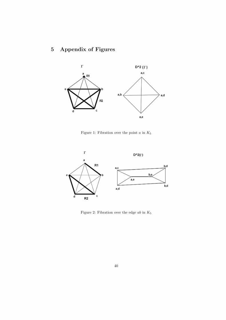
5 Appendix of Figures

Figure 1: Fibration over the point a in K5

Figure 2: Fibration over the edge ab in K5

40

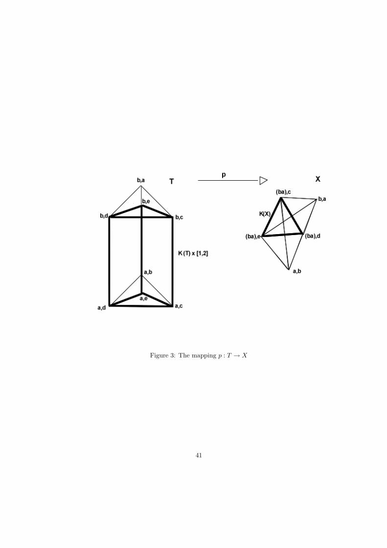
Figure 3: The mapping p : T → X

41

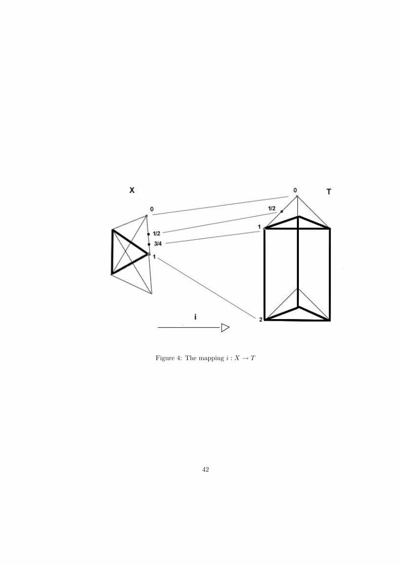
Figure 4: The mapping i : X → T

42

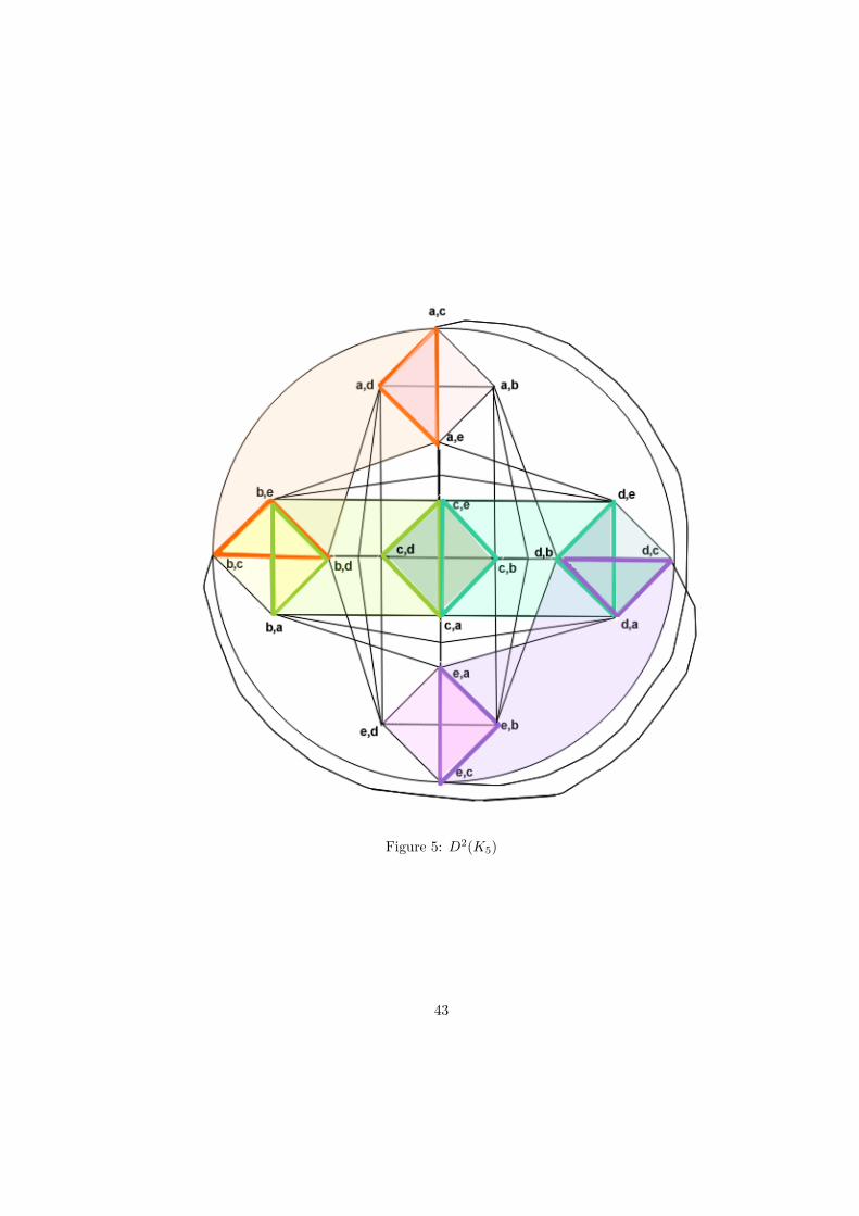
Figure 5: D2(K5)

43

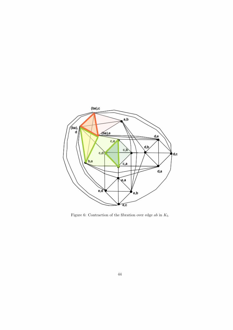
Figure 6: Contraction of the fibration over edge ab in K5

44

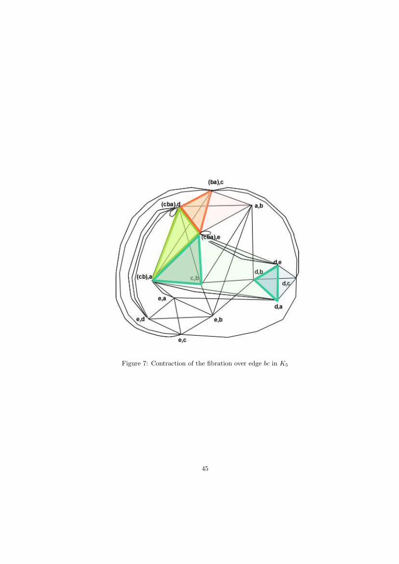
Figure 7: Contraction of the fibration over edge bc in K5

45

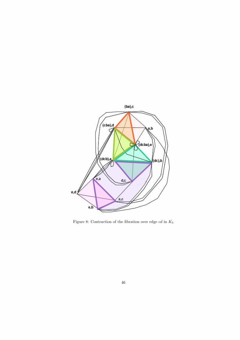
Figure 8: Contraction of the fibration over edge cd in K5

46

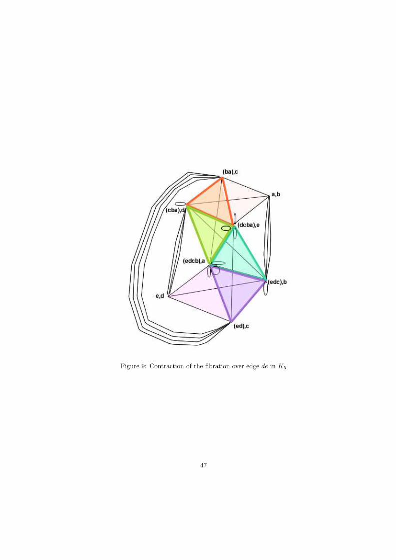
Figure 9: Contraction of the fibration over edge de in K5

47

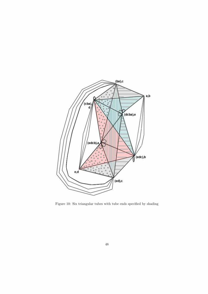
Figure 10: Six triangular tubes with tube ends specified by shading

48

Figure 11: Maximum tree and orientation

49