Two-dimensional laminar shock wave / boundary layer interaction

J.-Ch. Robinet(1), V. Daru(1,2) and Ch. Tenaud(2)

(1) SINUMEF Laboratory, ENSAM-PARIS151, Bd. de l’Hopital, PARIS 75013, France

(2) LIMSI-CNRSB.P. 133, 91403 ORSAY Cedex, France

robinet@paris.ensam.fr, daru@paris.ensam.fr, tenaud@limsi.fr

1. Introduction

Compressible flows involving a shock wave/boundary layer interaction (SWBLI) can be en-countered in a number of industrial applications (buffet, side load in over-extended nozzles, airinlet...). Moreover, for some configurations, low frequency unsteadiness can be originated inthese SWBLI, which can spoil the system or dramatically reduce the performances. The controlof such a flow with efficiency and a reasonable cost constitutes a major challenge for the nearfuture. In order to attain this objective, it is necessary to understand the physical mechanismresponsible for the appearance of unsteadiness. This implies the development of very accurateand low cost numerical methods for the simulation of such flows.

The aim of this paper is to evaluate the efficiency of different numerical methods, and alsoto quantify the effect of the grid and the boundary conditions, in the case of an oblique shockinteracting with a boundary layer developing along a plane wall. The flow configuration is similarto the one in [7] and [4], but here we increase the angle of the incident shock until unsteadinessappears. The study is limited to the two-dimensional case, and we will discuss the consequencesof this restriction.

2. Numerical methods

The numerical solution of our shock wave/laminar boundary-layer interaction problem isobtained by solving the 2D unsteady compressible Navier-Stokes equations written here in con-servative form:

wt +(

fE− fV

)

x+

(

gE− gV

)

y= 0, (1)

where w = (ρ, ρu, ρv, ρE)t is the state vector expressed in terms of the conservative variablesdensity, momentum and total energy, fE = fE(w), gE = gE(w) are the Euler fluxes, fV =fV (w,wx, wy), gV = g(w,wx, wy) stand for the viscous fluxes in the two space directions. System(1) is closed by assuming that the air satisfies the perfect gas equation with a constant specificheat ratio γ: p = (γ − 1)ρe, with p the pressure and e the internal energy; moreover the Prandtlnumber is also supposed to be constant and set equal to 0.72.For solving the Navier-Stokes equations, two different numerical schemes have been used.

2..1. AUSM+ scheme

System (1) is spaced-discretized on a cartesian grid using the following conservative scheme:

wt +

[

δx

(

fE − fV)]

ijk

(δxx)ijk+

[

δy

(

gE − gV)]

ijk

(δyy)ijk

= 0, (2)

where δp denotes the standard difference over a single cell in the pth space direction, fE, gE arethe numerical fluxes approximating the physical convective fluxes and fV , gV are the second-order centered approximations of the physical viscous fluxes.

1

The invicid numerical fluxes are computed using the AUSM + scheme developped by Liou andEdwards (1998) [1]. This scheme was retained over flux-vector splitting schemes such as VanLeer’s for its well-known greater accuracy when applied to viscous flow computations and wasalso preferred over flux-difference splitting schemes such as Roe’s for its reduced cost. Purelycentered methods were ruled out for the present highly compressible flow calculations becausethey would have required the balance of artificial viscosity parameters and / or discontinuitysensors. High-accuracy of the invicid numerical fluxes is ensured through the use of a third andfifth-order MUSCL reconstruction of the vector of primitive variables (ρ, u, v, p)t. Usually, thereconstruction process also involves the use of a slope limiter in order to avoid the appearance ofnumerical oscillations in the solution. The main effect of this limiting process is to bring downthe accuracy of the scheme to the first order in flow regions where it is active: in turn, thisreduction of accuracy can subtantially alter the flow prediction, so that unsteady phenomenamay no longer spontaneously appear. In the present study, the use of such limiter was not foundnecessary because enough natural dissipation is provided by the viscous terms to prevent theoccurrence of numerical oscillations.

A time-accurate approximation solution of system (1) is obtained using the following implicitlinear multi-step method:

T (wn+1, wn, wn−1) + R(wn+1) = 0, (3)

where R gathers the space-discretization operators described in the previous section and T isthe three-step approximation of wt at time level (n + 1) defined by:

T(

wn+1, wn)

= (1 + φ)

(

wn+1 − wn)

∆t− φ

(

wn − wn−1)

∆t= (wt)

n+1 + O (∆p) . (4)

Th choice of φ = 1/2 in formula (4) allows to reach second-order accuracy in time (p = 2). Adual time technique, promoted by Jameson (1991) [2] to compute compressible flows, is usedto solve at each physical time-step the implicit system R∗

(

wn+1)

= 0 where R∗

(

wn+1)

=T

(

wn+1, wn)

+ R(

wn+1)

. Actually, wn+1 is obtained as a steady solution of an evolutionproblem with respect to a dual or fictious time τ :

wτ + R∗(w) = 0. (5)

Solving (5) instead of (3) allows the use of much larger physical time-steps; however, in the mean-time, it also requires converging to a pseudo steady-state at each physical time-step. Therefore,the dual time approach is of interest only if system (5) can be efficiently solved. In the presentstudy, a matrix-free point-relaxation method allows to obtain a steady solution of system (5)after a few number of subiterations on the dual time; moreover this implicit treatment induces alow storage requirement which makes the treatment of the large number of grid points accessiblewith moderate computer configurations (see for instance Luo et al. (2001) [3] for more detailson this implicit technique).

2..2. OSMP7 scheme

The second scheme (named OSMP7) was recently developed in [6]. It is an upwind, seventhorder accurate in time and space (at least in the scalar case) explicit scheme. It is basedon a coupled time-space Lax-Wendroff type approach, and a Strang splitting is used in themultidimensional case. For solving the Navier-Stokes equations, the scheme is formally onlysecond order accurate due to the splitting. Nevertheless, the level of error of the scheme is verylow, and it has been shown to give very accurate results for several test cases, using coarsemeshes [6]. A monotonicity-preserving constraint is incorporated to the scheme, which is activeonly in the vicinity of steep gradients regions where it acts similarly to a TVD limiter. In sucha way, no numerical oscillations are generated in calculating discontinuities (shock waves for

2

instance). In smooth regions and in the vicinity of extrema of the solution, the monotonicity-preserving constraint is naturally satisfied implying that the limiting process is not activated,and the order of accuracy of the scheme can be preserved. This is a very important differencewith classical TVD schemes, for which accuracy degrades to first order near extrema with theeffect of clipping extrema.

3. Computational domain and boundary conditions

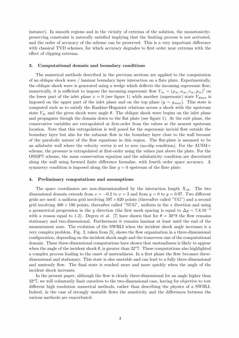
The numerical methods described in the previous sections are applied to the computationof an oblique shock wave / laminar boundary layer interaction on a flate plate. Experimentally,the oblique shock wave is generated using a wedge which deflects the incoming supersonic flow;numerically, it is sufficient to impose the incoming supersonic flow V∞ = (ρ∞, u∞, v∞, p∞)t onthe lower part of the inlet plane x = 0 (see figure 1) while another (supersonic) state Vdown isimposed on the upper part of the inlet plane and on the top plane (y = ymax). This state iscomputed such as to satisfy the Rankine-Hugoniot relations across a shock with the upstreamstate V∞ and the given shock wave angle θ. The oblique shock wave begins on the inlet planeand propagates though the domain down to the flat plate (see figure 1). At the exit plane, theconservative variables are extrapolated at first-order from the values at the nearest upstreamlocation. Note that this extrapolation is well posed for the supersonic invicid flow outside theboundary layer but also for the subsonic flow in the boundary layer close to the wall becauseof the parabolic nature of the flow equations in this region. The flat-plate is assumed to bean adiabatic wall where the velocity vector is set to zero (no-slip condition). For the AUSM+scheme, the pressure is extrapolated at first-order using the values just above the plate. For theOSMP7 scheme, the mass conservation equation and the adiabaticity condition are discretizedalong the wall using forward finite difference formulae, with fourth order space accuracy. Asymmetry condition is imposed along the line y = 0 upstream of the flate plate.

4. Preliminary computations and assumptions

The space coordinates are non-dimensionalized by the interaction length Xsh. The twodimensional domain extends from x = −0.2 to x = 2 and from y = 0 to y = 0.97. Two differentgrids are used: a uniform grid involving 597× 620 points (thereafter called ”UG”) and a secondgrid involving 400 × 180 points, thereafter called ”NUG”, uniform in the x direction and usinga geometrical progression in the y direction (the first mesh spacing is equal to ∆y = 7.8.10−5

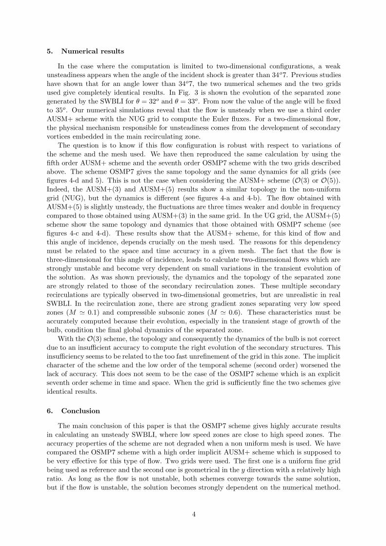
with a reason equal to 1.2). Degrez et al. [7] have shown that for θ = 30o8 the flow remainsstationary and two-dimensional. Furthermore it remains laminar at least until the end of themeasurement zone. The evolution of the SWBLI when the incident shock angle increases is avery complex problem. Fig. 2, taken from [5], shows the flow organization in a three-dimensionalconfiguration, depending on the incident shock angle and the transverse size of the computationaldomain. These three-dimensional computations have shown that unsteadiness is likely to appearwhen the angle of the incident shock θ, is greater than 32o7. These computations also highlighteda complex process leading to the onset of unsteadiness. In a first phase the flow becomes three-dimensional and stationary. This state is also unstable and can lead to a fully three-dimensionaland unsteady flow. The final state is reached more and more quickly when the angle of theincident shock increases.

In the present paper, although the flow is clearly three-dimensional for an angle higher than32o7, we will voluntarily limit ourselves to the two-dimensional case, having for objective to testdifferent high resolution numerical methods, rather than describing the physics of a SWBLI.Indeed, in the case of strongly unstable flows the sensitivity and the differences between thevarious methods are exacerbated.

3

5. Numerical results

In the case where the computation is limited to two-dimensional configurations, a weakunsteadiness appears when the angle of the incident shock is greater than 34o7. Previous studieshave shown that for an angle lower than 34o7, the two numerical schemes and the two gridsused give completely identical results. In Fig. 3 is shown the evolution of the separated zonegenerated by the SWBLI for θ = 32o and θ = 33o. From now the value of the angle will be fixedto 35o. Our numerical simulations reveal that the flow is unsteady when we use a third orderAUSM+ scheme with the NUG grid to compute the Euler fluxes. For a two-dimensional flow,the physical mechanism responsible for unsteadiness comes from the development of secondaryvortices embedded in the main recirculating zone.

The question is to know if this flow configuration is robust with respect to variations ofthe scheme and the mesh used. We have then reproduced the same calculation by using thefifth order AUSM+ scheme and the seventh order OSMP7 scheme with the two grids describedabove. The scheme OSMP7 gives the same topology and the same dynamics for all grids (seefigures 4-d and 5). This is not the case when considering the AUSM+ scheme (O(3) or O(5)).Indeed, the AUSM+(3) and AUSM+(5) results show a similar topology in the non-uniformgrid (NUG), but the dynamics is different (see figures 4-a and 4-b). The flow obtained withAUSM+(5) is slightly unsteady, the fluctuations are three times weaker and double in frequencycompared to those obtained using AUSM+(3) in the same grid. In the UG grid, the AUSM+(5)scheme show the same topology and dynamics that those obtained with OSMP7 scheme (seefigures 4-c and 4-d). These results show that the AUSM+ scheme, for this kind of flow andthis angle of incidence, depends crucially on the mesh used. The reasons for this dependencymust be related to the space and time accuracy in a given mesh. The fact that the flow isthree-dimensional for this angle of incidence, leads to calculate two-dimensional flows which arestrongly unstable and become very dependent on small variations in the transient evolution ofthe solution. As was shown previously, the dynamics and the topology of the separated zoneare strongly related to those of the secondary recirculation zones. These multiple secondaryrecirculations are typically observed in two-dimensional geometries, but are unrealistic in realSWBLI. In the recirculation zone, there are strong gradient zones separating very low speedzones (M ' 0.1) and compressible subsonic zones (M ' 0.6). These characteristics must beaccurately computed because their evolution, especially in the transient stage of growth of thebulb, condition the final global dynamics of the separated zone.

With the O(3) scheme, the topology and consequently the dynamics of the bulb is not correctdue to an insufficient accuracy to compute the right evolution of the secondary structures. Thisinsufficiency seems to be related to the too fast unrefinement of the grid in this zone. The implicitcharacter of the scheme and the low order of the temporal scheme (second order) worsened thelack of accuracy. This does not seem to be the case of the OSMP7 scheme which is an explicitseventh order scheme in time and space. When the grid is sufficiently fine the two schemes giveidentical results.

6. Conclusion

The main conclusion of this paper is that the OSMP7 scheme gives highly accurate resultsin calculating an unsteady SWBLI, where low speed zones are close to high speed zones. Theaccuracy properties of the scheme are not degraded when a non uniform mesh is used. We havecompared the OSMP7 scheme with a high order implicit AUSM+ scheme which is supposed tobe very effective for this type of flow. Two grids were used. The first one is a uniform fine gridbeing used as reference and the second one is geometrical in the y direction with a relatively highratio. As long as the flow is not unstable, both schemes converge towards the same solution,but if the flow is unstable, the solution becomes strongly dependent on the numerical method.

4

The AUSM+ scheme was shown to be less robust than the OSMP7 scheme, in particular inthe steep gradient zones where the grid is insufficiently refined. On the other hand the OSMP7scheme, thanks to a coupled time-space approach, makes it possible to preserve a good accuracyeven when the grid is insufficiently fine. However, the explicit character of the scheme makesthe convergence towards the solution very expensive.

References

[1] Edwards J., Liou M. S., “Low-diffusion flux-splitting methods for flows at all speeds”, AIAA

J., Vol. 36, pp. 1610-1617, 1998.

[2] Jameson A., “Time-dependent calculations using multigrid with applications to unsteadyflows past airfoils and wings”, AIAA Paper, 91-1596, 1991.

[3] Luo H., Baum J. D., Lohner R., “An accurate fast, matrix-free implicit method for comutingunsteady flows on unstructured grids”, Computers and Fluids, Vol. 30, pp. 137-159 (2001).

[4] Boin J.-Ph., Robinet J.-Ch., Corre Ch. “Interaction choc/couche limite laminaire : car-acteristiques instationnaires” Congres Francais de Mecanique, Nice, 1-5 September 2003.

[5] Boin J.-Ph., Robinet J.-Ch., Corre Ch., Deniau H. “3D steady and unsteady bifurcations ina laminar shock-wave / boundary layer interaction; a numerical study” Physics of Fluids,submitted Avril 2004.

[6] Daru V., Tenaud C. “High order one-step monotonicity-preserving schemes for unsteadycompressible flow calculations”, J. Comput. Phys., Vol. 193, pp. 563-594 (2004).

[7] Degrez G., Boccadoro C. H., Wendt J. F. “The interaction of an oblique shock wave with alaminar boundary layer revisited. An experimental and numerical study”, J. Fluid Mech.,Vol. 177, pp. 247-263 (1987).

Incident shock Leading edge shock

Expansion fan

Compressio

n waves

Compression waves

D

Xsh

R

M 8

������������������������������������������������������������������

Figure 1: Scheme of shock wave boundarylayer interaction with some notations used.

θ 32.532 3331.5

Lz

0.2

0.30.4

0.8

I II

III IV

I : steady 2D II : steady 3D III : unsteady 3D IV : unsteady 3D + 2D structure

Figure 2: Flow organization according to theincident shock angle the transverse size of thecomputation domain.

5

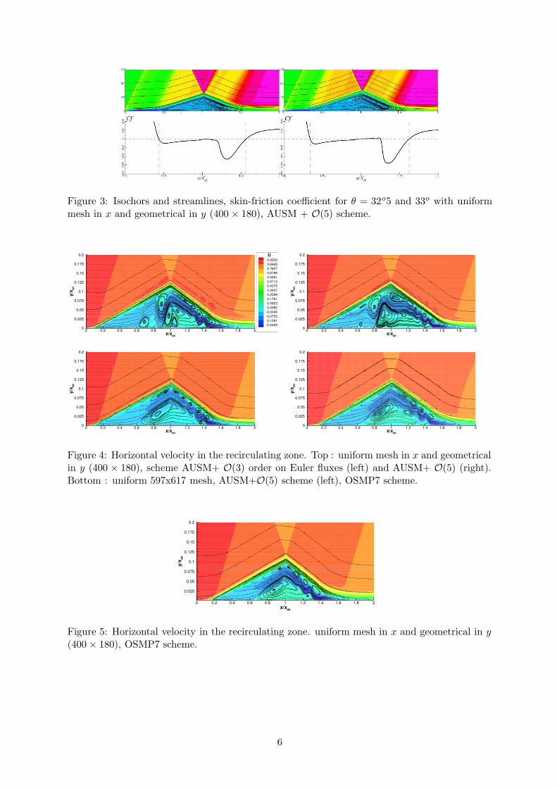
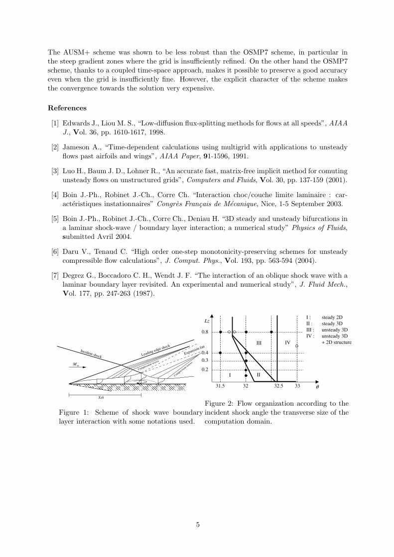
Figure 3: Isochors and streamlines, skin-friction coefficient for θ = 32o5 and 33o with uniformmesh in x and geometrical in y (400 × 180), AUSM + O(5) scheme.

x/xsh

y/x sh

0 0.2 0.4 0.6 0.8 1 1.2 1.4 1.6 1.8 20

0.025

0.05

0.075

0.1

0.125

0.15

0.175

0.20.93030.84650.76270.67890.59510.51130.42750.34370.25990.17610.09230.0085

-0.0046-0.0753-0.1591-0.2429

U

x/xsh

y/x sh

0 0.2 0.4 0.6 0.8 1 1.2 1.4 1.6 1.8 20

0.025

0.05

0.075

0.1

0.125

0.15

0.175

0.2

x/xsh

y/x sh

0 0.2 0.4 0.6 0.8 1 1.2 1.4 1.6 1.8 20

0.025

0.05

0.075

0.1

0.125

0.15

0.175

0.2

x/xsh

y/x sh

0 0.2 0.4 0.6 0.8 1 1.2 1.4 1.6 1.8 20

0.025

0.05

0.075

0.1

0.125

0.15

0.175

0.2

Figure 4: Horizontal velocity in the recirculating zone. Top : uniform mesh in x and geometricalin y (400 × 180), scheme AUSM+ O(3) order on Euler fluxes (left) and AUSM+ O(5) (right).Bottom : uniform 597x617 mesh, AUSM+O(5) scheme (left), OSMP7 scheme.

x/xsh

y/x sh

0 0.2 0.4 0.6 0.8 1 1.2 1.4 1.6 1.8 2

0.025

0.05

0.075

0.1

0.125

0.15

0.175

0.2

Figure 5: Horizontal velocity in the recirculating zone. uniform mesh in x and geometrical in y(400 × 180), OSMP7 scheme.

6