Embed Size (px)
Citation preview

1Icbrfs
wacptsvt
ttapailbi
t
3680 J. Opt. Soc. Am. A/Vol. 24, No. 12 /December 2007 Albert C. Fannjiang
Two-frequency radiative transfer: Maxwellequations in random dielectrics
Albert C. Fannjiang*
Department of Mathematics, University of California, Davis, Davis, California 95616-8633*[email protected]
Received July 6, 2007; accepted September 11, 2007;posted October 1, 2007 (Doc. ID 84859); published November 8, 2007
The paper addresses the space-frequency correlations of electromagnetic waves in general random, bianisotro-pic media whose constitutive tensors are complex Hermitian matrices. The two-frequency Wigner distribution(2f-WD) for polarized waves is introduced to describe the space-frequency correlations, and the closed formWigner–Moyal equation is derived from the Maxwell equations. Two-frequency radiative transfer (2f-RT) equa-tions are then derived from the Wigner–Moyal equation by using the multiple-scale expansion. For the sim-plest isotropic medium, the result coincides with Chandrasekhar’s transfer equation. In birefringent media,the 2f-RT equations take the scalar form due to the absence of depolarization. A number of birefringent mediasuch as chiral, uniaxial, and gyrotropic media are examined. For the unpolarized wave in an isotropic mediumthe 2f-RT equations reduces to the 2f-RT equation previously derived in part I of this research [J. Opt. Soc. Am.A 24, 2248 (2007)]. A similar Fokker–Planck-type equation is derived from the scalar 2f-RT equation for thebirefringent media. © 2007 Optical Society of America
OCIS codes: 030.5620, 290.4210.
tm=p−
�
wHmr
�
wtcoci[ft
. INTRODUCTIONn part I [1] of the series we studied the space-frequencyorrelation for scalar waves in random media as governedy the Helmholtz equation with a randomly fluctuatingefractive index. To this end, we introduced the two-requency Wigner distribution (2f-WD), which in the un-caled form is
W�x,p;�1,�2� =1
�2��3 � e−ip†yU1� x
�1+
y
2�1�
�U2*� x
�2−
y
2�2�dy,
here U1 and U2 are the wave fields at frequencies �1nd �2, respectively. Throughout, † denotes the Hermitianonjugation of vectors or matrices and * denotes the com-lex conjugation. The important characteristic of defini-ion (1) is that the spatial argument of each wave field iscaled in proportion to the respective wavelength. Theariables x are the so-called size parameter in scatteringheory when the phase velocity is unity [2].
In the weak-coupling (disorder) regime we derived thewo-frequency radiative transfer (2f-RT) equation for thewo-frequency Wigner distribution. We considered severalpproximations, notably the geometrical optics andaraxial approximations. Based on the dimensionalnalysis of these asymptotic equations, we obtained scal-ng behavior of the coherence bandwidth and coherenceength. We also obtained the space-frequency correlationelow the transport mean free path by analytically solv-ng one of the paraxial 2f-RT equations.
The main advantage of the 2f-RT theory over the tradi-ional equal-time RT theory is that it describes not just
1084-7529/07/123680-11/$15.00 © 2
he energy transport but also the two space–time pointutual coherence in the following way. Let u�tj ,xj� , j1,2 be the time-dependent wave field at two space–timeoints �tj ,xj� , j=1,2. Let x= ��1x1+�2x2� /2 and y=�1x1�2x2. Then we have
u�t1,x1�u*�t2,x2��
=� ei��2t2−�1t1��U1�x1�U2*�x2��d�1d�2
=� eip†ye−i��te−i���W�x,p;� + ��/2,� − ��/2��
�d� d��dp, �1�
ith t= �t1+ t2� /2 ,�= t1− t2 ,�= ��1+�2� /2 ,��=�1−�2.ere and below �·� is the ensemble averaging w.r.t. theedium fluctuations. In comparison, the single-time cor-
elation gives rise to the expression
u�t,x1�u†�t,x2��
=� eip†ye−i��t�� �W�x,p;� + ��/2,� − ��/2��d��d��dp,
hich, through spectral decomposition, determines onlyhe central-frequency-integrated 2f-WD. For a statisti-ally stationary signal, Eq. (1) would be a function of �nly. In this case different frequency components are un-orrelated and consequently only the equal-frequency WDs necessary to describe the two-space–time correlation3]. For statistically nonstationary signals the two-requency cross correlation is needed to characterize thewo-space–time correlation.
007 Optical Society of America

ctwtttmssiw
2lnmWtwbtirtavtrlgfatsrar
2WIpeif
wi
wat�
i
lifolpKsetacima
pdtfdoa
f
W
w�ataflantmor
t
Iuc
a
p
w
w
Albert C. Fannjiang Vol. 24, No. 12 /December 2007 /J. Opt. Soc. Am. A 3681
The 2f-RT theory developed in part I has enabled pre-ise estimation of important physical quantities such ashe coherence length and the coherence bandwidth [1],hich are medium characteristics relevant to communica-
ions and imaging in disordered media [4,5]. In particular,he two-frequency formulation is an indispensable tool forhe statistical stability analysis of the time-reversal com-unication scheme with broadband signals in multiple-
cattering media (see [4], where a 2f-RT equation and itsolution play a key role). The 2f-RT theory developed heres expected to extend these results to the case of polarizedaves.The organization of this paper is as follows. In Sectionand Appendix A, we develop the two-frequency formu-
ation of the Maxwell equations for a general heteroge-eous dielectric in terms of 2f-WD. In Section 3, we for-ulate the weak-coupling scaling limit for two-frequencyigner–Moyal equation. In Section 4 we develop the mul-
iscale expansion to find an approximate solution in theeak-coupling regime. In Section 5 and Appendix B,ased on a solvability condition we give an explicit form tohe 2f-RT equations for general bianisotropic media andn Subsection 5.A we derive a scalar 2f-RT equation for bi-efringent media. In Subsection 6.A, we consider the iso-ropic medium and show that the general 2f-RT equationsfter a change of variable reduces to the two-frequencyersion of Chandrasekhar’s transfer equation. In Subsec-ions 6.B–6.D, we examine three birefringent media: chi-al, uniaxial, and gyrotropic media. In Section 7, we ana-yze the unpolarized wave in the isotropic medium in theeometrical optics regime and show that the two-requency version of Chandrasekhar’s equation reduces toFokker–Planck-type equation rigorously derivable from
he geometrical optics of the scalar wave [6]. We derive aimilar equation from the scalar 2f-RT equation for the bi-efringent media. We conclude the paper in Section 8 withbrief discussion on expressing the two-space–time cor-
elation in terms of solutions of the 2f-RT equations.
. MAXWELL EQUATIONS ANDIGNER–MOYAL EQUATIONS
n this paper, we consider the electromagnetic waveropagation in a heterogeneous, lossless, bianisotropic di-lectric medium. We assume that the scattering mediums free of charges and currents and start with the source-ree Maxwell equations in the frequency domain,
− i�K�E
H + � 0 − ��
�� 0 �E
H = 0, �2�
here K is, by the assumption of losslessness, a Hermit-an matrix [7],
K = � K� K�
K�† K� , �3�
ith the permittivity and permeability tensors K� ,K�,nd the magnetoelectric tensor K� [8]. The Hermitian ma-rix K is assumed to be always invertible. Here and below,� denotes the curl operator.In an isotropic dielectric, K�=�I, K�=�I, K�=0. In a bi-
sotropic dielectric, K� as well as K� ,K� are nonzero sca-
ars. A reciprocal chiral medium is biisotropic with purelymaginary K�= i�. The appearance of nonzero K� arisesrom the so called magnetoelectric effect [9]. Crystals areften naturally anisotropic, and in some media (such asiquid crystals) it is possible to induce anisotropy by ap-lying, e.g., an external electric field. In crystal optics,� ,K� are real, symmetric matrices and K�=0 [10]. In re-
ponse to a magnetic field, some materials can have a di-lectric tensor that is complex-Hermitian; this is calledhe gyrotropic effect. In general, a magnetoelectric, bi-nisotropic medium has a constitutive tensor (3) withomplex Hermitian K� ,K� and a complex matrix K� sat-sfying the Post constraint [11]. It has been shown that a
oving medium, even isotropic, must be treated as bi-nisotropic [9,12].In general, K is a function of the frequency � (for dis-
ersive media), but it turns out that if the frequency-ependence of K is sufficiently smooth, the 2f-RT equa-ions derived in the present framework have the sameorm as for nondispersive media; the frequency depen-ence would enter the coefficients of the equations in thebvious way [1]. For simplicity of presentation we shallssume that the medium is nondispersive.Writing the total field U= �E ,H�, we introduce the two-
requency matrix-valued Wigner distribution,
�x,p;�1,�2�
=1
�2��3 � e−ip†yU1� x
�1+
y
2�1�U2
†� x
�2−
y
2�2�dy, �4�
here U1 and U2 are the total fields at frequencies �1 and2, respectively. From the definition we see that the vari-bles x and p−1 have the dimension of length/time. Al-hough the scaling factors in the arguments of U1 and U2re not required for the development of the 2f-RT theoryor the first-order (Maxwell) equations, they are particu-arly useful in the case of the second-order (Helmholtznd paraxial wave) equations. For consistency and conti-uity of presentation (see Section 7) we work with defini-ion (4) in the present paper. For an alternative develop-ent of the 2f-RT theory for Maxwell’s equations in terms
f the 2f-WD without the scaling factors, we refer theeader to [13].
First note the symmetry of the Wigner distribution ma-rix:
W†�x,p;�1,�2� = W�x,p;�2,�1�. �5�
n other words, the right-hand side of Eq. (4) is invariantnder the simultaneous transformations of Hermitianonjugation † and frequency exchange �1↔�2.
In what follows we shall omit writing the arguments ofny fields if there is no risk of confusion.We put Eq. (5) in the form of a general symmetric hy-
erbolic system [14,15],
− i�KU + Rl�xlU = 0, �6�
here the symmetric matrices Rj are given by
Rj = � 0 Tj
− Tj 0 ,
ith

Tm
cvjvvt
o
wa
Ht
F
3Aw
wbtsmi
wrbsm
Wts
srsta
r=
T
s
F
llfinTw
w(
3682 J. Opt. Soc. Am. A/Vol. 24, No. 12 /December 2007 Albert C. Fannjiang
T1 = 0 0 0
0 0 − 1
0 1 0�, T2 =
0 0 1
0 0 0
− 1 0 0�, T3 =
0 − 1 0
1 0 0
0 0 0� .
he matrices iTj , j=1,2,3 are related to the photon spinatrices [16].Throughout this paper the dot notation, “·”, is used ex-
lusively for the directional derivative as in p ·�=pj�xj. All
ectors are treated as matrices, and the scalar product isust the matrix multiplication between row and columnectors. All vectors are taken to be, by default, columnectors, unless explicitly transposed. Einstein’s summa-ion is applied to all english indices.
Applying the operator Rj� /�xj to W and using Eq. (6) webtain
Rj
�
�xjW = − 2ipjRjW + 2i� eiq†x/�1K�q�W�x,p −
q
2�1�dq,
�7�
hose derivation is given in Appendix A. From Eqs. (7)nd (5) we also have
�
�xjWRj
† = 2iWpjRj − 2i�W�x,p +q
2�2�K�q�eiq†x/�2dq.
�8�
ere and below, K stands for the Fourier transform (spec-ral density) of K as in
K�x� =� eix†qK�q�dq.
or a Hermitian K we have K�p�=K†�−p�, ∀p.
. WEAK-COUPLING LIMITs in part I [1] we consider the weak-coupling regimeith the tensor
K�x� = K0�I + ��V�x/���, � � 1, �9�
here the Hermitian matrix K0 represents the uniformackground medium and ��V represents the relative fluc-uations of the permittivity–permeability tensor. Themall parameter l describes the ratio of the scale of theedium fluctuation to the propagation distance. In an
sotropic dielectric,
K0 = ��0I3 0
0 �0I3, V = ��I3 0
0 �I3 ,
here � and � are the electric and magnetic susceptibility,espectively. In general K0 is a Hermitian matrix, and itslocks, as in Eq. (3), are denoted by K0
� ,K0� ,K0
� ,K0�†, re-
pectively. To preserve the Hermiticity of K and K0 theatrix V must satisfy
V†K0 = K0V. �10�
e shall assume below that K0 is either positive or nega-ive definite. Otherwise, the materials would be lossyince the refractive index is not real valued if K is not
0ign definite. A negative-definite K0 gives rise to negativeefractive index, which is a hot topic in metamaterial re-earch [17–19]. To fix the idea, let us take K0 to be posi-ive definite. With minor notational change, our methodpplies equally well to the negative definite case.We assume that V= Vij� is a statistically homogeneous
andom field with the spectral density tensors � ijmn�, �= ijmn� such that
�Vij�x�Vmn* �y�� =� eik†�x−y�ijmn�k�dk �11�
�Vij�x�Vmn�y�� =� eik†�x−y�ijmn�k�dk. �12�
his implies the following relations:
�Vij�p�Vmn* �q�� = ijmn�p���p − q�, �13�
�Vij�p�Vmn�q�� = ijmn�p���p + q�. �14�
In the case of real-valued V, �=�. The spectral den-ity tensors have the basic symmetry
ijmn* �p� = mnij�p�, �15�
ijmn�− p� = mnij�p�, �16�
urthermore, Eq. (10) implies that
K0,ijmnjl�p� = K0,lj* mnji�p�, �17�
K0,ijmnjl�p� = K0,lj* mnji�p�. �18�
As in part I, we consider the regime where the wave-engths are of the same order of magnitude as the corre-ation length of the medium fluctuations by rescaling therequencies �j= �j /� , j=1,2. This choice of frequency scal-ng results in strong scattering by the medium heteroge-eities. For ease of notation, we drop the tilde in �j below.o capture the high-frequency behavior of the wave field,e redefine the 2f-WD as
W�x,p� =1
�2��3 � e−ip†yU1� x
�1+
�y
2�1�U2
†� x
�2−
�y
2�2�dy.
�19�
We also assume that �1 ,�2→� as �→0 such that
�2 − �1
��= � �20�
ith a fixed constant �. The governing equations for Eq.19) become
Rj
�
�xjW = −
2i
�pjRjW +
2i
�K0W
+2i
��� eiq†x/�1K0V�q�W�p −
q
2�1�dq,
�21�

wcft
T2(ma
t
−
not
4Tf
Tsc
tm
AT
=fit
[tvkKdtsmdte
vaw
SKItc
Tt
dmtaHc
(
w
Albert C. Fannjiang Vol. 24, No. 12 /December 2007 /J. Opt. Soc. Am. A 3683
�
�xjWRj =
2i
�WpjRj −
2i
�WK0
−2i
���W�p −
q
2�2�V†�q�K0e−iq†x/�2dq,
�22�
here x=x /� is the fast spatial variable. In order to can-el the background effect, we multiply Eq. (21) by K0
−1
rom the left and Eq. (22) by K0−1 from the right and add
hem to obtain the symmetrical form
K0−1Rj
�
�xjW +
�
�xjWRjK0
−1 +2i
� K0
−1pjRjW − WpjRjK0−1�
=2i
��� �eiq†x/�1V�q�W�p −
q
2�1�
− W�p −q
2�2�V†�q�e−iq†x/�2dq. �23�
his is the equation that we shall work with to derive thef-RT equations employing the multiscale expansionMSE) [1,15]. Note that Eq. (23) is invariant under the si-
ultaneous transformations of Hermitian conjugation †
nd frequency exchange �1↔�2.If, instead of adding the two equations, we subtract
hem, then we obtain the antisymmetric form
4i
�W + K0
−1Rj
�
�xjW −
�
�xjWRjK0
−1 +2i
� K0
−1pjRjW
+ WpjRjK0−1�
=2i
��� �eiq†x/�1V�q�W�p −
q
2�1�
+ W�p −q
2�2�V†�q�e−iq†x/�2dq. �24�
Equation (24) requires a different treatment and willot be pursued here. However, the leading order �−1 termsf Eq. (24) impose a constraint, which will be discussed inhe Conclusion.
. MULTISCALE EXPANSIONhe key point of MSE is to separate the fast variable x
rom the slow variable x and make the substitution
Rj�xjW → Rj
�
�xjW + �−1Rj
�
�xjW,
�xjWRj →
�
�xjWRj + �−1
�
�xjWRj.
he idea is that for sufficiently small � the two widelyeparated scales, represented by x and x respectively, be-ome mathematically (but not physically) independent.
We posit the expansion W=W+��W1+�W2+¯, substi-ute it into Eq. (23), and equate terms of same order ofagnitude.
. Leading Termhe �−1 terms yield
K0−1Rj
�
�xjW +
�
�xjWRjK0
−1 + 2i K0−1pjRjW − WpjRjK0
−1� = 0.
�25�
We hypothesize that the leading order term WW�x ,p� is independent of the fast variable x. Thus therst two terms of Eq. (25) vanish so the equation reduceso
K0−1pjRjW − WpjRjK0
−1 = 0. �26�
Equation (26) arises also in the equal-time RT theory15] and can be solved as follows. For a positive (or nega-ive) definite K0, consider the eigenvalues � �� and eigen-ectors �e�,�� of the matrix K0
−1pjRj, where the index �eeps track of the multiplicity and hence depends on �. As
0−1pjRj is Hermitian with respect to the scalar productefined by a†K0b , ∀a ,b�C6, the eigenvalues are real andhe eigenvectors form a complete set of K0-orthogonal ba-is in C6. Alternatively, we may work with the Hermitianatrix K0
−1/2pjRjK0−1/2 in the image space, with the stan-
ard scalar product, under the transformation K01/2. Let
he eigenvectors �e�,�� be normalized such that�,�†K0e�,�=��,���,�.Clearly, the eigenvalues � as a function of the wave
ector p define the dispersion relations. For general bi-nisotropic dielectric, it is easy to check that 0=0 is al-ays an eigenvalue with eigenvectors
e0,1�p� � �p
0�, e0,2�p� � �0
p� . �27�
ince K0 is invertible, it follows that the null space of
0−1pjRj is spanned by these two nonpropagating modes.
t is easy to check that �d�,�†�p� :d�,��p�=K0e�,��p�� arehe left eigenvectors of K0
−1pjRj and �d�,��p�� , �e�,��p�� areo-orthogonal with respect to the standard scalar product:
d�,�†�p�e�,��p� = ��,���,�. �28�
his relation will be useful in deriving the 2f-RT equa-ions (see Appendix B).
Throughout, the english indices represent the spatialegrees of freedom while the greek indices represent theodal and polarization degrees of freedom. It is impor-
ant to keep this distinction in mind in the subsequentnalysis. The Einstein summation convention and theermitian conjugation are used only on the arabic indi-
es.It can be checked easily that the general solution to Eq.
26) is given by [15]
W�x,p� = ��,�,�
W��� �x,p�E�,���p,p� �29�
here W� are generally complex-valued functions and
��
L
Tsuo
dg
w
HWn
BT
wtcPa
a
wtm
t
−g
Wnfm
Fr
w
Ntq(os
fTT2
abt
Io
3684 J. Opt. Soc. Am. A/Vol. 24, No. 12 /December 2007 Albert C. Fannjiang
E�,���p,q� = e�,��p�e�,�†�q�. �30�
ikewise, we define
D�,���p,q� = d�,��p�d�,�†�q�. �31�
he linear span of �E�,���p ,p� , ∀� ,� ,� ,p� is a Hilbertpace, denoted by Mp, for each p�0 with the scalar prod-ct Tr H†KGK� ,H ,G�Mp. The matrices W�= W��
� �, freef the arabic indices, are called the coherence matrices.
For x-independent W, the constraint that the electricisplacement and the magnetic induction both be diver-ence free yields, on the macroscopic scale,
�±�, ± �� · K0W = 0,
hich, in view of definition (19), is equivalent to
�±p†, ± p†�K0W�x,p� = 0. �32�
ence by Eq. (27), d0,j†W=0 and by Eq. (28) W0=0, where0 in Eq. (29) is the coherence matrix associated with the
onpropagating mode 0=0.
. Correctorshe �−1/2 terms yield the equation
2lW1 + K0−1Rj
�
�xjW1 +
�
�xjW1RjK0
−1
+ 2i K0−1pjRjW1 − W1pjRjK0
−1�
= 2i� dq�eiq†x/�1V�q�W�p −q
2�1�
− W�p −q
2�2�V†�q�e−iq†x/�2 �33�
here, as in part I [1], we have added a small regulariza-ion term. The reader is referred to part I [1] for the dis-ussion of the choice of the regularization parameter.hysically, the sign of the parameter (positive here)mounts to choosing the direction of causality.We Fourier transform Eq. (33) in x,
− i2�W1�k,p� + K0−1kjRjW1�k,p� + W1�k,p�kjRjK0
−1
+ 2 K0−1pjRjW1�k,p� − W1�k,p�pjRjK0
−1�
= 2�V��1k�W�p −k
2� − W�p +k
2�V†�− �2k� ,
�34�
nd posit the solution
W1�k,p� = ��,�,�
C��� �k,p�E�,���p +
k
2,p −
k
2� , �35�
here C��� are generally complex numbers. Note that the
wo arguments of E�,�� in Eq. (35) are at different mo-enta p+k /2 ,p−k /2.We substitute Eqs. (29) and (35) into Eq. (34) and mul-
iply by d�,�†�p+k /2� from the left and with d�,��p
k /2� from the right and solve the resulting equation al-ebraically. This yields the coefficients
C��� �k,p� = � ��p +
k
2� − ��p −k
2� − i��−1
����d�,�†�p +
k
2�V��1k�W��� �p −
k
2��e�,��p −
k
2� − W��� �p +
k
2�e�,�†�p +k
2��V†�− �2k�d�,��p −
k
2� . �36�
hen the leading term W is invariant under the simulta-eous transformations of Hermitian conjugation † and
requency exchange �1↔�2, so is W1. This invariance isanifest in the relation
C���*�− k,p;�1,�2� = C��
� �k,p;�2,�1�.
inally, the O�1� terms yield the equation after adding aegularizing term 2�W2:
2�W2 + K0−1Rj
�
�xjW2 +
�
�xjW2RjK0
−1
+ 2i K0−1pjRjW2 − W2pjRjK0
−1� = F, �37�
ith
F = 2i� dq�eiq†x/�1V�q�W1�p −q
2�1�
− W1�p −q
2�2�V†�q�e−iq†x/�2
− K0−1Rj
�
�xjW −
�
�xjWRjK0
−1. �38�
ote again that F is invariant under the simultaneousransformations of Hermitian conjugation † and fre-uency exchange �1↔�2. We can, but need not, solve Eq.37) explicitly as Eq. (34). However, in order for the sec-nd perturbation �W2 to vanish in the limit �→0, F mustatisfy the solvability condition
lim�→0
Tr�G†K0FK0� = 0 �39�
or all random stationary matrices G satisfying Eq. (25).his can be seen by transforming Eq. (37) intor�G†K0�37�K0�, which by Eq. (25) implies�Tr�G†K0W2K0�=Tr�G†K0FK0� and hence Eq. (39).Fortunately, we do not need to work with the full solv-
bility condition (39). It suffices to require that Eq. (39) toe fulfilled by all deterministic G, independent of x, suchhat
K0−1pjRjG − GpjRjK0
−1 = 0. �40�
n other words, as in Eq. (29), we consider only a subspacef the solution space of Eq. (25) and replace Eq. (39) with

w(tqa
ptth
w
foefl
5Cbc
ds
Up
Wc
n
Dt
T
I
w
Tr�dcE
AAhihccf
e
Iaq
w
Albert C. Fannjiang Vol. 24, No. 12 /December 2007 /J. Opt. Soc. Am. A 3685
lim�→0
Tr�D�,��†�p,p��F�x,x,p��� = 0, ∀ �,�,�,p,x,x,
�41�
here D�,�� are defined in Eq. (31). As noted above, Eqs.23), (33), and (38) are invariant under the simultaneousransformations of Hermitian conjugation † and fre-uency exchange �1↔�2, and therefore Eq. (41) mustlso be invariant under the same transformations.To summarize, we have constructed the three-term ex-
ansion W+��W1+�W2, which is an approximate solu-ion of the 2f Wigner–Moyal equation in the sense thathe left-hand side of Eq. (23) subtracting from the right-and side of Eq. (23) equals exactly
�� − 2W1 + K0−1Rj�xj
W1 + �xjW1RjK0
−1�
− 2i��� �eiq†x/�1V�q�W2�p −q
2�1�
− W2�p −q
2�2�V†�q�e−iq†x/�2dq
+ � − 2W2 + K0−1Rj�xj
W2 + �xjW2RjK0
−1�,
hich vanishes in a suitable sense as �→0 [1].With Eqs. (35), (36), and (38), Eq. (41) is an implicit
orm of the 2f-RT equations that determines the leading-rder coherence matrix. Our next step is to write Eq. (41)xplicitly in terms of the spectral densities of the mediumuctuations.
. 2f-RT EQUATIONSalculation with the left-hand side of Eq. (41) is tediousut straightforward, as it involves only the second-orderorrelations of V. This is carried out in Appendix B.
To state the full result in a concise form, let us intro-uce the following quantities. Define the scattering ten-ors S��p ,q�= S����
� �p ,q�� as
S����� �p,q� = ds
�,�*�p�ei�,��q�sifg���p − q��df
�,��p�eg�,�*�q�.
�42�
sing Eqs. (15)–(18), one can derive the alternative ex-ressions for S:
S����� �p,q� = eg
�,�*�p�df�,��q�fgsi
* ���q − p��ds�,��p�ei
�,�*�q�
= ds�,�*�p�ei
�,��q�fgsi���q − p��eg�,��p�df
�,�*�q�.
�43�
ith Eqs. (15), (16), and (43) it is also straightforward toheck that
S�����* �p,q� = S����
� �p,q� = S����� �q,p�. �44�
For any Mp-valued field G�p�, define the �� ,�� compo-ent of the tensor S��p ,q� :G�q� as
S��p,q�:G�q���� = ��,�
S����� �p,q�G���q�.
efine the tensors ��= ���� � analogously to the total scat-
ering cross section as
���p� = �� �� ��p� − ��q��S��p,q�:Idq
− iW
− � ��p� − ��q��−1S��p,q�:Idq. �45�
he 2f-RT equation then reads as
�p � · �xW� = 2��3� �� ��p� − ��q��
� e−i��q − p�†xS��p,q�:W��q�dq
− �3����p�W��p� + W��p���†�p��, ∀ �.
�46�
ntroducing the new quantity
W� = e−i�p†xW��p�,
e recast Eq. (46) into the following form:
�p � · �xW� + i�p · �p �W�
= 2��3� �� ��p� − ��q��S��p,q�:W��q�dq
− �3 ���p�W��p� + W��p���†�p��. �47�
his is the Rayleigh-type scaling behavior typical of aandom dielectric. The cubic, instead of quartic, power inis due to the appearance of � as the scaling factor in the
efinition of 2f-WD [Eq. (19)]. The quartic-in-� law is re-overed upon replacing x with x /� on the left-hand side ofq. (47).
. Decoupling: Scalar 2f-RT Equationlthough, in view of Eq. (27), the zero eigenvalue 0=0as multiplicity two in general, the nonzero eigenvalues
n media other than the simplest isotropic medium oftenave multiplicity one, as we shall see in Section 6. This islosely related to the birefringence effect. Under such cir-umstances, the 2f-RT equations take a much simplifiedorm, which we now state.
Because j, j=1,2,3,4 are simple (multiplicity one),xpression (29) reduces to
W�x,p� = ��
W��x,p�E��p,p�.
n other words, the coherence matrices become scalarsnd the different polarization modes decouple. Conse-uently, Eq. (46) becomes a scalar equation,
�p � · �xW� = 2��3� �� ��p� − ��q��
� e−i��q − p�†xS��p,q�W��q�dq
− 2�3���p�W��p�, ∀ �, �48�
here
S��p,q� = ds�*�p�ei
��q�sifg���p − q��df��p�eg
�*�q�, �49�

Ndct
6Ipgp6
AInmo��
r
f
P=E
gt
Trjt
yqtmsd�Pb
BAt
wth
wca a
wApm
r
3686 J. Opt. Soc. Am. A/Vol. 24, No. 12 /December 2007 Albert C. Fannjiang
���p� = �� �� ��p� − ��q��S��p,q�dq. �50�
ote that the Cauchy singular integral term in Eq. (50)isappears whenever �� and W commute as in the scalarase. From Eq. (48) we can derive the scalar equation forhe quantity W�=e−i�p†xW��p� as before.
. SPECIAL MEDIAn this section, we consider the eigenstructure of the dis-ersion matrix K0
−1pjRj associated with the various back-round media for which the scattering tensor can be com-uted explicitly. Throughout Subsections 6.B, 6.C, and.D, the symbol � stands for the cross (vector) product.
. Isotropic Mediumn the simplest case of an isotropic medium, there are twoonzero eigenvalues: +�p�=c0�p�, −�p�=−c0�p�, each ofultiplicity two. Let p=p / �p� and let p�
+ , p�− be any pair
f unit vectors orthogonal to each other and to p so thatp�
+ , p�− , p� form a right-handed coordinate frame. Let
q�+ , q�
− , q� be similarly defined. The eigenvectors are
e+,+�p� = �1
�2�0
p�+
1
�2�0
p�−�, e+,−�p� = �
1
�2�0
p�−
−1
�2�0
p�+� ,
e−,+�p� = �1
�2�0
p�+
−1
�2�0
p�−�, e−,−�p� = �
1
�2�0
p�−
1
�2�0
p�+� .
Denote the spectral densities of � and � by � and �,espectively, and denote the cross spectral densities by��, ��. We have S�= S����
� � with
S����� �p,q� =
1
4 ����p − q��p�
�†q�� q�
�†p��
− �����p − q��p��†q�
� q�−�†p�
−�
− �����p − q��p�−�†q�
−�q��†p�
�
+ ����p − q��p�−�†q�
−�q�−�†p�
−�� �51�
or � ,� ,� ,� ,�=±. Equation (46) can now be written as
c0p · �xW± = ±��3�p�2
4c0�2� e−i��q − p�†x���p� − �q��
�S±�p,q�:W±�q�dq
−� ���p� − �q��S±�p,q�:IdqW±
− W±� ���p� − �q��S±�p,q�:Idq . �52�
roperty (44) and expression (51) imply that S����� �p ,q�
S����� �q ,p� and hence the Cauchy principal value term in
q. (45) disappears.Often, in a scattering atmosphere for instance, �=0 is a
ood approximation and in such cases the only nonzeroerm in the scattering kernel is
S����� �p,q� =
1
4����p − q��p�
�†q�� q�
�†p�� �53�
his is the setting for which Chandrasekhar originally de-ived his famous equation of transfer [20], and Eq. (52) isust the two-frequency version of Chandrasekhar’s equa-ion.
In the same setting, the new features in Eq. (52) be-ond Chandrasekhar’s transfer equation are the fre-uency shift � and the general form of the power spec-rum �. In Chandrasekhar’s and other cases, theedium consists of randomly distributed particles of size
maller than the wavelength [3,21]. Such a discrete me-ium corresponds to a random field V that is a sum of-like functions randomly distributed according to theoisson point process whose spectral density tensor � cane calculated.
. Chiral Mediumchiral medium is a reciprocal, biisotropic medium with
he constitutive matrix
K0 = � �0I i�I
− i�I �0I
here ��R is the magnetoelectric coefficient. To main-ain a positive-definite K0 we assume �2��0�0. We thenave
K0−1pjRj =
c0
1 − �2� zI − i�I
i�I z−1I � 0 − p�
p� 0 , �54�
here z=��0 /�0�0 is the impedance and �=�c0 is thehirality parameter. The four nonzero simple eigenvaluesre 1=c0�p��1+��−1, 2=c0�p��1−��−1, 3=c0�p���−1�−1,4=c0�p��−�−1�−1 and their corresponding eigenvectorsre
e1 � �− ip�
1 + p�2
−p�
1
z− i
p�2
z�, e2 � �
ip�1 + p�
2
−p�
1
z+ i
p�2
z� ,
e3 � �− ip�
1 + p�2
p�1
z+ i
p�2
z�, e4 � �
ip�1 + p�
2
p�1
z− i
p�2
z� ,
here p�1 = p�
+ , p�2 = p�
− . Note also that 4=− 1, 3=− 2.s ����1 (since �2��0�0), e1 ,e2 are the forward-ropagating modes and e3 ,e4 the backward-propagatingodes.For the medium fluctuation V we may use the biisot-
opy form

wpi
tldcww
CGmlaf
AgpwKidaf
Tsodtva
=e
T
Tt
f
tc
tddt
ipmpwci
DItgt
ww
Il
woTft
wrww
Wlptt
7Wtsaddhn
Albert C. Fannjiang Vol. 24, No. 12 /December 2007 /J. Opt. Soc. Am. A 3687
� aI i�0bI
− i�0bI aI ,
here a ,b�R are stationary random functions of x withower spectral densities a ,b and cross-spectral densityab. This particular form is derived from the commutativ-
ty relation (10).The splitting into two distinct positive dispersion rela-
ions is a case of birefrigence where two distinct phase ve-ocities, c0 / �1±��, arise depending on the polarization. Asiscussed in Subsection 5.A, due to the birefringence thehiral medium does not depolarize the electromagneticaves. For the sake of space, we leave to the reader toork out the scattering tensor from Eqs. (49) and (50).
. Birefrigence in Anisotropic Crystalsenerally speaking, an anisotropic medium permits twoonochromatic plane waves with two different linear po-
arizations and two different velocities to propagate inny given direction [10]. This again gives rise to the bire-ringence effect.
The only optically isotropic crystal is the cubic crystal.ll the other types of crystals are optically anisotropic ineneral. In the system of principal dielectric axes, theermitivity–permeability tensor of a crystal, which is al-ays a real, symmetric matrix, can be diagonalized as0=diag �x ,�y ,�z ,1 ,1 ,1�. One type of anisotropic crystal
s the uniaxial crystal for which �x=�y=����z=�� (if theistinguished direction, the optic axis, is taken as the zxis). There exist two distinct dispersion relations for theorward modes:
o =�p�
���
, e =�p32
��
+p1
2 + p22
��
.
he backward modes correspond to − 0 ,− e. The corre-ponding wave-vector surface consists of a sphere and anvaloid, a surface of revolution. o corresponds to the or-inary wave with a velocity independent of the wavevec-or, and e corresponds to the extraordinary wave with aelocity depending on the angle between the wave vectornd the optic axis [10].Let do ,de be the associated left eigenvectors. Set K0
�
diag �� ,�� ,��� and let a� solve the following symmetricigenvalue problem:
− p � �K0��−1p � a� = � ��2a�, � = e,o. �55�
hen the left eigenvectors d� can be written as
d� � �− p � a�
�a� �, � = e,o. �56�
he same formula applies to the backward modes. Equa-ion (55) has the following solutions:
ae = �− p2,p1,0�†, ao = �p1,p2,−p1
2 + p22
p3�†
,
rom which we see that the wave is linearly polarized.The other type of anisotropic crystal is the biaxial crys-
al for which there are also two distinct, but more compli-ated, dispersion relations, both associated with the ex-
raordinary waves [10]. In contrast, the two distinctispersion relations of a chiral medium give rise to two or-inary waves, as the two-wave-vector surface consists ofwo concentric spheres centered at p=0.
It should be emphasized that a plane wave propagatingn an anisotropic crystal is linearly polarized in certainlanes, whereas a plane wave propagating in the isotropicedium is in general elliptically polarized and is linearly
olarized only in particular cases. In the anisotropic asell as the chiral media, the different polarizations de-
ouple in the RT equations, and the depolarization effects absent.
. Gyrotropic Mediumn the presence of a static external magnetic field Hext,he permittivity tensor K0
� is no longer symmetrical; it isenerally a complex Hermitian matrix. Here we considerhe simplest such constitutive relation,
D = �0E − ig � E, B = H, �57�
here g= fHext, f�R, is the gyration vector. Equivalently,e can write
E =1
�02 − �g�2��0D + ig � D −
1
�0gg†D� .
n this case there are two distinct forward dispersion re-ations [9]
1 = c0�p + 1
2g�, 2 = c0�p −
2
2g� ,
here c0=1/��0. Clearly the wave-vector surface consistsf two spheres of the same radius but different centers.his should be contrasted with the case of chiral media
or which the wave-vector surface consists of two concen-ric spheres of different radii.
The associated (left) eigenvectors d� ,�=1,2 can beritten as in Eq. (56) with a� solving Eq. (55) and K0
� cor-esponding to Eq. (57). Let g=g1p�
1 +g2p�2 +g3p. We can
rite the three-dimensional vector a� as a�= p�1 +��p�
2
ith
�� =g2
2 − g12 − �− 1����g1
2 + g22�2 + 4�0
2g32
2�g1g2 − i�0g3�, � = 1,2.
e see that the wave is in general elliptically polarized orinearly polarized when g is orthogonal to the wave vector
and circularly polarized when g is parallel to p. Again,he simplicity of the eigenvalues implies that depolariza-ion is absent in the gyrotropic media.
. GEOMETRICAL 2f-RTe have seen in Subsection 5.A how a scalar 2f-RT equa-
ion naturally arises in a birefringent medium. In thisection, we show that a scalar 2f-RT equation can alsorise in a depolarizing medium such as the isotropic me-ium discussed in Subsection 6.A. Depolarization can mixifferent polarization modes and result in scalar-like co-erence matrices W��W�I ,�=± (see Subsection 6.A forotation). The other purpose of this section is to show
seg
Erlcic(i
T�(f
wto
aaww
a
w
wbo
tc
w
8S((baamc
eo
Ialtm
�
wtt
oiit
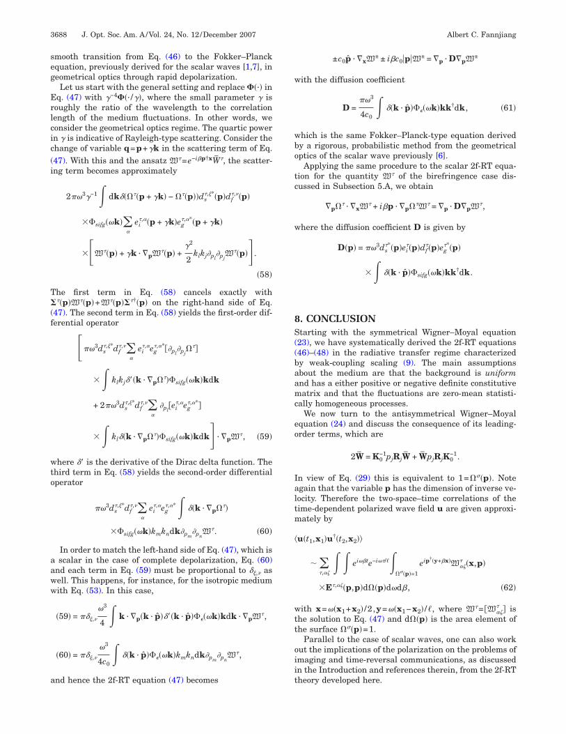
3688 J. Opt. Soc. Am. A/Vol. 24, No. 12 /December 2007 Albert C. Fannjiang
mooth transition from Eq. (46) to the Fokker–Planckquation, previously derived for the scalar waves [1,7], ineometrical optics through rapid depolarization.
Let us start with the general setting and replace ��·� inq. (47) with �−4��· /��, where the small parameter � is
oughly the ratio of the wavelength to the correlationength of the medium fluctuations. In other words, weonsider the geometrical optics regime. The quartic powern � is indicative of Rayleigh-type scattering. Consider thehange of variable q=p+�k in the scattering term of Eq.47). With this and the ansatz W�=e−i�p†xW�, the scatter-ng term becomes approximately
2��3�−1� dk�� ��p + �k� − ��p��ds�,�*�p�df
�,��p�
�sifg��k���
ei�,��p + �k�eg
�,�*�p + �k�
��W��p� + �k · �pW��p� +�2
2klkj�pl
�pjW��p� .
�58�
he first term in Eq. (58) cancels exactly with��p�W��p�+W��p���†�p� on the right-hand side of Eq.
47). The second term in Eq. (58) yields the first-order dif-erential operator
���3ds�,�*df
�,���
ei�,�eg
�,�* �pl�pj
��
�� klkj���k · �p ��sifg��k�kdk
+ 2��3ds�,�*df
�,���
�pl ei
�,�eg�,�*�
�� kl��k · �p ��sifg��k�kdk · �pW�, �59�
here �� is the derivative of the Dirac delta function. Thehird term in Eq. (58) yields the second-order differentialperator
��3ds�,�*df
�,���
ei�,�eg
�,�*� ��k · �p ��
�sifg��k�kmkndk�pm�pn
W�. �60�
In order to match the left-hand side of Eq. (47), which isscalar in the case of complete depolarization, Eq. (60)
nd each term in Eq. (59) must be proportional to ��,� asell. This happens, for instance, for the isotropic mediumith Eq. (53). In this case,
�59� = ���,�
�3
4 � k · �p�k · p����k · p����k�kdk · �pW�,
�60� = ���,�
�3
4c0� ��k · p����k�kmkndk�pm
�pnW�,
nd hence the 2f-RT equation (47) becomes
±c0p · �xW± ± i�c0�p�W± = �p · D�pW±
ith the diffusion coefficient
D =��3
4c0� ��k · p����k�kk†dk, �61�
hich is the same Fokker–Planck-type equation derivedy a rigorous, probabilistic method from the geometricalptics of the scalar wave previously [6].
Applying the same procedure to the scalar 2f-RT equa-ion for the quantity W� of the birefringence case dis-ussed in Subsection 5.A, we obtain
�p � · �xW� + i�p · �p �W� = �p · D�pW�,
here the diffusion coefficient D is given by
D�p� = ��3ds�*�p�ei
��p�df��p�eg
�*�p�
�� ��k · p�sifg��k�kk†dk.
. CONCLUSIONtarting with the symmetrical Wigner–Moyal equation
23), we have systematically derived the 2f-RT equations46)–(48) in the radiative transfer regime characterizedy weak-coupling scaling (9). The main assumptionsbout the medium are that the background is uniformnd has a either positive or negative definite constitutiveatrix and that the fluctuations are zero-mean statisti-
ally homogeneous processes.We now turn to the antisymmetrical Wigner–Moyal
quation (24) and discuss the consequence of its leading-rder terms, which are
2W = K0−1pjRjW + WpjRjK0
−1.
n view of Eq. (29) this is equivalent to 1= ��p�. Notegain that the variable p has the dimension of inverse ve-ocity. Therefore the two-space–time correlations of theime-dependent polarized wave field u are given approxi-ately by
u�t1,x1�u†�t2,x2��
� ��,��
�� ei��te−i��/�� ��p�=1
eip†�y+�x�W��� �x,p�
�E�,���p,p�d �p�d�d�, �62�
ith x=��x1+x2� /2 ,y=��x1−x2� /�, where W�= W��� � is
he solution to Eq. (47) and d �p� is the area element ofhe surface ��p�=1.
Parallel to the case of scalar waves, one can also workut the implications of the polarization on the problems ofmaging and time-reversal communications, as discussedn the Introduction and references therein, from the 2f-RTheory developed here.

AWA
R
I(
It
A1W
C
UwaK
r
2T
h
Albert C. Fannjiang Vol. 24, No. 12 /December 2007 /J. Opt. Soc. Am. A 3689
PPENDIX A: DERIVATION OF THEIGNER–MOYAL EQUATION
pplying the operator Rj� /�xj to W we have
j
�
�xjW�x,p� =
1
�2��3 � e−ip†yRj
�
�xjU1� x
�1+
y
2�1�
�U2†� x
�2−
y
2�2�dy +
1
�2��3 � e−ip†yRj
�U1� x
�1+
y
2�1� �
�xjU2
†� x
�2−
y
2�2�dy,
=1
�2��3 � e−ip†y�1−1Rj
�
�xjU1� x
�1+
y
2�1�
�U2†� x
�2−
y
2�2�dy −
2
�2��3 � e−ip†yRj
�U1� x
�1+
y
2�1� �
�yjU2
†� x
�2−
y
2�2�dy.
ntegrating by parts with the second integral and using6) we obtain
Rj
�
�xjW�x,p� =
2i
�2��3 � e−ip†yK� x
�1+
y
2�2�U1� x
�1+
y
2�1�
�U2†� x
�2−
y
2�2�dy −
2i
�2��3pjRj
�� e−ip†yU1� x
�1+
y
2�1�U2
†� x
�2−
y
2�2�dy.
nserting the spectral representation of K into the equa-ion and using definition (19), we then obtain Eq. (7).
PPENDIX B: CALCULATION OF EQ. (41). Propagation Termse first show that
Tr D�,��†�K0−1Rj�xj
W + �xjWRjK0
−1�� = 2�p � · �xW��� .
onsider the following calculation:
K0−1Rj�xj
W = �p K0−1pjRj� · �xW��
� �e�,�e�,�†
= �p K0−1pjRje�,�� · �xW��
� �e�,�†
− K0−1pjRj �pe�,�� · �xW��
� �e�,�†
= �p � · �xW��� e�,�e�,�† + � � − K0
−1pjRj�
� �pe�,�� · �xW��� �e�,�†.
pon the operation Tr D�,���·�� the second term vanishes,hile the first term reduces to �p � ·�xW��
� by Eq. (28)nd the fact that d�,� is a left eigenvector of the matrix
0−1pjRj with the eigenvalue �.The other term, Tr D�,��†�xj
WRjK0−1�, gives the identical
esult.
. Scattering Kernelhe �s , j� element of the matrix
�F� + K0−1Rj
�
�xjW +
�
�xjWRjK0
−1
= 2i� dq�eiq†x/�1V�q�W1�p −q
2�1�
− W1�p −q
2�2�V†�q�e−iq†x/�2�
as the expression
��,�,�,�
2i�13� dk� ��p + k� − ��p� − i��−1df
�,�*�p + k�fgsi��1k�W��� �p�eg
�,��p�Eij�,���p + k,p� − 2i�1
3
�� dk� ��p +1
2��2
�1+ 1�k� − ��p +
1
2��2
�1− 1�k� − i��−1
�ei�1−�2/�1�k†xW��� �p +
1
2�1 +�2
�1�k�fgsi
* �− �2k�
�eg�,�*�p +
1
2�1 +�2
�1�k�df
�,��p +1
2��2
�1− 1�k�
�Eij�,���p +
1
2�1 +�2
�1�k,p +
1
2��2
�1− 1�k� − 2i�2
3� dk� ��p +1
2�1 −�1
�2�k�

U
at
ATP
R
3690 J. Opt. Soc. Am. A/Vol. 24, No. 12 /December 2007 Albert C. Fannjiang
− ��p −1
2��1
�2+ 1�k� − i��−1
ei�1−�1/�2�k†xW�,�� �p −
1
2��1
�2+ 1�k�fgjn��1k�
�df�,�*�p +
1
2�1 −�1
�2�k�eg
�,��p −1
2��1
�2+ 1�k�Esn
�,���p +1
2�1 −�1
�2�k,p −
1
2��1
�2+ 1�k�
+ 2i�23� dk� ��p� − ��p − k� − i��−1W��
� �p�fgjn* �− �2k�eg
�,�*�p�df�,��p − k�Esn
�,���p,p − k�.
1
1
1
1
1
1
1
1
1
1
22
sing the identity
lim�→0
1
x − i�= i���x� +
1
x
nd the symmetry properties (15), (16), and (27), we ob-ain in the limit �→0 Eq. (46) from Eq. (41).
CKNOWLEDGMENTShis research is supported by Defense Advanced Researchrojects Agency (DARPA) grant N00014-02-1-0603.
EFERENCES1. A. C. Fannjiang, “Two-frequency radiative transfer and
asymptotic solution,” J. Opt. Soc. Am. A 24, 2248–2256(2007).
2. M. Mishchenko, L. Travis, and A. Lacis, MultipleScattering of Light by Particles: Radiative Transfer andCoherent Backscattering (Cambridge U. Press, 2006).
3. L. Mandel and E. Wolf, Optical Coherence and QuantumOptics (Cambridge U. Press, 1995).
4. A. C. Fannjiang, “Information transfer in disordered mediaby broadband time reversal: stability, resolution andcapacity,” Nonlinearity 19, 2425–2439 (2006).
5. A. C. Fannjiang and P. M. Yan, “Multi-frequency imaging ofmultiple targets in Rician fading channels: stability andresolution,” Inverse Probl. 23, 1801–1819 (2007).
6. A. C. Fannjiang, “Space-frequency correlation of classicalwaves in disordered media: high-frequency and small scaleasymptotics,” 80, 14005 (2007).
7. I. V. Lindell, A. H. Sihvola, S. A. Tretyakov, and A. J.Viitanen, Electromagnetic Waves in Chiral and Bi-isotropicMedia (Artech House, 1994).
8. T. H. O’Dell, The Electrodynamics of Magneto-ElectricMedia (North-Holland, 1970).
9. L. D. Landau, E. M. Lifshitz, and L. P. Pitaevskii,Electrodynamics of Continuous Media (ElsevierButterworth-Heinemann, 1984).
0. M. Born and W. Wolf, Principles of Optics, 7th (expanded)ed. (Cambridge U. Press, 1999).
1. W. S. Weiglhofer and A. Lakhtakia, Introduction toComplex Mediums for Optics and Electromagnetics (SPIEPress, 2003).
2. D. K. Cheng and 1. A. Kong, “Covariant descriptions ofbianisotropic media,” Proc. IEEE 56, 248–251 (1968).
3. A. C. Fannjiang, “Mutual coherence of polarized light indisordered media: two-frequency method extended,”submitted to J. Phys. A: Math. Theor. 40, 13667–13683(2007).
4. H. N. Kritikos, N. Engheta, and D. L. Jaggard, “Symmetryin electromagnetic media: a spinor viewpoint,” inElectromagnetic Symmetry, C. E. Baum and H. N. Kritikos,eds. (Taylor & Francis, 1995), pp. 185–230.
5. L. Ryzhik, G. Papanicolaou, and J. B. Keller, “Transportequations for elastic and other waves in random media,”Wave Motion 24, 327–370 (1996).
6. I. Bialynicki-Birula, “Photon wave function,” Prog. Opt. 36,245–294 (1996).
7. V. G. Veselago, “The electrodynamics of substances withsimultaneously negative values of � and �,” Sov. Phys. Usp.10, 509–514 (1968).
8. D. R. Smith, W. Padilla, D. C. Vier, S. C. Nemat-Nasser,and S. Schultz, “A composite medium with simultaneouslynegative permeability and permittivity,” Phys. Rev. Lett.84, 4184–4187 (2000).
9. D. R. Smith, J. B. Pendry, and M. C. K. Wiltshire,“Metamaterials and negative refractive index,” Science305, 788–792 (2004).
0. S. Chandrasekhar, Radiative Transfer (Dover, 1960).1. A. Kokhanovsky, Polarization Optics of Random Media
(Springer, 2003).


![Dielectric Dilemmaclassical equations of electrodynamics, as they are usually written. The equations of Maxwell [1-5] seem perfectly general in a vacuum, but, in the presence of dielectrics](https://img.pdfslide.net/doc/110x75/5f197175d1a5b61e6169ee43/dielectric-dilemma-classical-equations-of-electrodynamics-as-they-are-usually-written.jpg)