TWO-GRID METHODS FOR MAXWELL EIGENVALUE PROBLEMSchenlong/Papers/Maxwell_eig.pdf · The author Liuqiang Zhong was supported by the National Natural ... preconditioned inverse iteration

TWO-GRID METHODS FOR MAXWELL EIGENVALUE PROBLEMS

J. ZHOU∗, X. HU † , L. ZHONG‡ , S. SHU § , AND L. CHEN¶

Abstract. Two new two-grid algorithms are proposed for solving the Maxwell eigenvalue prob-lem. The new methods are based on the two-grid methodology recently proposed by Xu and Zhou(Math. Comp., 70:17–25, 2001), and further developed by Hu and Cheng (Math. Comp. 80:1287–1301, 2011) for elliptic eigenvalue problems. The new two-grid schemes reduce the solution of theMaxwell eigenvalue problem on a fine grid to one linear indefinite Maxwell equation on the same finegrid and an original eigenvalue problem on a much coarser grid. The new schemes, therefore, savetotal computational cost. We also show that the error estimates of the two-grid methods maintainasymptotically optimal accuracy, and the numerical experiments presented confirm the theoreticalresults.

Key words. Two-grid method, Maxwell eigenvalue problem, Edge element

AMS subject classifications. 65N25, 65N30

1. Introduction. In this paper, we develop an efficient algorithm for computingthe Maxwell eigenvalue problem, which is a basic and important computational modelin computational electromagnetism, e.g., in regard to electromagnetic waveguides andresonances in cavities (see, e.g. [7, 12, 33, 39]). The governing equations are

curl(µ−1r curlu) = ω2εru in Ω, (1.1)

div(εru) = 0 in Ω, (1.2)

γtu = 0 on ∂Ω, (1.3)

where Ω ⊂ Rn(n = 2, 3) is a bounded Lipschitz polyhedron domain and γtu is thetangential trace of u. The coefficients µr and εr are the real relative magnetic per-meability and electric permittivity, respectively, that satisfy the Lipschitz continuouscondition, whereas ω is the resonant angular frequency of the electromagnetic wavefor cavity Ω. In the following sections, we will use the conventional notation λ toreplace ω2.

Edge finite element methods for solving the Maxwell eigenvalue problem arewidely used and their convergences have been studied extensively (see [8, 11, 20]and references therein). Imposing the divergence-free constraint in the discretization

∗School of Mathematics in Xiang Tan University, Xiangtan, Hunan, China. [email protected] work of the author Jie Zhou was supported by 2012-2013 China Scholarship Council (CSC) andGraduate Innovation Program of Hunan province in China (CX2012B240).†Department of Mathematics, The Pennsylvania State University, University Park, PA16802.

hu [email protected].‡School of Mathematics Science in South China Normal University, Guangzhou, Guangdong,

China. [email protected]. The author Liuqiang Zhong was supported by the National NaturalScience Foundation of China under the grant 11201159, the Foundation for the Author of NationalExcellent Doctoral Dissertation of PR China under the grant 201212 and the Zhujiang TechnologyNew-Star Foundation of GuangZhou under the grant 2013J2200063.§School of Mathematics in Xiang Tan University, Xiangtan, Hunan, China. [email protected].

The author Shi Shu was supported by Program for Changjiang Scholars and Innovative ResearchTeam in University of China (No. IRT1179), Specialized research Fund for the Doctoral Programof Higher Education (20124301110003) and Scientific Research Fund of Hunan Provincial EducationDepartment (12A138).¶Department of Mathematics, University of California at Irvine, Irvine, CA, 92697.

[email protected]. The author Long Chen was supported by NSF Grant DMS-1115961, andin part by Department of Energy prime award # DE-SC0006903.

1

2 J. Zhou, X. Hu, S. Shu, L. Zhong, and L. Chen

is a challenging task. The divergence-free constraint (1.2) can be dropped from theweak formulation and imposed implicitly. Though dropping the constraint may in-troduce spurious eigenvalues, doing so will not affect the nonzero eigenvalues (see,e.g. [20, 36, 31, 30, 48]). An alternative is the so-called mixed formation. In a mixedformulation, a Lagrange multiplier is introduced to impose the divergence-free con-straint (1.2) in a weak sense. Using the mixed discretization, no spurious eigenvaluewill be introduced. However the resulting linear algebraic system is larger and ofthe saddle point type such that it is difficult to solve (see, e.g.[1, 2, 36]). Anotherapproach is the penalty method which relies on explicitly imposing the divergence-free condition by introducing a penalty term (see, e.g. [9, 17, 31]). Compared withthe discretized linear system that arises from the mixed method, the system from thepenalty method is considerably smaller. However, the penalty method also introducesspurious eigenvalues.

For all the methods referred to Maxwell eigenvalue problems above, a large scalediscrete eigenvalue problem has to be solved, which is very challenging and time-consuming. Multigrid methods for computing eigenvalues of symmetric and positivedefinite cases, e.g., [5, 21, 28, 29, 38] are not applicable directly for the Maxwell eigen-value problems due to the large kernel of the differential operator curl. To steeringthe inverse iterations away from the kernel of curl, Hiptimair and Neymeyr [30] pro-posed the so-called projected preconditioned inverse iteration method (PPINVIT);see also [13] for the extension to the adaptivity. In each inverse iteration, multigridmethods are applied in order to solve a shifted Maxwell equation and an additionalPoisson equation with the purpose of imposing the weak divergence-free constraint.It takes 10-20 iterations to converge to an acceptable tolerance [30].

Here, we focus on speeding up the iterations by using a two-grid approach. Thetwo-grid method, first introduced by Xu [43, 44], has been applied to many problems,such as nonlinear elliptic problems [45], nonlinear parabolic equations [18, 19], Navier-Stokes problems [25, 35], and Maxwell equations [50, 51]. In regard to the presentedstudy, most relevant work is the two-grid method for elliptic eigenvalue problemsdeveloped by Xu and Zhou [46]. The main idea proposed by Xu and Zhou [46] is toreduce the solution of an eigenvalue problem on a given fine grid with mesh size h tothe solution of the same eigenvalue problem on a much coarser grid with mesh sizeH h, which can be easily solved as the size of the discrete eigenvalue problem issignificantly smaller than the original eigenvalue problem on the fine grid, and thesolution of a linear problem on the same fine grid, which can be solved by mature andefficient numerical algorithms.

In this paper, we adopt this idea and develop efficient two-grid methods for solvingthe Maxwell eigenvalue problems. That is we first solve a Maxwell eigenvalue problemon a coarse grid, and then solve a linear Maxwell equation on a fine grid. Essentially,the procedure is similar to performing only one step of the Rayleigh quotient iterationusing a good initial guess from the coarse grid. It provides a competitive approachfor computing the Maxwell eigenvalue problems. Although generalizing the two-gridapproach to the Maxwell eigenvalue problems seems straightforward, several non-trivial theoretical and practical issues must be addressed.

First, it is important to note that the standard two-grid method (Xu and Zhou[46]) for elliptic eigenvalue problems works when the order of error in the L2 normis one order higher than the error in the energy norm. Therefore, on the fine grid,a simple linear equation, which comes from the inverse iteration (or the fixed pointiteration in general), can be used to maintain the asymptotically optimal accuracy for

Two-grid Methods for Maxwell Eigenvalue Problems 3

H2 = h. In terms of approximation of the Maxwell equations, it is well-known thatestablishing an L2 norm error estimate is a very challenging task [52]. For example,for the first family edge element, we cannot expect the error in the L2 norm has higherconvergence rate than the error in the energy norm. As a result, in order to makethe two-grid algorithm work, on the fine grid, we must solve linear Maxwell equationsderived from the shifted inverse iteration. This idea is proposed in [34, 47] as anacceleration scheme for the standard two-grid method of elliptic eigenvalue problems.

For the shifted inverse iteration, we need to solve an indefinite and nearly singu-lar Maxwell equation on the fine grid. However, it is difficult to solve this equationsuch that very efficient solvers are required. Because we are interested in small eigen-values, the wave number of this indefinite Maxwell problem is relatively small. Wewill use the preconditioned minimal residual (P-MINRES) including shift Laplaciantechnique [23, 22] and the HX preconditioner [32] for the corresponding definite lin-ear equation. Again since we are interested in the approximation of eigenvalues, wediscard the standard relative residual norm but use the approximation of eigenvaluesas the stopping tolerance of P-MINRES. Our numerical computation shows that thesolver with the modified stopping tolerance converges in a few steps which is almostuniform with respect to the size of the problem. In summary, we reduce solvingthe Maxwell eigenvalue problem to solving a Maxwell equation for which efficientsolvers/preconditioners are available.

Another problem introduced by the shifted inverse iteration is the divergence-free constraint which only holds weakly on the coarse grid. It is possible to explic-itly impose this constraint on the fine grid by projecting the obtained approximatedeigenfunction on the coarse grid to the discrete divergence-free space on the finegrid by solving an extra Poisson equation. However, our analysis, which is based onthe Helmholtz decomposition and an estimate of the differences between the weaklydivergence-free functions on coarse and fine grids, shows that even without the pro-jection step, our two-grid method produces an approximation λh to λ, and remainsasymptotically convergence rate for H3 = h. When the domain is smooth and convex,the rate of convergence is

|λ− λh| ≤ C(H6 + h2).

Note that H3 = h implies that a very coarse mesh can be used–which saves consider-able computational cost and time, especially in three dimensions. For example, for athree-dimensional unit cube, h = 1/64, the number of unknowns is 1, 872, 064 whereasfor H = h1/3 = 1/4 there are only 604 unknowns.

On the other hand, we require the coarse grid to be fine enough to be able tocapture the information we are interested in. This fact somehow limits us to choosetoo coarse grids in our two-grid algorithms, but it is a standard requirement for solvingeigenvalues.

The rest of this paper is organized as follows. In Section 2, we introduce theMaxwell eigenvalue problem. Section 3 presents new algorithms proposed in this pa-per, as well as some notes about the algorithms. In section 4, we show the errorestimates of our two-grid methods for the Maxwell eigenvalue problem. And, in Sec-tion 5, we give some numerical examples in two and three dimensions to demonstratethe efficiency of our new methods.

2. Preliminary. Denoted by

H0(curl; Ω) =

u ∈ (L2(Ω))2 : curlu ∈ L2(Ω), γtu = 0, (if n = 2)u ∈ (L2(Ω))3 : curlu ∈ (L2(Ω))3, γtu = 0, (if n = 3)


equipped with the norm ‖u‖curl := (‖u‖2 + ‖curlu‖2)12 . The tangential trace is

γtu = u × n in three dimensions, whereas the tangential trace is γtu = u · t in twodimensions, with n denoting the outer unit normal vector and t the tangential vectoron boundary Γ = ∂Ω. Define X := u ∈H0(curl; Ω),div(εru) = 0 in Ω,

The variational form of the Maxwell eigenvalue problem (1.1) - (1.3) is: find(λ,u) ∈ R+ ×X and u 6≡ 0 satisfying

a(u,v) = λ b(u,v), for all v ∈ X, (2.1)

where

a(u,v) = (µ−1r curlu, curlv),

b(u,v) = (εru,v).

We use (·, ·) for the standard L2-inner product and define a weight L2-inner product(·, ·)B = b(·, ·).

It is easy to check that the bilinear form a(u,v) satisfies the following conditions(see Corollary 4.4 in [31]):

a(u,v) ≤ C1‖u‖curl‖v‖curl, for all u,v ∈ X,a(u,u) ≥ C2‖u‖2curl, for all u ∈ X.

Define an operator A : X → X ′ ∼= X such that 〈Au,v〉 = a(u,v); therefore, Ais compact and self-adjoint on X. By virtue of Hilbert-Schmidt theory (see [31,40]), there exists an infinite discrete set of eigenvalues λk and the correspondingeigenfunctions uk ∈ X, k = 1, 2, 3, · · · satisfy (2.1).

As the divergence-free constraint (1.2) is difficult to be imposed in the discretiza-tion, we will consider a modified variational problem: find (λ,u) ∈ R+ ×H0(curl; Ω)and u 6≡ 0 satisfying

a(u,v) = λb(u,v), for all v ∈H0(curl; Ω). (2.2)

That is, we solve the eigenvalue problem in a space larger than X. The eigenfunctioncorresponding to λ 6= 0 remains unchanged [8]. Because for λ 6= 0, by taking v = ∇pin (2.2), p ∈ H1

0 (Ω), we have

a(u,∇p) = λb(u,∇p) = λ(εru,∇p) = 0, for all p ∈ H10 (Ω),

which implies a divergence-free constraint (1.2) in the weak sense. However, now zerois an eigenvalue of (2.2) and the corresponding eigenspace is the infinite dimensionalspace ∇H1

0 (Ω).We will consider the finite element approximation based on the modified vari-

ational form (2.2). Let Th be a conforming triangulation of the domain Ω. Thelowest-order edge element defined on Th is

V h =uh ∈H0(curl; Ω)

∣∣ uh|τ = aτ + bτ × x, for all τ ∈ Th, (2.3)

and the discrete divergence-free space is

Xh =uh ∈ V h

∣∣ b(uh,∇q) = 0, for all q ∈ S0h, (2.4)

where S0h is the standard linear Lagrangian finite element space with zero trace such

that ∇S0h ⊂ V h.


The finite element discretization of (2.2) is: find (λh,uh) ∈ R× V h and uh 6≡ 0satisfying

a(uh,vh) = λhb(uh,vh), for all vh ∈ V h. (2.5)

Based on the same argument, for λh 6= 0, the corresponding finite element approx-imation uh implicitly satisfies the discrete divergence-free constraint, i.e., uh ∈ Xh.Therefore, nonzero eigenvalues λh and the corresponding eigenfuctions uh satisfy

a(uh,vh) = λhb(uh,vh), for all vh ∈ Xh. (2.6)

We use (ui, λi) to denote the continuous eigen-pairs and (uh,i, λh,i) to denote thediscrete eigen-pairs and order them as follows:

λ1 ≤ λ2 ≤ · · · ≤ λi ≤ · · · ,λh,1 ≤ λh,2 ≤ · · · ≤ λh,i ≤ · · · .

The following error estimate, which can be found in [8] (Theorem 5.4), is usefulin our analysis.

Theorem 2.1. Let λi be an eigenvalue of problem (2.1) with multiplicity mi,and denote by M(λi) the corresponding eigenspace. Then, exactly mi eigenvalues ofproblems (2.6) λh,i1 , · · · , λh,imi

converge to λi. By denoting Mh(λi) as the direct sumof the eigenspaces corresponding to λh,i1 , · · · , λh,imi

, we have that there exists h0 suchthat for 0 < h < h0, the following inequalities hold:

|λi − λh,ij | ≤ C(ρ1(h) + ρ2(h))2, for all j = 1, · · · ,mi,σ(M(λi),Mh(λi)) ≤ C(ρ1(h) + ρ2(h)),

(2.7)

where C is a constant independent of h and σ(M(λi),Mh(λi)) denote the gap betweenM(λi) and M(λi), which is defined as

σ(M(λi),Mh(λi)) = max(σ(M(λi),Mh(λi)), σ(Mh(λi),M(λi))),

σ(M(λi),Mh(λi)) = supui∈M(λi)

infui,h∈Mh(λi)

‖ui − ui,h‖curl.

Remark 2.1. Due to the space restriction, we refer to [8] for the definitionsof ρ1, ρ2. Here we only list examples of ρ1, ρ2 related to our work. When Ω isa Lipschitz polyhedron, X ⊂ (H1/2+δ(Ω))3 [26, 6, 40], and consequently ρ1(h) =

ρ2(h) = O(h1/2+δ) for some 0 < δ ≤ 1

2. And, when Ω is smooth or convex, δ = 1/2

and ρ1(h) = ρ2(h) = O(h). The details can be found in [8]. 2

At the end of this section, we give an important identity that relates the error inthe eigenvalue to the eigenfunction approximation. The proof is standard and can befound, for example, in Lemma 3.1 of [4].

Proposition 2.2. Let (λ,u) be an eigen-pair of (2.1) or (2.2) with λ 6= 0. Forany w ∈H0(curl; Ω)\0, we have

a(w,w)

b(w,w)− λ =

a(w − u,w − u)

b(w,w)− λb(w − u,w − u)

b(w,w).

3. Two-grid Methods. In this section, we present our two-grid methods for theMaxwell eigenvalue problems. We will prove the error estimates in the next section.


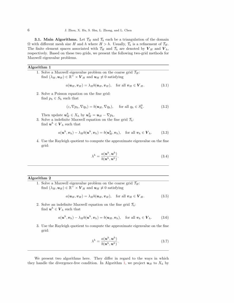
3.1. Main Algorithms. Let TH and Th each be a triangulation of the domainΩ with different mesh size H and h where H > h. Usually, Th is a refinement of TH .The finite element spaces associated with TH and Th are denoted by V H and V h,respectively. Based on these two grids, we present the following two-grid methods forMaxwell eigenvalue problems.

Algorithm 1

1. Solve a Maxwell eigenvalue problem on the coarse grid TH :find (λH ,uH) ∈ R+ × V H and uH 6≡ 0 satisfying

a(uH ,vH) = λHb(uH ,vH), for all vH ∈ V H . (3.1)

2. Solve a Poisson equation on the fine grid:find ph ∈ Sh such that

(εr∇ph,∇qh) = b(uH ,∇qh), for all qh ∈ S0h. (3.2)

Then update uhH ∈ Xh by uhH = uH −∇ph.3. Solve a indefinite Maxwell equation on the fine grid Th:

find uh ∈ V h such that

a(uh,vh)− λHb(uh,vh) = b(uhH ,vh), for all vh ∈ V h. (3.3)

4. Use the Rayleigh quotient to compute the approximate eigenvalue on the finegrid:

λh =a(uh,uh)

b(uh,uh). (3.4)

Algorithm 2

1. Solve a Maxwell eigenvalue problem on the coarse grid TH :find (λH ,uH) ∈ R+ × V H and uH 6≡ 0 satisfying

a(uH ,vH) = λHb(uH ,vH), for all vH ∈ V H . (3.5)

2. Solve an indefinite Maxwell equation on the fine grid Th:find uh ∈ V h such that

a(uh,vh)− λHb(uh,vh) = b(uH ,vh), for all vh ∈ V h. (3.6)

3. Use the Rayleigh quotient to compute the approximate eigenvalue on the finegrid:

λh =a(uh,uh)

b(uh,uh). (3.7)

We present two algorithms here. They differ in regard to the ways in whichthey handle the divergence-free condition. In Algorithm 1, we project uH to Xh by


solving one Poisson equation. However, in Algorithm 2, we skip this step. Our errorestimates in the next section prove that both algorithms are effective. Algorithm 2 ischeaper in terms of computational cost and, consequently, more efficient. Therefore,we recommend to use it in preference to Algorithm 1. On the coarse grid, we solvea Maxwell eigenvalue problem based on the variational form (2.5). As the coarsegrid problem is small, any robust method can be used in this step. We assume thatsolving the Maxwell eigenvalue problem on the coarse grid is inexpensive and thatthe total computational work is negligible compared with the work associated to thelinear system on the fine grid.

Remark 3.1. Algorithm 1 and 2 can be naturally used to compute multipleeigenvalues as long as the coarse grid is fine enough. Assume that an eigenvalue λ hasmultiplicity q and its corresponding eigenfunctions are u1,u2, · · · ,uq. In our two-gridalgorithms, we first need to compute q approximated eigenfunctions u1

H ,u2H , · · · ,u

qH

on the coarse grid. Then we use each umH , m = 1, 2, . . . , q, to proceed the two-gridalgorithms. For example, in Algorithm 2, we use umH , m = 1, 2, . . . , q in (3.6) tocompute uh,m, m = 1, 2, . . . , q. Finally, we compute the Rayleigh quotient of uh,m,m = 1, 2, . . . , q to get q approximate eigenvalues λh,m, m = 1, 2, . . . , q on the fine level.These eigenvalues are approximations of the eigenvalue λ with multiplicity q and thespace spanned by uh,m, m = 1, 2, . . . , q is an approximation of the eigenspace spannedby um, m = 1, 2, . . . , q, of the eigenvalue λ. Note that the computed eigenfunctionsuh,m, m = 1, 2, . . . , q may not be orthogonal but an orthogonal basis of the spacespanned by uh,m, m = 1, 2, . . . , q can be easily obtained by an orthogonalizationprocedure, for example, Gram-Schmidt algorithm. 2

Remark 3.2. Similar to the multiple eigenvalues case discussed in Remark 3.1,Algorithm 1 and 2 can be naturally used to compute clustered eigenvalues as longas the coarse grid is fine enough. For the sake of simplicity, assume two eigenvaluesλ1 and λ2 are close but not equal to each other. We require the coarse level is fineenough to capture the gap between two different eigenvalues, i.e., we should be ableto get two approximations λH,1 and λH,2, which approximate λ1 and λ2, respectively.Then we can proceed the two-grid algorithms as discussed in Remark 3.1 and get twoapproximate eigen-pairs (λh1 ,u

h1 ) and (λh2 ,u

h2 ) on the fine level. The error estimate

we presented later will be amplified by the factor 1/|λ1 − λ2|. 2

On the fine grid, it is necessary to solve an indefinite Maxwell equation, which isbased on the idea of using the approximation on the coarse grid as an initial guess inthe Newton’s iteration. As we shall explain next, this is different from the classicaltwo-grid method for eigenvalue problems.

Consider the abstract eigenvalue problem Au = λu with a compact operator A.If we use the approximation on the coarse grid uH and λH as an initial guess, andapply one step of fixed-point iteration, we obtain Auh = λHuH . Roughly speaking,this describes the two-grid method proposed by Xu and Zhou [46]. Due to the linearconvergence rate of the fixed-point iteration, if

‖u− uH‖+ |λ− λH | = O(H2), (3.8)

then we can expect the resulting two-grid method has asymptotical convergence rateO(h)+O(H2). However, for the first family edge element, an optimal L2 error estimatesuch as (3.8) is not available as the polynomial space is incomplete. Consequently,two-grid methods based on the fixed-point iteration may not work.

The two-grid algorithms we propose are based on the generalization of the accel-erated two-grid scheme proposed by Hu and Cheng [34], which can also be viewed as


a variant of the Newton’s method for the eigenvalue problems. Let us reformulate theeigenvalue problem as the following nonlinear problem:

F (uh, λh) := Ahuh − λhuh = 0.

By applying Newton’s method with uH and λH from the coarse grid as the initialguess, we have

∇F (uH , λH)

(δuδλ

)= −F (uH , λH)

and more specifically

(Ah − λHI − uH

)(δuδλ

)= −(AhuH − λHuH),

which can be reformulated as

(Ah − λHI)(uH + δu) = δλ uH . (3.9)

We cannot solve one equation (3.9) since it involves two unknowns δu and δλ. How-ever, a crucial observation is that δλ on the right-hand side can be treated as a scalingwhich will not affect the Rayleigh quotient of the eigenfunction. More precisely, con-sider the problem without the scaling δλ on the right-hand side:

(Ah − λHI)uh = uH . (3.10)

It is, therefore, easy to show that δλ uh = uh := uH + δu. Moreover, an importantfact is that

λh =(Ahuh, uh)

(uh, uh)=

(Ahuh, uh)

(uh, uh).

This means that solving the problem (3.10) could lead to the same approximationof the eigenvalue as can be achieved with the Newton’s iteration, which suggests thesecond step in our two-grid algorithms.

3.2. Efficiency and Solver. Our main reason for proposing the two-grid meth-ods is to address the high computational cost of solving a large-size eigenvalue prob-lem. Among the existing methods for Maxwell eigenvalue problem, the standardinverse iteration is one of the most popular methods, although, it is difficult to find agood initial vector and it is necessary to solve a large positive semidefinite Maxwellequation. Furthermore, the solution must be projected onto the orthogonal comple-ments of the kernels in every iteration.

A two-grid scheme can reduce the discrete eigenvalue problem on a fine grid Thto the same problem on a much coarser grid TH and only one shifted inverse iterationon the fine grid Th. The accuracy of O(h2 +H6) (assume the domain is smooth andconvex) as shown in the next section allows us to use a very coarse grid, which makesthe computational cost on the coarse grid negligible. Therefore, the dominate cost ofthe two-grid methods is solving an indefinite and nearly singular Maxwell problem onthe fine grid.

For the coarse grid eigenvalue problem (3.5), it is a generalized algebraic eigen-value problem which is small in size. We can solve the problem directly, for example,


using the eigs function in MATLAB. For (3.6) on the fine grid, we need to solve anindefinite Maxwell equation. As we are usually interested in several small eigenvalues,we combine the shift Laplacian technique [15, 22] with the HX-preconditioner [32] inorder to design an efficient solver.

Write (3.6) in the following matrix form:

(Ah − λHMh)uh = b. (3.11)

In these notations, Ah = (a(φj ,φi))ij is the stiffness matrix, Mh = (b(φj ,φi))ij isthe mass matrix, and b is the load vector. This is a symmetric indefinite system.We choose the MINRES method with the shifted Laplacian preconditioner (Ah +λHMh)−1, which is further approximated by the well-known HX preconditioner [32].In our numerical experiments, one step of the HX preconditioner is used in everyMINRES iteration and the numerical results show that such a solver is effective androbust.

For the stopping criterion of the MINRES method, we choose the accuracy ofε = |λih − λi+1

h |/λi+1h , where i means the iteration step, rather than the standard

relative residual ‖b − (Ah − λHMh)uh,i‖/‖b‖. We made this choice for the follow-ing two reasons: (1) the final goal is to solve an eigenvalue problem and approxi-mate the eigenvalues; and (2) the iteration error is almost entirely with in the spacespanned by the eigenvectors (see, e.g. [34]), such that the error will not affect theRayleigh quotient. An alternative stopping criterion is ε = ‖ri+1 − ri‖/‖ri‖ whereri = Ahu

h,i − λihMhuh,i. Note that in the definition of ri, λih instead of λH is used

since the eigen-pair we are computing is (λih, uh,i). We can also use the stopping

criterion ε = min|λih − λi+1h |/λ

i+1h , ‖ri+1 − ri‖/‖ri‖ which includes both eigenvalues

and eigenfunctions. These choice of accuracy reduces the number of iteration stepsdramatically comparing with the standard choice of the relative residual.

Remark 3.3. When λH is close to the eigenvalue λh on the fine level, theindefinite problems on the fine level in our two-grid algorithms become nearly singularand seem to be more challenging to solve. This problem has been much discussed inthe literature in the context of general inverse power method. As shown in, e.g.,[27, 42, 41], the near-singularity of this system hardly presents a problem due to thefact that, for eigenvalue problem, the near null space of this system is exactly spannedby the eigenfunctions that we are interested in. A detailed discussion can be found,for example, in Remark 3.2, [34]. 2

4. Error Estimate. In this section, we will give error estimate of both ourtwo-grid methods, Algorithm 1 and 2, for the Maxwell eigenvalue problems.

4.1. Error Estimate of Algorithm 1. Assuming that the eigenvalue λ hasmultiplicity q, let

M(λ) = u ∈ X : u is an eigenvector of (2.1) corresponding to λ

be the eigenspace corresponding to the eigenvalue λ. Let Λ = λh,i, i = 1, . . . , q beapproximated eigenvalues of eigenvalue λ by solving the variational problem (2.5).Let uh,i denote the eigenvectors corresponding to λh,i, for i = 1, · · · , q. Similarly, let

Mh(λ) = spanuh,1,uh,2, · · · ,uh,q

be the approximate eigenspace corresponding to the eigenvalue λ.


Given a positive constant µ, define the following bilinear form:

a+µ (u,v) = a(u,v) + µb(u,v), for all u, v ∈ X. (4.1)

It is well-known that (see Lemma 4.10, [40])

|a+µ (u,v)| ≤ C‖u‖curl‖v‖curl, for all u,v ∈ X,|a+µ (u,u)| ≥ C‖u‖2curl, for all u ∈ X,

where the constant C depends on µr, εr, and µ but is independent of u and v. Asimilar statement is also true for space Xh, i.e.,

|a+µ (uh,vh)| ≤ C‖uh‖curl‖vh‖curl, for all uh,vh ∈ Xh,

|a+µ (uh,uh)| ≥ C‖uh‖2curl, for all uh ∈ Xh,

where the constant C also depends on µr, εr, and µ but is independent of uh, vh, andthe mesh size h. Moreover, we can define the operators K : (L2(Ω))n → (L2(Ω))n

and Kh : (L2(Ω))n → (L2(Ω))n such that

a+µ (Kf,v) = −2µb(f,v), for all v ∈ X, (4.2)

a+µ (Khf,vh) = −2µb(f,vh), for all vh ∈ Xh. (4.3)

The following lemma has been shown in [40].Lemma 4.1 (Theorem 4.11, [40]). The operators K and Kh are bounded and

compact from L2(Ω) into L2(Ω). In addition,

‖Kf‖curl ≤ C‖f‖L2 , (4.4)

‖Khf‖curl ≤ C‖f‖L2 , (4.5)

where the constants C only depend on µr, εr, and µ.Both K and Kh are compact and their eigenvalues are −2µ/(λ+µ) and −2µ/(λh+

µ), respectively, where λ and λh are eigenvalues of the Maxwell eigenvalue problem(2.1) and (2.6). Therefore, we have the following estimate for the operator (I+Kh)−1

restricted to the orthogonal complement of Mh(λ) in Xh, which will play an importantrole in the error analysis for our two-grid methods.

Lemma 4.2. Let M⊥h (λ) denote the orthogonal complement of Mh(λ) in Xh withrespect to b(·, ·). Then we have

‖(I +Kh)−1‖M⊥h (λ)→M⊥

h (λ) =

(minλh,j 6∈Λ

∣∣∣∣λh,j − µλh,j + µ

∣∣∣∣)−1

. (4.6)

Let ρ = minλj 6=λ

|λj − λ|. Assume that h is small enough such that |λh,j − λj | ≤1

4ρ, for

λj 6= λ and assume that |µ− λ| ≤ 1

4ρ. Then we have

minλh,j 6∈Λ


∣∣∣∣ ≥ ρ

4λ+ 2ρ=: C−1

ρ,λ > 0.

Proof. The identity (4.6) directly follows from the fact that

(I +Kh)−1 : M⊥h (λ)→M⊥h (λ),


and the operator (I +Kh)−1 is self-adjoint with respect to the inner product b(·, ·).Note that |λh,j − µ| ≥ ||λj − λ| − |µ− λ| − |λj − λh,j || ≥

1

2ρ, then we have 0 <

λh,j ≤ µ−1

2ρ or λh,j ≥ µ+

1

2ρ. Therefore,

minλh,j 6∈Λ


∣∣∣∣ ≥ min0<x≤µ− 1

2ρ or x≥µ+ 12ρ

∣∣∣∣x− µx+ µ

∣∣∣∣ =ρ

4µ+ ρ≥ ρ

4λ+ 2ρ> 0. (4.7)

The following lemma shows that the discrete divergence-free function can be ap-proximated by a continuous divergence-free function. Such a construction for the caseεr = 1 is used, for example, in Girault [24] and [3], and a detailed proof can be foundin [31, 40].

Lemma 4.3 (Lemma 4.5, [31]). Let uh ∈ Xh and Ω be a bounded Lipschitzpolyhedron. There exists a u ∈H0(curl; Ω) satisfying

curlu = curluh, div(εru) = 0, in Ω, (4.8)

and

‖u− uh‖0 ≤ Ch1/2+δ‖curluh‖0 (4.9)

where the constants C and 0 < δ ≤ 1/2 are independent of h, u, and uh.The following lemma, which can be found in [3], provides an error estimate for

the solution of the Poisson problem (3.2) on the fine grid in the two-grid algorithm.Lemma 4.4 (Proposition 4.4, [3]). Under the assumptions of Lemma 4.3, let

ph,uhH ,uH be defined as in Algorithm 1. Then we have

‖∇ph‖L2 = ‖uH − uhH‖L2 ≤ CH1/2+δ‖curluH‖L2 , (4.10)

where the constant C and 0 < δ ≤ 1/2 are independent of h and uH .Proof. Note that uhH = uH −∇ph,

b(uhH ,∇qh) = b(uH −∇ph,∇qh) = 0, for all qh ∈ S0h,

which implies that uhH is discrete divergence-free in S0h. Then, by Lemma 4.3, there

exists a w ∈H0(curl; Ω) satisfying

curlw = curluhH , div(εrw) = 0, (4.11)

‖w − uhH‖0 ≤ Ch1/2+δ‖curluhH‖0. (4.12)

Furthermore, (3.1) implies that uH is discrete divergence-free in S0H . Based on

Lemma 4.3 again, there exists a w ∈H0(curl; Ω) that satisfies

curl w = curluH , div(εrw) = 0 (4.13)

‖w − uH‖0 ≤ CH1/2+δ‖curluH‖0. (4.14)

In view of (4.11) and (4.13), we know that

w − w ∈ X, and curl(w − w) = curl(uhH − uH) = curl(−∇ph) = 0,

which implies w = w.


Finally, as uhH = uH −∇ph and w = w, by the inequalities (4.12) and (4.14),

‖∇ph‖L2 = ‖uH − uhH‖L2 ≤ ‖uH − w‖L2 + ‖w − uhH‖L2 ≤ CH1/2+δ‖curluH‖0.

This completes the proof.Now we are ready to provide an error estimate of Algorithm 1.Theorem 4.5. Let λH and (λh,uh) be computed by Algorithm 1 and λH is an

approximation of the eigenvalue λ. Under the assumptions of Lemma 4.2 and 4.4,there exists an eigenfunction u ∈M(λ), such that

minα∈R‖u− αuh‖L2 ≤ C(h1/2+δ +H3(1/2+δ)), (4.15)

minα∈R‖u− αuh‖curl ≤ C(h1/2+δ +H3(1/2+δ)). (4.16)

And for the eigenvalue, we have

|λ− λh| ≤ C(h1+2δ +H3(1+2δ)), (4.17)

where the constants C depend only on µr, εr, ρ, λ, and u, and δ ∈ (0, 1/2] dependsonly on the domain.

Proof. Let us define the operator Ah : Xh → Xh as

(Ahu,v)B = a(u,v) for all u,v ∈ Xh.

Suppose eigenvalue λ is a multiple eigenvalue with multiplicity q. Let the eigen-pair(λh,i,uh,i), for some i ∈ 1, . . . , q, be one approximation of (λ,u) by solving (2.5)which satisfies the relation (2.6)

Ahuh,i = λh,iuh,i in Xh. (4.18)

If λH = λh,j for some j ∈ 1, . . . , q. Then the estimate is obtained by Theorem2.1. We thus assume λH 6= λh,j for all j ∈ 1, . . . , q. Since λH approximates λ,we also assume the coarse grid size H is fine enough such that λH is not equal toeigenvalues of Ah other than λh,j . Therefore Ah − λHI is invertible. Let uh ∈ Xh bethe solution of the operator equation:

(Ah − λHI)uh = (λh,i − λH)uhH in (Xh, (·, ·)B). (4.19)

Here (Xh, (·, ·)B) means the Hilbert space Xh endowed with inter product (·, ·)B .From (4.18) and (4.19), we have the error equation

(Ah − λHI)(uh,i − uh) = (λh,i − λH)(uh,i − uhH), in (Xh, (·, ·)B). (4.20)

We decompose uh,i − uhH on the right hand side as

uh,i − uhH = (uh,i − EhuhH) + (EhuhH − uhH),

where Eh is the orthogonal projection of Xh, w.r.t to (·, ·)B , onto Mh(λ). We canthus rewrite the error equation (4.20) as

(Ah − λHI)(uh,i − uh) = (λh,i − λH)(EhuhH − uhH), (4.21)

where uh,i = uh,i − (λh,i − λH)(Ah − λHI)−1(uh,i − EhuhH).


Now it is crucial to observe that Ah − λHI : Mh(λ) → Mh(λ) and Ah − λHI :M⊥h (λ)→M⊥h (λ) are isomorphism since Mh(λ) is an eigenspace of operator Ah andλH is not an eigenvalue of Ah.

Then since uh,i − EhuhH ∈Mh(λ) and uh,i ∈Mh(λ), we conclude uh,i ∈Mh(λ).

Similarly (EhuhH − uhH) ∈M⊥h (λ) implies (uh,i − uh) ∈M⊥h (λ).

Following a similar argument to that in [40], we can define a vector Fh,i ∈ Xh

such that

(Ah + λHI)Fh,i = (λh,i − λH)(EhuhH − uhH) in Xh

Therefore, we have Fh,i ∈M⊥h (λi) and

‖Fh,i‖curl ≤ C|λh,i − λH |‖EhuhH − uhH‖L2 .

By the definition of Kh with µ = λH , the problem (4.21) is equivalent to

(I +Kh)(uh,i − uh) = Fh,i.

Therefore, we have

‖uh,i − uh‖L2 ≤ ‖(I +Kh)−1‖M⊥h (λ)→M⊥

h (λ)‖Fh‖L2

≤ Cρ‖Fh,i‖L2

≤ CρC|λh,i − λH |‖EhuhH − uhH‖L2 .

According to the standard error estimate of uH (see [8, 31]), there exists uh ∈Mh(λ)such that ‖uh − uH‖L2 ≤ CH1/2+δ. Therefore, we have

‖EhuhH − uhH‖L2 ≤ ‖uh − uhH‖L2 ≤ ‖uh − uH‖L2 + ‖uH − uhH‖L2 ≤ CH1/2+δ

where we use Lemma 4.4 in the last inequality. Then due to the standard estimate|λh,i − λH | ≤ |λ− λh,i|+ |λ− λH | ≤ CH1+2δ, we have

‖uh,i − uh‖L2 ≤ CH3/2+3δ. (4.22)

In view of the above procedure, we also have

‖Fh,i‖curl ≤ C|λh,i − λH |‖EhuhH − uhH‖L2 ≤ CH3/2+3δ. (4.23)

On the other hand, (uh,i − uh) = Fh,i −Kh,i(uh,i − uh) such that

‖curl(uh,i − uh)‖L2 ≤ ‖uh,i − uh‖curl ≤ C(‖Fh,i‖curl + ‖uh,i − uh‖L2) ≤ CH3/2+3δ,

where (4.23), Lemma 4.1 and the inequality (4.22) are used.Moreover, since σ(M(λ),Mh(λ)) ≤ Ch1/2+δ, there exists u ∈ M(λ) such that

‖u− uh,i‖curl ≤ Ch1/2+δ and consequently

‖u− uh‖L2 ≤ ‖u− uh,i‖L2 + ‖uh,i − uh‖L2 ≤ C(h1/2+δ +H3/2+3δ), (4.24)

‖u− uh‖curl ≤ ‖u− uh,i‖curl + ‖uh,i − uh‖curl ≤ C(h1/2+δ +H3/2+3δ). (4.25)

Note that uh = (λh,i − λH)uh. Then the estimates (4.15) and (4.16) follow directly.


Using the triangle inequality and ‖u‖L2 = 1, we have

‖uh‖L2 ≥ ‖u‖L2 − ‖u− uh‖L2 ≥ 1− CH3/2+3δ. (4.26)

Hence, we obtain a lower bound of ‖uh‖L2 under the assumption H is small enough.To get the estimate of the eigenvalue, by Proposition 2.2, the boundedness of µr

and εr, (4.26) and the boundedness of λ , we have

|λh − λ| =

∣∣∣∣∣a(uh − u, uh − u)

b(uh, uh)− λb(u

h − u, uh − u)

b(uh, uh)

∣∣∣∣∣≤ C

(‖curl(u− uh)‖2L2 + λ‖u− uh‖2L2

)≤ C(h1+2δ +H3+6δ),

which gives the error estimate for the eigenvalue (4.17).Remark 4.1. For the case in which domain Ω is smooth or convex, we have

δ = 1/2 and

minα∈R‖u− αuh‖L2 + min

α∈R‖u− αuh‖curl ≤ C(h+H3),

|λ− λh| ≤ C(h2 +H6).

4.2. Error Estimate of Algorithm 2. Working in the divergence-free spaceXh requires solving an extra Poisson problem on the fine grid. In this section, wediscuss the convergence of Algorithm 2 based on the standard edge element spacesV H and V h and our analysis proves that this extra step can be skipped. Note that,V H ⊂ V h.

In order to analyze Algorithm 2, again, we introduce the following auxiliary prob-lem on the fine grid:

a(uh,vh)− λHb(uh,vh) = (λh,i − λH)b(uH ,vh), for all vh ∈ V h.

And recall that the eigen-pair (λh,i,uh,i) ∈ R+ ×Xh satisfies

a(uh,i,vh) = λh,ib(uh,i,vh), for all vh ∈ V h,

and thus obtain the following equation which is similar to (4.20) but imposed on V h

instead of Xh:

a(uh,i−uh,vh)−λHb(uh,i−uh,vh) = (λh,i−λH)b(uh,i−uH ,vh), vh ∈ V h. (4.27)

Note that uh,i − uh = eh,i +∇ph for some eh,i ∈ Xh and ph ∈ S0h, where ph can

be determined by solving

− λH(εr∇ph,∇qh) = (λh,i − λH)b(uh,i − uH ,∇qh), for all qh ∈ S0h. (4.28)

Following [40], we can easily estimate ph as following.Lemma 4.6. Under the assumptions of Lemma 4.4, we have

‖∇ph‖L2 =|λh,i − λH |

λH‖∇ph‖L2 ≤ CH3/2+3δ, (4.29)


where ph is defined by (3.2) and the constant C and δ ∈ (0, 1/2] are independent ofH.

Proof. Using (4.28), uh,i ∈ Xh and (3.2), we have

λH(εr∇ph,∇qh) = (λh,i−λH)b(uH ,∇qh) = (λh,i−λH)(εr∇ph,∇qh), for all qh ∈ S0h.

Then the result follows from Lemma 4.4 directly.Theorem 4.7. Let λH and (λh,uh) be computed by Algorithm 2 and λH is an

approximation of the eigenvalue λ. Under the assumptions of Lemma 4.2 and 4.4,then there exists an eigenfunction u ∈M(λ) such that

minα∈R‖u− αuh‖L2 ≤ C(h1/2+δ +H3(1/2+δ)), (4.30)

minα∈R‖u− αuh‖curl ≤ C(h1/2+δ +H3(1/2+δ)). (4.31)

And for the eigenvalue, we have

|λ− λh| ≤ C(h1+2δ +H3(1+2δ)), (4.32)

where the constant C and 0 < δ ≤ 1/2 depend only on µr, εr, ρ, λi, and u.Proof. Substituting uh,i−uh = eh,i+∇ph into (4.27), and using uhH = uH−∇ph,

then for any vh ∈ Xh, we have

a(eh,i,vh)−λHb(eh,i,vh) = (λh,i−λH)b(uh,i−uH ,vh) = (λh,i−λH)b(uh,i−uhH ,vh),

where we use b(∇ph,vh) = 0 in the first identity and b(∇ph,vh) = 0 in the secondidentity, for all vh ∈ Xh. Now, we can rewrite the above identity in the operatorequation:

(Ah − λHI)eh,i = (λh,i − λH)(uh,i − uhH) in Xh (4.33)

Comparing (4.33) with (4.20), we have eh,i = uh,i − uh, where uh is defined in

(4.19). Hence, we have uh = uh −∇ph.Therefore, based on (4.24) and (4.25), there exists a u ∈M(λ) such that

‖u− uh‖L2 ≤ ‖u− uh‖L2 + ‖∇ph‖L2 ≤ C(h1/2+δ +H3(1/2+δ)). (4.34)

and similarly

‖u− uh‖curl ≤ ‖u− uh‖curl + ‖∇ph‖L2 ≤ C(h1/2+δ +H3(1/2+δ)). (4.35)

This leads to (4.30) and (4.31). For the eigenvalue, using the triangle inequality and‖u‖L2 = 1, we have

‖uh‖L2 ≥ ‖u‖L2 − ‖u− uh‖L2 ≥ 1− CH3/2+3δ. (4.36)

(4.32) follows from Proposition 2.2.Remark 4.2. When Ω is smooth or convex, we have δ = 1/2 and

minα∈R‖u− αuh‖L2 + min

α∈R‖u− αuh‖curl ≤ C(h+H3),

|λ− λh| ≤ C(h2 +H6).


5. Numerical Experiments. In this section, we will report several numericalexperiments in two and three dimensions to verify the effectiveness and robustnessof Algorithm 2. We implemented these experiments using the iFEM package [16].We did the computation in double decision, but only display 6 digits after decimal intables, which are accurate enough for quantity bigger than 10−6.

Example 5.1. Consider the Maxwell eigenvalue problem (1.1) - (1.3) on thetwo-dimensional domain Ω = (0, 1)× (0, 1) and µr = εr = 1 in Ω. It is easy to showthat λ1 = λ2 = π2 and λ3 = 2π2.

The results shown in Table 5.1-5.3 verify the theoretical expectations. Let λk,Hand λk,h denote the eigenvalues computed by solving the eigenvalue problem (3.5)on the coarse grid TH and the refined grid Th respectively, and let λhk denote theeigenvalue obtained by Algorithm 2, here k = 1, 2, 3. The coarse mesh TH is theuniform triangular mesh. The fine grid Th is obtained by applying several uniformrefinements (every triangle is divided into four congruent triangles) from TH .

We design several tests to verify our error estimate. First, we fix a coarse meshand vary fine mesh. The mesh sizes satisfy the relation h2 ≥ H6, thus O(H6) issmaller than O(h2). From Table 5.1, it is evident that the approximation rate isindeed O(h2). Second, we fix a fine mesh and vary the coarse mesh subject to theconstraint h2 ≥ H6. Table 5.2 shows that we can obtain the same level of accuracyby using different coarse meshes. In Table 5.2, “ − ” means that the computer weuse does not have enough memory to solve the eigenvalue problem with direct solverswhen the mesh size is too small. Third, in Table 5.3, we vary both the coarse and finemeshes at the same time, subjected to h2 = H6, i.e., O(h2 +H6) = O(H6). Similarly,we only need pay attention to whether the numerical results satisfy |λ−λh| = O(H6).In fact, it is easy to find that the convergence rate is O(H6), as shown in Table 5.3.

To sum up, we used three different approaches to show that the numerical resultsare consistent with our theory. Tables 5.1- 5.3 verify that |λ − λh| = O(h2 + H6).Further, the solver introduced before is efficient. The most time-consuming part ofthe solver is the HX preconditioner. Therefore, we report the number of calls of theHX preconditioner. We compare our method with the inverse iteration method forcomputing eigenvalues. For the first eigenvalue, at each inverse iteration step, PCGusing HX preconditioner typically needs 5− 6 iterations and typically 10 steps of in-verse iteration are needed. For other eigenvalues, a shifted indefinite and near singularMaxwell equation should also be solved and again around 10 steps of inverse iterationare needed to converge. Our method behaves essentially like one inverse iterationand thus reduces the total computational cost. We choose HX preconditioner as thecomputational cost unit because other measurements, such as CPU time, depends onthe programming language, computational environment, and many other facts.

Example 5.2. Consider the Maxwell eigenvalue problem on a 2D L-shaped do-main Ω = (−1, 1)2/(0, 1)× (−1, 0) and µr = εr = 1. λ1 = 1.47562182 (see [10]).

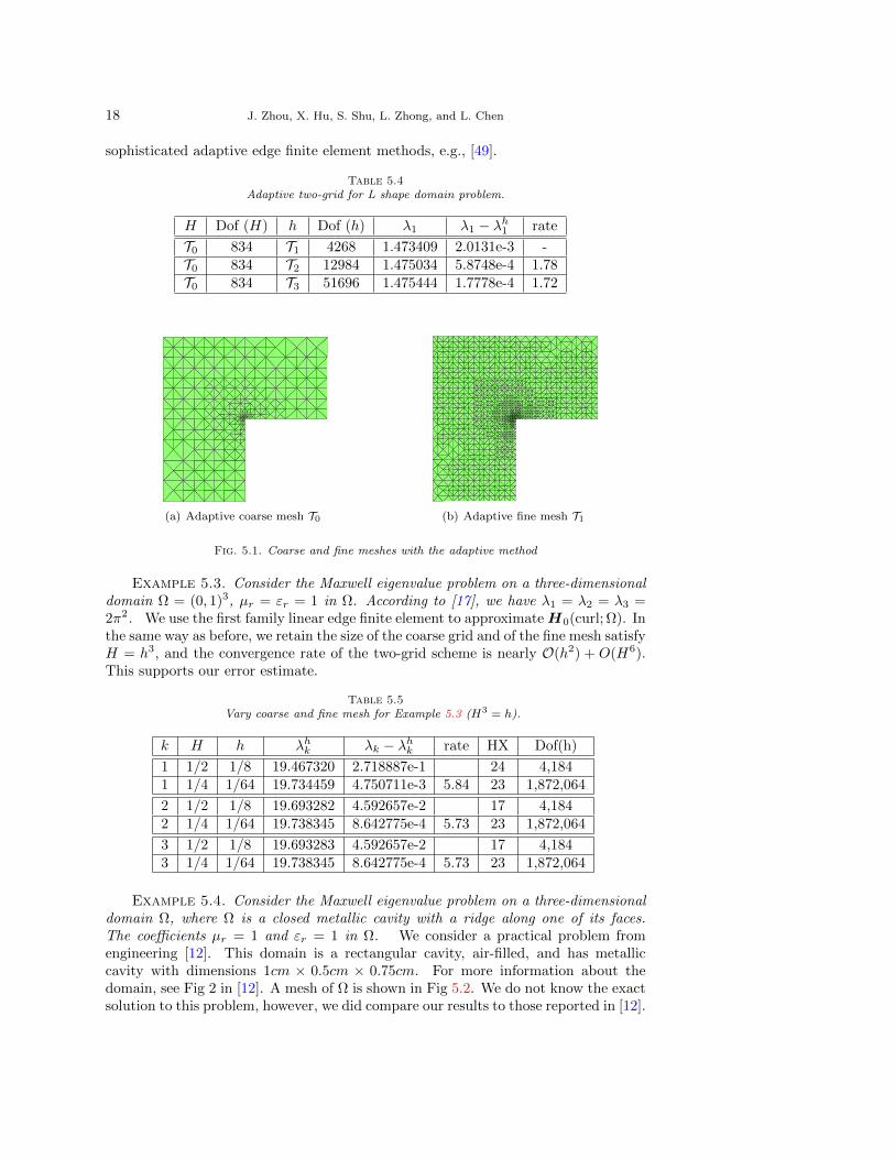
We consider an L-shaped domain problem. The solution has a singularity at theorigin and δ 6= 1/2 in the analysis. We use a simple adaptive method for the two-grid method. The coarse grid T0 used in this numerical experiment is an adaptivelyrefined grid. Ti is obtained by uniform refinement (every triangle is divided into four)of Ti−1 for i = 1, 2, 3; see Fig 5. From Table 5.4, we know that this simple adaptivetwo-grid method is also efficient for the L-shaped domain. Due to the singularity ofthe solution and the refinement strategy we use, the rate is not close to the secondorder. Here for adaptive grids, the second order h2 is replaced by N−1 where N isthe number of unknowns. We would expect optimal rate of convergence with more


Table 5.1Fixed coarse mesh and varied fine meshes for Example 5.1.

k H h λk,H λk,h λhk λk − λhk rate HX

1 1/16 1/32 9.867576 9.864823 9.869102 5.018558e-4 221 1/16 1/64 9.867576 9.868408 9.869479 1.251880e-4 2.00 281 1/16 1/128 9.867576 9.869305 9.869577 3.125953e-5 2.00 311 1/16 1/256 9.867576 9.869596 9.869597 7.458585e-6 2.04 30

2 1/16 1/32 9.867577 9.869102 9.869102 5.018558e-4 222 1/16 1/64 9.867577 9.869479 9.869479 1.251880e-4 2.00 282 1/16 1/128 9.867577 9.869573 9.869573 3.125953e-5 2.00 312 1/16 1/256 9.867577 9.869529 9.869597 7.458585e-6 2.04 30

3 1/16 1/32 19.760143 19.744481 19.744481 -5.272248e-3 293 1/16 1/64 19.760143 19.740529 19.740529 -1.320017e-3 2.00 333 1/16 1/128 19.760143 19.739539 19.739539 -3.316043e-4 2.00 333 1/16 1/256 19.760143 19.739291 19.739291 -8.993149e-5 1.92 30

Table 5.2Fixed fine mesh and varied coarse meshes for Example 5.1

k H h λk,H λk,h λhk λk − λhk HX

1 1/8 1/512 9.793819 - 9.869578 2.711102e-5 331 1/16 1/512 9.850516 - 9.869585 1.965012e-5 351 1/32 1/512 9.864823 - 9.869585 1.953446e-5 301 1/64 1/512 9.868409 - 9.869585 1.953290e-5 31

2 1/8 1/512 9.861185 - 9.869602 2.892238e-6 332 1/16 1/512 9.867577 - 9.869602 2.800121e-6 352 1/32 1/512 9.869102 - 9.869602 2.798738e-6 302 1/64 1/512 9.869479 - 9.869602 2.798764e-6 31

3 1/8 1/512 19.820475 - 19.739226 -1.745514e-5 393 1/16 1/512 19.760143 - 19.739229 -1.997811e-5 383 1/32 1/512 19.744481 - 19.739229 -1.895603e-5 373 1/64 1/512 19.740529 - 19.739229 -1.895792e-5 33

Table 5.3Varied both coarse and fine meshes for Example 5.1 (H3 = h).

k H h λk,H λk,h λhk λk − λhk rate HX

1 1/2 1/8 8.808164 9.793819 9.770782 9.882168e-2 201 1/4 1/64 9.575132 9.868409 9.867936 1.667576e-3 5.89 291 1/8 1/512 9.793818 - 9.869578 2.711102e-5 5.94 33

2 1/2 1/8 9.600000 9.861185 9.859485 1.011926e-2 202 1/4 1/64 9.830558 9.869479 9.869471 1.335355e-4 6.23 292 1/8 1/512 9.861185 - 9.869602 2.892238e-6 5.52 33

3 1/2 1/8 20.287187 19.820475 19.818958 -7.975001e-2 263 1/4 1/64 20.023547 19.740529 19.740337 -1.128590e-3 6.14 353 1/8 1/512 19.820475 - 19.739229 -1.643085e-5 6.10 39


sophisticated adaptive edge finite element methods, e.g., [49].

Table 5.4Adaptive two-grid for L shape domain problem.

H Dof (H) h Dof (h) λ1 λ1 − λh1 rate

T0 834 T1 4268 1.473409 2.0131e-3 -T0 834 T2 12984 1.475034 5.8748e-4 1.78T0 834 T3 51696 1.475444 1.7778e-4 1.72

(a) Adaptive coarse mesh T0 (b) Adaptive fine mesh T1

Fig. 5.1. Coarse and fine meshes with the adaptive method

Example 5.3. Consider the Maxwell eigenvalue problem on a three-dimensionaldomain Ω = (0, 1)3, µr = εr = 1 in Ω. According to [17], we have λ1 = λ2 = λ3 =2π2. We use the first family linear edge finite element to approximateH0(curl; Ω). Inthe same way as before, we retain the size of the coarse grid and of the fine mesh satisfyH = h3, and the convergence rate of the two-grid scheme is nearly O(h2) + O(H6).This supports our error estimate.

Table 5.5Vary coarse and fine mesh for Example 5.3 (H3 = h).

k H h λhk λk − λhk rate HX Dof(h)

1 1/2 1/8 19.467320 2.718887e-1 24 4,1841 1/4 1/64 19.734459 4.750711e-3 5.84 23 1,872,064

2 1/2 1/8 19.693282 4.592657e-2 17 4,1842 1/4 1/64 19.738345 8.642775e-4 5.73 23 1,872,064

3 1/2 1/8 19.693283 4.592657e-2 17 4,1843 1/4 1/64 19.738345 8.642775e-4 5.73 23 1,872,064

Example 5.4. Consider the Maxwell eigenvalue problem on a three-dimensionaldomain Ω, where Ω is a closed metallic cavity with a ridge along one of its faces.The coefficients µr = 1 and εr = 1 in Ω. We consider a practical problem fromengineering [12]. This domain is a rectangular cavity, air-filled, and has metalliccavity with dimensions 1cm × 0.5cm × 0.75cm. For more information about thedomain, see Fig 2 in [12]. A mesh of Ω is shown in Fig 5.2. We do not know the exactsolution to this problem, however, we did compare our results to those reported in [12].


Generally speaking, the smaller the mesh size, the better the accuracy. In this test, thetwo smallest eigenvalues are computed in the fine mesh which has about one millionunknowns. In Table 5.6, data1 and data2 come from [12]. We compared our resultsto those in [12], and found that our results are compatible with the results reported in[12]. The number of calls of the HX preconditioner is also stable to the mesh size butdepends on the eigenvalue. As shown in [37], the major component of our algorithm,i.e. the HX preconditioner, is highly scalable. Based on the parallel implementationin hypre library 1, the HX preconditioner works nicely for a problem of the size 78-million on 1024 processors. Therefore, we expect that our two-grid algorithms, whichmainly based on the HX preconditioner, will be effective and efficient for large-scaleMaxwell eigenvalue problems based on similar parallel implementation.

Fig. 5.2. A coarse mesh used for Example 5.4

Table 5.6Two-grid results for Example 5.4 using the lowest order edge element

N0 data1 data2 Coarse Fine 1 HX Fine 2 HX Fine 3 HXDof 267 671 2855 20,782 158,300 1,235,128

1 4.941 4.999 5.051 5.077 24 5.087 23 5.091 262 7.284 7.354 7.394 7.446 45 7.462 47 7.468 49

6. Conclusion. In this paper, we have proposed two two-grid methods for theMaxwell eigenvalue problem. These methods only need to solve a general eigenvalueproblem on the coarse grid, and then solve one linear equation on the fine mesh usingan efficient iterative method. We also have shown the asymptotic error estimate of thetwo-grid methods. Finally, we have presented several numerical experiments includingtwo- and three-dimensional cases in order to confirm our theories.

1 hypre: High performance preconditioner. http://www.llnl.gov/CASC/hypre/.


Acknowledgements. We would like to thank the reviewers for their helpfulcomments and suggestions, especially on pointing out a gap in the original convergenceproof of multiple eigenvalues.

REFERENCES

[1] P. Arbenz and R. Geus, Multilevel preconditioned iterative eigensolvers for Maxwell eigen-value problems, Appl. Numer. Math., 54(2005), pp. 107-121.

[2] P. Arbenz, R. Geus, and S. Adam, Solving Maxwell eigenvalue problems for acceleratingcavities, Physical Review Special Topics-Accelerators and Beams, 4(2001), pp. 022001.

[3] D.N. Arnold, R.S. Falk, and R. Winther, Multigrid in H (div) and H (curl), Numer. Math.,85(2000), pp. 197-217.

[4] I. Babuska and J. Osborn, Finite element-Galerkin approximation of the eigenvalues andeigenvectors of selfadjoint problems, Math. Comp., 52(1989), pp. 275-297.

[5] R. E. Bank, Analysis of a multilevel inverse iteration procedure for eigenvalue problems, J.Numer. Anal., 19(1982),pp. 886-898.

[6] D. Boffi, Fortin operator and discrete compactness for edge elements, Numer. Math., 87(2000),pp. 229-246.

[7] D. Boffi, Finite element approximation of eigenvalue problems, Acta. Nume., 19(2010), pp.1–120.

[8] D. Boffi, P. Fernandes, L. Gastaldi, and I. Perugia, Computational models of electro-magnetic resonantors: Analysis of edge element approximation, SIAM J. Numer. Anal.,36(1999), pp. 1264-1290.

[9] A. Buffa, P. Ciarlet, and E. Jamelot, Solving electromagnetic eigenvalue problems inpolyhedral domains with nodal finite elements, Numer. Math., 113(2009), pp. 497-518.

[10] A. Buffa, P. Houston, and I. Perugia, Discontinuous Galerkin computation of the Maxwelleigenvalues on simplicial meshes, J. Comp. Appl. Math., 204(2007), pp. 317-333.

[11] S. Caorsi, P. Fernandes, M. Raffetto, On the convergence of Galerkin finite elementapproximations of electromagnetic eigenproblems, SIAM J. Numer. Anal., 38(2000), pp.580-607.

[12] A. Chatterjee, J.M. Jin and J.L Volakis, Computation of cavity resonances using edge-based finite elements, IEEE Trans. Microwave Theory Tech., 40(1992), pp. 2106-2108.

[13] J.Chen, Y. Xu, and J. Zou, An adaptive inverse iteration for Maxwell eigenvalue problembased on edge elements, J. Comput. Phys., 229(2010), pp. 2649-2658.

[14] J.Chen, Y. Xu, and J. Zou, An adaptive edge element method and its convergence for aSaddle-Point problem from magnetostatics, Numerical Methods for Partial DifferentialEquations, 228(2012), pp. 1643-1666.

[15] Z. Chen, L. Wang, and W. Zheng, An adaptive multilevel method for time-harmonic Maxwellequations with singularities, SIAM J. Sci. Comput., 29(2007), pp. 118-138.

[16] L. Chen, iFEM: An Integrated Finite Element Methods Package in MATLAB, Technical Re-port, University of California at Irvine, 2009.

[17] P. Ciarlet Jr and G. Hechme, Computing electromagnetic eigenmodes with continuousGalerkin approximations, Comput. Methods Appl. Mech. Eng., 198(2008), pp. 358-365.

[18] C.N. Dawson and M.F. Wheeler, Two-grid methods for mixed finite element approximationsof nonlinear parabolic equations, Contemporary Mathematics, 180(1994), pp. 191-191.

[19] C.N. Dawson and M.F. Wheeler, A two-grid finite difference scheme for nonlinear parabolicequations, SIAM J. Numer. Anal., 35(1998), pp. 435-452.

[20] A. Dello Russo and A. Alonso, Finite element approximation of Maxwell eigenproblems oncurved Lipschitz polyhedral domains, Appl. Numer. Math., 59(2009), pp. 1796-1822.

[21] P. Deuflhard, T. Friese and F. Schmidt, A nonlinear multigrid eigenproblem solver for thecomplex Helmholtz equation, Tech. Rep. Berlin, Germany,1997.

[22] Y. Erlangga, Advances in iterative methods and preconditioners for the Helmholtz equation,Arch. Comput. Methods Eng., 15(2008), pp.37–66.

[23] Y. Erlangga, C. Oosterlee, and C. Vuik, A novel multigrid based preconditioner for het-erogeneous Helmholtz problems, SIAM J. Sci. Comput., 27(2006), pp. 1471-1492.

[24] V. Girault, Incompressible finite element methods for Navier-Stokes equations with nonstan-dard boundary conditions in R3, Math. Comp., 51(1988), pp. 55-74.

[25] V. Girault and J.L. Lions, Two-grid finite-element schemes for the steady Navier-Stokesproblem in polyhedra, Portugaliae Mathematica, 58(2001), pp. 25-58.

[26] V. Girault and P. A. Raviart, Finite element methods for Navier–Stokes equations: Theoryand algorithms, Springer-Verlag, Berlin, 1986.


[27] G.H. Golub and C.F. Van Loan, Matrix computations, Johns Hopkins Univ Pr., 1996.[28] W. Hackbusch. On the computation of approximate eigenvalues and eigenfunctions of elliptic

operators by means of a multi-grid method, SIAM J. Numer. Anal., 16(1979), pp. 201-215.[29] W. Hackbusch, Multi-grid methods and applications, Springer-Verlag Berlin, 1985.[30] R. Hiptmair and K. Neymeyr, Multilevel method for mixed eigenproblems, SIAM J. Sci.

Comput., 23(2002), pp. 2141-2164.[31] R. Hiptmair, Finite elements in computational electromagnetism, Acta Numer., 11(2002), pp.

237-339.[32] R. Hiptmair, J. Xu, Nodal auxiliary space preconditioning in H(curl) and H(div) spaces, SIAM

J. Numer. Anal., 45(2007), pp. 2483-2509.[33] H.C. Hoyt, Numerical studies of the shapes of drift tubes and Linac cavities, IEEE Trans Nucl

Sci., 12(1965), pp. 153-155.[34] X. Hu and X. Cheng, Acceleration of a two-grid method for eigenvalue problems, Math. Comp.,

80(2011), pp. 1287-1301.[35] S. Kaya and B. Riviere, A two-grid stabilization method for solving the steady-state Navier-

Stokes equations, Numerical Methods for Partial Differential Equations, 22(2006), pp. 728-743.

[36] F. Kikuchi, Weak formulations for finite element analysis of an electromagnetic eigenvalueproblem, Scientific Papers of the College of Arts and Sciences, The University of Tokyo,38(1988), pp. 43-67.

[37] T. Kolev and P. S. Vassilevski, Parallel auxiliary space AMG for H(curl) problems, J.Comput. Math., 27(2009), pp. 604-623.

[38] J. Mandel and S. McCormick, A multilevel variational method for A u= λ B u on compositegrids, J. Comput. Phys., 80(1989), pp. 442-452.

[39] M. Ilic and B. Notaros, Computation of 3-D electromagnetic cavity resonances using hex-ahedral vector finite elements with hierarchical polynomial basis functions, Antennas andPropagation Society International Symposium, 2002. IEEE, 4(2002), pp. 682-685.

[40] P. Monk, Finite Element Methods for Maxwell’s Equations, Oxford University Press, 2003.[41] B. Parlett, The symmetric eigenvalue problem, Society for Industrial Mathematics, 1998.[42] G. Peters and J Wilkinson, Inverse iteration, ill-conditioned equations and Newton’s method,

SIAM Review, 21(1979), pp. 339-360.[43] J. Xu, A new class of iterative methods for nonselfadjoint or indefinite problems, SIAM J.

Numer. Anal., 29(1992), pp. 303-319.[44] J. Xu, A novel two-grid method for semilinear elliptic equations, SIAM J. Sci. Comput.,

15(1994), pp. 231-237.[45] J. Xu, Two-grid discretization techniques for linear and nonlinear PDEs, J. Numer. Anal.,

33(1996), pp. 1759-1777.[46] J. Xu and A. Zhou, A two-grid discretization scheme for eigenvalue problems, Math. Comp.,

70(2001), pp. 17-25.[47] Y. Yang and H. Bi, Two-grid finite element discretization schemes based on shifted-inverse

power method for elliptic eigenvalue problems. SIAM J. Numer. Anal., 49(2011), pp. 1602-1624.

[48] S. Zaglmayr, High Order Finite Element Methods for Electromagnetic Field Computation,PhD thesis, Johannes Kepler University Linz, 2006.

[49] L. Zhong, L. Chen, S. Shu, G. Wittum, and J. Xu, Convergence and Optimality of adaptiveedge finite element methods for time-harmonic Maxwell equations, Math. Comp., 81(2012),pp. 623-642.

[50] L. Zhong, C. Liu, and S. Shu, Two-level additive preconditioners for edge element discretiza-tions of time-harmonic Maxwell equations, Comput. Math. Appl., 66(2013), pp. 432-440.

[51] L. Zhong, S. Shu, J. Wang, and J. Xu, Two-grid methods for time-harmonic Maxwell equa-tions, Numer. Linear Algebra Appl., 20(2013), pp. 93-111.

[52] L. Zhong, S. Shu, G. Wittum, and J. Xu, Optimal error estimates for Nedelec edge elementsfor time-harmonic Maxwells equations, J. Comput. Math., 27(2009), pp. 563-572.

Documents

TWO-GRID METHODS FOR MAXWELL EIGENVALUE PROBLEMSchenlong/Papers/Maxwell_eig.pdf · The author Liuqiang Zhong was supported by the National Natural ... preconditioned inverse iteration