1

ICES CM 2012/J:09 Two Methods Utilizing Fish and Otolith Morphological Measurements for Age Determination of Baltic Flounder (Platichthys flesus) D. Zilniece1, T.Baranova1, M.Plikshs1, and M. Goldmanis2

1Institute of Food Safety, Animal Health and Environment „BIOR”, Lejupes 3, Rīga, LV-1076, Latvia 2 Department of Economics, Royal Holloway, University of London, Egham, TW20 0EX, United Kingdom

Keywords: Baltic flounder, age determination, otolith biometrics, von Bertalanffy growth equation, Bhattacharya decomposition.

Contact author: Dace Zilniece, e-mail: Dace.Zilniece@bior.gov.lv

PRELIMINARY VERSION

Introduction The prevailing method for age determination of Baltic flounder (Platichthys flesus) involves counting annual growth rings in otoliths. However, this method is both time-consuming and subject to error and subjective uncertainty. During the last decade, there has therefore been renewed interest in alternative methods employing statistical decomposition of the sample distributions of fish and otolith linear sizes and weights (Salgado-Ugarte et al. 2000, Drevs and Raid 2010), exploiting functional relationships between these variables and age (Pilling et al. 2003; Pino et al 2003; Cardinale and Arrhenius 2004), or combining these two approaches (Cardinale et al. 2000).

In the present paper, we explore the use of otolith weight data for age determination in a large sample (N=1800) of flounder caught in Latvian territorial waters during 2011, for which otolith ring counting data are also available. We utilize two approaches, using size data either as a complete or a partial substitute for age reading data. In the first approach, we employ Bhattacharya’s (1967) semi-graphical method to decompose aggregate otolith weight distributions (separated by sex) into their component normal distributions. Each of these distributions is hypothesized to correspond either to a separate year class or a group of adjacent year classes. Within this approach, we obtain and evaluate two different decompositions (arising from different bandwidths of the smoothing kernel employed before decomposition). In the second approach, we use a split-sample imputation approach, whereby several linear and nonlinear regression models of age (read by counting otolith rings) as a function of otolith and fish weights and linear dimensions are estimated on one randomly selected part of the sample, and ages are then imputed from this regression on the entire sample. We consider three types of regression model: an inverted otolith weight growth curve (of the von Bertalanffy (1938) family)), a single-variable linear regression of (read) age on the first three powers of otolith weight, and a multiple linear regression model of (read) age on a number of otolith, fish, and environmental characteristics and their interactions.

For each model, we compare the resulting age distributions to those obtained from traditional age reading. We conclude that the regression-based methods in general outperform decomposition methods for Baltic flounder. While in principle decomposition has the advantage of not needing calibration by reading of otolith growth zones, in practice this advantage is not exploitable, because

2

the very high degree of overlap of the otolith weight distributions of adjacent year classes causes the decomposition solution to be highly sensitive to bandwidth selection, which must in practice be informed by the knowledge of the approximate locations of the modes of the individual distributions—and this knowledge must be obtained by direct reading from at least some part of the sample. Furthermore, the overlap between adjacent distributions is in fact so large that no reliable decomposition solution can be found that completely separates age classes: instead, the components extracted correspond to the composite distributions of adjacent year groups. Regression methods, on the other hand, allow point predictions at all levels of the dependent variables, and the resulting distribution of predicted age values reasonably closely parallels that of age read by ring-counting. When choosing between (a) inversion of the growth curve estimated from nonlinear regression of otolith weight on fish age, and (b) direct linear regression of fish age on fish and otolith characteristics, no clear recommendation can be made. While growth-curve inversion leads to distributions more closely resembling the distribution of read ages, it also results in large absolute errors in the higher year classes, which leads to a higher mean squared error of age estimation overall, when compared to direct regression methods of age on otolith and fish characteristics.

As discussed above, our paper relates to both the statistical decomposition and the regression literatures in age determination from otolith and fish measurements. In the decomposition literature, our work is closest to that of Drevs and Raid (2010). However, we make three key modifications to their approach. First, we disaggregate our analysis by sex: we show that marked sexual dimorphism exists in otolith growth in Baltic flounder, which could result in the identification of spurious modes in the aggregate age distribution, corresponding to the peaks of the two sexes in a single year class, rather than to separate year classes. Second, we smooth the aggregate density by Gaussian kernel prior to decomposition: it has been shown earlier (see, e.g., Slagad-Ugarte et al. 2010 and work cited therein) that raw, unsmoothed frequency data may not be amenable to decomposition. Finally, we precede decomposition analysis by exploration of otolith weight distributions within groups defined by read age in order to determine whether or not we should hope to be able to separate these distributions by decomposition: indeed, we find that the separation of several year classes is so low that we should expect to extract their aggregate distributions rather than the individual components.

In the regression literature we follow in the footsteps of Boehlert (1985). Part of our analysis can be thought of as straightforward application of his approach to flounder data. However, we differ by our emphasis on the curvilinear nature of the otolith weight-age relationship, particularly by the estimation of the age-otolith weight relationship by von Bertalanffy growth equation and the use of the inverse of this estimated function to back out the age distribution.

Data collection The fish were sampled by standard bottom trawl hauls in Latvian territorial waters (ICES Subdivisions 28 and 26). The trawls employed differed in mesh size resulting in a sample distribution that is not representative of the population. However, because the present paper focuses on the relationship between age and morphological characteristics of otoliths rather than on the population distribution of age, we do not need to employ corrections for gear selectivity.

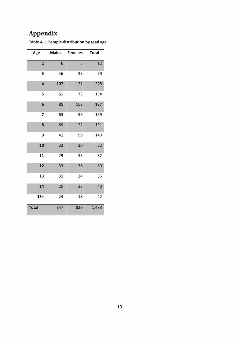
All flounders sampled were measured and weighed. Otoliths were removed, weighed, and measured (using a Leica binocular microscope at 16x-40x magnification). Otoliths were then broken and burned to aid the counting annual growth zones, which was completed with the same Leica binocular microscope as used for otolith measurements. The age distribution according to annual growth zone

3

counts is given in Table A.1 in the appendix. Despite potential problems with age reading quality, we will interpret the read age as true age for the rest of the paper.

Statistical analysis and results The statistical analysis was carried out using Stata IC, version 12 for M.S. Windows. Bhattacharya’s decomposition was implemented using programs provided by Salgado-Ugarte et al. 2000, with modifications by one of us (M.G.). von Bertalanffy growth function was estimated by nonlinear regression using the function evaluator program provided by Salgado-Ugarte et al. 2000. Kernel smoothing and regression analysis was carried out using standard Stata.

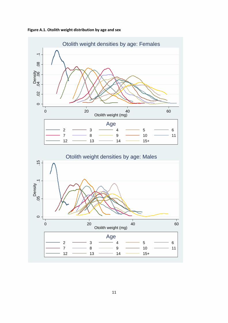
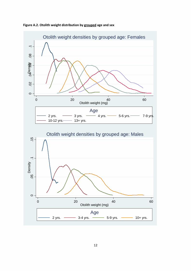
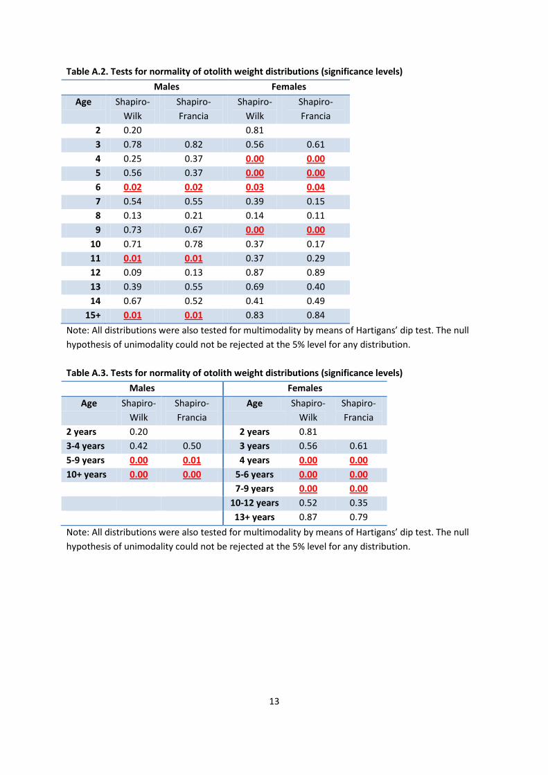
Examination of otolith weight distributions by (read) age First, otolith weight distributions by sex and year class were estimated by kernel densities (using the Epanechnikov kernel with default (optimal) bandwidth). The results (shown in Figure A.1 in the Appendix) showed very poor separation of all but the very lowest year classes for both sexes. To identify separable components, we therefore employed an ad hoc algorithm inspired by hierarchical clustering methods. In each step of the analysis, we computed a separation index for each pair of adjacent group distributions in standard deviation units.1 We then merged the two groups with the lowest separation, recalculated the means and standard deviations, and repeated. The process was terminated when no two groups were separated by less than 0.5 standard deviations. The resulting groups were as follows. For females: 2 years, 3 years, 4 years, 5-6 years, 7-9 years, 10-12 years, and 13+ years. For males: 2 years, 3-4years, 5-9 years, and 10+ years. The resulting densities are shown in the Appendix, Figure A.2. The apparent bimodality in the female year-3 class appears to be due to differences between Subdivisions 26 and 28. However, it should be noted that Hartigan’s (1985) dip test for multimodality fails to reject the null hypothesis of a single mode at 95% significance for any of the distributions. Shapiro-Wilk ad Shapiro-Francia tests do indicate departures from normality for both grouped and ungrouped distributions (Appendix, Tables A.2 and A.3), casting some doubt on the validity of Bhattacharya’s Gaussian decomposition, but given unimodality, these departures should not be too damaging. The fact that higher age groups are harder to separate than lower age groups is due to increasing standard deviations and decreasing increments in means over time (see otolith weight growth curves below). The observed grouping suggests that higher components extracted from the aggregate otolith weight distribution by Bhattacharya’s analysis (see below) are likely to correspond to groups of year classes rather than individual years.

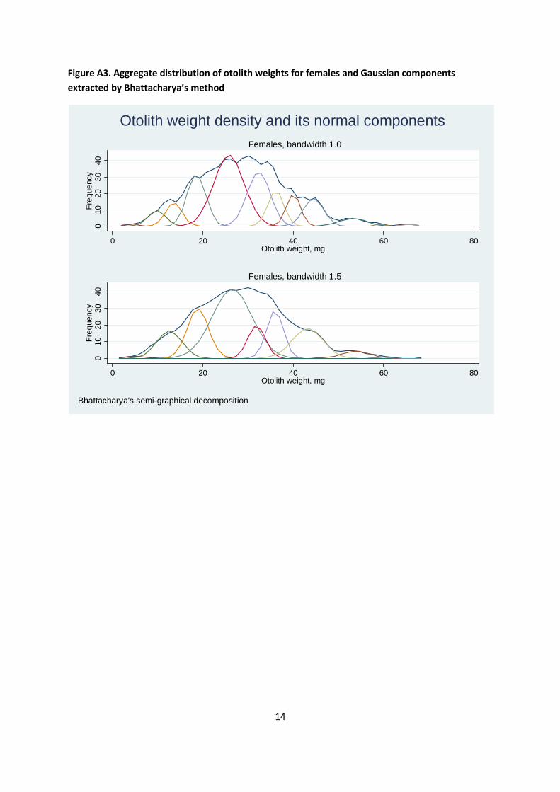
Bhattacharya’s decomposition To estimate the age distribution from otolith weight data alone, we decomposed the aggregate otolith weight distribution (separately for each sex) by Bhattacharya’s semi-graphical method, which is described in detail in Salgado-Ugarte et al. (2000), Sparre and Venema (1992), and Bhattacharya (1967). Prior to the decomposition, the aggregate decomposition was smoothed by Gaussian kernel. After testing a range of kernel bandwidths, two solutions provided the best fit. These were represented by bandwidths 1.0 and 1.5. The two decompositions for females are shown in the

1 If the two distributions had means m1 and m2 and standard deviations s1 and s2, the difference would have mean m=m2-m1 and (assuming independence) standard deviation 𝑠 = �(𝑠1)2 + (𝑠2)2. We define the separation index as m/s.

4

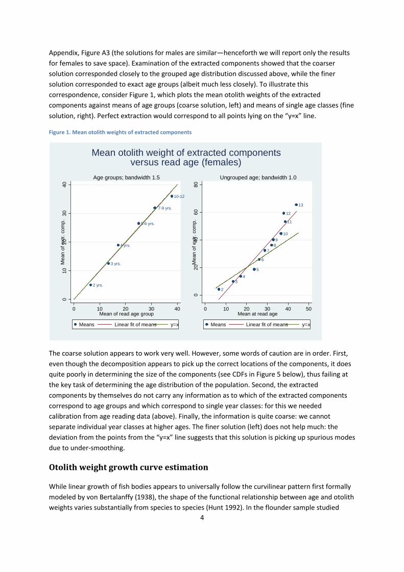
Appendix, Figure A3 (the solutions for males are similar—henceforth we will report only the results for females to save space). Examination of the extracted components showed that the coarser solution corresponded closely to the grouped age distribution discussed above, while the finer solution corresponded to exact age groups (albeit much less closely). To illustrate this correspondence, consider Figure 1, which plots the mean otolith weights of the extracted components against means of age groups (coarse solution, left) and means of single age classes (fine solution, right). Perfect extraction would correspond to all points lying on the “y=x” line.

Figure 1. Mean otolith weights of extracted components

The coarse solution appears to work very well. However, some words of caution are in order. First, even though the decomposition appears to pick up the correct locations of the components, it does quite poorly in determining the size of the components (see CDFs in Figure 5 below), thus failing at the key task of determining the age distribution of the population. Second, the extracted components by themselves do not carry any information as to which of the extracted components correspond to age groups and which correspond to single year classes: for this we needed calibration from age reading data (above). Finally, the information is quite coarse: we cannot separate individual year classes at higher ages. The finer solution (left) does not help much: the deviation from the points from the “y=x” line suggests that this solution is picking up spurious modes due to under-smoothing.

Otolith weight growth curve estimation

While linear growth of fish bodies appears to universally follow the curvilinear pattern first formally modeled by von Bertalanffy (1938), the shape of the functional relationship between age and otolith weights varies substantially from species to species (Hunt 1992). In the flounder sample studied

2 yrs.

3 yrs.

4 yrs.

5-6 yrs.

7-9 yrs.

10-12 yrs.

010

2030

40M

ean

of e

xtr.

com

p.

0 10 20 30 40Mean of read age group

Means Linear fit of means y=x

Age groups; bandwidth 1.5

2

34

5

6

789

10

11

12

13

020

4060

80M

ean

of e

xtr.

com

p.

0 10 20 30 40 50Mean at read age

Means Linear fit of means y=x

Ungrouped age; bandwidth 1.0

Mean otolith weight of extracted componentsversus read age (females)

5

here, however, we observe a clear Bertalanffy growth pattern, which is differentiated by sex. Von Bertalanffy’s equation arises as the general solution to an ordinary differential equation postulating growth that is linearly decreasing in current size. In the case of otolith weights, the ordinary

differential equation becomes 𝑑𝑤𝑡𝑑𝑡

= 𝐾(𝑊∞ −𝑊𝑡), where Wt is otolith weight at time t, 𝑊∞ the

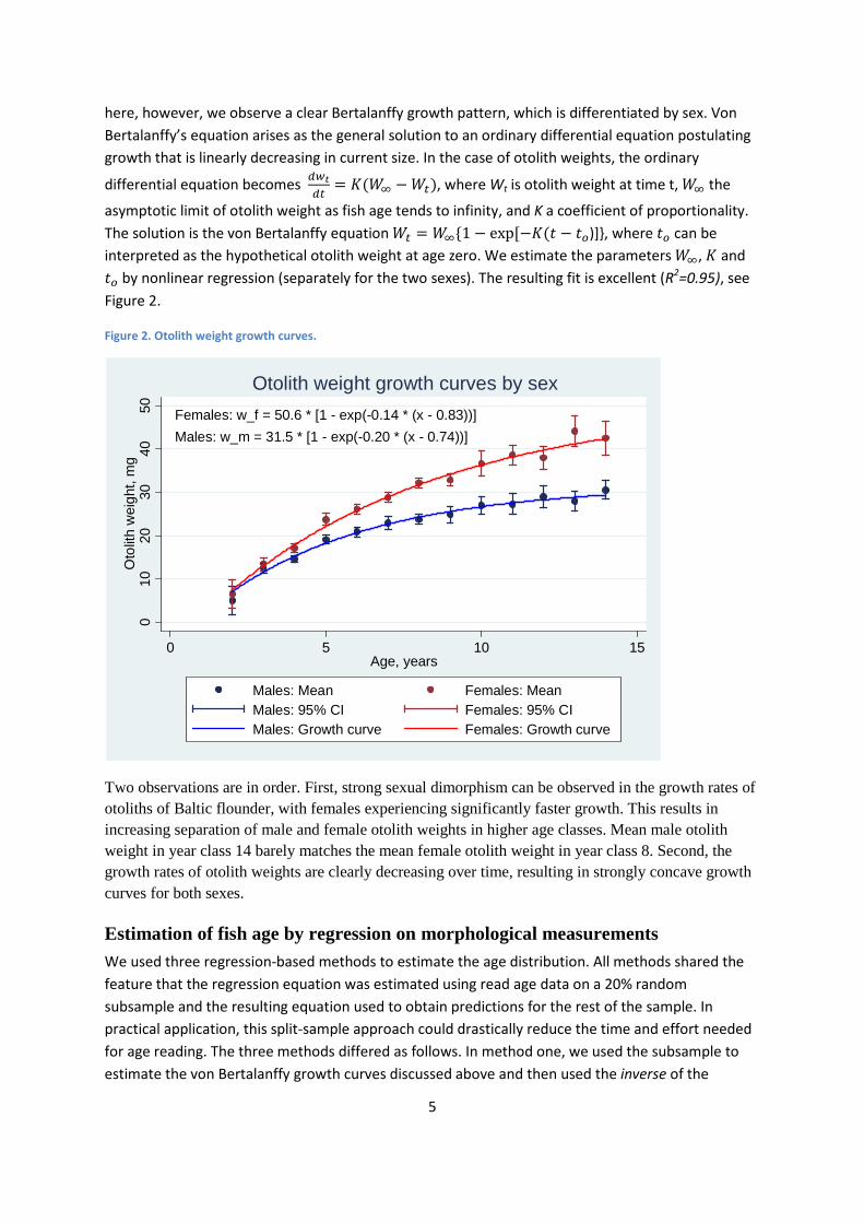
asymptotic limit of otolith weight as fish age tends to infinity, and K a coefficient of proportionality. The solution is the von Bertalanffy equation 𝑊𝑡 = 𝑊∞{1 − exp [−𝐾(𝑡 − 𝑡𝑜)]}, where 𝑡𝑜 can be interpreted as the hypothetical otolith weight at age zero. We estimate the parameters 𝑊∞, 𝐾 and 𝑡𝑜 by nonlinear regression (separately for the two sexes). The resulting fit is excellent (R2=0.95), see Figure 2.

Figure 2. Otolith weight growth curves.

Two observations are in order. First, strong sexual dimorphism can be observed in the growth rates of otoliths of Baltic flounder, with females experiencing significantly faster growth. This results in increasing separation of male and female otolith weights in higher age classes. Mean male otolith weight in year class 14 barely matches the mean female otolith weight in year class 8. Second, the growth rates of otolith weights are clearly decreasing over time, resulting in strongly concave growth curves for both sexes.

Estimation of fish age by regression on morphological measurements We used three regression-based methods to estimate the age distribution. All methods shared the feature that the regression equation was estimated using read age data on a 20% random subsample and the resulting equation used to obtain predictions for the rest of the sample. In practical application, this split-sample approach could drastically reduce the time and effort needed for age reading. The three methods differed as follows. In method one, we used the subsample to estimate the von Bertalanffy growth curves discussed above and then used the inverse of the

Females: w_f = 50.6 * [1 - exp(-0.14 * (x - 0.83))]Males: w_m = 31.5 * [1 - exp(-0.20 * (x - 0.74))]

010

2030

4050

Oto

lith

wei

ght,

mg

0 5 10 15Age, years

Males: Mean Females: MeanMales: 95% CI Females: 95% CIMales: Growth curve Females: Growth curve

Otolith weight growth curves by sex

6

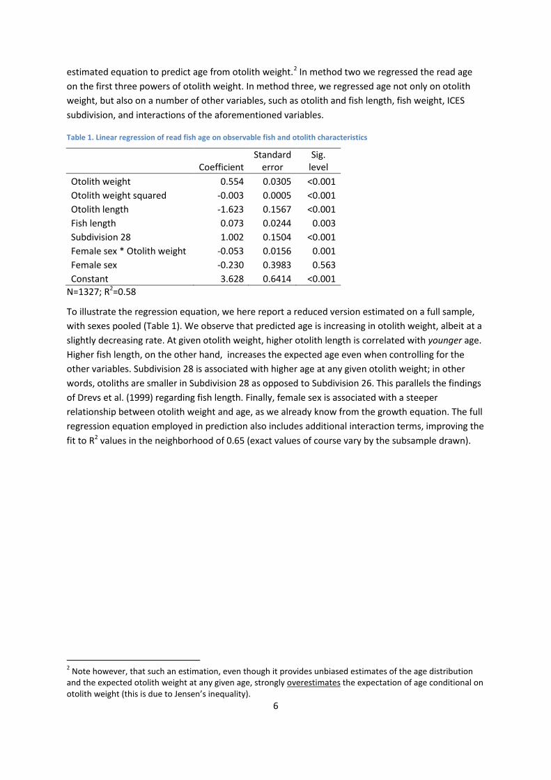
estimated equation to predict age from otolith weight.2 In method two we regressed the read age on the first three powers of otolith weight. In method three, we regressed age not only on otolith weight, but also on a number of other variables, such as otolith and fish length, fish weight, ICES subdivision, and interactions of the aforementioned variables.

Table 1. Linear regression of read fish age on observable fish and otolith characteristics

Coefficient

Standard error

Sig. level

Otolith weight 0.554 0.0305 <0.001 Otolith weight squared -0.003 0.0005 <0.001 Otolith length -1.623 0.1567 <0.001 Fish length 0.073 0.0244 0.003 Subdivision 28 1.002 0.1504 <0.001 Female sex * Otolith weight -0.053 0.0156 0.001 Female sex -0.230 0.3983 0.563 Constant 3.628 0.6414 <0.001

N=1327; R2=0.58

To illustrate the regression equation, we here report a reduced version estimated on a full sample, with sexes pooled (Table 1). We observe that predicted age is increasing in otolith weight, albeit at a slightly decreasing rate. At given otolith weight, higher otolith length is correlated with younger age. Higher fish length, on the other hand, increases the expected age even when controlling for the other variables. Subdivision 28 is associated with higher age at any given otolith weight; in other words, otoliths are smaller in Subdivision 28 as opposed to Subdivision 26. This parallels the findings of Drevs et al. (1999) regarding fish length. Finally, female sex is associated with a steeper relationship between otolith weight and age, as we already know from the growth equation. The full regression equation employed in prediction also includes additional interaction terms, improving the fit to R2 values in the neighborhood of 0.65 (exact values of course vary by the subsample drawn).

2 Note however, that such an estimation, even though it provides unbiased estimates of the age distribution and the expected otolith weight at any given age, strongly overestimates the expectation of age conditional on otolith weight (this is due to Jensen’s inequality).

7

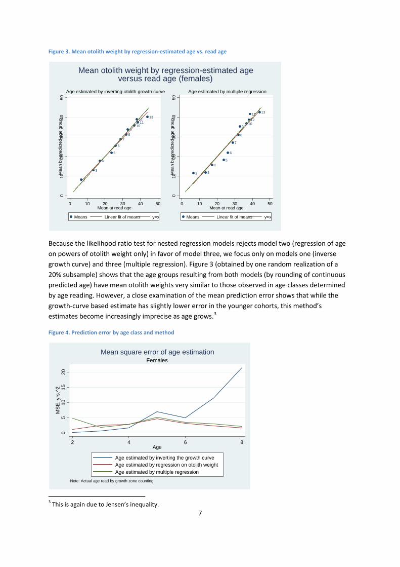
Figure 3. Mean otolith weight by regression-estimated age vs. read age

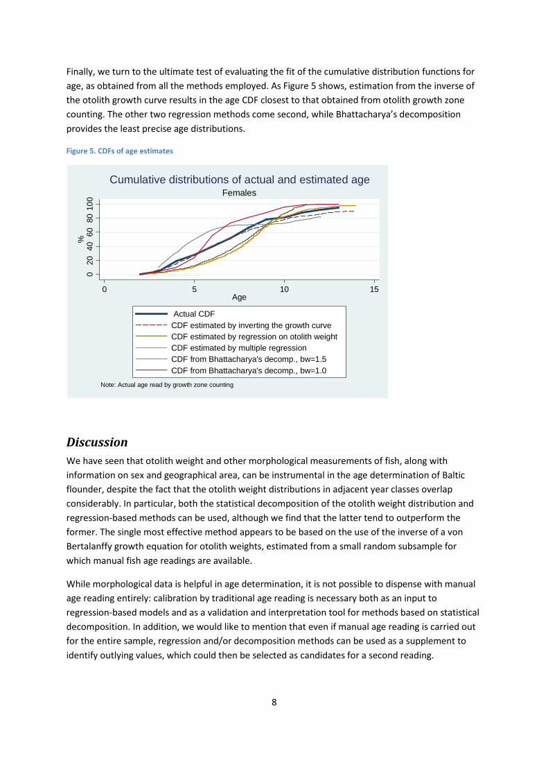
Because the likelihood ratio test for nested regression models rejects model two (regression of age on powers of otolith weight only) in favor of model three, we focus only on models one (inverse growth curve) and three (multiple regression). Figure 3 (obtained by one random realization of a 20% subsample) shows that the age groups resulting from both models (by rounding of continuous predicted age) have mean otolith weights very similar to those observed in age classes determined by age reading. However, a close examination of the mean prediction error shows that while the growth-curve based estimate has slightly lower error in the younger cohorts, this method’s estimates become increasingly imprecise as age grows.3

Figure 4. Prediction error by age class and method

3 This is again due to Jensen’s inequality.

2

3

4

5

6

789

1011

1213

010

2030

4050

Mea

n by

pre

dict

ed a

ge g

roup

0 10 20 30 40 50Mean at read age

Means Linear fit of means y=x

Age estimated by inverting otolith growth curve

2 3

45

6

7

8

910

1112

13

010

2030

4050

Mea

n by

pre

dict

ed a

ge g

roup

0 10 20 30 40 50Mean at read age

Means Linear fit of means y=x

Age estimated by multiple regression

Mean otolith weight by regression-estimated ageversus read age (females)

05

1015

20M

SE

, yrs

.^2

2 4 6 8Age

Age estimated by inverting the growth curveAge estimated by regression on otolith weightAge estimated by multiple regression

Note: Actual age read by growth zone counting

FemalesMean square error of age estimation

8

Finally, we turn to the ultimate test of evaluating the fit of the cumulative distribution functions for age, as obtained from all the methods employed. As Figure 5 shows, estimation from the inverse of the otolith growth curve results in the age CDF closest to that obtained from otolith growth zone counting. The other two regression methods come second, while Bhattacharya’s decomposition provides the least precise age distributions.

Figure 5. CDFs of age estimates

Discussion We have seen that otolith weight and other morphological measurements of fish, along with information on sex and geographical area, can be instrumental in the age determination of Baltic flounder, despite the fact that the otolith weight distributions in adjacent year classes overlap considerably. In particular, both the statistical decomposition of the otolith weight distribution and regression-based methods can be used, although we find that the latter tend to outperform the former. The single most effective method appears to be based on the use of the inverse of a von Bertalanffy growth equation for otolith weights, estimated from a small random subsample for which manual fish age readings are available.

While morphological data is helpful in age determination, it is not possible to dispense with manual age reading entirely: calibration by traditional age reading is necessary both as an input to regression-based models and as a validation and interpretation tool for methods based on statistical decomposition. In addition, we would like to mention that even if manual age reading is carried out for the entire sample, regression and/or decomposition methods can be used as a supplement to identify outlying values, which could then be selected as candidates for a second reading.

020

4060

8010

0%

0 5 10 15Age

Actual CDFCDF estimated by inverting the growth curveCDF estimated by regression on otolith weightCDF estimated by multiple regressionCDF from Bhattacharya's decomp., bw=1.5CDF from Bhattacharya's decomp., bw=1.0

Note: Actual age read by growth zone counting

FemalesCumulative distributions of actual and estimated age

9

References Bhattacharya, C. G. (1967). “A simple method of resolution of a distribution into Gaussian

components”. Biometrics 23: 115–135.

Boehlert, G.W. (1985). “Using objective criteria and multiple regression models for age determination in fishes”. Fishery Bulletin 83: 103–117.

Cardinale, M., and F. Arrhenius. (2004). “Using otolith weight to estimate the age of haddock (Melanogrammus aeglefinus): A tree model application.” Journal of Applied Ichthyology 20: 470–475.

Cardinale, M., F. Arrhenius, and B. Johnsson. (2000). “Potential use of otolith weight for the determination of age-structure of Baltic cod (Gadus morhua) and plaice (Pleuronectes platessa)”. Fisheries Resources 45(3): 239–252.

Drevs, T., and T. Raid. (2010). “Comparative study of three alternative methods of aging Baltic flounder (Platichthys flesus)”. Estonian Journal of Ecology 59( 2): 136–146.–

Drevs, T., V. Kadakas, T. Lang, and S. Mellergaard. (1999). “Geographical variation in the age/ length relationship in Baltic flounder (Platichtys flesus)”. ICES Journal of Marine Science 56: 134–137.

Hartigan, J.A., and P.M. Hartigan. (1985). “The dip test of unimodality”. Annals of Statistics 13(1): 70–84.

Hunt, J. J. (1992). “Morphological characteristics of otoliths for selected fish in the Northwest Atlantic”. Journal of Northwest Atlantic Fishery Science 13: 63–75.

Pilling, G.M. , E.M. Grandcourt, and G.P. Kirkwood. (2003). “The utility of otolith weight as a predictor of age in the emperor Lethrinus mahsena and other tropical fish species.” Fisheries Resources 60(2–3): 493–506.

Pino, C. A., L.A. Cubillos, M. Araya, and A. Sepulveda. ( 2004). “Otolith weight as an estimator of age in the Patagonian grenadier, Macruronus magellanicus, in central-south Chile”. Fisheries Resources 66(2–3): 145–156.

Salgado-Ugarte, I.H., J. Martinez-Ramirez, J. L. Gomez-Marquez, and B. Pena-Mendoza. (2000). “sg128: Some programs for growth estimation in fisheries biology”. Stata Technical Bulletin 53: 35–47.

Sparre, P., and S.C. Venema. (1992). “Introduction to tropical fish stock assessment. Part I.” Manual. FAO, Rome.

von Bertalanffy, L. (1938). “A quantitative theory of organic growth.” Human Biology 10: 181–243.

10

Appendix Table A.1. Sample distribution by read age

Age Males Females Total

2 6 6 12

3 46 33 79

4 107 121 228

5 61 73 134

6 85 102 187

7 63 96 159

8 69 122 191

9 41 99 140

10 32 30 62

11 29 53 82

12 33 36 69

13 31 24 55

14 20 23 43

15+ 24 18 42

Total 647 836 1,483

11

Figure A.1. Otolith weight distribution by age and sex

0.0

2.0

4.0

6.0

8.1

Den

sity

0 20 40 60Otolith weight (mg)

2 3 4 5 6 7 8 9 10 11 12 13 14 15+

Age

Otolith weight densities by age: Females0

.05

.1.1

5D

ensi

ty

0 20 40 60Otolith weight (mg)

2 3 4 5 6 7 8 9 10 11 12 13 14 15+

Age

Otolith weight densities by age: Males

12

Figure A.2. Otolith weight distribution by grouped age and sex

0.0

2.0

4.0

6.0

8.1

Den

sity

0 20 40 60Otolith weight (mg)

2 yrs. 3 yrs. 4 yrs. 5-6 yrs. 7-9 yrs. 10-12 yrs. 13+ yrs.

Age

Otolith weight densities by grouped age: Females0

.05

.1.1

5D

ensi

ty

0 20 40 60Otolith weight (mg)

2 yrs. 3-4 yrs. 5-9 yrs. 10+ yrs.Age

Otolith weight densities by grouped age: Males

13

Table A.2. Tests for normality of otolith weight distributions (significance levels) Males Females

Age Shapiro-Wilk

Shapiro- Francia

Shapiro-Wilk

Shapiro- Francia

2 0.20 0.81 3 0.78 0.82 0.56 0.61 4 0.25 0.37 0.00 0.00 5 0.56 0.37 0.00 0.00 6 0.02 0.02 0.03 0.04 7 0.54 0.55 0.39 0.15 8 0.13 0.21 0.14 0.11 9 0.73 0.67 0.00 0.00

10 0.71 0.78 0.37 0.17 11 0.01 0.01 0.37 0.29 12 0.09 0.13 0.87 0.89 13 0.39 0.55 0.69 0.40 14 0.67 0.52 0.41 0.49

15+ 0.01 0.01 0.83 0.84 Note: All distributions were also tested for multimodality by means of Hartigans’ dip test. The null hypothesis of unimodality could not be rejected at the 5% level for any distribution. Table A.3. Tests for normality of otolith weight distributions (significance levels)

Males Females Age Shapiro-

Wilk Shapiro- Francia

Age Shapiro-Wilk

Shapiro- Francia

2 years 0.20 2 years 0.81 3-4 years 0.42 0.50 3 years 0.56 0.61 5-9 years 0.00 0.01 4 years 0.00 0.00 10+ years 0.00 0.00 5-6 years 0.00 0.00 7-9 years 0.00 0.00 10-12 years 0.52 0.35 13+ years 0.87 0.79 Note: All distributions were also tested for multimodality by means of Hartigans’ dip test. The null hypothesis of unimodality could not be rejected at the 5% level for any distribution.

14

Figure A3. Aggregate distribution of otolith weights for females and Gaussian components extracted by Bhattacharya’s method

010

2030

40Fr

eque

ncy

0 20 40 60 80Otolith weight, mg

Females, bandwidth 1.0

010

2030

40Fr

eque

ncy

0 20 40 60 80Otolith weight, mg

Females, bandwidth 1.5

Bhattacharya's semi-graphical decomposition

Otolith weight density and its normal components