Vol. 12(3), pp. 130-141, July-September 2020

DOI: 10.5897/JEIF2020.1062

Article Number: 8C78D9864747

ISSN 2006-9812

Copyright©2020

Author(s) retain the copyright of this article

http://www.academicjournals.org/JEIF

Journal of Economics and International Finance

Full Length Research

Two qualified models of learning by doing

Samuel Huhui

Transportation Bureau of Shenzhen Municipal, China.

Received 29 June, 2020; Accepted 29 July, 2020

Learning by doing (or learning curves) is a well-known law in economics and psychology, but no consensus has been achieved on the “qualified” models for more than a century. This article explores the expression of learning by doing in a way where the expression is not involved with changing the prime factors of a learning process. If one prime factor changes dramatically during the course of a learning process, the result of the regression is actually an approach to link two different learning curves. If the two curves are distinguishable, they each obey the law of learning by doing, which will progress rapidly at the initial phase and gradually slow down to a flat end. This article presents two functions as the law of learning by doing: The general exponential model is 0.79:0.21 better than the exponential delay model, whereas the later has the ability to investigate the change of loading factors. This ability makes the models a powerful tool for entrepreneurs and managers in investment and production planning. Key words: Learning by doing, function expression, single equation models, firm behavior, empirical analysis.

INTRODUCTION The law of the learning curves has become ubiquitous since its introduction in an 1885 study of individuals in psychology, and has been found in the manufacturing process of industrial organizations, called ―learning by doing‖ or ―organizational learning‖ in the field of economics and management (Wright, 1936). Empirical evidence of more than thousands of industries such as aircraft assembly, ship building by big firms, as well as cigar making by small firms have shown this law being used in industries broadly (Yelle, 1979; Thompson, 2010; Anzanello and Fogliatto, 2011; Jaber, 2016). The core idea of the law of the learning curves is negative acceleration: as one practices and learns more in a specific domain, the amount of unknown material decreases and, thus, the amount of newly learned information declines. Therefore, it is natural to anticipate

progress being essentially null at the end of the learning process, which Bryan and Harter (1897, 1899) termed the ―plateau.‖

However, this explanation is assumed to be insufficient, as the learning process has long been reported as continuing infinitely with no convincing evidence of an end in progress (Wright, 1936; Jaber, 2016; Hirschmann, 1964; Dar-El et al., 1995; Asher, 1956). For example, Arrow (1962) seminal work was based on the log-linear function y = px

r

of Wright (1936), who found that when the

output doubled, the cost of airplane declined along the power sequence infinitely to 0. Although this finding was and is counterintuitive, that the cost of airplane should be much higher than 0, a vast body of empirical evidence supports that the end of learning process is ambiguous. Recently, this phenomenon was partly attributed to the

E-mail: hhsamuel@aliyun.com.

Author(s) agree that this article remain permanently open access under the terms of the Creative Commons Attribution

License 4.0 International License

Huhui 131

Table 1. Models.

Name Function expression Value range of parameter Monotonicity

Exp-Gen1 1xy k pr 0, 0,0 1k p r Decrease

Exp-Delay ( 1) / ( )xry k p t t e 0, 0, 0, 0k p t r Decrease

Stanford-B ( )ry p x t 0, 0, 1 0p t r Decrease

S-curve 1[ (1 )( ) ]ry c M M x t 1 0,0 1, 0, 1 0c m t r Decrease

Log-Linear ry px 0, 1 0p r Decrease

DeJong 1[ (1 ) ]ry c M M x 1 0,0 1, 1 0c m r Decrease

Power-Delay ( 1) / ( )ry k p t t x 0, 0, 0, 0k p t r Decrease

Power-Gen ry k px

0, 0, 1 0k p r Decrease

Hyp2 [ / ( )]y k x x r 0, 0k r Increase

Exp2 /(1 )x ry k e 0, 0k r Increase

Exp3 ( )/(1 )x p ry k e 0, 0, 0k p r Increase

Hyp3 ( ) / ( )y k x p x p r 0, 0, 0k p r Increase 1 The originators of models are listed as follows: Exp-Gen (Pegels, 1969; Towill, 1990); Exp-Delay (Evans et al. 2018); Stanford-B

(Asher, 1956); S-curve (Carr, 1946); Log-liner (Wright 1936); DeJong (De Jong, 1957); Power-Delay (Evans et al., 2018); Power-Gen (Newell and Rosenbloom 1981); the rest four models Hyp2, Exp2, Hyp3, Exp3 originated by Mazur and Hastie (1978) and Nembhard and Uzumeri (2000).

―leaps‖ (Gray, 2017; Gray and Lindstedt, 2017). Slow progress followed by rapid learning in the initial phase has also been long discussed, and was termed as ―initial delay‖ (Carr, 1946; Evans et al., 2018). To achieve a better fit with all of the divergent empirical datasets, scholars have introduced more than a dozen learning curve models (Table 1), and constant efforts have been made to determine which is best (Crossman, 1959; Nembhard and Uzumeri, 2000; Newell and Rosenbloom, 1981; Badiru, 1992; Heathcote et al., 2000; Anzanello and Fogliatto, 2011; Evans et al., 2018). However, different models better fit different datasets, and no consensus has been achieved on ―qualified‖ models.

This study aims to identify reasonable and qualified models of ―learning by doing‖ by illuminating the mechanism of the learning process. The key idea in this study is that the process of learning is compounded by different factors and that performance improvement is actually the improvement of loading factors, meaning there are two methods for learning to progress: improve the performance of loading factors and reload more efficient factors. A learning model can be applied only under the condition that the prime factors of a learning process do not change dramatically. The law of the learning curve should be discussed apart from how to significantly change the prime factors of current manufacturing processes. If one prime factor changes dramatically during the course of a learning process, the result of the regression is actually an approach to link two different learning curves. If the two curves are distinguishable, they each obey the law of learning by

doing, which will progress rapidly at the initial phase and gradually slow down to achieve plateau (Bryan and Harter, 1897, 1899). The plateau indicates a time when the prime factors of a learning process have approached their limits until a change of prime factors occurs.

To illustrate this idea, this article uses empirical evidence of organizational learning in railway industry, which also illustrates that the controversial phenomena of the ―leap‖ (Teplitz, 2014; Gray, 2017; Gray and Lindstedt, 2017) and ―initial delay‖ (Evans et al., 2018) are both the result of the change in prime factors.

For any theory, nothing is more important than determining the accurate function expression because it not only articulates the relationship between variables but also unveils the mechanism behind this relationship, and thus, explains that why a microeconomic law can be used in macroeconomics. For the empirical evidence of the Shenzhen railway industry, the general exponential model (presented by Pegels 1969; Towill 1990 in different forms

1) is the best, at 0.79:0.21; it performs better than

the exponential delay model (Evans et al., 2018), although the exponential delay model has some ability to detect changes in loading factors. The two functions can

1 According to Towill (1990), /y (1 )x t

c fy y e /y ( ) x t

c f fy y y e , denote ( )c fk y y ,

1/t

fp y e , 1/tr e , then,

1xy k pr .

132 J. Econ. Int. Finance not only predict the future performance of an organization but also distinguish eligible datasets from ineligible ones. This ability makes the models a powerful tool for entrepreneurs and managers in investment and production planning, as well as researchers. Background and models When an individual learns a skill, he or she usually experiences a period of rapid improvement in performance followed by a period without obvious progress and then more improvement. This period with no obvious progress is called a plateau on the learning curve. Bryan and Harter (1897, 1899) were the first to describe the limit of learning as a ―plateau‖ after studying individuals’ skills in receiving Morse code and finding a steady state without obvious progress between one rapid period of improvement and another period of improvement. They believed this plateau was because learning involves a hierarchy of habits, in which (using Morse code as an example) letters must be learned first, followed by the sequences of letters forming syllables and words, and finally phrases and sentences. A plateau is a point of transition, when lower-order habits are not sufficiently learned to advance to the next level of habits in the hierarchy; thus, the pace of progress slows until this lower-order learning is completed. This notion prevailed until the Second World War. Half a century after Bryan and Harter, the speed of sending and receiving Morse code improved greatly and researchers found little difference between receiving sentences, unrelated words, nonsense material, and random letters—unexpected from the hypothesis of a hierarchy of habits. Most importantly, the anticipated plateaus did not appear (Keller, 1958).

Wright's (1936) log-linear model is another example of the ―phantom‖ plateau. Asher (1956) assumed this was because the period of observation was not long enough and, thus, presented the Stanford-B model. In this model, despite that cost of aircraft declining significantly toward 0 with no observable signs of plateau, Asher insisted that the learning progress would slow down in the long run while it remains infinite and ends ambiguously. De Jong (1957) is perhaps the only writer to outline why the learning curve should have a limit, explaining that because learning was a characteristic of human beings and machines could not learn, manufacturing had an ―incompressibility‖ factor. Soon after, Crossman (1959) provided cases demonstrating these incompressibility factors, most notably the cycle time of a cigar-making firm. During the startup phase, cycle time declined along the Log-Linear curve, but two years later, the Log-Linear curve bent to a lower limit. Crossman (1959) believed this lower limit demonstrated the machinery’s incompressibility factor. However, subsequent studies (Hirschmann, 1964) implied the ―machine factor‖ should not lead to a plateau because if the machine is the

incompressibility factor, then operations paced by people should have steeper slopes than those paced by machines-that is, the less human involvement, the less capacity for learning. As an example, the petroleum industry was characterized by large investments in heavy equipment and so highly automated that learning was thought to be either non-existent or of insignificant value. However, the empirical evidence found the progress ratio in cost per barrel of capacity from 1942 to 1958 was almost the same as many other industries fitting the assumption that the limit is 0, as well as the average direct person-hours per barrel from 1888 to 1962, and that this also held true in the electric power and steel industries, and so on. Dar-El et al. (1995) stated frankly that even in the long run, there is no scientific work supporting the assumption of DeJong and Crossman.

The mainstream of contemporary studies on the law of learning curve is to test the hierarchy hypothesis (Gray, 2017; Gray and Lindstedt, 2017; Evans et al., 2018). However, as Jaber (2016) states, there is no tangible consensus among researchers as to what causes a plateau in the learning curve.

This article investigates 12 models that are most often cited in the literature (Table 1). Some letters of the variables differ from the original literature, they are unified here according to the meaning of the variables. For all models listed in Table 1, parameter k is the asymptote for performance after an infinite amount of practice without random impact by external variables, p concerns the working group’s experience before manufacturing, (which is usually defined as the person-hours needed for the first product), and r is the learning rate in functions. Although parameters k, p, and r roughly mean the same thing in all models, they are different in their range of value.

These 12 models can be divided into two types: the first involves y decreasing continuously with the increase of x (eight models), and the second involves y increasing with the increase of x (four models), and actually, they mean the same. For example, in the general exponential model (Towill, 1990; Pegels, 1969), y is the person-hours needed to produce a product, which declines with the increase in production number; that is, more products x being produced means fewer person-hours are needed for the x-th unit. By contrast, in the Hyp2 model (Mazur and Hastie, 1978; Nembhard and Uzumeri, 2000), y is the number of products produced in one unit of time, which increases with the increase in time x spent on production.

The essential divergence among these models lies in two questions: First, which does it assume, plateau or leap? Second, does it allow for a slow start-up phase? As a reflection of the controversy, the most popular models among scholars (Log-Linear, Stanford-B) simply do not have asymptote because they sometimes fit even better. Moreover, asymptote is allowed to be 0 in decreasing models or can be quite large in the increasing models. To provide a reasonable explanation of the plateau, the

special parameter M (DeJong, S-curve) was created to incorporate the influence of machinery. In terms of the start-up phrase, four models (Exp-Delay, Power-Delay, Stanford-B, S-curve) indicate the degree of delay for the start-up phrase with parameter t; in the initial delay models, the learning process is not rapid at the beginning but progress is instead rapid after a period of learning initiation, when t does not equal 0. K, p, r and M, t are the parameters employed in this study. Theory When we observe organizational learning in manufacturing, we can easily divide the production process into numerous small factors. For example, Asher (1956) divided the total person-hours in aircraft assembly into 10 major procedures (e.g., final assembly, fuselage major assembly, and miscellaneous sub-assembly); the cost of these procedures could be improved independently or further divided, with the total cost of the product being the sum of the costs of its factors. Along with the improvement of every loading factor, this presents another method to accelerate the learning curve: load more efficient factors by replacing, or without replacing, the original factors. For example, when the numerically controlled machines in a flat-screen television manufacturing procedure were replaced by a ―smarter‖ computer numerically controlled machine, the product cost per unit reduced considerably, which is a ―leap‖ (Teplitz, 2014; Gray, 2017; Gray and Lindstedt, 2017). Thus, academics have intuitively accepted these two methods for the learning curve to progress.

The key difference that separates this study from previous ones is that the studies allowed for these two progression methods to converge and did not distinguish between them. By contrast, this study emphasizes that a learning model should be used strictly under the condition that all factors remain unchanged in theory or, in practice, the prime factor(s) should at least not change dramatically. The reason to hold all factors of a learning process unchanged is that when factors change, they could also turn the learning process into an entirely different procedure, thus making the regression meaningless. For example, one feature of the pre-2012 railway industry in Shenzhen was that it mainly used traditional diesel locomotives; however, in January 2012, the new high-speed railway came into service with electric locomotives. Using the industry transition of two learning processes would be unsuitable, as it involves two types of trains belonging to many different railway companies on two types of railways using two different techniques.

However, if this requirement of factors remaining unchanged is followed strictly, no eligible datasets would be found as factors constantly change in every learning process. Furthermore, the train system is an aggregation

Huhui 133 of all trains and stations; train service using one electric locomotive between two stations does not change the prime factor of the large system, and it is hard to draw a rigid theoretical line as to how many added electric locomotives and stations exactly brings about the change in prime factors. Arguing that prime factors should not change dramatically is a compromise, but that does not mean ―dramatically‖ is ambiguous. In this case, a dramatic change means heavy investment in new infrastructure and facilities in comparison to previous investments, as well as hard work that differs from previous efforts by entrepreneurs and managers. It should not be hard for entrepreneurs and managers to distinguish the prime factors because they cause a dramatic change of prime factors to occur.

The process of forgetting (Benkard, 2000; Jaber, 2006) should be excluded for the same reason, as it is a process of constantly losing loading factors and not of ―learning.‖ The desired condition of a learning process is that one should deliberately practice (Ericsson et al., 1993) to improve ability with the exclusion of dramatic changes to prime loading factors.

The general exponential model (Pegels, 1969; Towill, 1990) and the exponential delay model (Evans et al., 2018) fit the data well and predict the plateau in performance, and the fact that they fit so well in difficult conditions means the need for a new model is not urgent. The two models are presented together because they substantively have the same meaning when t=0:

'y ' '( 1) / ( )xrk p t t e ='' ' xrk p e ,

Denote 'k k ,1'p p r , ' lnr r ,

Then

1xy k pr

The relative learning rates (RLR) of the two are

theoretically equal as well because ' lnr r .

( 1)exp

exp

( ) ( )ln ( )

xgen

gen

y k prr y k

x x

, 0<r<1;

'exp

exp

[ ] [ ' '( 1) / ( )]'( ')

xrdelay

delay

y k p t t er y k

x x

, ' 0r .

Thus, for a given dataset with t=0, the general exponential model and the exponential delay model should theoretically progress at a constant RLR ratio along the regression curves.

METHODOLOGY

To refine the qualified models, the factor analysis method was applied to distinguish eligible datasets from ineligible ones in the Shenzhen railway industry database; then, nonlinear regression method was employed (Bates and Watts, 1988) to obtain the value

134 J. Econ. Int. Finance of parameters (k, p, r, t, M), the determination coefficient (R

2), and

the residual sum of squares (RSS). This was followed by an estimation of the reasonable limits of plateaus for the datasets; each was compared with the regressed result of asymptotes (parameter k), and only two models (Exp-Delay, Power-Delay) do not have unreasonable asymptotes across all datasets. Finally, the two models were compared using the Akaike Information Criterion Test (AIC, Akaike 1974), the Bayesian Information Criterion Test (BIC, Schwarz, 1978), and F-test. For calculation, the software Origin 9.1 by OriginLab was used.

The most important task, which missed in previous literature, was to find datasets in the Shenzhen railway transportation industry that met the requirement of prime factors not changing dramatically with the knowledge that factors in transportation change rapidly. On the demand side, every trip is an individual decision triggered by different reasons (an accident in a distant hometown, for example, could necessitate an emergency trip); the most significant regular reason for changes in demand side are the Spring Festival of the Chinese New Year and the peak summer season. The Spring Festival sometimes comes in January and sometimes in February, and it causes a surge in passenger volume before this number drops dramatically; the summer peak comes in June, July, and August as the result of summer vacations. On the supply side, a train can add or cancel a stop without explanation, and arbitrary decisions on the frequency of trains at stations make the data of many stations change substantially. Competition from other modes of transportation (that is by airplane or by automobile) is one of the external factors that significantly influence the number of railway trips, as well as the number and type of residents in Shenzhen. Thus, regression on the railway system is set to be in difficult conditions because different kinds of factors cannot be controlled simultaneously.

Factor analysis focuses on using the supply side to identify different prime factors in a learning process. For example, the two modes of railway transportation (the traditional diesel railway system and the high-speed electric railway system) should be regressed separately; one can also apply regression together beginning with the day the two modes were both in service but not from the beginning of the traditional railway system and over the change to the two modes together. For data involving no change in the railway system type, I observed the yearly increasing rate of trips in every month to identify the prime factors to avoid the seasonal influence on the demand side. The yearly increasing rate in number of trips is assumed to be high at the start-up phase and gradually approach 0, and a significant increase would indicate that a new prime factor has been loaded.

The criterion between eligible and ineligible datasets in this study depends on four requirements, and if one of them was not met, the dataset is ineligible. First, the station or a group of stations should be in service in December 2018. Second, they should have remained in service for at least 12 successive months from the first month of operation to December 2018, and null datum during this period was not allowed. Third, the data demonstrates general growth and not decline. Finally, if the Exp-Delay model fits, the delay parameter t should equal 0. It must be noted that as long as t did not equal 0, the dataset was excluded despite the goodness of fit because it indicated a change in prime factors (which the next section explains; also see Evans et al. (2018), for the connotation of t).

The work of nonlinear curve fitting follows the doctrine articulated by Bates and Watts (1988). According to the Gauss-Newton

method, for equation ,( )y f x , the aim is to find the

expectation value

^

of with the minimum least square value in

2 2

1 1

( ) [ ( , )]n n

i i i

i i

S y f x

. With the expansion in a

first-order Taylor series about , an iterative equation can be

deduced, and the convergence of

^

can be obtained until the

increment of θ is small to the point there is no useful change in the elements of the parameter vector. The convergence criterion in this study is less than 1E-9.

The idea behind plateau estimation is that a given amount of investment in railway system cannot achieve infinite passenger handling capability. The criterion of current plateau presented in this study is less than three times that of the passenger departure volume (PDV) in the highest month of 2018, the regressed asymptote of a model higher than this volume will be unreasonable. Because, the triple PDV by train in a month will be much higher than the number of residents in Shenzhen. The reason for holding the same plateau criterion as Shenzhen’s total volume for the remainder of the eligible datasets is that these datasets are subsets of the total volume and their volume distribution reflects a balanced response to all types of demand for different destinations. No more or less models can be presented in spite of the change of plateau criterion.

To compare the goodness of fit of the two models, I used the AIC (Akaike, 1974), BIC (Schwarz, 1978), and F-test, with the results being the same for the three methods. The reason that only the AIC result is presented is that it tells not only which model is better but also how much the better as a percentage with the information of Akaike’s weight.

Datasets

Railway system data were deliberately selected for this article for two key reasons: They quantify factors and sub-factors in the learning process, and there are two obvious types of learning processes. The data were extracted from two financial settlement system databases of a listed company on the Hong Kong Stock Exchange and the New York Stock Exchange covering January 2007 to December 2018 (so, no data in 2019 are used). They exclude the ticket price and only concern the PDV of railway stations in Shenzhen, a city located in South China that is adjacent to Hong Kong that has the country’s highest per capita gross domestic product. The search found 21 datasets, two being ineligible but illustrated for the phenomenon of leap and initial delay and the remaining 19 being eligible to find the most suitable models. Table 2 provides information from the datasets and the regressed result of mean R

2 of the 12 models for every eligible

datasets. The most notable characteristic of the datasets is that the prime

factors of learning processes can be precisely divided and evaluated, meaning it is essential to know the relationships among the datasets. This is evident from their names, dataset which comprise two or three parts: the first part is an abbreviation of a company and the final part is the initial month of the duration of the dataset, which indicates the PDV of railway station(s) this company charges for in the period under review. For example, China Railway Guangzhou Group (CRGG) is the parent company of all railway station companies in Shenzhen, so the dataset name ―CRGG2007‖ means the PDV of all stations in Shenzhen from January 2007 to December 2018. GuangShen Railway (GSR) is the largest traditional railway company, and ―GSR2007‖ means the monthly PDV from January 2007 to December 2018 in traditional service. ―PH2016oct‖ means the PDV of PH station (a small traditional railway station) from October 2016 to December 2018.

Shenzhen North Station (SNS) is one of the high-speed railway stations and the largest station of CRGG. To investigate the learning phenomenon for the high-speed railway service in detail, an abbreviation of destination station is added as the middle part of

Huhui 135

Table 2. Datasets and the result of determinant coefficient.

Datasets N Unit Mean Variance R2

CRGG2007 144 Million 3.4602 3.5560 ---

SNS2012 84 Million 2.2478 1.6232 ---

GSR2007 144 Million 1.7509 0.0870 0.3368

CRGG2014 60 Million 6.3425 1.0862 0.5408

SNS2014 60 Million 2.9107 0.6174 0.7785

PH2016oct 27 10 thousand 7.2059 1.4739 0.5331

SNS-north-2012 84 Million 1.3092 0.3840 0.8207

SNS-east-2014 60 Million 1.3141 0.1356 0.7899

SNS-FJ-2014 60 100 thousand 5.4646 1.3233 0.4506

SNS-GX-2014dec 49 100 thousand 1.0725 0.1720 0.6791

SNS-HN-2012sep 76 10 thousand 3.3337 2.1454 0.7182

SNS-east-GD-2014 60 100 thousand 11.9838 43.0249 0.8819

SNS-qs-2012 84 Thousand 10.6594 49.0885 0.6126

SNS-ydx-2012apr 81 Thousand 4.8709 4.3452 0.6236

SNS-cs-2014 60 10 thousand 14.3862 19.3061 0.7597

SNS-cy-2014 60 10 thousand 5.3060 3.2241 0.7831

SNS-hm-2014 60 Thousand 9.0724 22.3320 0.8582

SNS-hd-2014 60 Thousand 20.3145 123.9908 0.6770

SNS-hzn-2014 60 10 thousand 9.4233 23.1925 0.7377

SNS-pn-2014 60 10 thousand 9.8543 10.6039 0.7927

SNS-sw-2014 60 10 thousand 6.2335 5.4849 0.8972

the name beginning with SNS concern the monthly PDV from SNS to different destinations. That is, the -north- and -east- means the two high-speed railway systems respectively, the uppercase letters mean a group of stations in a province out of Guangdong, the lowercase letters mean a certain station inside Guangdong province, the province Shenzhen located in.

Data were deleted in these 21 datasets under two conditions: the deleted datum must be the first number of a dataset’s sequence, and it must be significantly smaller than the second month. When the two conditions were met, I checked the first operational day of this railway line and found, without exception, that the PDV in that month was in the trial operation stage and not fully operational for the entire month. In all, 12 numbers in the 21 datasets (1493 numbers in total) are deleted.

RESULTS AND DISCUSSION The influence of newly added factors: Leap and initial delay

Findings show that the change of prime factors causes a systematic leap in the learning process, the intuitive impression that the learning process can go infinitely without plateau overlooks the significant changes in prime factors; this can be illustrated either intuitively by figure or numerically by quantity.

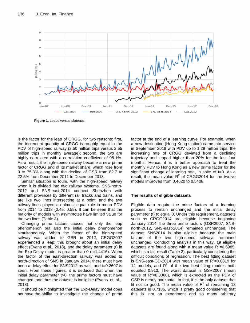
Seeing the PDV of CRGG in Figure 1, an intuitive impression is drawn where CRGG increases from 2007 to 2018 infinitely with no sign of plateau, which is a very similar pattern to the findings of Wright (1936) or Keller

(1958). However, when examining the prime factors (GSR, SNS), the curves show that GSR had plateaued before 2012, whereas SNS, which came into service in 2012, increases infinitely and has a similar pattern like Wright (1936) or Keller (1958) as well. When investigating the prime factors of SNS using the north and east railway lines both came into service for different provinces in 2012 and 2014 respectively the curves show that these two factors also plateaued. As Figure 1 demonstrates, the three railway lines (GSR2007, SNS-north-2012, SNS-east-2014) plateau at a similar volume under the premise that their respective prime factors will not change further. In other words, every learning process will plateau, and the aggregation of the different prime factors that came into service at different times makes the curve rise infinitely.

The conclusion also can be drawn in a numerical way. The asymptote regression results of all models to CRGG2007 are infinite, and the asymptote of SNS2012 is either non-existent or extremely huge (Table 3), which indicates the need to proceed carefully to the existence of a plateau.

However, in the Shenzhen railway system, it is clear that the irregular addition of new prime factors causes the continual leap of PDV as old prime factors plateaued one by one. First of all, for the solo prime factor of CRGG before 2012 (with the market share at 82.7%), GSR has a limited asymptote value in all models, except the two without asymptote (Table 3). Also, the high-speed railway

136 J. Econ. Int. Finance

Figure 1. Leaps versus plateaus.

is the factor for the leap of CRGG, for two reasons: first, the increment quantity of CRGG is roughly equal to the PDV of high-speed railway (2.50 million trips versus 2.55 million trips in monthly average); second, the two are highly correlated with a correlation coefficient of 98.1%. As a result, the high-speed railway became a new prime factor of CRGG and of its market share, which rose from 0 to 75.3% along with the decline of GSR from 82.7 to 22.5% from December 2011 to December 2018.

Similar situation is found with the high-speed railway when it is divided into two railway systems. SNS-north-2012 and SNS-east-2014 connect Shenzhen with different provinces by different rail tracks and trains, and are like two lines intersecting at a point, and the two railway lines played an almost equal role in mean PDV from 2014 to 2018 (0.45: 0.55). It can be seen that the majority of models with asymptotes have limited value for the two lines (Table 3).

Changing prime factors causes not only the leap phenomenon but also the initial delay phenomenon simultaneously. When the factor of the high-speed railway was added to GSR in 2012, CRGG2007 experienced a leap; this brought about an initial delay effect (Evans et al., 2018), and the delay parameter (t) in the Exp-Delay model is greater than 0 (t=1.4416). When the factor of the east-direction railway was added to north-direction of SNS in January 2014, there must have been a delay effect for SNS2012 as well, and t=0.2697 is seen. From these figures, it is deduced that when the initial delay parameter t>0, the prime factors must have changed, and thus the dataset is ineligible (Evans et al., 2018).

It should be highlighted that the Exp-Delay model does not have the ability to investigate the change of prime

factor at the end of a learning curve. For example, when a new destination (Hong Kong station) came into service in September 2018 with PDV up to 1.29 million trips, the increasing rate of CRGG deviated from a declining trajectory and leaped higher than 20% for the last four months. Hence, it is a better approach to treat the monthly PDV to Hong Kong as a new prime factor for the significant change of learning rate, in spite of t=0. As a result, the mean value R

2 of CRGG2014 for the twelve

models improved from 0.4620 to 0.5408. The results of eligible datasets Eligible data require the prime factors of a learning process to remain unchanged and the initial delay parameter (t) to equal 0. Under this requirement, datasets such as CRGG2014 are eligible because beginning January 2014; the three prime factors (GSR2007, SNS-north-2012, SNS-east-2014) remained unchanged. The dataset SNS2014 is also eligible because the main factors of the two high-speed railways remained unchanged. Conducting analysis in this way, 19 eligible datasets are found along with a mean value R

2=0.6985,

which is a fair result (Table 2), particularly considering the difficult conditions of regression. The best fitting dataset is SNS-east-GD-2014 with mean value of R

2=0.8819 for

12 models; and R2 of the two best-fitting models both

equaled 0.913. The worst dataset is GSR2007 (mean value of R

2=0.3368), which is expected as the PDV of

GSR is nearly horizontal. In fact, it is the only dataset that fit not so good. The mean value of R

2 of remaining 18

datasets is 0.7186, which is pretty good considering that this is not an experiment and so many arbitrary

Huhui 137 Table 3. The predicted asymptote of 2 ineligible datasets and 19 eligible datasets comparing with their plateau (ov: over parameterized).

Data sets MAX*3 Unit(trips) Exp-Gen Exp-Delay Stanford-B S-curve Log-Linear DeJong Power-Delay Power-Gen Hyp2 Exp2 Exp3 Hyp3

CRGG2007 - Million +∝ +∝ - +∝ - +∝ +∝ +∝ OV OV OV OV

SNS2012 - Million 5.009 4.604 - +∝ - +∝ +∝ +∝ 19.598 10.546 10.546 14.806

GSR2007 7.408 Million 1.822 1.828 - 1.950 - 13.031 1.950 13.045 1.860 1.786 1.879 1.998

CRGG2014 24.952 Million 7.645 7.597 - +∝ - 5.88E+14 22.321 +∝ 6.455 5.836 30.242 27.507

SNS2014 14.204 Million 3.625 3.618 - 5.634 - 2.29E+16 5.633 +∝ 4.194 3.543 4.686 6.202

PH2016oct 27.326 10 thousand 8.195 8.181 - 32.015 - 9.67E+14 11.989 +∝ 8.200 7.583 10.085 10.688

SNS-north-2012 7.945 Million 2.141 2.132 - +∝ - 7.04E+15 +∝ +∝ 4.775 2.996 4.423 7.794

sns-east-2014 6.603 Million 1.638 1.631 - 5.299 - +∝ 2.684 +∝ 1.955 1.644 2.437 3.478

SNS-FJ-2014 26.085 100 thousand 5.828 5.811 - 7.560 - 20.969 6.913 20.969 6.192 5.721 6.658 7.387

SNS-GX-2014dec 6.220 100 thousand 1.575 1.579 - +∝ - +∝ +∝ +∝ 2.465 1.819 OV OV

SNS-HN-2012sep 23.450 10 thousand 3.124 3.133 - 3.718 - 5.315 4.203 3.561 4.727 3.977 4.051 4.727

SNS-east-GD-2014 28.592 100 thousand 7.249 7.248 - 16.744 - 2.91E+16 16.750 +∝ 12.000 8.922 17.500 28.267

SNS-qs-2012 101.049 Thousand 41.545 41.254 - +∝ - +∝ +∝ +∝ OV OV 2.81E+12 OV

SNS-ydx-2012apr 27.495 Thousand 7.915 7.935 - +∝ - +∝ +∝ +∝ 11.281 8.008 10.071 16.225

SNS-cs-2014 79.508 10 thousand 16.554 16.554 - 23.675 - +∝ 22.002 +∝ 20.902 17.547 21.783 27.330

SNS-cy-2014 26.006 10 thousand 6.628 6.648 - 13.958 - +∝ 12.858 +∝ 9.187 7.237 8.681 11.882

SNS-hm-2014 49.374 10 thousand 12.992 12.974 - +∝ - +∝ +∝ +∝ 73.195 40.523 63.080 121.190

SNS-hd-2014 136.977 Thousand 24.091 24.033 - +∝ - +∝ OV +∝ 315.511 170.066 OV OV

SNS-hzn-2014 54.197 10 thousand 13.358 13.277 - +∝ - +∝ +∝ +∝ 84.470 47.607 OV OV

SNS-pn-2014 50.832 10 thousand 11.593 11.569 - +∝ - +∝ 19.231 +∝ 17.058 13.671 45.947 73.672

SNS-sw-2014 30.615 10 thousand 7.752 7.751 - 17.661 - +∝ 17.668 +∝ 13.888 10.145 15.571 24.083

factors are not controlled, and so many different models.

Table 4 provides the regression results of parameters of the general exponential model (k, p, r) and the exponential delay model (k’, p’, t, r’) to all datasets. It can be seen that lnr is roughly equal to–r' in every dataset. The two models have the best R

2 as well, which is only lower than that

of Stanford-B (0.7754 and 0.7704 respectively in average of 19 datasets).

Two notes are needed on eligible datasets:

First, concepts like (the efficiency of) a production, or (the performance of) a company or a workgroup does not guarantee a dataset’s eligibility. Every learning process can be further divided endlessly, even beyond the individual human. This was first noticed by Thorndike and Woodworth (1901), who found that even the factor of an individual’s ―attention‖ was a vast group of sub-factors, and that even a slight variation in the nature of the data would affect the efficiency of the group. Second, despite the difficulty of

developing a strict definition of ―prime factor‖ or ―dramatic change,‖ it is not difficult to distinguish them in practice. GSR was the sole primary company in Shenzhen before 2012, a fact that the residents in this city should know; they also should be aware of the change of prime factors with the two high-speed railways.

Comparing to the residents, entrepreneurs and managers would be much easier to identify the prime factors, who propel the learning curve processing.

138 J. Econ. Int. Finance

Table 4. Regression results for parameters in exp-gen and exp-delay.

Dataset k p r k' p' t r'

CRGG2007 0.0000 0.7665 0.9889 0.0000 0.7245 1.4416 0.0173

SNS2012 0.1996 3.1095 0.9425 0.2172 3.1940 0.2697 0.0665

GSR2007 0.5488 0.2687 0.9508 0.5469 0.2871 0 0.0423

CRGG2014 0.1308 0.1567 0.9658 0.1316 0.1618 0 0.0352

SNS2014 0.2726 0.4677 0.9250 0.2732 0.5066 0 0.0785

PH2016oct 0.1220 0.0746 0.8720 0.1222 0.0858 0 0.1386

SNS-north-2012 0.4603 2.6675 0.9477 0.4623 2.8179 0 0.0539

SNS-east-2014 0.6106 1.0554 0.9227 0.6131 1.1482 0 0.0815

SNS-FJ-2014 0.1716 0.1422 0.8844 0.1721 0.1632 0 0.1269

SNS-GX-2014dec 0.6348 1.6859 0.9275 0.6334 1.8272 0 0.0740

SNS-HN-2012sep 0.3201 4.1819 0.5233 0.3192 8.2326 0 0.6179

SNS-east-GD-2014 0.1380 0.4347 0.9044 0.1380 0.4837 0 0.0998

SNS-qs-2012 0.0241 0.3688 0.9661 0.0242 0.3818 0 0.0346

SNS-ydx-2012apr 0.1264 0.4804 0.9580 0.1260 0.5016 0 0.0427

SNS-cs-2014 0.0604 0.1187 0.8864 0.0604 0.1346 0 0.1195

SNS-cy-2014 0.1509 0.4300 0.8999 0.1504 0.4810 0 0.1028

SNS-hm-2014 0.0770 0.6964 0.8874 0.0771 0.7852 0 0.1196

SNS-hd-2014 0.0415 0.4450 0.8331 0.0416 0.5354 0 0.1832

SNS-hzn-2014 0.0749 0.4404 0.9072 0.0753 0.4869 0 0.0980

SNS-pn-2014 0.0863 0.2238 0.8812 0.0864 0.2548 0 0.1275

SNS-sw-2014 0.1290 0.4832 0.8837 0.1290 0.5491 0 0.1228

The plateau The criterion of capability limit is set as triple the PDV of the highest month in 2018 of every dataset, and higher volume of asymptote of a model is unreasonable. Despite being the best-fitting model among the 19 eligible datasets according to R

2, the Stanford-B model had to be

excluded because it assumes infinite growth. It is impossible that current prime factors will allow a station or a group of stations to achieve infinite capability, and there are other limits to external variables, such as the city’s population and competition from other modes of transportation. Only two models are free from this unreasonable plateau across the 19 datasets: the general exponential model and the exponential delay model (Table 3).

To avoid the subjectivity and inaccuracy of the triple criterion, four additional criteria were tested. Additionally, several managers in Shenzhen railway industry consulted during the preparation of this study, asserted that a strict criterion that is higher than the maximum and lower than double PDV of the highest month in 2018 would be more accurate because of the clear shortage of transportation capability in Shenzhen’s railway industry. When a more rigorous criterion, double the PDV of the highest month, was employed, the two models remained the only ones to

qualify; only when the capability limit was reduced to the maximum PDV in 2018 did the result change to the point that no model could be suggested. This is unsurprising as the two models have 34 of the 38 lowest two asymptotes for the 19 datasets (the Exp2 model has three of the 38 lowest, and Hyp2 has one of the 38 lowest). Hence, these two models could not be outperformed when using a significantly more rigorous criterion across the 19 datasets.

However, could more models be presented as qualified models when a less restrictive criterion is employed? The answer is no. When the capability limit is enlarged to quadruple or quintuple the PDV, the two models remained the only ones to qualify; however, even so, five times the maximum PVD in 2018 is nearly double Shenzhen’s population, a figure going too far.

Due to the lack of knowledge on the mechanism of the plateau, previous studies reveal no asymptote for eligible datasets however, the regression result is analogous. For example, Mazur and Hastie (1978) compared four models (Exp2, Exp3, Hyp2, and Hyp3) and confirmed that the asymptotes of exponential models were much lower than the hyperbolic models in every case as well (for 89 datasets in 23 experiments). Newell and Rosenbloom (1981) fit three models (Exp-Gen, Power-Gen, and Hyp2) to 18 datasets in 15 experiments, finding

Huhui 139

Table 5. Akaike’s information criterion (aic) test weight.

AIC weight Exp-Gen Exp-Delay

GSR2007 0.8951 0.1049

CRGG2014 0.7672 0.2328

SNS2014 0.767 0.233

PH2016oct 0.8204 0.1796

SNS-north-2012 0.756 0.244

SNS-east-2014 0.7667 0.2333

SNS-FJ-2014 0.7667 0.2333

SNS-GX-2014dec 0.7852 0.2148

SNS-HN-2012sep 0.9871 0.0129

SNS-east-GD-2014 0.7744 0.2256

SNS-qs-2012 0.7562 0.2439

SNS-ydx-2012apr 0.7571 0.2429

SNS-cs-2014 0.7722 0.2278

SNS-cy-2014 0.7849 0.2151

SNS-hm-2014 0.7671 0.2329

SNS-hd-2014 0.767 0.233

SNS-hzn-2014 0.767 0.233

SNS-pn-2014 0.7668 0.2332

SNS-sw-2014 0.7737 0.2263

Mean 0.7894 0.2106

Variance 0.0033 0.0033

that Exp-Gen was the most conservative prediction model in 16 datasets and ranked second in the remaining two, the same conclusion.

Heathcote et al. (2000) compared four models (Exp-Gen, Power-Gen, and two other models) across 17 datasets, furthermore, they even set a criterion of plateau, as in this study, and found that the Exp-Gen had the least implausible rate (18.3% on average, ranging from 1.4 to 45.8% among all datasets, while their presented model ranked second at a rate of 30.7% on average and the Power-Gen model had an implausible rate of 65.4%). Their dataset contained ineligible data; thus, the Exp-Gen would have been the only remaining model if only eligible datasets had been included.

Furthermore, Mazur and Hastie (1978), Newell and Rosenbloom (1981), and et al. (2000) demonstrate that hyperbolic functions imply a process in which incorrect response factors are replaced with correct ones, as well as that power functions imply a learning process in which some mechanism slows the rate of learning, whereas the exponential functions imply a constant learning rate relative to the amount remaining to be learned. Thus, we can see that many scholars intuitively hold that as one practice and learn more in a specific domain; the amount of unknown material decreases and the progress is essentially null at the end of the learning process.

Comparing the two presented models

The general exponential model is 0.79:0.21 better than

the exponential delay model in average across the 19 eligible datasets, with a variance of 0.003 in the AIC weight criterion (Table 5). The models’ difference in AIC weight criterion is fairly significant, primarily because that the general exponential model only has three parameters whereas the exponential delay model has four and the RSS of the general exponential model is even smaller than the exponential delay model in seven datasets (the same in eight datasets and larger in four).

The AIC weight criterion balances the number of parameters and goodness of fit with the RSS value: if the same number of parameters is employed, the smaller RSS value is better; if the RSS value is the same, fewer parameters is better. Considering that a description of a learning curve should have at least three parameters (the asymptote, prior experience, and learning rate

2), and the

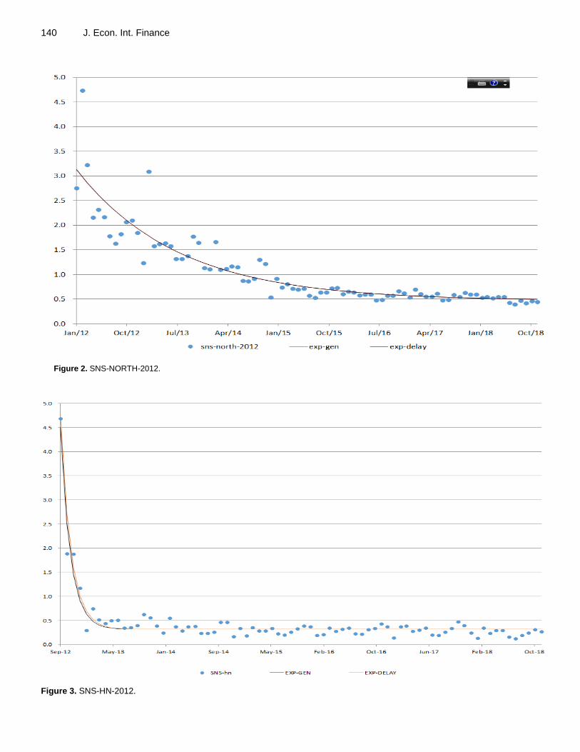
Exp-Gen model fit the data fairly well in difficult conditions, the ability to find a better model is likely minimal. Thus, the Exp-Gen model by Pegels (1969) and Towill (1990) and the exponential delay model by Evans et al. (2018) are presented in this study without any suggested modifications. The fitted lines of the two models concerning the two most divergent datasets in AIC weight (SNS-HN-2012sep and SNS-north-2012) are shown in Figures 2 and 3. The difference between the two models

2For any learning process of firms, the prior experience is supposed not to be

null.

140 J. Econ. Int. Finance

Figure 2. SNS-NORTH-2012.

Figure 3. SNS-HN-2012.

is small and difficult to distinguish as the RSS value of them is almost identical. Conclusion This study describes the mechanism of the plateau and the reason why previous studies could not locate a plateau. Two exponential models are presented as the function expressions of the law of learning by doing, both of which can provide entrepreneurs and managers with a powerful tool to predict future performance of their investment. This study also specifies that the law of learning by doing can be applied not only in individual learning but also in organizational learning. CONFLICT OF INTERESTS The author has not declared any conflict of interests. REFERENCES Akaike H (1974). A New Look at the Statistical Model Identification.‖ In

Selected Papers of Hirotugu Akaike, pp. 215-222. Springer. Anzanello MJ, Fogliatto FS (2011). Learning Curve Models and

Applications: Literature Review and Research Directions. International Journal of Industrial Ergonomics 41(5):573-83.

Arrow KJ (1962). The Economic Implications of Learning by Doing.‖ In The Review of Economic Studies, Springer 29:155. https://doi.org/10.2307/2295952.

Asher H (1956). Cost-Quantity Relationships in the Airframe Industry.‖ The Ohio State University.

Badiru AB (1992). Computational Survey of Univariate and Multivariate Learning Curve Models. IEEE Transactions on Engineering Management 39 (2):176-188.

Bates DM, Watts DG (1988). Nonlinear Regression Analysis and Its Applications. Volume 2. Wiley New York.

Benkard CL (2000). Learning and Forgetting: The Dynamics of Aircraft Production. American Economic Review 90(4):1034-1054.

Bryan WL, Harter N (1897). Studies in the Physiology and Psychology of the Telegraphic Language. Psychological Review 4(1):27.

Bryan WL, Harter N (1899). Studies on the Telegraphic Language: The Acquisition of a Hierarchy of Habits. Psychological Review 6(4):345.

Carr GW (1946). Peacetime Cost Estimating Requires New Learning Curves. Aviation 45(4):220-228.

Crossman ERFW (1959). A Theory of the Acquisition of Speed-Skill∗.‖ Ergonomics 2(2):153-166.

Dar-El EM, Ayas K, Gilad I (1995). Predicting Performance Times for Long Cycle Time Tasks. IIE Transactions 27(3):272-281.

Huhui 141 Ericsson KA, Ralf TK, Tesch-Römer C (1993). ―The Role of Deliberate

Practice in the Acquisition of Expert Performance. Psychological Review 100(3):363.

Evans NJ, Scott SD, Mewhort DJ, Heathcote A (2018). Refining the Law of Practice. Psychological Review 125(4):592.

Gray WD (2017). Plateaus and Asymptotes: Spurious and Real Limits in Human Performance. Current Directions in Psychological Science 26(1):59-67.

Gray WD, Lindstedt JK (2017). Plateaus, Dips, and Leaps: Where to Look for Inventions and Discoveries during Skilled Performance. Cognitive Science 41(7):1838-1870.

Heathcote A, Scott B, Mewhort DJK (2000). The Power Law Repealed: The Case for an Exponential Law of Practice. Psychonomic Bulletin and Review 7(2):185-207.

Hirschmann WB (1964). ―Profit from the Learning-Curve. Harvard Business Review 42(1):125-139.

Jaber MY (2006). ―Learning and Forgetting Models and Their Applications. Handbook of Industrial and Systems Engineering 30(1):30-127.

Jaber MY (2016). Learning Curves: Theory, Models, and Applications. CRC Press.

De Jong JR (1957). The Effects of Increasing Skill on Cycle Time and Its Consequences for Time Standards. Ergonomics 1(1):51-60.

Keller FS (1958). The Phantom Plateau.‖ Journal of the Experimental Analysis of Behavior 1(1):1.

Mazur JE, Reid H (1978). Learning as Accumulation: A Reexamination of the Learning Curve. Psychological Bulletin 85(6):1256.

Nembhard DA, Uzumeri MV (2000). An Individual-Based Description of Learning within an Organization. IEEE Transactions on Engineering Management 47(3):370-378.

Newell A, Rosenbloom PS (1981). ―Mechanisms of Skill Acquisition and the Law of Practice. Cognitive Skills and Their Acquisition 1(1981):1-55.

Pegels CC (1969). ―On Startup or Learning Curves: An Expanded View. AIIE Transactions 1(3):216-222.

Schwarz G (1978). ―Estimating the Dimension of a Model.‖ The Annals of Statistics 6(2):461-464.

Teplitz CJ (2014). ―Learning Curve Setbacks: You Don’t Always Move DOWN a Learning Curve. The Journal of Applied Business and Economics 16(6):32.

Thompson P (2010). ―Learning by Doing. In Handbook of the Economics of Innovation, Elsevier 1:429-476.

Thorndike EL, Woodworth RS (1901). The Influence of Improvement in One Mental Function upon the Efficiency of Other Functions.(I).‖ Psychological Review 8(3):247.

Towill DR (1990). Forecasting Learning Curves. International Journal of Forecasting 6(1):25-38.

Wright TP (1936). Factors Affecting the Cost of Airplanes. Journal of the Aeronautical Sciences 3(4):122-128.

Yelle LE (1979). The Learning Curve: Historical Review and Comprehensive Survey. Decision Sciences 10(2):302-328.