University of Pennsylvania University of Pennsylvania

ScholarlyCommons ScholarlyCommons

Statistics Papers Wharton Faculty Research

2013

Two-Sample Covariance Matrix Testing and Support Recovery Two-Sample Covariance Matrix Testing and Support Recovery

Tony Cai University of Pennsylvania

Weidong Liu

Yin Xia University of Pennsylvania

Follow this and additional works at: https://repository.upenn.edu/statistics_papers

Part of the Biostatistics Commons, and the Genetics and Genomics Commons

Recommended Citation Recommended Citation Cai, T., Liu, W., & Xia, Y. (2013). Two-Sample Covariance Matrix Testing and Support Recovery. Journal of the American Statistical Association, 108 (501), 265-277. http://dx.doi.org/10.1080/01621459.2012.758041

This paper is posted at ScholarlyCommons. https://repository.upenn.edu/statistics_papers/487 For more information, please contact repository@pobox.upenn.edu.

Two-Sample Covariance Matrix Testing and Support Recovery Two-Sample Covariance Matrix Testing and Support Recovery

Abstract Abstract This paper proposes a new test for testing the equality of two covariance matrices Σ1 and Σ2 in the high-dimensional setting and investigates its theoretical and numerical properties. The limiting null distribution of the test statistic is derived. The test is shown to enjoy certain optimality and to be especially powerful against sparse alternatives. The simulation results show that the test significantly outperforms the existing methods both in terms of size and power. Analysis of prostate cancer datasets is carried out to demonstrate the application of the testing procedures. When the null hypothesis of equal covariance matrices is rejected, it is often of significant interest to further investigate in which way they differ. Motivated by applications in genomics, we also consider two related problems, recovering the support of Σ1 − Σ2 and testing the equality of the two covariance matrices row by row. New testing procedures are introduced and their properties are studied. Applications to gene selection is also discussed.

Keywords Keywords extreme value Type 1 distribution, gene selection, hypothesis testing, sparsity

Disciplines Disciplines Biostatistics | Genetics and Genomics

This journal article is available at ScholarlyCommons: https://repository.upenn.edu/statistics_papers/487

Two-Sample Covariance Matrix Testing And

Support Recovery ∗

Tony Cai, Weidong Liu and Yin Xia

Abstract

This paper proposes a new test for testing the equality of two covariance

matrices Σ1 and Σ2 in the high-dimensional setting and investigates its the-

oretical and numerical properties. The limiting null distribution of the test

statistic is derived. The test is shown to enjoy certain optimality and to be

especially powerful against sparse alternatives. The simulation results show

that the test significantly outperforms the existing methods both in terms of

size and power. Analysis of prostate cancer datasets is carried out to demon-

strate the application of the testing procedures.

When the null hypothesis of equal covariance matrices is rejected, it is

often of significant interest to further investigate in which way they differ.

Motivated by applications in genomics, we also consider two related prob-

lems, recovering the support of Σ1 −Σ2 and testing the equality of the two

∗Tony Cai is Dorothy Silberberg Professor of Statistics, Department of Statistics, The Whar-

ton School, University of Pennsylvania, Philadelphia, PA 19104 (Email:tcai@wharton.upenn.edu).

Weidong Liu is Professor, Department of Mathematics and Institute of Natural Sciences, Shang-

hai Jiao Tong University, Shanghai, China and Postdoctoral Fellow, Department of Statis-

tics, The Wharton School, University of Pennsylvania, Philadelphia, PA 19104 (Email: liuwei-

dong99@gmail.com). Yin Xia is Ph.D student, Department of Statistics, The Wharton School,

University of Pennsylvania, Philadelphia, PA 19104 (Email: xiayin@sas.upenn.edu). The research

was supported in part by NSF FRG Grant DMS-0854973.

1

covariance matrices row by row. New testing procedures are introduced and

their properties are studied. Applications to gene selection is also discussed.

Keywords: Covariance matrix, extreme value type I distribution, gene selection,

hypothesis testing, sparsity, support recovery.

1 Introduction

Testing the equality of two covariance matrices Σ1 and Σ2 is an important prob-

lem in multivariate analysis. Many statistical procedures including the classical

Fisher’s linear discriminant analysis rely on the fundamental assumption of equal

covariance matrices. This testing problem has been well studied in the conventional

low-dimensional setting. See, for example, Sugiura and Nagao (1968), Gupta and

Giri (1973), Perlman (1980), Gupta and Tang (1984), O’Brien (1992), and Anderson

(2003). In particular, the likelihood ratio test (LRT) is commonly used and enjoys

certain optimality under regularity conditions.

Driven by a wide range of contemporary scientific applications, analysis of high

dimensional data is of significant current interest. In the high dimensional setting,

where the dimension can be much larger than the sample size, the conventional test-

ing procedures such as the LRT perform poorly or are not even well defined. Several

tests for the equality of two large covariance matrices have been proposed. For exam-

ple, Schott (2007) introduced a test based on the Frobenius norm of the difference

of the two covariance matrices. Srivastava and Yanagihara (2010) constructed a

test that relied on a measure of distance by tr(Σ21)/(tr(Σ1))

2 − tr(Σ22)/(tr(Σ2))

2.

Both of these two tests are designed for the multivariate normal populations. Chen

and Li (2011) proposed a test using a linear combination of three one-sample U -

statistics which was also motivated by an unbiased estimator of the Frobenius norm

of Σ1 −Σ2.

2

In many applications such as gene selection in genomics, the covariance matrices

of the two populations can be either equal or quite similar in the sense that they

only possibly differ in a small number of entries. In such a setting, under the

alternative the difference of the two covariance matrices Σ1 − Σ2 is sparse. The

above mentioned tests, which are all based on the Frobenius norm, are not powerful

against such sparse alternatives.

The main goal of this paper is to develop a test that is powerful against sparse

alternatives and robust with respect to the population distributions. Let X and

Y be two p variate random vectors with covariance matrices Σ1 = (σij1)p×p and

Σ2 = (σij2)p×p respectively. Let X1, . . . ,Xn1 be i.i.d. random samples from X

and let Y 1, . . . ,Y n2 be i.i.d. random samples from Y that are independent of

X1, . . . ,Xn1. We wish to test the hypotheses

H0 : Σ1 = Σ2 versus H1 : Σ1 = Σ2 (1)

based on the two samples. We are particularly interested in the high dimensional

setting where p can be much larger than n = max(n1, n2). Define the sample

covariance matrices

(σij1)p×p := Σ1 =1

n1

n1∑k=1

(Xk − X)(Xk − X)′,

(σij2)p×p := Σ2 =1

n2

n2∑k=1

(Y k − Y )(Y k − Y )′,

where X = 1n1

∑n1

k=1 Xk and Y = 1n2

∑n2

k=1 Y k.

In this paper we propose a test based on the maximum of the standardized dif-

ferences between the entries of the two sample covariance matrices and investigate

its theoretical and numerical properties. The limiting null distribution of the test

statistic is derived. It is shown that the distribution of the test statistic converges

to a type I extreme value distribution under the null H0. This fact implies that

3

the proposed test has the pre-specified significance level asymptotically. The the-

oretical analysis shows that the test enjoys certain optimality against a class of

sparse alternatives in terms of the power. In addition to the theoretical properties,

we also investigate the numerical performance of the proposed testing procedure

using both simulated and real datasets. The numerical results show that the new

test significantly outperforms the existing methods both in terms of size and power.

We also use prostate cancer datasets to demonstrate the application of our testing

procedures for gene selection.

In many applications, if the null hypothesis H0 : Σ1 = Σ2 is rejected, it is often

of significant interest to further investigate in which way the two covariance matrices

differ from each other. Motivated by applications to gene selection, in this paper we

also consider two related problems, recovering the support of Σ1 −Σ2 and testing

the equality of the two covariance matrices row by row. Support recovery can also be

viewed as simultaneous testing of the equality of individual entries between the two

covariance matrices. We introduce a procedure for support recovery based on the

thresholding of the standardized differences between the entries of the two covariance

matrices. It is shown that under certain conditions, the procedure recovers the true

support of Σ1 − Σ2 exactly with probability tending to 1. The procedure is also

shown to be minimax rate optimal.

The problem of testing the equality of two covariance matrices row by row is

motivated by applications in genomics. A commonly used approach in microarray

analysis is to select “interesting” genes by applying multiple testing procedures

on the two-sample t-statistics. This approach has been successful in finding genes

with significant changes in the mean expression levels between diseased and non-

diseased populations. It has been noted recently that these mean-based methods

lack the ability to discover genes that change their relationships with other genes

and new methods that are based on the change in the gene’s dependence structure

4

are thus needed to identify these genes. See, for example, Ho, et al. (2008), Hu,

et al. (2009) and Hu, et al. (2010). In this paper, we propose a procedure which

simultaneously tests the p null hypotheses that the corresponding rows of the two

covariance matrices are equal to each other. Asymptotic null distribution of the

test statistics is derived and properties of the test is studied. It is shown that the

procedure controls the family-wise error rate at a pre-specified level. Applications

to gene selection is also considered.

The rest of this paper is organized as follows. Section 2 introduces the procedure

for testing the equality of two covariance matrices. Theoretical properties of the

test are investigated in Section 3. After Section 3.1 in which basic definitions and

assumptions are given, Section 3.2 develops the asymptotic null distribution of the

test statistic and presents the optimality results in terms of the power of the test

against sparse alternatives. Section 4 considers support recovery of Σ1 − Σ2 and

testing the two covariance matrices row by row. Applications to gene selection is

also discussed. Section 5 investigates the numerical performance of the proposed

tests by simulations and by applications to the analysis of prostate cancer datasets.

Section 6 discusses our results and other related work. The proofs of the main

results are given in Section 7.

2 The testing procedure

The null hypothesis H0 : Σ1 = Σ2 is equivalent to H0 : max1≤i≤j≤p |σij1 − σij2| = 0.

A natural approach to testing this hypothesis is to compare the sample covariances

σij1 and σij2 and to base the test on the maximum differences. It is important to

note that the sample covariances σij1’s and σij2’s are in general heteroscedastic and

can possibly have a wide range of variability. It is thus necessary to first standardize

σij1 − σij2 before making a comparison among different entries.

5

To be more specific, define the variances θij1 = Var((Xi − µ1i)(Xj − µ1j))

and θij2 = Var((Yi − µ2i)(Yj − µ2j)). Given the two samples X1, . . . ,Xn1 and

Y 1, . . . ,Y n2, θij1 and θij2 can be respectively estimated by

θij1 =1

n1

n1∑k=1

[(Xki − Xi)(Xkj − Xj)− σij1

]2, Xi =

1

n1

n1∑k=1

Xki,

and

θij2 =1

n2

n2∑k=1

[(Yki − Yi)(Ykj − Yj)− σij2

]2, Yi =

1

n2

n2∑k=1

Yki.

Such an estimator of the variance have been used in Cai and Liu (2011) in the

context of adaptive estimation of a sparse covariance matrix. Given θij1 and θij2,

the variance of σij1 − σij2 can then be estimated by θij1/n1 + θij2/n2.

Define the standardized statistics

Wij =:σij1 − σij2√

θij1/n1 + θij2/n2

and Mij =: W 2ij, , 1 ≤ i ≤ j ≤ p. (2)

We consider the following test statistic for testing the hypothesis H0 : Σ1 = Σ2,

Mn =: max1≤i≤j≤p

Mij = max1≤i≤j≤p

(σij1 − σij2)2

θij1/n1 + θij2/n2

. (3)

The asymptotic behavior of the test statistic Mn will be studied in detail in

Section 3. Intuitively, Wij are approximately standard normal variables under the

null H0 and the Mij are only “weakly dependent” under suitable conditions. The

test statistic Mn is the maximum of p2 such variables and so the value of Mn is

close to 2 log p2 under H0, based on the extreme values of normal random variables.

More precisely, we shall show in Section 3 that, under certain regularity conditions,

Mn − 4 log p + log log p converges to a type I extreme value distribution under the

null hypothesis H0. Based on this result, for a given significance level 0 < α < 1,

we define the test Φα by

Φα = I(Mn ≥ qα + 4 log p− log log p) (4)

6

where qα is the 1 − α quantile of the type I extreme value distribution with the

cumulative distribution function exp(− 1√8π

exp(−x2)), i.e.,

qα = − log(8π)− 2 log log(1− α)−1. (5)

The hypothesis H0 : Σ1 = Σ2 is rejected whenever Φα = 1.

The test Φα is particularly well suited for testing against sparse alternatives. It

is consistent if one of the entries of Σ1−Σ2 has a magnitude no less than C√

log p/n

for some constant C > 0 and no other special structure of Σ1 −Σ2 is required. It

will be shown that the test Φα is an asymptotically α-level test and enjoys certain

optimality against sparse alternatives.

In addition, the standardized statistics Mij are useful for identifying the support

of Σ1 − Σ2. That is, they can be used to estimate the positions at which the two

covariance matrices differ from each other. This is of particular interest in many

applications including gene selection. We shall show in Section 4.1 that under certain

conditions, the support of Σ1 −Σ2 can be correctly recovered by thresholding the

Mij.

3 Theoretical analysis of size and power

We now turn to an analysis of the properties of the test Φα including the asymptotic

size and power. The asymptotic size of the test is obtained by deriving the limiting

distribution of the test statistic Mn under the null. We are particularly interested

in the power of the test Φα under the sparse alternatives where Σ1 −Σ2 are sparse

in the sense that Σ1 −Σ2 only contains a small number of nonzero entries.

7

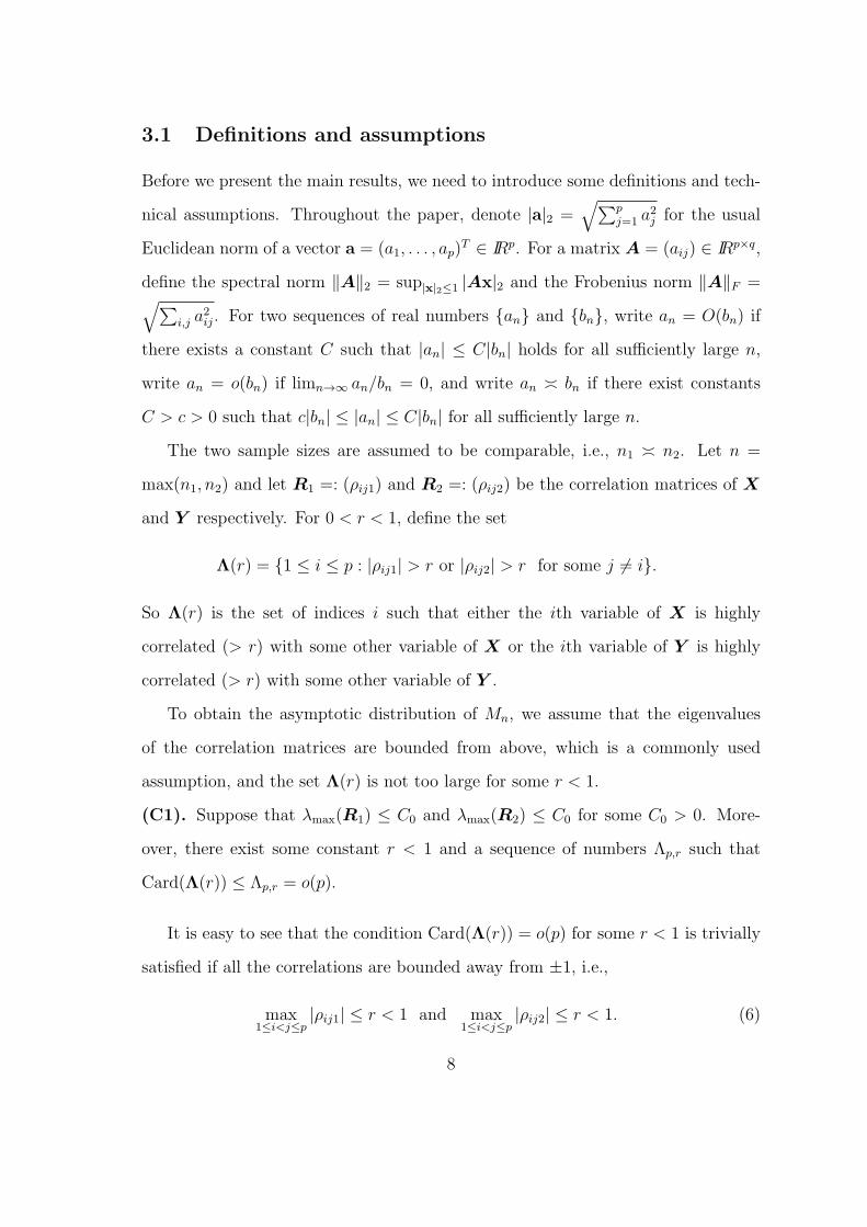
3.1 Definitions and assumptions

Before we present the main results, we need to introduce some definitions and tech-

nical assumptions. Throughout the paper, denote |a|2 =√∑p

j=1 a2j for the usual

Euclidean norm of a vector a = (a1, . . . , ap)T ∈ IRp. For a matrix A = (aij) ∈ IRp×q,

define the spectral norm ∥A∥2 = sup|x|2≤1 |Ax|2 and the Frobenius norm ∥A∥F =√∑i,j a

2ij. For two sequences of real numbers an and bn, write an = O(bn) if

there exists a constant C such that |an| ≤ C|bn| holds for all sufficiently large n,

write an = o(bn) if limn→∞ an/bn = 0, and write an ≍ bn if there exist constants

C > c > 0 such that c|bn| ≤ |an| ≤ C|bn| for all sufficiently large n.

The two sample sizes are assumed to be comparable, i.e., n1 ≍ n2. Let n =

max(n1, n2) and let R1 =: (ρij1) and R2 =: (ρij2) be the correlation matrices of X

and Y respectively. For 0 < r < 1, define the set

Λ(r) = 1 ≤ i ≤ p : |ρij1| > r or |ρij2| > r for some j = i.

So Λ(r) is the set of indices i such that either the ith variable of X is highly

correlated (> r) with some other variable of X or the ith variable of Y is highly

correlated (> r) with some other variable of Y .

To obtain the asymptotic distribution of Mn, we assume that the eigenvalues

of the correlation matrices are bounded from above, which is a commonly used

assumption, and the set Λ(r) is not too large for some r < 1.

(C1). Suppose that λmax(R1) ≤ C0 and λmax(R2) ≤ C0 for some C0 > 0. More-

over, there exist some constant r < 1 and a sequence of numbers Λp,r such that

Card(Λ(r)) ≤ Λp,r = o(p).

It is easy to see that the condition Card(Λ(r)) = o(p) for some r < 1 is trivially

satisfied if all the correlations are bounded away from ±1, i.e.,

max1≤i<j≤p

|ρij1| ≤ r < 1 and max1≤i<j≤p

|ρij2| ≤ r < 1. (6)

8

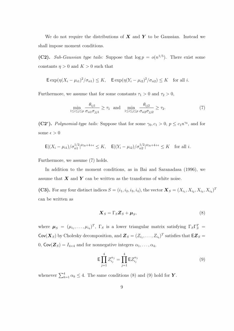
We do not require the distributions of X and Y to be Gaussian. Instead we

shall impose moment conditions.

(C2). Sub-Gaussian type tails: Suppose that log p = o(n1/5). There exist some

constants η > 0 and K > 0 such that

E exp(η(Xi − µi1)2/σii1) ≤ K, E exp(η(Yi − µi2)

2/σii2) ≤ K for all i.

Furthermore, we assume that for some constants τ1 > 0 and τ2 > 0,

min1≤i≤j≤p

θij1σii1σjj1

≥ τ1 and min1≤i≤j≤p

θij2σii2σjj2

≥ τ2. (7)

(C2∗). Polynomial-type tails: Suppose that for some γ0, c1 > 0, p ≤ c1nγ0 , and for

some ϵ > 0

E|(Xi − µi1)/σ1/2ii1 |4γ0+4+ϵ ≤ K, E|(Yi − µi2)/σ

1/2ii2 |4γ0+4+ϵ ≤ K for all i.

Furthermore, we assume (7) holds.

In addition to the moment conditions, as in Bai and Saranadasa (1996), we

assume that X and Y can be written as the transforms of white noise.

(C3). For any four distinct indices S = (i1, i2, i3, i4), the vectorXS = (Xi1 , Xi2 , Xi3 , Xi4)T

can be written as

XS = ΓSZS + µS, (8)

where µS = (µi1 , . . . , µi4)T , ΓS is a lower triangular matrix satisfying ΓSΓ

TS =

Cov(XS) by Cholesky decomposition, and ZS = (Zi1 , . . . , Zi4)T satisfies that EZS =

0, Cov(ZS) = I4×4 and for nonnegative integers α1, . . . , α4,

E4∏

j=1

Zαj

ij=

4∏j=1

EZαj

ij(9)

whenever∑4

k=1 αk ≤ 4. The same conditions (8) and (9) hold for Y .

9

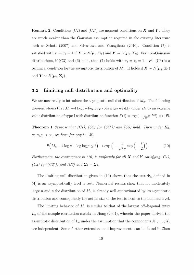
Remark 2. Conditions (C2) and (C2∗) are moment conditions on X and Y . They

are much weaker than the Gaussian assumption required in the existing literature

such as Schott (2007) and Srivastava and Yanagihara (2010). Condition (7) is

satisfied with τ1 = τ2 = 1 if X ∼ N(µ1,Σ1) and Y ∼ N(µ2,Σ2). For non-Gaussian

distributions, if (C3) and (6) hold, then (7) holds with τ1 = τ2 = 1 − r2. (C3) is a

technical condition for the asymptotic distribution ofMn. It holds ifX ∼ N(µ1,Σ1)

and Y ∼ N(µ2,Σ2).

3.2 Limiting null distribution and optimality

We are now ready to introduce the asymptotic null distribution ofMn. The following

theorem shows that Mn−4 log p+log log p converges weakly under H0 to an extreme

value distribution of type I with distribution function F (t) = exp(− 1√8πe−t/2), t ∈ IR.

Theorem 1 Suppose that (C1), (C2) (or (C2∗)) and (C3) hold. Then under H0,

as n, p → ∞, we have for any t ∈ IR,

P(Mn − 4 log p+ log log p ≤ t

)→ exp

(− 1√

8πexp

(− t

2

)). (10)

Furthermore, the convergence in (10) is uniformly for all X and Y satisfying (C1),

(C2) (or (C2∗)) and (C3) and Σ1 = Σ2.

The limiting null distribution given in (10) shows that the test Φα defined in

(4) is an asymptotically level α test. Numerical results show that for moderately

large n and p the distribution of Mn is already well approximated by its asymptotic

distribution and consequently the actual size of the test is close to the nominal level.

The limiting behavior of Mn is similar to that of the largest off-diagonal entry

Ln of the sample correlation matrix in Jiang (2004), wherein the paper derived the

asymptotic distribution of Ln under the assumption that the componentsX1, . . . , Xp

are independent. Some further extensions and improvements can be found in Zhou

10

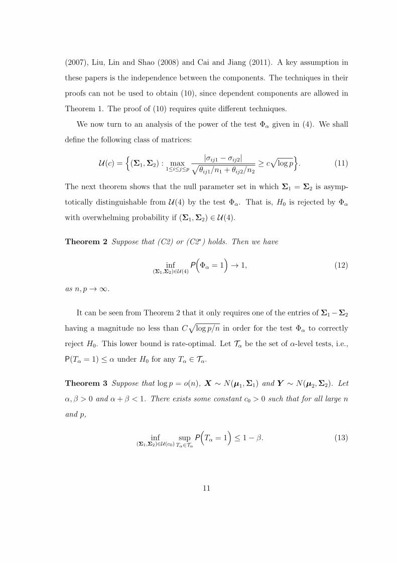
(2007), Liu, Lin and Shao (2008) and Cai and Jiang (2011). A key assumption in

these papers is the independence between the components. The techniques in their

proofs can not be used to obtain (10), since dependent components are allowed in

Theorem 1. The proof of (10) requires quite different techniques.

We now turn to an analysis of the power of the test Φα given in (4). We shall

define the following class of matrices:

U(c) =(Σ1,Σ2) : max

1≤i≤j≤p

|σij1 − σij2|√θij1/n1 + θij2/n2

≥ c√log p

. (11)

The next theorem shows that the null parameter set in which Σ1 = Σ2 is asymp-

totically distinguishable from U(4) by the test Φα. That is, H0 is rejected by Φα

with overwhelming probability if (Σ1,Σ2) ∈ U(4).

Theorem 2 Suppose that (C2) or (C2∗) holds. Then we have

inf(Σ1,Σ2)∈U(4)

P(Φα = 1

)→ 1, (12)

as n, p → ∞.

It can be seen from Theorem 2 that it only requires one of the entries of Σ1−Σ2

having a magnitude no less than C√

log p/n in order for the test Φα to correctly

reject H0. This lower bound is rate-optimal. Let Tα be the set of α-level tests, i.e.,

P(Tα = 1) ≤ α under H0 for any Tα ∈ Tα.

Theorem 3 Suppose that log p = o(n), X ∼ N(µ1,Σ1) and Y ∼ N(µ2,Σ2). Let

α, β > 0 and α+ β < 1. There exists some constant c0 > 0 such that for all large n

and p,

inf(Σ1,Σ2)∈U(c0)

supTα∈Tα

P(Tα = 1

)≤ 1− β. (13)

11

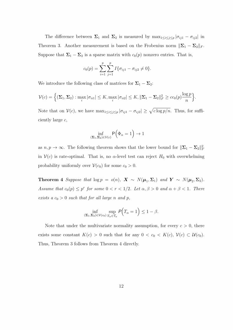
The difference between Σ1 and Σ2 is measured by max1≤i≤j≤p |σij1 − σij2| in

Theorem 3. Another measurement is based on the Frobenius norm ∥Σ1 − Σ2∥F .

Suppose that Σ1 −Σ2 is a sparse matrix with c0(p) nonzero entries. That is,

c0(p) =

p∑i=1

p∑j=1

Iσij1 − σij2 = 0.

We introduce the following class of matrices for Σ1 −Σ2:

V(c) =(Σ1,Σ2) : max

i|σii1| ≤ K,max

i|σii2| ≤ K, ∥Σ1 −Σ2∥2F ≥ cc0(p)

log p

n

.

Note that on V(c), we have max1≤i≤j≤p |σij1 − σij2| ≥√

c log p/n. Thus, for suffi-

ciently large c,

inf(Σ1,Σ2)∈V(c)

P(Φα = 1

)→ 1

as n, p → ∞. The following theorem shows that the lower bound for ∥Σ1 − Σ2∥2Fin V(c) is rate-optimal. That is, no α-level test can reject H0 with overwhelming

probability uniformly over V(c0) for some c0 > 0.

Theorem 4 Suppose that log p = o(n), X ∼ N(µ1,Σ1) and Y ∼ N(µ2,Σ2).

Assume that c0(p) ≤ pr for some 0 < r < 1/2. Let α, β > 0 and α + β < 1. There

exists a c0 > 0 such that for all large n and p,

inf(Σ1,Σ2)∈V(c0)

supTα∈Tα

P(Tα = 1

)≤ 1− β.

Note that under the multivariate normality assumption, for every c > 0, there

exists some constant K(c) > 0 such that for any 0 < c0 < K(c), V(c) ⊂ U(c0).

Thus, Theorem 3 follows from Theorem 4 directly.

12

4 Support recovery of Σ1 −Σ2 and application to

gene selection

We have focused on testing the equality of two covariance matrices Σ1 and Σ2 in

Sections 2 and 3. As mentioned in the introduction, if the null hypothesis H0 :

Σ1 = Σ2 is rejected, further exploring in which ways they differ is also of significant

interest in practice. Motivated by applications in gene selection, we consider in this

section two related problems, one is recovering the support of Σ1 −Σ2 and another

is identifying the rows on which the two covariance matrices differ from each other.

4.1 Support recovery of Σ1 −Σ2

The goal of support recovery is to find the positions at which the two covariance

matrices differ from each other. The problem can also be viewed as simultaneous

testing of equality of individual entries between the two covariance matrices. Denote

the support of Σ1 −Σ2 by

Ψ = Ψ(Σ1,Σ2) = (i, j) : σij1 = σij2. (14)

In certain applications, the variances along the diagonal play a more important

role than the covariances. For example, in a differential variability analysis of gene

expression Ho, et al (2008) proposed to select genes based on the differences in the

variances. In this section we shall treat the variances along the diagonal differently

from the off-diagonal covariances for support recovery. Since there are p diagonal

elements, Mii along the diagonal are thresholded at 2 log p based on the extreme

values of normal variables. The off-diagonal entries Mij with i = j are thresholded

at a different level. More specifically, set

Ψ(τ) = (i, i) : Mii ≥ 2 log p ∪ (i, j) : Mij ≥ τ log p, i = j, (15)

13

where Mij are defined in (2) and τ is the threshold constant for the off-diagonal

entries.

The following theorem shows that with τ = 4 the estimator Ψ(4) recovers the

support Ψ exactly with probability tending to 1 when the magnitudes of nonzero

entries are above certain thresholds. Define

W0(c) =(Σ1,Σ2) : min

(i,j)∈Ψ

|σij1 − σij2|√θij1/n1 + θij2/n2

≥ c√

log p.

We have the following result.

Theorem 5 Suppose that (C2) or (C2∗) holds. Then

inf(Σ1,Σ2)∈W0(4)

P(Ψ(4) = Ψ

)→ 1

as n, p → ∞.

The choice of the threshold constant τ = 4 is optimal for the exact recovery of

the support Ψ. Consider the class of s0(p)-sparse matrices,

S0 =A = (aij)p×p : max

i

p∑j=1

Iaij = 0 ≤ s0(p).

Theorem 6 Suppose that (C1), (C2) (or (C2∗)) and (C3) hold. Let 0 < τ < 4. If

s0(p) = O(p1−τ1) with some τ/4 < τ1 < 1, then as n, p → ∞,

supΣ1−Σ2∈S0

P(Ψ(τ) = Ψ

)→ 0.

In other words, for any threshold constant τ < 4, the probability of recovering the

support exactly tends to 0 for all Σ1 −Σ2 ∈ S0. This is mainly due to the fact that

the threshold level τ log p is too small to ensure that the zero entries of Σ1−Σ2 are

estimated by zero.

In addition, the minimum separation of the magnitudes of the nonzero entries

must be at least of order√log p/n to enable the exact recovery of the support.

14

Consider, for example, s0(p) = 1 in Theorem 4. Then Theorem 4 indicates that

no test can distinguish H0 and H1 uniformly on the space V(c0) with probability

tending to one. It is easy to see that V(c0) ⊆ W0(c1) for some c1 > 0. Hence, there

is no estimate that can recover the support Ψ exactly uniformly on the space W0(c1)

with probability tending to one.

We have so far focused on the exact recovery of the support of Σ1 − Σ2 with

probability tending to 1. It is sometimes desirable to recover the support under

a less stringent criterion such as the family-wise error rate (FWER), defined by

FWER = P(V ≥ 1), where V is the number of false discoveries. The goal of using

the threshold level 4 log p is to ensure FWER → 0. To control the FWER at a

pre-specified level α for some 0 < α < 1, a different threshold level is needed. For

this purpose, we shall set the threshold level at 4 log p − log log p + qα where qα is

given in (5). Define

Ψ⋆ = (i, i) : Mii ≥ 2 log p ∪ (i, j) : Mij ≥ 4 log p− log log p+ qα, i = j.

We have the following result.

Proposition 1 Suppose that (C1), (C2) (or (C2∗)) and (C3) hold. Under Σ1 −

Σ2 ∈ S0 ∩W0(4) with s0(p) = o(p), we have as n, p → ∞,

P(Ψ⋆ = Ψ

)→ α.

4.2 Testing rows of two covariance matrices

As discussed in the introduction, the standard methods for gene selection are based

on the comparisons of the means and thus lack the ability to select genes that change

their relationships with other genes. It is of significant practical interest to develop

methods for gene selection which capture the changes in the gene’s dependence

structure.

15

Several methods have been proposed in the literature. It was noted in Ho, et al.

(2008) that the changes of variances are biologically interesting and are associated

with changes in coexpression patterns in different biological states. Ho, et al. (2008)

proposed to test H0i : σii1 = σii2 and select the i-th gene if H0i is rejected, and

Hu, et al. (2009) and Hu, et al. (2010) introduced methods which are based on

simultaneous testing of the equality of the joint distributions of each row between

two sample correlation matrices/covariance distance matrices.

The covariance provides a natural measure of the association between two genes

and it can also reflect the changes of variances. Motivated by these applications, in

this section we consider testing the equality of two covariance matrices row by row.

Let σi·1 and σi·2 be the i-th row of Σ1 and Σ2 respectively. We consider testing

simultaneously the hypotheses

H0i : σi·1 = σi·2, 1 ≤ i ≤ p.

We shall use the family-wise error rate (FWER) to measure the type I errors for

the p tests. The support estimate Ψ(4) defined in (15) can be used to test the

hypotheses H0i by rejecting H0i if the i-th row of Ψ(4) is nonzero. Suppose that

(C1) and (C2) (or (C2∗)) hold. Then it can be shown easily that for this test, the

FWER → 0.

A different test is needed to simultaneously test the hypotheses H0i, 1 ≤ i ≤ p,

at a pre-specified FWER level α for some 0 < α < 1. Define

Mi· = max1≤j≤p,j =i

(σij1 − σij2)2

θij1/n1 + θij2/n2

.

The null distribution of Mi· can be derived similarly under the same conditions as

in Theorem 1.

Proposition 2 Suppose the null hypothesis H0i holds. Then under the conditions

16

in Theorem 1,

P(Mi· − 2 log p+ log log p ≤ x

)→ exp

(− 1√

πexp

(− x

2

)). (16)

Based on the limiting null distribution of Mi· given in (16), we introduce the follow-

ing test for testing a single hypothesis H0i,

Φi,α = I(Mi· ≥ αp or Mii ≥ 2 log p) (17)

with αp = 4 log p− log log p+ qα, where qα is given in (5).

H0i is rejected and the i-th gene is selected if Φi,α = 1. It can be shown that the

tests Φi,α, 1 ≤ i ≤ p together controls the overall FWER at level α asymptotically.

Proposition 3 Let F = i : σi·1 = σi·2, 1 ≤ i ≤ p and suppose Card(F ) = o(p).

Then under the conditions in Theorem 1,

FWER = P(maxi∈F c

Φi,α = 1)→ α.

5 Numerical results

In this section, we turn to the numerical performance of the proposed methods. The

goal is to first investigate the numerical performance of the test Φα and support

recovery through simulation studies and then illustrate our methods by applying

them to the analysis of a prostate cancer dataset. The test Φα is compared with

four other tests, the likelihood ratio test (LRT), the tests given in Schott (2007) and

Chen and Li (2011) which are both based on an unbiased estimator of ∥Σ1 −Σ2∥2F ,

the test proposed in Srivastava and Yanagihara (2009) which is based on a measure

of distance by tr(Σ21)/(tr(Σ1))

2 − tr(Σ22)/(tr(Σ2))

2.

We first introduce the matrix models used in the simulations. Let D = (dij) be

a diagonal matrix with diagonal elements dii = Unif(0.5, 2.5) for i = 1, ..., p. Denote

17

by λmin(A) the minimum eigenvalue of a symmetric matrix A. The following four

models under the null, Σ1 = Σ2 = Σ(i), i = 1, 2, 3 and 4, are used to study the size

of the tests.

• Model 1: Σ∗(1) = (σ∗(1)ij ) where σ

∗(1)ii = 1, σ

∗(1)ij = 0.5 for 5(k − 1) + 1 ≤ i =

j ≤ 5k, where k = 1, ..., [p/5] and σ∗(1)ij = 0 otherwise. Σ(1) = D1/2Σ∗(1)D1/2.

• Model 2: Σ∗(2) = (σ∗(2)ij ) where ω

∗(2)ij = 0.5|i−j| for 1 ≤ i, j ≤ p. Σ(2) =

D1/2Σ∗(2)D1/2.

• Model 3: Σ∗(3) = (σ(3)ij ) where σ

∗(3)ii = 1, σ

∗(3)ij = 0.5 ∗ Bernoulli(1, 0.05) for

i < j and σ∗(3)ji = σ

∗(3)ij . Σ(3) = D1/2(Σ∗(3) + δI)/(1 + δ)D1/2 with δ =

|λmin(Σ∗(3))|+ 0.05.

• Model 4: Σ(4) = O∆O, where O = diag(ω1, ..., ωp) and ω1, ..., ωpiid∼ Unif(1, 5)

and ∆ = (aij) and aij = (−1)i+j0.4|i−j|1/10 . This model was used in Srivastava

and Yanagihara (2009).

To evaluate the power of the tests, let U = (ukl) be a matrix with 8 random

nonzero entries. The locations of 4 nonzero entries are selected randomly from the

upper triangle of U , each with a magnitude generated from Unif(0, 4)∗max1≤j≤p σjj.

The other 4 nonzero entries in the lower triangle are determined by symmetry. We

use the following four pairs of covariance matrices (Σ(i)1 ,Σ

(i)2 ), i = 1, 2, 3 and 4, to

compare the power of the tests, where Σ(i)1 = Σ(i) + δI and Σ

(i)2 = Σ(i) +U + δI,

with δ = |minλmin(Σ(i) +U), λmin(Σ

(i))|+ 0.05.

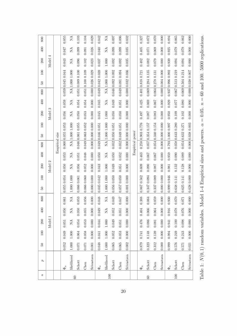
The sample sizes are taken to be n1 = n2 = n with n = 60 and 100, while the

dimension p varies over the values 50, 100, 200, 400 and 800. For each model, data

are generated from multivariate normal distributions with mean zero and covariance

matrices Σ1 and Σ2. The nominal significant level for all the tests is set at α = 0.05.

18

The actual sizes and powers for the four models, reported in Table 1, are estimated

from 5000 replications.

It can be seen from Table 1 that the estimated sizes of our test Φα are close to the

nominal level 0.05 in all the cases. This reflects the fact that the null distribution of

the test statisticMn is well approximated by its asymptotic distribution. For Models

1-3, the estimated sizes of the tests in Schott (2007) and Chen and Li (2011) are

also close to 0.05. But both tests suffer from the size distortion for Model 4, the

actual sizes are around 0.10 for both tests. The likelihood ratio test has serious

size distortion (all is equal to 1). Srivastava and Yanagihara (2010)’s test has actual

sizes close to the nominal significance level only in the fourth model, with the actual

sizes all close to 0 in the first three models.

The power results in Table 1 show that the proposed test has much higher power

than the other tests in all settings. The number of nonzero off-diagonal entries of

Σ1 − Σ2 does not change when p grows, so the estimated powers of all tests tend

to decrease when the dimension p increases. It can be seen in Table 1 that the

powers of Schott (2007) and Chen and Li (2011)’s tests decrease extremely fast as

p grows. Srivastava and Yanagihara (2010)’s test has trivial powers no matter how

large p is. However, the power of the proposed test Φα remains high even when

p = 800, especially in the case of n = 100. Overall, for the sparse models, the new

test significantly outperforms all the other three tests.

We also carried out simulations for non-Gaussian distributions including Gamma

distribution, t distribution and normal distribution contaminated with exponential

distribution. Similar phenomena as those in the Gaussian case are observed. For

reasons of space, these simulation results are given in the supplementary material,

Cai, Liu and Xia (2011).

19

np

5010

020

040

080

050

100

200

400

800

50

100

200

400

800

50100

200

400

800

Model

1Model

2Model

3Model

4

Empiricalsize

60

Φα

0.052

0.049

0.051

0.056

0.061

0.0550.054

0.050

0.053

0.060

0.055

0.053

0.056

0.059

0.0590.04

50.044

0.043

0.047

0.055

likelihood

1.000

1.000

NA

NA

NA

1.0001.000

NA

NA

NA

1.000

1.000

NA

NA

NA

1.00

01.000

NA

NA

NA

Schott

0.071

0.064

0.054

0.050

0.053

0.0660.061

0.056

0.051

0.046

0.061

0.055

0.050

0.054

0.0510.08

90.100

0.096

0.099

0.103

Chen

0.071

0.058

0.053

0.055

0.056

0.0660.060

0.052

0.048

0.049

0.063

0.052

0.053

0.054

0.0510.10

00.109

0.102

0.091

0.104

Srivastava

0.001

0.000

0.000

0.000

0.000

0.0000.000

0.000

0.000

0.000

0.000

0.000

0.000

0.000

0.0000.02

60.029

0.023

0.026

0.029

100

Φα

0.048

0.041

0.044

0.049

0.048

0.0450.042

0.043

0.050

0.049

0.046

0.051

0.045

0.045

0.0490.04

20.039

0.037

0.040

0.042

likelihood

1.000

1.000

1.000

NA

NA

1.0001.000

1.000

NA

NA

1.000

1.000

1.000

NA

NA

1.00

01.000

1.000

NA

NA

Schott

0.065

0.052

0.049

0.052

0.049

0.0560.050

0.049

0.050

0.052

0.050

0.051

0.050

0.049

0.0460.09

20.092

0.092

0.099

0.097

Chen

0.065

0.053

0.051

0.051

0.047

0.0570.050

0.051

0.052

0.052

0.049

0.051

0.050

0.051

0.0490.09

10.094

0.092

0.099

0.096

Srivastava

0.002

0.000

0.000

0.000

0.000

0.0010.000

0.000

0.000

0.000

0.000

0.000

0.000

0.000

0.0000.03

20.036

0.035

0.035

0.032

Empirical

pow

er

60

Φα

0.879

0.741

0.476

0.404

0.388

0.8670.562

0.609

0.463

0.258

0.903

0.776

0.497

0.425

0.4010.81

80.721

0.482

0.405

0.327

Schott

0.323

0.148

0.086

0.066

0.064

0.3470.094

0.090

0.067

0.057

0.354

0.157

0.087

0.069

0.0690.28

40.135

0.082

0.071

0.072

Chen

0.312

0.139

0.081

0.064

0.059

0.3370.089

0.087

0.067

0.054

0.340

0.154

0.083

0.067

0.0640.27

80.131

0.079

0.069

0.070

Srivastava

0.000

0.000

0.000

0.000

0.000

0.0000.000

0.000

0.000

0.000

0.000

0.000

0.000

0.000

0.0000.00

40.000

0.000

0.000

0.000

100

Φα

0.999

0.994

0.941

0.916

0.930

0.9990.946

0.981

0.959

0.793

1.000

0.997

0.950

0.929

0.9370.99

60.992

0.939

0.925

0.894

Schott

0.576

0.249

0.100

0.078

0.070

0.6380.141

0.132

0.090

0.058

0.643

0.280

0.109

0.077

0.0670.51

30.219

0.094

0.079

0.065

Chen

0.571

0.243

0.098

0.076

0.071

0.6250.141

0.128

0.089

0.054

0.632

0.271

0.102

0.080

0.0690.50

40.214

0.094

0.079

0.062

Srivastava

0.021

0.000

0.000

0.000

0.000

0.0280.000

0.000

0.000

0.000

0.038

0.003

0.000

0.000

0.0000.03

80.007

0.000

0.000

0.000

Tab

le1:

N(0,1)random

variab

les.

Model

1-4Empirical

sizesan

dpow

ers.

α=

0.05.n=

60an

d100.

5000

replication

s.

20

5.1 Support recovery

We now consider the simulation results on recovering the support of Σ1 − Σ2 in

the first three models with D = I and the fourth model with O = I under the

normal distribution. For i = 1, 2, 3 and 4, let U (i) be a matrix with 50 random

nonzero entries, each with a magnitude of 2 and let Σ(i)1 = (Σ(i) + δI)/(1 + δ) and

Σ(i)2 = (Σ(i)+U (i)+ δI)/(1+ δ) with δ = |min(λmin(Σ

(i)+U (i)), λmin(Σ(i)))|+0.05.

After normalization, the nonzero elements of Σ(i)2 − Σ

(i)1 have magnitude between

0.74 and 0.86 for i = 1, 2, 3 and 4 in our generated models.

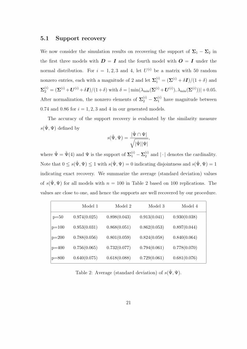
The accuracy of the support recovery is evaluated by the similarity measure

s(Ψ,Ψ) defined by

s(Ψ,Ψ) =|Ψ ∩Ψ|√|Ψ||Ψ|

,

where Ψ = Ψ(4) and Ψ is the support of Σ(i)1 −Σ

(i)2 and | · | denotes the cardinality.

Note that 0 ≤ s(Ψ,Ψ) ≤ 1 with s(Ψ,Ψ) = 0 indicating disjointness and s(Ψ,Ψ) = 1

indicating exact recovery. We summarize the average (standard deviation) values

of s(Ψ,Ψ) for all models with n = 100 in Table 2 based on 100 replications. The

values are close to one, and hence the supports are well recovered by our procedure.

Model 1 Model 2 Model 3 Model 4

p=50 0.974(0.025) 0.898(0.043) 0.913(0.041) 0.930(0.038)

p=100 0.953(0.031) 0.868(0.051) 0.862(0.053) 0.897(0.044)

p=200 0.788(0.056) 0.801(0.059) 0.824(0.058) 0.840(0.064)

p=400 0.756(0.065) 0.732(0.077) 0.794(0.061) 0.778(0.070)

p=800 0.640(0.075) 0.618(0.088) 0.729(0.061) 0.681(0.076)

Table 2: Average (standard deviation) of s(Ψ,Ψ).

21

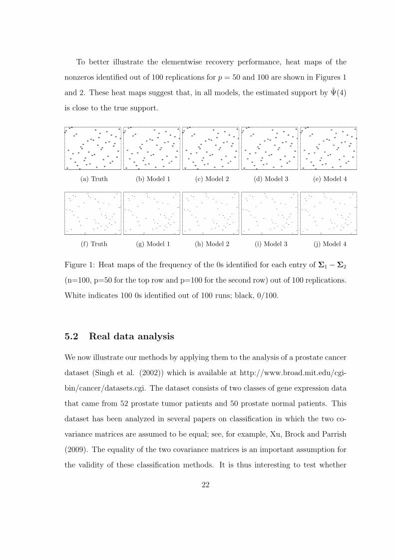
To better illustrate the elementwise recovery performance, heat maps of the

nonzeros identified out of 100 replications for p = 50 and 100 are shown in Figures 1

and 2. These heat maps suggest that, in all models, the estimated support by Ψ(4)

is close to the true support.

5

10

15

20

25

30

35

40

45

50

(a) Truth

5

10

15

20

25

30

35

40

45

50

(b) Model 1

5

10

15

20

25

30

35

40

45

50

(c) Model 2

5

10

15

20

25

30

35

40

45

50

(d) Model 3

5

10

15

20

25

30

35

40

45

50

(e) Model 4

10

20

30

40

50

60

70

80

90

100

(f) Truth

10

20

30

40

50

60

70

80

90

100

(g) Model 1

10

20

30

40

50

60

70

80

90

100

(h) Model 2

10

20

30

40

50

60

70

80

90

100

(i) Model 3

10

20

30

40

50

60

70

80

90

100

(j) Model 4

Figure 1: Heat maps of the frequency of the 0s identified for each entry of Σ1 −Σ2

(n=100, p=50 for the top row and p=100 for the second row) out of 100 replications.

White indicates 100 0s identified out of 100 runs; black, 0/100.

5.2 Real data analysis

We now illustrate our methods by applying them to the analysis of a prostate cancer

dataset (Singh et al. (2002)) which is available at http://www.broad.mit.edu/cgi-

bin/cancer/datasets.cgi. The dataset consists of two classes of gene expression data

that came from 52 prostate tumor patients and 50 prostate normal patients. This

dataset has been analyzed in several papers on classification in which the two co-

variance matrices are assumed to be equal; see, for example, Xu, Brock and Parrish

(2009). The equality of the two covariance matrices is an important assumption for

the validity of these classification methods. It is thus interesting to test whether

22

such an assumption is valid.

There are a total of 12600 genes. To control the computational costs, only the

5000 genes with the largest absolute values of the t-statistics are used. Let Σ1 and

Σ2 be respectively the covariance matrices of these 5000 genes in tumor and normal

samples. We apply the test Φα defined in (4) to test the hypotheses H0 : Σ1 = Σ2

versus H1 : Σ1 = Σ2. Based on the asymptotic distribution of the test statistic Mn,

the p-value is calculated to be 0.0058 and the null hypothesis H0 : Σ1 = Σ2 is thus

rejected at commonly used significant levels such as α = 0.05 or α = 0.01. Based

on this test result, it is therefore not reasonable to assume Σ1 = Σ2 in applying a

classifier to this dataset.

We then apply three methods to select genes with changes in variances/covariances

between the two classes. The first is the differential variability analysis (Ho, et al.,

2008) which chooses the genes with different variances between two classes. In

our procedure the i-th gene is selected if Mii ≥ 2 log p. As a result, 21 genes are

selected. The second and third methods are based on the differential covariance

analysis, which is similar to the differential covariance distance vector analysis in

Hu, et al. (2010), but replacing the covariance distance matrix in their paper by the

covariance matrix. The second method selects the i-th gene if the i-th row of Ψ(4)

is nonzero. This leads to the selection of 43 genes. The third method, defined in

(17), controls the family-wise error rate at α = 0.1, and is able to find 52 genes. As

expected, the gene selection based on the covariances could be more powerful than

the one that is only based on the variances.

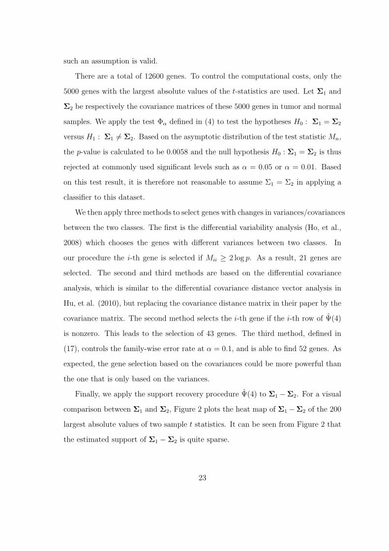
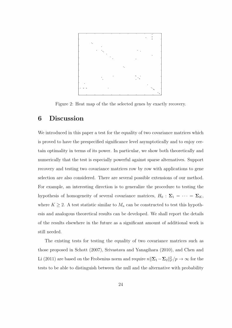
Finally, we apply the support recovery procedure Ψ(4) to Σ1 −Σ2. For a visual

comparison between Σ1 and Σ2, Figure 2 plots the heat map of Σ1 −Σ2 of the 200

largest absolute values of two sample t statistics. It can be seen from Figure 2 that

the estimated support of Σ1 −Σ2 is quite sparse.

23

20

40

60

80

100

120

140

160

180

200

Figure 2: Heat map of the the selected genes by exactly recovery.

6 Discussion

We introduced in this paper a test for the equality of two covariance matrices which

is proved to have the prespecified significance level asymptotically and to enjoy cer-

tain optimality in terms of its power. In particular, we show both theoretically and

numerically that the test is especially powerful against sparse alternatives. Support

recovery and testing two covariance matrices row by row with applications to gene

selection are also considered. There are several possible extensions of our method.

For example, an interesting direction is to generalize the procedure to testing the

hypothesis of homogeneity of several covariance matrices, H0 : Σ1 = · · · = ΣK ,

where K ≥ 2. A test statistic similar to Mn can be constructed to test this hypoth-

esis and analogous theoretical results can be developed. We shall report the details

of the results elsewhere in the future as a significant amount of additional work is

still needed.

The existing tests for testing the equality of two covariance matrices such as

those proposed in Schott (2007), Srivastava and Yanagihara (2010), and Chen and

Li (2011) are based on the Frobenius norm and require n∥Σ1−Σ2∥2F/p → ∞ for the

tests to be able to distinguish between the null and the alternative with probability

24

tending to 1. These tests are not suited for testing sparse alternatives. If Σ1−Σ2 is

a sparse matrix and the number of nonzero entries of Σ1−Σ2 is of order o(p/ log p)

and their magnitudes are of order C√log p/n, then it can be shown that the powers

of these tests are trivial. This fact was also illustrated in some of the simulation

results given in Section 5.

Much recent attention has focused on the estimation of large covariance and

precision matrices. The current work here is related to the estimation of covariance

matrices. An adaptive thresholding estimator of sparse covariance matrices was

introduced in Cai and Liu (2011). The procedure is based on the standardized

statistics σij/θ1/2ij , which is closely related to Mij. In this paper, the asymptotic

distribution of Mn = max1≤i≤j≤p Mij is obtained. It gives an justification on the

family-wise error of simultaneous tests H0ij : σij1 = σij2 for 1 ≤ i ≤ j ≤ p. For

example, by thresholding Mij at level 4 log p − log log p + qα, the family-wise error

is controlled asymptotically at level α, i.e.

FWER = P(

max(i,j)∈G

Mij ≥ 4 log p− log log p+ qα

)→ α,

where G = (i, j) : σij1 = σij2 and Card(Gc) = o(p2). These tests are useful in the

studies of differential coexpression in genetics; see de la Fuentea (2010).

7 Proofs

In this section, we will prove the main results. The proofs of Propositions 1-3 are

given in the supplementary material Cai, Liu and Xia (2011). Throughout this

section, we denote by C, C1, C2, . . ., constants which do not depend on n, p and

may vary from place to place. We begin by collecting some technical lemmas that

will be used in the proofs of the main results. These technical lemmas are proved

in the supplementary material, Cai, Liu and Xia (2011).

25

7.1 Technical lemmas

The first lemma is the classical Bonferroni’s inequality.

Lemma 1 (Bonferroni inequality) Let B = ∪pt=1Bt. For any k < [p/2], we have

2k∑t=1

(−1)t−1Et ≤ P(B) ≤2k−1∑t=1

(−1)t−1Et,

where Et =∑

1≤i1<···<it≤p P(Bi1 ∩ · · · ∩Bit).

The second lemma comes from Berman (1962).

Lemma 2 [Berman (1962)] If X and Y have a bivariate normal distribution with

expectation zero, unit variance and correlation coefficient ρ, then

limc→∞

P(X > c, Y > c

)[2π(1− ρ)1/2c2]−1 exp

(− c2

1+ρ

)(1 + ρ)1/2

= 1,

uniformly for all ρ such that |ρ| ≤ δ, for any δ, 0 < δ < 1.

The next lemma is on the large deviations for θij1 and θij2.

Lemma 3 Under the conditions of (C2) or (C2∗), there exists some constant C > 0

such that

P(maxi,j

|θij1 − θij1|/σii1σjj1 ≥ Cεnlog p

)= O(p−1 + n−ϵ/8), (18)

and

P(maxi,j

|θij2 − θij2|/σii2σjj2 ≥ Cεnlog p

)= O(p−1 + n−ϵ/8), (19)

where εn = max((log p)1/6/n1/2, (log p)−1) → 0 as n, p → ∞.

Define

Σ1 = (σij1)p×p =1

n1

n1∑k=1

(X − µ1)(X − µ1)T ,

Σ2 = (σij2)p×p =1

n2

n2∑k=1

(Y − µ2)(Y − µ2)T .

Let Λ be any subset of (i, j) : 1 ≤ i ≤ j ≤ p and |Λ| =Card(Λ).

26

Lemma 4 Under the conditions of (C2) or (C2∗), we have for some constant C > 0

that

P(max(i,j)∈Λ

(σij1 − σij2 − σij1 + σij2)2

θij1/n1 + θij2/n2

≥ x2)≤ C|Λ|(1− Φ(x)) +O(p−1 + n−ϵ/8)

uniformly for 0 ≤ x ≤ (8 log p)1/2 and Λ ⊆ (i, j) : 1 ≤ i ≤ j ≤ p.

The proofs of Lemmas 3 and 4 are given in the supplementary material Cai, Liu

and Xia (2011).

7.2 Proof of Theorem 1

Without loss of generality, we assume that µ1 = 0, µ2 = 0, σii1 = σii2 = 1 for

1 ≤ i ≤ p. Instead of the boundedness condition on the eigenvalues, we shall prove

the theorem under the more general condition that for any γ > 0, maxj sj = O(pγ),

where

sj := cardi : |ρij1| ≥ (log p)−1−α0 or |ρij2| ≥ (log p)−1−α0

with some α0 > 0. (Note that λmax(R1) ≤ C0 and λmax(R1) ≤ C0 implies that

maxj sj ≤ C(log p)2+2α0 .) Let

Mn = max1≤i≤j≤p

(σij1 − σij2)2

θij1/n1 + θij2/n2

, Mn = max1≤i≤j≤p

(σij1 − σij2)2

θij1/n1 + θij2/n2

.

Note that under the event |θij1/θij1 − 1| ≤ Cεn/ log p, |θij2/θij2 − 1| ≤ Cεn/ log p,

we have∣∣∣Mn − Mn

∣∣∣ ≤ CMnεnlog p

,∣∣∣Mn − Mn

∣∣∣ ≤ C(n1 + n2)(max1≤i≤p

X4i + max

1≤i≤pY 4i ) + C(n1 + n2)

1/2M1/2n (max

1≤i≤pX2

i + max1≤i≤p

Y 2i ).

By the exponential inequality, max1≤i≤p |Xi|+max1≤i≤p |Yi| = OP(√

log p/n). Thus,

by Lemma 3, it suffices to show that for any x ∈ R,

P(Mn − 4 log p+ log log p ≤ x

)→ exp

(− 1√

8πexp

(− x

2

))(20)

27

as n, p → ∞. Let ρij = ρij1 = ρij2 under H0. Define

Aj =i : |ρij| ≥ (log p)−1−α0

,

A = (i, j) : 1 ≤ i ≤ j ≤ p,

A0 = (i, j) : 1 ≤ i ≤ p, i ≤ j, j ∈ Ai,

B0 = (i, j) : i ∈ Λ(r), i < j ≤ p ∪ (i, j) : j ∈ Λ(r), 1 ≤ i < j,

D0 = A0 ∪B0.

By the definition of D0, for any (i1, j1) ∈ A \ D0 and (i2, j2) ∈ A \ D0, we have

|ρkl| ≤ r for any k = l ∈ i1, j1, i2, j2. Set

MA\D0 = max(i,j)∈A\D0

(σij1 − σij2)2

θij1/n1 + θij2/n2

, MD0 = max(i,j)∈D0

(σij1 − σij2)2

θij1/n1 + θij2/n2

.

Let yp = x+ 4 log p− log log p. Then∣∣∣P(Mn ≥ yp

)− P

(MA\D0 ≥ yp

)∣∣∣ ≤ P(MD0 ≥ yp

).

Note that Card(Λ(r)) = o(p) and for any γ > 0, maxj sj = O(pγ). This implies that

Card(D0) ≤ C0p1+γ + o(p2) for any γ > 0. By Lemma 4, we obtain that for any

fixed x ∈ R,

P(MD0 ≥ yp

)≤ Card(D0)× Cp−2 + o(1) = o(1).

Set

MA\D0 = max(i,j)∈A\D0

(σij1 − σij2)2

θij1/n1 + θij2/n2

=: max(i,j)∈A\D0

U2ij,

where

Uij =σij1 − σij2√

θij1/n1 + θij2/n2

.

It is enough to show that for any x ∈ R,

P(MA\D0 − 4 log p+ log log p ≤ x

)→ exp

(− 1√

8πexp

(− x

2

))28

as n, p → ∞. We arrange the two dimensional indices (i, j) : (i, j) ∈ A \ D0 in

any ordering and set them as (im, jm) : 1 ≤ m ≤ q with q =Card(A \ D0). Let

n2/n1 ≤ K1 with K1 ≥ 1, θk1 = θikjk1, θk2 = θikjk2 and define

Zlk =n2

n1

(XlikXljk − σikjk1), 1 ≤ l ≤ n1,

Zlk = −(YlikYljk − σikjk2), n1 + 1 ≤ l ≤ n1 + n2,

Vk =1√

n22θk1/n1 + n2θk2

n1+n2∑l=1

Zlk,

Vk =1√

n22θk1/n1 + n2θk2

n1+n2∑l=1

Zlk,

where

Zlk = ZlkI|Zlk| ≤ τn − EZlkI|Zlk| ≤ τn,

and τn = η−18K1 log(p + n) if (C2) holds, τn =√n/(log p)8 if (C2∗) holds. Note

that

max(i,j)∈A\D0

U2ij = max

1≤k≤qV 2k .

We have, if (C2) holds, then

max1≤k≤q

1√n

n1+n2∑l=1

E|Zlk|I|Zlk| ≥ η−18K1 log(p+ n)

≤ C√n max

1≤l≤n1+n2

max1≤k≤q

E|Zlk|I|Zlk| ≥ η−18K1 log(p+ n)

≤ C√n(p+ n)−4 max

1≤l≤n1+n2

max1≤k≤q

E|Zlk| exp(η|Zlk|/(2K1))

≤ C√n(p+ n)−4,

and if (C2∗) holds, then

max1≤k≤q

1√n

n1+n2∑l=1

E|Zlk|I|Zlk| ≥√n/(log p)8

≤ C√n max

1≤l≤n1+n2

max1≤k≤q

E|Zlk|I|Zlk| ≥√n/(log p)8

≤ Cn−γ0−ϵ/8.

Hence we have

P(max1≤k≤q

|Vk − Vk| ≥ (log p)−1)

≤ P(max1≤k≤q

max1≤l≤n1+n2

|Zlk| ≥ τn

)29

≤ np max1≤j≤p

[P(X2

j ≥ τn/2)+ P

(Y 2j ≥ τn/2

)]= O(p−1 + n−ϵ/8). (21)

Note that∣∣∣ max1≤k≤q

V 2k − max

1≤k≤qV 2k

∣∣∣ ≤ 2 max1≤k≤q

|Vk| max1≤k≤q

|Vk − Vk|+ max1≤k≤q

|Vk − Vk|2. (22)

By (21) and (22), it is enough to prove that for any x ∈ R,

P(max1≤k≤q

V 2k − 4 log p+ log log p ≤ x

)→ exp

(− 1√

8πexp

(− x

2

))(23)

as n, p → ∞. By Bonferroni inequality (see Lemma 1), we have for any fixed integer

m with 0 < m < q/2,

2m∑d=1

(−1)d−1∑

1≤k1<···<kd≤q

P( d∩

j=1

Ekj

)≤ P

(max1≤k≤q

V 2k ≥ yp

)≤

2m−1∑d=1

(−1)d−1∑

1≤k1<···<kd≤q

P( d∩

j=1

Ekj

), (24)

where Ekj = V 2kj

≥ yp. Let Zlk = Zlk/(n2θk1/n1 + θk2)1/2 for 1 ≤ k ≤ q and

W l = (Zlk1 , . . . , Zlkd), for 1 ≤ l ≤ n1 + n2. Define |a|min = min1≤i≤d |ai| for any

vector a ∈ Rd. Then we have

P( d∩

j=1

Ekj

)= P

(∣∣∣n−1/22

n1+n2∑l=1

W l

∣∣∣min

≥ y1/2n

).

By Theorem 1 in Zaitsev (1987), we have

P(∣∣∣n−1/2

2

n1+n2∑l=1

W l

∣∣∣min

≥ y1/2n

)≤ P

(|N d|min ≥ y1/2p − ϵn(log p)

−1/2)

+c1d5/2 exp

(− n1/2ϵn

c2d3τn(log p)1/2

), (25)

where c1 > 0 and c2 > 0 are absolutely constants, ϵn → 0 which will be specified

later and N d =: (Nk1 , . . . , Nkd) is a d dimensional normal vector with EN d = 0 and

30

Cov(N d) =n1

n2Cov(W 1) + Cov(W n1+1). Recall that d is a fixed integer which does

not depend on n, p. Because log p = o(n1/5), we can let ϵn → 0 sufficiently slow such

that

c1d5/2 exp

(− n1/2ϵn

c2d3τn(log p)1/2

)= O(p−M) (26)

for any large M > 0. It follows from (24), (25) and (26) that

P(max1≤k≤q

V 2k ≥ yp

)≤

2m−1∑d=1

(−1)d−1∑

1≤k1<···<kd≤q

P(|N d|min ≥ y1/2p − ϵn(log p)

−1/2)+ o(1).(27)

Similarly, using Theorem 1 in Zaitsev (1987) again, we can get

P(max1≤k≤q

V 2k ≥ yp

)≥

2m∑d=1

(−1)d−1∑

1≤k1<···<kd≤q

P(|N d|min ≥ y1/2p + ϵn(log p)

−1/2)− o(1). (28)

Lemma 5 For any fixed integer d ≥ 1 and real number x ∈ R,

∑1≤k1<···<kd≤q

P(|N d|min ≥ y1/2p ± ϵn(log p)

−1/2)= (1 + o(1))

1

d!

( 1√8π

exp(−x

2))d.(29)

The proof of Lemma 5 is very complicated, and is given in the supplementary

material Cai, Liu and Xia (2011). Submitting (29) into (27) and (28), we can get

lim supn,p→∞

P(max1≤k≤q

V 2k ≥ yp

)≤

2m∑d=1

(−1)d−1 1

d!

( 1√8π

exp(−x

2))d

and

lim infn,p→∞

P(max1≤k≤q

V 2k ≥ yp

)≥

2m−1∑d=1

(−1)d−1 1

d!

( 1√8π

exp(−x

2))d

for any positive integer m. Letting m → ∞, we obtain (23). The theorem is proved.

31

7.3 Proof of the other theorems

Proof of Theorem 2. Recall that

M1n = max

1≤i≤j≤p

(σij1 − σij2 − σij1 + σij2)2

θij1/n1 + θij2/n2

.

By Lemmas 3 and 4,

P(M1

n ≤ 4 log p− 1

2log log p

)→ 1 (30)

as n, p → ∞. By Lemma 3, the inequalities

max1≤i≤j≤p

(σij1 − σij2)2

θij1/n1 + θij2/n2

≤ 2M1n + 2Mn (31)

and

max1≤i≤j≤p

(σij1 − σij2)2

θij1/n1 + θij2/n2

≥ 16 log p,

we obtain that

P(Mn ≥ qα + 4 log p− log log p

)→ 1

as n, p → ∞. The proof of Theorem 2 is complete.

Proof of Theorem 4 Let M denote the set of all subsets of 1, ..., p with cardi-

nality c0(p). Let m be a random subset of 1, ..., p, which is uniformly distributed

on M. We construct a class of Σ1, N = Σm, m ∈ M, such that

σij = 0 for i = j and σii − 1 = ρ1i∈m,

for i, j = 1, ..., p and ρ = c√

log p/n, where c > 0 will be specified later. Let Σ2 = I

and Σ1 be uniformly distributed on N . Let µρ be the distribution of Σ1 − I. Note

that µρ is a probability measure on ∆ ∈ S(c0(p)) : ∥∆∥2F = c0(p)ρ2, where

S(c0(p)) is the class of matrices with c0(p) nonzero entries. Let dP1(Xn,Y n) be

the likelihood function given Σ1 being uniformly distributed on N and

Lµρ := Lµρ(Xn,Y n) = Eµρ

(dP1(Xn,Y n)dP0(Xn,Y n)

),

32

where Eµρ(·) is the expectation on Σ1. By the arguments in Baraud(2002), page

595, it suffices to show that

EL2µρ

≤ 1 + o(1).

It is easy to see that

Lµρ = Em

( n∏i=1

1

|Σm|1/2exp

(− 1

2ZT

i (Ωm − I)Zi

)),

where Ωm = Σ−1m and Z1, ...,Zn are i.i.d multivariate normal vectors with mean

vector 0 and covariance matrix I. Thus,

EL2µρ

= E( 1(

pkp

) ∑m∈M

( n∏i=1

1

|Σm|12

exp(− 1

2ZT

i (Ωm − I)Zi

)))2

=1(pkp

)2 ∑m,m′∈M

E( n∏

i=1

1

|Σm|12

1

|Σm′| 12exp

(− 1

2ZT

i (Ωm +Ωm′ − 2I)Zi

))).

Set Ωm + Ωm′ − 2I = (aij). Then aij = 0 for i = j, ajj = 0 if j ∈ (m ∪ m′)c,

ajj = 2( 11+ρ

− 1) if j ∈ m ∩ m′ and ajj = 11+ρ

− 1 if j ∈ m \ m′ and m′ \ m. Let

t = |m ∩m′|. Then we have

EL2µρ

=1(pkp

) kp∑t=0

(kpt

)(p− kpkp − t

)1

(1 + ρ)kpn(1 + ρ)(kp−t)n

(1 + ρ

1− ρ

)tn/2

≤ pkp(p− kp)!/p!

kp∑t=0

(kpt

)(kpp

)t( 1

1− ρ2

)tn/2

= (1 + o(1))(1 +

kpp(1− ρ2)n/2

)kp,

for r < 1/2. So

EL2µρ

≤ (1 + o(1)) exp(kp log(1 + kpp

c2−1))

≤ (1 + o(1)) exp(k2pp

c2−1)

= 1 + o(1)

by letting c be sufficiently small. Theorem 4 is proved.

33

Proof of Theorem 5. The proof of Theorem 5 is similar to that of Theorem 2. In

fact, by (30) and a similar inequality as (31), we can get

P(

min(i,j)∈Ψ

Mij ≥ 4 log p)→ 1 (32)

uniformly for (Σ1,Σ2) ∈ W0(4).

Proof of Theorem 6. Let A1 be the largest subset of 1, · · · , p \ 1 such that

σ1k1 = σ1k2 for all k ∈ A1. Let i1 = minj : j ∈ A1, j > 1. Then we have

|i1 − 1| ≤ s0(p). Also, Card(A1) ≥ p− s0(p). Similarly, let Al be the largest subset

of Al−1 \ il−1 such that σil−1k1 = σil−1k2 for all k ∈ Al and il = minj : j ∈ Al, j >

il−1. We can see that il− il−1 ≤ s0(p) for l < p/s0(p) and Card(Al) ≥Card(Al−1)−

s0(p) ≥ p − (s0(p) + 1)l. Let l = [pτ2 ] with τ/4 < τ2 < τ1. Let Σ1l and Σ2l be the

covariance matrices of (Xi0 , . . . , Xil) and (Yi0 , . . . , Yil). Then the entries of Σ1l and

Σ2l are the same except for the diagonal. Hence by the proof of Theorem 1, we can

show that

P(

max0≤j<k≤l

Mijik − 4 log l + log log l ≤ x)→ exp

(− 1√

8πexp

(− x

2

))uniformly for all Σ1 −Σ2 ∈ S0. This implies that

infΣ1−Σ2∈S0

P(

max0≤j<k≤l

Mijik ≥ c log p)→ 1

for all τ < c < 4τ2. By the definition of Ψ(τ) and the fact σijik1 = σijik2 for all

0 ≤ j < k ≤ l, Theorem 6 is proved.

References

[1] Anderson, T.W. (2003), An introduction to multivariate statistical analysis.

Third edition. Wiley-Interscience.

34

[2] Berman, S.M. (1962), Limiting distribution of the maximum term in sequences

of dependent random variables. The Annals of Mathematical Statistics, 33, 894-

908.

[3] Cai, T. and Jiang, T. (2011), Limiting laws of coherence of random matri-

ces with applications to testing covariance structure and construction of com-

pressed sensing matrices. The Annals of Statistics, 39, 1496-1525.

[4] Cai, T. and Liu, W.D. (2011), Adaptive thresholding for sparse covariance

matrix estimation. Journal of the American Statistical Association, 106, 672-

684.

[5] Cai, T., Liu, W.D. and Xia, Y. (2011), Supplement to “Two-sample covariance

matrix testing and support recovery”. Technical report.

[6] Chen, S. and Li, J. (2011), Two sample tests for high dimensional covariance

matrices. Technical report.

[7] de la Fuente, A. (2010), From “differential expression” to “differential

networking”-identification of dysfunctional regulatory networks in diseases.

Trends in Genetics, 26, 326-333.

[8] Gupta, A. K. and Tang, J. (1984), Distribution of likelihood ratio statistic

for testing equality of covariance matrices of multivariate Gaussian models.

Biometrika, 71, 555-559.

[9] Gupta, D.S. and Giri, N. (1973), Properties of tests concerning covariance

matrices of normal distributions. The Annals of Statistics, 6, 1222-1224.

[10] Ho, J.W., Stefani, M., dos Remedios, C.G. and Charleston, M.A. (2008), Dif-

ferential variability analysis of gene expression and its application to human

diseases. Bioinformatics, 24, 390-398.

35

[11] Hu, R, Qiu, X. and Glazko, G. (2010), A new gene selection procedure based

on the covariance distance. Bioinformatics, 26, 348-354.

[12] Hu, R, Qiu, X., Glazko, G., Klevanov, L. and Yakovlev, A. (2009), Detecting

intergene correlation changes in microarray analysis: a new approach to gene

selection. BMC Bioinformatics, 10:20.

[13] Jiang, T. (2004), The asymptotic distributions of the largest entries of sample

correlation matrices. The Annals of Applied Probability, 14, 865-880.

[14] Liu, W., Lin, Z.Y. and Shao, Q.M. (2008), The asymptotic distribution and

Berry-Esseen bound of a new test for independence in high dimension with an

application to stochastic optimization. The Annals of Applied Probability, 18,

2337-2366.

[15] O’Brien, P.C. (1992), Robust procedures for testing equality of covariance ma-

trices. Biometrics, 48, 819-827.

[16] Perlman, M.D. (1980), Unbiasedness of the likelihood ratio tests for equality of

several covariance matrices and equality of several multivariate normal popu-

lations. The Annals of Statistics, 8, 247-263.

[17] Sugiura, N. and Nagao, H. (1968), Unbiasedness of some test criteria for the

equality of one or two covariance matrices. The Annals of Mathematical Statis-

tics, 39, 1682-1692.

[18] Schott, J. R. (2007), A test for the equality of covariance matrices when the

dimension is large relative to the sample sizes. Computational Statistics and

Data Analysis, 51, 6535-6542.

36

[19] Singh, D., Febbo, P., Ross, K., Jackson, D., Manola, J., Ladd, C., Tamayo, P.,

Renshaw, A., D′Amico, A. and Richie, J. (2002). Gene expression correlates of

clinical prostate cancer behavior. Cancer Cell, 1, 203-209.

[20] Srivastava, M. S. and Yanagihara, H. (2010), Testing the equality of several

covariance matrices with fewer observations than the dimension. Journal of

Multivariate Analysis, 101, 1319-1329.

[21] Xu, P., Brock, G.N. and Parrish, R.S. (2009), Modified linear discriminant anal-

ysis approaches for classification of high-dimensional microarray data. Compu-

tational Statistics and Data Analysis, 53, 1674-1687,

[22] Zaıtsev, A. Yu. (1987), On the Gaussian approximation of convolutions under

multidimensional analogues of S.N. Bernstein’s inequality conditions. Probabil-

ity Theory and Related Fields, 74, 535-566.

[23] Zhou, W. (2007), Asymptotic distribution of the largest off-diagonal entry of

correlation matrices. Transactions of the American Mathematical Society, 359,

5345-5364.

37