two-sample tests in functional data analysis starting from discrete data

Statistica Sinica 17(2007), 1511-1531

TWO-SAMPLE TESTS IN FUNCTIONAL DATA ANALYSIS

STARTING FROM DISCRETE DATA

Peter Hall1,2 and Ingrid Van Keilegom2

1The University of Melbourne and 2Universite catholique de Louvain

Abstract: One of the ways in which functional data analysis differs from other ar-

eas of statistics is in the extent to which data are pre-processed prior to analysis.

Functional data are invariably recorded discretely, although they are generally sub-

stantially smoothed as a prelude even to viewing by statisticians, let alone further

analysis. This has a potential to interfere with the performance of two-sample sta-

tistical tests, since the use of different tuning parameters for the smoothing step,

or different observation times or subsample sizes (i.e., numbers of observations per

curve), can mask the differences between distributions that a test is trying to lo-

cate. In this paper, and in the context of two-sample tests, we take up this issue.

Ways of pre-processing the data, so as to minimise the effects of smoothing, are

suggested. We show theoretically and numerically that, by employing exactly the

same tuning parameter (e.g. bandwidth) to produce each curve from its raw data,

significant loss of power can be avoided. Provided a common tuning parameter is

used, it is often satisfactory to choose that parameter along conventional lines, as

though the target was estimation of the continuous functions themselves, rather

than testing hypotheses about them. Moreover, in this case, using a second-order

smoother (such as a local-linear method), the subsample sizes can be almost as

small as the square root of sample sizes before the effects of smoothing have any

first-order impact on the results of a two-sample test.

Key words and phrases: Bandwidth, bootstrap, curve estimation, hypothesis test-

ing, kernel, Cramer-von Mises test, local-linear methods, local-polynomial methods,

nonparametric regression, smoothing.

1. Introduction

Although, in functional data analysis, the data are treated as though they

are in the form of curves, in practice they are invariably recorded discretely.

They are subject to a pre-processing step, usually based on local-polynomial or

spline methods, to transform them to the smooth curves to which the familiar

algorithms of functional data analysis are applied. In many instances the pre-

processing step is not of great importance. However, in the context of two-sample

hypothesis testing it has the potential to significantly reduce power. Our aim in

the present paper is to explore this issue, and suggest methods which allow the

effects of smoothing to be minimised.

1512 PETER HALL AND INGRID VAN KEILEGOM

Although smoothing methods are sometimes used in related contexts, for

example to produce alternatives to traditional two-sample hypothesis tests, there

the mathematical models with which a statistician typically works allow for the

discrete, unprocessed form of the data. See, for example, Dette and Neumeyer

(2001). Moreover, in such instances the data are passed from one statistician to

another before processing, i.e., before smoothing.

By way of contrast, functional datasets are usually exchanged by researchers

in post-processed form, after the application of a smoothing algorithm; that is

seldom the case for data in related problems such as nonparametric regression.

The widespread use of pre-process smoothing for functional data makes the ef-

fects of smoothing more insidious than usual, and strengthens motivation for

understanding the impact that smoothing might have.

There is rightly a debate as to whether statistical smoothing should be used

at all, in a conventional sense, when constructing two-sample hypothesis tests.

Employing a small bandwidth (in theoretical terms, a bandwidth which converges

to zero as sample size increases) can reduce statistical power unnecessarily, al-

though from other viewpoints power can be increased. See, for example, the dis-

cussion by Ingster (1993), Fan (1994), Anderson, Hall and Titterington (1994),

Fan (1998), Fan and Ullah (1999) and Li (1999).

It has also been observed, in a range of settings, that when probability

statements rather than Lp metrics are to be optimised, undersmoothing can give

improved performance. In particular, the level accuracy of tests can be improved

by undersmoothing; see, for example, Hall and Sheather (1988), Koenker and

Machado (1999) and Koenker and Xiao (2002).

In the context of two-sample hypothesis testing, our main recommendation is

appropriate in cases where the “subsample sizes” (that is, the numbers of points

at which data are recorded for individual functions) do not vary widely. There

we suggest that exactly the same tuning parameters be used to produce each

curve from its raw data, for all subsamples in both datasets. For example, when

using kernel-based methods this would mean using the same bandwidth in all

cases; for splines it would mean using the same penalty, or the same knots. Such

a choice ensures that, under the null hypothesis that the two samples of curves

come from identical populations, the main effects of differing observation-time

distributions and differing subsample sizes (for the different curves) cancel. As a

result, the effect that smoothing has on bias is an order of magnitude less than

it would be if different bandwidths, tuned to the respective curves, were used.

The latter approach can lead to power loss for a two-sample test.

The fact that the common tuning parameter can be chosen by a conventional

curve-estimation method, such as cross-validation or a plug-in rule, is an attrac-

tive feature of the proposal. New smoothing-parameter choice algorithms are not

TESTS FOR FUNCTIONAL DATA 1513

essential. Nevertheless, it can be shown that under more stringent assumptions

a bandwidth of smaller size can be advantageous. See Sections 3.3 and 4, and

also Hall and Van Keilegom (2006), for discussion.

In a more general setting, where k samples are available and our task is to

test the null hypothesis that all are identical, a test is typically constructed by

taking either the weighted sum, or the maximum, of values of a statistic Tj1j2 that

tests for differences between populations j1 and j2. However, if the test leads to

rejection, then one generally seeks further information about differences among

populations that pairwise tests can provide. For these reasons, the conclusions

we reach for two-sample hypothesis tests have direct implications for k-sample

problems.

Recent work on two-sample hypothesis tests in nonparametric and semipara-

metric settings includes that of Louani (2000), Claeskens, Jing, Peng and Zhou

(2003) and Cao and Van Keilegom (2006). Extensive discussion of methods and

theory for functional data analysis is given by Ramsay and Silverman (1997,

2002). Recent contributions to hypothesis testing in this field include those

of Fan and Lin (1998), Locantore, Marron, Simpson, Tripoli, Zhang and Cohn

(1999), Spitzner, Marron and Essick (2003), Cuevas, Febrero and Fraiman (2004)

and Shen and Faraway (2004). However, this work does not broach the subject

of the effect that pre-processing has on results.

2. Statement of Problem and Methodology

2.1. The data and the problem.

We observe data

Uij =Xi(Sij) + δij , 1 ≤ i ≤ m, 1 ≤ j ≤ mi ,(2.1)

Vij = Yi(Tij) + ǫij , 1 ≤ i ≤ n , 1 ≤ j ≤ ni ,

where X1,X2, . . . are identically distributed as X; Y1, Y2, . . . are identically dis-

tributed as Y ; the δij ’s are identically distributed as δ; the ǫij ’s are identically

distributed as ǫ; X and Y are both random functions, defined on the inter-

val I = [0, 1]; the observation errors, δij and ǫij , have zero means and uni-

formly bounded variances; the sequences of observation times, Si1, . . . , Simiand

Ti1, . . . , Tini, are either regularly spaced on I or drawn randomly from a distri-

bution (possibly different for each i, and also for S and T ) having a density that

is bounded away from zero on I; and the quantities Xi1 , Yi2 , Si1j1 , Ti2j2 , δi1 and

ǫi2, for 1 ≤ i1 ≤ m, 1 ≤ j1 ≤ mi1, 1 ≤ i2 ≤ n and 1 ≤ j2 ≤ ni2, are all totally

independent.

Given the data at (2.1), we wish to test the null hypothesis, H0, that the

distributions of X and Y are identical. In many cases of practical interest, X and


Y would be continuous with probability 1, and then H0 would be characterised

by the statement,

FX(z) = FY (z) for all continuous functions z ,

where FX and FY are the distributional functionals of X and Y , respectively:

FX(z) = P{X(t) ≤ z(t) for all t ∈ I

},

FY (z) = P{Y (t) ≤ z(t) for all t ∈ I

}.

Thus, our approach to analysis will focus on differences between distribu-

tions, rather than (for instance) on differences between means, of random func-

tions. However, conclusions similar to those discussed here would be drawn in

the context of testing hypotheses about a mean. Issues connected with equality

of distributions are increasingly of interest even in parametric settings, for exam-

ple in connection to the fitting of models (e.g., the equilibrium-search model of

Mortensen (1990) and Burdett and Mortensen (1998)) to wage and employment

data. In such problems, goodness of fit can be addressed by drawing a very large

(effectively, infinite) sample from the population defined by the model with pa-

rameters fitted, and applying a two-sample test in the context of those data and

the sample that is being compared with the model.

In some problems, the time points Sij and Tij would be regularly spaced on

grids of the same size. For example, they might represent the times of monthly

observations of a process, such as the number of tons of a certain commodity

exported by a particular country in month j of year i, in which case mi = ni = 12

for each i. (The differing lengths of different months could usually be ignored. In

examples such as this we might wish first to correct the data for linear or periodic

trends.) Here the assumption of independence might not be strictly appropriate,

but the methods that we suggest will be approximately correct under conditions

of weak dependence.

In other cases the values of mi and ni can vary from one index i to another,

and in fact those quantities might be modelled as conditioned values of random

variables. The observation times may also exhibit erratic variation. For example,

in longitudinal data analysis, Uij might represent a measurement of the condition

of the ith type-X patient at the jth time in that patient’s history. Since patients

are seen only at times that suit them, then both the values of the observation

times, and the number of those times, can vary significantly from patient to

patient.

In general, unless we have additional knowledge about the distributions of

X and Y (for example, both distributions are completely determined by finite

parameter vectors), we cannot develop a theoretically consistent test unless the


values of mi and ni increase without bound as m and n increase. Therefore, the

divergence of mi and ni will be a key assumption in our theoretical analysis.

2.2. Methodology for testing hypotheses

Our approach to testing H0 is to compute estimators, Xi and Yi, of Xi

and Yi, by treating the problem as one of nonparametric regression and passing

nonparametric smoothers through the datasets (Si1, Ui1), . . . , (Simi, Uimi

) and

(Ti1, Vi1), . . . , (Tini, Vini

), respectively. Then, treating the functions X1, . . . , Xm

and Y1, . . . , Yn as independent and identically distributed observations of X and

Y , respectively (under our assumptions they are at least independent), we con-

struct a test of H0.

For example, we might compute estimators FX and FY of FX and FY , re-

spectively:

FX(z) =1

m

m∑

i=1

I(Xi ≤ z

), FY (z) =

1

n

n∑

i=1

I(Yi ≤ z

), (2.2)

where the indicator I(Xi ≤ z) is interpreted as I{Xi(t) ≤ z(t) for all t ∈ I},

and I(Yi ≤ z) is interpreted similarly. These quantities might be combined into

a test statistic of Cramer-von Mises type, say

T =

∫ {FX(z) − FY (z)

}2µ(dz) , (2.3)

where µ denotes a probability measure on the space of continuous functions.

An alternative approach would be to use, rather than T , a Kolmogorov-

Smirnov statistic, T ′ = supz |FX (z) − FY (z)|. However, this would typically

produce a test with less power than a test founded on T , since for the latter

statistic the differences between the two distribution functions are averaged over

all z values for which they arise, rather than just in the vicinity of the value of

z for which the distance is greatest.

The integral in (2.3) can be calculated by Monte Carlo simulation, for ex-

ample as

TN =1

N

N∑

i=1

{FX(Mi) − FY (Mi)

}2, (2.4)

whereM1, . . . ,MN are independent random functions with the distribution ofM ,

say, for which µ(A) = P (M ∈ A) for each Borel set A in the space of continuous

functions on I. Of course, the Mi’s are independent of FX and FY , and TN → T ,

with probability one conditional on the data, as N → ∞. Note that in the latter

result, T does not depend on N .


2.3. Methodology for estimating Xi and Yi

For brevity we confine attention to just one technique, local-polynomial

methods, for computing Xi and Yi. (Results can be expected to be similar if one

uses other conventional smoothers, for example splines.) Taking the degree of the

polynomial to be odd, and estimating Xi, we compute the value (a0, . . . , a2r+1)

of the vector (a0, . . . , a2r+1) that minimises

mi∑

j=1

{Uij −

2r−1∑

k=0

ak (Sij − t)k}2

K

(t− Sij

hXi

),

where r ≥ 1 is an integer, hXi is a bandwidth, and K, the kernel function, is

a bounded, symmetric, compactly supported probability density. Then, a0 =

Xi(t).

In the particular case r = 1 we obtain a local-linear estimator of Xi(t),

Xi(t) =Ai2(t)Bi0(t) −Ai1(t)Bi1(t)

Ai0(t)Ai2(t) −Ai1(t)2,

where

Air(t) =1

mihXi

mi∑

j=1

(t− Sij

hXi

)r

K

(t− Sij

hXi

),

Bir(t) =1

mihXi

mi∑

j=1

Uij

(t− Sij

hXi

)r

K

(t− Sij

hXi

),

hXi denotes a bandwidth and K is a kernel function. The estimator Yi is con-

structed similarly. Local-linear methods have an advantage over higher-degree

local-polynomial approaches in that they suffer significantly less from difficulties

arising from singularity, or near-singularity, of estimators.

Treating Xi as a fixed function (that is, fixing i and conditioning on the

stochastic process Xi), assuming that Xi has 2(r + 1) bounded derivatives, and

that hXi is chosen of size m−1/(2r+1)i , the estimator Xi converges to Xi at the

mean-square optimal rate m−2r/(2r+3)i , as mi increases. See, for example, Fan

(1993), Fan and Gijbels (1996) and Ruppert and Wand (1994) for discussion of

both practical implementation and theoretical issues.

2.4. Bandwidth choice

A number of potential bandwidth selectors are appropriate when all the

subsample sizes mi and nj are similar and the bandwidths h = hXi = hY j are

identical. Theoretical justification for using a common bandwidth, when the goal

is hypothesis testing rather than function estimation, will be given in Section 3.


One approach to common bandwidth choice is to use a “favourite” methodto compute an empirical bandwidth for each curve Xi and Yj, and then take theaverage value to be the common bandwidth. Another technique, appropriate in

the case of plug-in rules, is to use an average value of each of the components ofa plug-in bandwidth selector, and assemble the average values, using the plug-informula, to form the common bandwidth. A third approach, valid in the context

of cross-validation, is to use a criterion which is the average of the cross-validatorycriteria corresponding to the different curves. For each of these methods, “av-erage” might be defined in a weighted sense, where the weights represent therespective subsample sizes.

2.5. Bootstrap calibration

Bootstrap calibration is along conventional lines, as follows. Having con-structed smoothed estimators Xi and Yi of the functions Xi and Yi, respectively,

pool them into the class

Z = {Z1, . . . , Zm+n} ={X1, . . . , Xm

}∪

{Y1, . . . , Yn

}. (2.5)

By sampling randomly, with replacement, from Z, derive two independent re-samples {X∗

1 , . . . ,X∗m} and {Y ∗

1 , . . . , Y∗n }; compute

F ∗X(z) =

1

m

m∑

i=1

I(X∗

i ≤ z), F ∗

Y (z) =1

n

n∑

i=1

I(Y ∗

i ≤ z);

and finally, calculate

T∗

=

∫ {F ∗

X(z) − F ∗Y (z)

}2µ(dz) . (2.6)

Of course, F ∗X and F ∗

Y are bootstrap versions of the actual empirical distri-bution functionals,

FX(z) =1

m

m∑

i=1

I(Xi ≤ z

), FY (z) =

1

n

n∑

i=1

I(Yi ≤ z

), (2.7)

which we would have computed if we had access to the full-function data Xi

and Yi. Likewise, T is the ideal, but impractical, test statistic that we wouldhave used if we had those data:

T =

∫ {FX(z) − FY (z)

}2µ(dz) . (2.8)

Suppose the desired critical level for the test is 1−α. By repeated resamplingfrom Z we can compute, by Monte Carlo means, the critical point, tα say, givenby

P(T∗≥ tα

∣∣ Z)

= α . (2.9)


We reject the null hypothesis H0, that there is no difference between the distri-

butions of X and Y , if T > tα.

At this point, some of the potential difficulties of two-sample hypothesis

testing become clear. Regardless of how we smooth the data, the conditional

expected value of F ∗X − F ∗

Y , given Z, is exactly zero. However, even if H0 is cor-

rect, E(FX − FY ) will generally not vanish, owing to the different natures of the

datasets providing information about the functions Xi and Yi (for example, dif-

ferent distributions of the sampling times), and the different ways we constructed

Xi and Yi from those data. Therefore, the test statistic T suffers biases which

are not reflected in its bootstrap form, T∗, and which can lead to loss of power

for the test. Of course, this problem would vanish if we could use FX − FY in

place of FX − FY for the test; that is, if we could employ T instead of T . But in

practice, that is seldom possible.

2.6. Choice of the measure µ

Recall from (2.4) that our application of the measure µ, to calculate the

statistic T , proceeds by simulating the stochastic process M of which µ defines

the distribution. Therefore it is necessary only to construct M . It is satisfactory

to define M in terms of its Karhunen-Loeve expansion,

M(t) = γ(t) +

∞∑

i=1

ζi φi(t) ,

where γ(t) = E{M(t)}, the functions φi form a complete orthonormal sequence

on I, and the random variables ζi are uncorrelated and have zero mean.

We take ζi = θi ξi, where θ1 > θ2 > . . . > 0 are positive constants decreasing

to zero, and the random variables ξi are independent and identically distributed

with zero means and unit variances. The functions φi could be chosen to be the

orthonormal functions corresponding to a principal component analysis of the

dataset Z at (2.5). In this case they would form the sequence of eigenvectors of

a linear operator, the kernel of which is the function

L(s, t) =1

m+ n

m+n∑

i=1

{Zi(s) − Z(s)} {Zi(t) − Z(t)} ,

where Z = (m+ n)−1∑

i≤m+n Zi. The constants θi would in that case be given

by the square-root of the corresponding eigenvalues.

However, exposition is simpler if we take the φi’s to be a familiar orthonormal

sequence, such as the cosine sequence on I:

φ1 ≡ 1 , φi+1(x) = 212 cos(iπx) for i ≥ 1 .


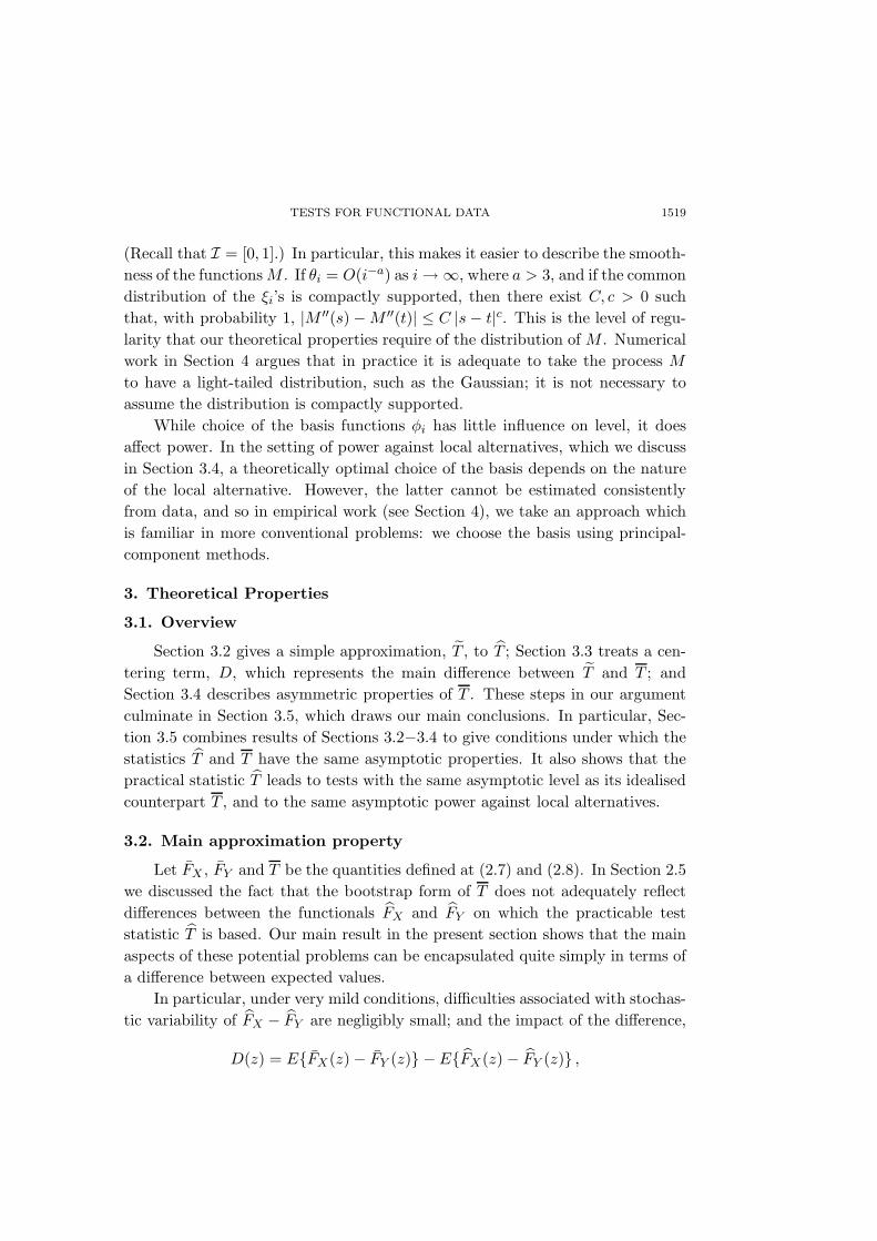
(Recall that I = [0, 1].) In particular, this makes it easier to describe the smooth-

ness of the functionsM . If θi = O(i−a) as i→ ∞, where a > 3, and if the common

distribution of the ξi’s is compactly supported, then there exist C, c > 0 such

that, with probability 1, |M ′′(s) −M ′′(t)| ≤ C |s− t|c. This is the level of regu-

larity that our theoretical properties require of the distribution of M . Numerical

work in Section 4 argues that in practice it is adequate to take the process M

to have a light-tailed distribution, such as the Gaussian; it is not necessary to

assume the distribution is compactly supported.

While choice of the basis functions φi has little influence on level, it does

affect power. In the setting of power against local alternatives, which we discuss

in Section 3.4, a theoretically optimal choice of the basis depends on the nature

of the local alternative. However, the latter cannot be estimated consistently

from data, and so in empirical work (see Section 4), we take an approach which

is familiar in more conventional problems: we choose the basis using principal-

component methods.

3. Theoretical Properties

3.1. Overview

Section 3.2 gives a simple approximation, T , to T ; Section 3.3 treats a cen-

tering term, D, which represents the main difference between T and T ; and

Section 3.4 describes asymmetric properties of T . These steps in our argument

culminate in Section 3.5, which draws our main conclusions. In particular, Sec-

tion 3.5 combines results of Sections 3.2−3.4 to give conditions under which the

statistics T and T have the same asymptotic properties. It also shows that the

practical statistic T leads to tests with the same asymptotic level as its idealised

counterpart T , and to the same asymptotic power against local alternatives.

3.2. Main approximation property

Let FX , FY and T be the quantities defined at (2.7) and (2.8). In Section 2.5

we discussed the fact that the bootstrap form of T does not adequately reflect

differences between the functionals FX and FY on which the practicable test

statistic T is based. Our main result in the present section shows that the main

aspects of these potential problems can be encapsulated quite simply in terms of

a difference between expected values.

In particular, under very mild conditions, difficulties associated with stochas-

tic variability of FX − FY are negligibly small; and the impact of the difference,

D(z) = E{FX(z) − FY (z)} − E{FX (z) − FY (z)} ,


can be summarised very simply. Theorem 1 below shows that T is closely ap-

proximated by

T =

∫ {FX(z) − FY (z) −D(z)

}2µ(dz) . (3.1)

The sets of assumptions A.1 and A.2, used for Theorems 1 and 2 respectively,

will be collected together in Section 5. Proofs of the results are given in

Hall and Van Keilegom (2006).

Theorem 1. If the measure µ has no atoms, and assumption A.1 holds, then

∣∣T 12 − T

12

∣∣ = op

(m− 1

2 + n−12). (3.2)

To interpret this result, note that, under the null hypothesis the distributions

of X and Y are identical, T is of size m−1+n−1. (Further discussion of this point

is given in Section 3.4.) The quantity, D(z), can only increase this size. Result

(3.2) asserts that the difference between T 1/2 and T 1/2 is actually of smaller

order than the asymptotic sizes of either T 1/2 or T 1/2, and so D(z) captures all

the main issues that will affect the power and level accuracy of the statistic T ,

compared with those of T .

3.3. Properties of D(z)

First we summarise properties of D(z) when (2r − 1)st degree local-

polynomial estimators are employed. Using arguments similar to those in

Hall and Van Keilegom (2006), it may be shown that for functions z that are

sufficiently smooth, and for each η > 0,

P(Xi ≤ z

)= P (Xi ≤ z) +O

{h2r−η

Xi + (mihXi)η−1

}. (3.3)

This result, and its analogue for the processes Yi and Yi, lead to the following

result. Under the null hypothesis, and for each η > 0,

D(z) = O

[1

m1−η

m∑

i=1

{h2r

Xi+(mihXi)−1

}+

1

n1−η

n∑

j=1

{h2r

Y j+(njhY j)−1

}]. (3.4)

Neglecting the effects of η, assuming that the subsample sizes mi and ni are

close to a common value ν, say, and supposing that the bandwidths hXi and hY j

are also taken of similar sizes, (3.4) suggests allowing those bandwidths to be of

size ν−1/(2r+1). Then D(z) = O(ν−2r/(2r+1)).

While this approach is of interest, the extent of reduction in subsampling

effects under H0 can often be bettered by taking the bandwidths h = hXi = hY j

to be identical, all 1 ≤ i ≤ m and 1 ≤ j ≤ n. This allows the quantities

that contribute the dominant bias terms, involving h2rXi and h2r

Y j in (3.3) and


their analogues for the Y -sample, to cancel perfectly. That reduces the bias

contribution, from the 2rth to the 2(r + 1)st power of bandwidth.

Using identical bandwidths makes local-linear methods, which correspond

to taking r = 1 in the formulae above, particularly attractive for at least two

reasons. First, the contribution of bias is reduced to that which would arise

through fitting third-degree, rather than first-degree, polynomials in the case

of non-identical bandwidths, yet the greater robustness of first-degree fitting

is retained. Secondly, the appropriate bandwidth is now close to ν−1/5, the

conventional bandwidth size for estimating the functions Xi and Yi as functions

in their own right. This suggests that tried-and-tested bandwidth selectors, such

as those discussed in Section 2.4, could be used.

The mathematical property behind the common-bandwidth recommendation

is the following more detailed version of (3.3), which for simplicity we give only

in the local-linear case, i.e., r = 1. If h = hXi for each i and h is of size ν−1/5,

or larger, then for each η > 0,

P(Xi ≤ z

)= P

(Xi + 1

2 κ2 h2X ′′

i ≤ z)

+O{h4−η + (νh)η−1

}(3.5)

uniformly in smooth functions z, where κ2 =∫u2K(u) du. If H0 holds, and we

use the bandwidth h for the Y data as well as for the X data, then

P(Xi + 1

2 κ2 h2X ′′

i ≤ z)

= P(Yi + 1

2 κ2 h2 Y ′′

i ≤ z)

(3.6)

for each i and each function z. Therefore (3.5) implies that, under H0 and

assuming that the subsample sizes are all similar to ν,

P(Xi ≤ z

)− P

(Yj ≤ z

)= O

{h4−η + (νh)η−1

}

for 1 ≤ i ≤ m and 1 ≤ j ≤ n.

Optimising the right-hand side of (3.6) with respect to h suggests using

a relatively conventional bandwidth selector of size ν−1/5. A small value of the

right-hand side of (3.6) implies that D is close to zero, which in turn ensures that

T (which is close to T , as shown in Section 3.2) is well-approximated by T . Such

a result implies that the bootstrap test is unlikely to reject H0 simply because of

poor choice of smoothing parameters; see Section 5.2 for further discussion.

We conclude with a concise statement of (3.5). Given sequences am and bmof positive numbers, write am ≍ bm to denote that am/bm is bounded away from

zero and infinity as n→ ∞. The reader is referred to Section 5.2 for a statement

of assumption A.2 for Theorem 2. It includes the condition that all bandwidths

h = hXi are identical, and h ≍ ν−1/q where 3 < q <∞.


Theorem 2. If r = 1 and A.2 holds then for each η > 0,

P(Xi ≤ z

)− P

(Xi + 1

2 κ2 h2X ′′

i ≤ z)

=

O(ν

η− (q−1)2

4q ) if 3 < q ≤ 5

O(νη− 4

q ) if q > 5,

(3.7)

where the “big oh” terms are of the stated orders uniformly in functions z that

have two Holder-continuous derivatives, and for 1 ≤ i ≤ m.

3.4. Asymptotic distribution of T , and power

If m and n vary in such a way that

m

n→ ρ ∈ (0,∞) as m→ ∞ , (3.8)

and if, as prescribed by H0, the distributions of X and Y are identical, then T

satisfies

mT → ζ ≡

∫ {ζX(z) − ρ

12 ζY (z)

}2µ(dz) . (3.9)

Here the convergence is in distribution, and ζX(z) and ζY (z) are independent

Gaussian processes with zero means and the same covariance structures as the

indicator processes I(X ≤ z) and I(Y ≤ z), respectively. In particular, the

covariance of ζX(z1) and ζX(z2) is FX(z1 ∧ z2) − FX(z1)FX(z2).

It follows directly from (3.9) that the asymptotic value of the critical point for

an α-level test of H0, based on T , is the quantity uα such that P (ζ > uα) = α.

Analogously, the critical point tα for the bootstrap statistic T∗

(see (2.6) and

(2.9)) converges, after an obvious rescaling, to uα as sample size increases: under

H0,

P (mT > uα) → α , m tα → uα , (3.10)

where the second convergence is in probability. Of course, these are conventional

properties of bootstrap approximations. In Section 3.5 we discuss conditions that

are sufficient for the practical test statistic T , rather than its ideal form T , to

have asymptotically correct level; see (3.17).

Power properties under local alternatives are also readily derived. In partic-

ular, if FY is fixed and

FX(z) = FY (z) +m− 12 c δ(z) , (3.11)

where δ is a fixed function and c is a constant, then with convergence interpreted

in distribution,

mT →

∫ {ζY 1(z) + c δ(z) − ρ

12 ζY 2(z)

}2µ(dz) , (3.12)


of which (3.9) is a special case. In (3.12), ζY 1 and ζY 2 are independent Gaussian

processes each with zero mean and the covariance structure of ζY .

From this result and the second part of (3.10) it is immediate that, provided

δ is not almost surely zero with respect to µ measure, a test based on the ideal

statistic T , but using the bootstrap critical point tα, is able to detect departures

proportional to m−1/2 δ:

limc→∞

lim infm→∞

Pc

(T > tα

)= 1 , (3.13)

where Pc denotes probability under the model where FY is fixed and FX is given

by (3.11). In Section 3.5 we note that if we use a common bandwidth, and if the

subsample sizes are not too much smaller than the sample sizes m and n, then

the same result holds true for T .

Proofs of (3.9), (3.10) and (3.12) are straightforward. They do not require

convergence of function-indexed empirical processes to Gaussian processes, and

proceed instead via low-dimensional approximations to those empirical processes.

3.5. Sufficient conditions for T and T to have identical asymptotic

distributions under H0

Assume (3.8) and the conditions of Theorem 2 for both the X and Y popu-

lations, and in particular that all the subsample sizes mi and ni are of the same

order in the sense that

ν ≍ min1≤i≤m

mi ≍ max1≤i≤m

mi ≍ min1≤i≤n

ni ≍ max1≤i≤n

ni (3.14)

as m,n → ∞. Take h ≍ ν−1/5. Then Theorem 2, and its analogue for the Y

sample, imply that under H0,

D(z) = O(νη− 4

5)

(3.15)

uniformly in functions z with two Holder-continuous derivatives, for each η > 0.

Theorem 1 implies that, in order for the practical statistic T , and its “ideal”

version T , to have identical asymptotic distributions, it is necessary only that

D(z) be of smaller order than the stochastic error of FX − FY . Equivalently, if

(3.8) holds, D(z) should be of smaller order than m−1/2, uniformly in functions

z with two Holder-continuous derivatives. For that to be true it is sufficient, in

view of (3.15), that

m = O(ν

85−η

)(3.16)

for some η > 0.

It follows from (3.10) that, provided (3.16) holds and the null hypothesis is

correct,

P(mT > uα

)→ α . (3.17)


This is the analogue of the first part of (3.10) for T rather than its ideal form T .

Similarly, (3.13) holds for T rather than T , if a common bandwidth is used and

the subsample sizes satisfy (3.14). This confirms the ability of the practicable

test, based on T , to detect semiparametric departures from the null hypothesis.

Condition (3.16) is surprisingly mild. It asserts that, in order for the effects

of estimating Xi and Yi to be negligible, it is sufficient that the subsample sizes

mi and ni be of larger order than the 5/8th root of the smaller of the two sample

sizes, m and n.

4. Numerical Properties

Suppose that Sij (1 ≤ i ≤ m; 1 ≤ j ≤ mi) are i.i.d. uniform on [0, 1] and

that Tij (1 ≤ i ≤ n; 1 ≤ j ≤ ni) are i.i.d. with density 2 − b + 2(b − 1)t for

0 ≤ t ≤ 1 and 0 < b < 2. Note that this last density reduces to the uniform

density when b = 1. We take b = 1.2. The errors δij and ǫij are independent and

come from a normal distribution with mean zero and standard deviation σ = 0.1

and 0.3, respectively. Suppose that X1, . . . ,Xm are identically distributed as X,

where X(t) =∑

k≥1 ck NkX ψk(t), ck = e−k/2, NkX (k ≥ 1) are i.i.d. standard

normal random variables and ψk(t) = 21/2 sin{(k− 1)πt} (k > 1) and ψ1 ≡ 1 are

orthonormal basis functions. Similarly, let Y1, . . . , Yn be identically distributed

as Y , where

Y (t) =

∞∑

k=1

ck NkY 1 ψk(t) + a

∞∑

k=1

ak NkY 2 ψ∗k(t) .

Here NkY 1 and NkY 2 are i.i.d. standard normal variables, a ≥ 0 controls the

deviation from the null model (a = 0 under H0), ak = k−2, and

ψ∗k(t) =

1 if k = 1

212 sin{(k − 1)π(2t − 1)} if k is odd and k > 1

212 cos{(k − 1)π(2t − 1)} if k is even

are orthonormal basis functions. For practical reasons, we truncate the infinite

sum in the definition of X(t) and Y (t) at k = 15. Define Uij = Xi(Sij) + δij(1 ≤ i ≤ m; 1 ≤ j ≤ mi) and Vij = Yi(Tij) + ǫij (1 ≤ i ≤ n; 1 ≤ j ≤ ni).

Finally, M1, . . . ,MN are independent and have the same distribution asM , where

M(t) =∑

k≥1 ckNkZ φk(t), NkZ are i.i.d. standard normal variables, and φk(t) =

21/2 cos{(k − 1)πt} (k > 1) and φ1 ≡ 1 are orthonormal functions. We take

N = 50 and truncate the infinite sum after 15 terms. The simulation results

are based on 500 samples, and the critical values of the test are obtained from

250 bootstrap samples. The functions X(t) and Y (t) are estimated by means of


local-linear smoothing. The bandwidth is chosen to minimise the cross-validation

type criterion

1

mim

m∑

i=1

mi∑

j=1

{Uij − X−(j)i (Sij)}

2 +1

ni n

n∑

i=1

ni∑

j=1

{Vij − Y−(j)i (Tij)}

2 ,

where X−(j)i is the estimated regression curve without using observation j (and

similarly for Y−(j)i ). The functionK is the biquadratic kernel, K(u) = (15/16)(1−

u2)2I(|u| ≤ 1).

The results for m = n = 15, 25, 50 and m1 = n1 = 20 and 100 are sum-

marised in Figure 1. The level of significance is α = 0.05 and is indicated in the

figure. The graphs show that under the null hypothesis the level is well respected

and that the power increases for larger values of m,n,m1, n1 and a. The value

of the subsample sizes m1 and n1 has limited impact on the power, whereas this

is clearly not the case for the sample sizes m and n. Other settings that are

not reported here (equal variances in the two populations, bigger sample and

subsample sizes, ...) show similar behavior for the power curves.

Figure 1. Rejection probabilities for m = n = 15 (full curve), m = n = 25

(dashed curve) and m = n = 50 (dotted curve). The thin curves correspond

to m1 = n1 = 20, the thick curves to m1 = n1 = 100. The null hypothesis

holds for a = 0.

In Section 3.3 we explained why it is recommended to take hXi = hY j = h.

We now verify in a small simulation study that identical bandwidths indeed lead

to higher power. Consider the same model as above, except that now the standard


deviations of the errors δij and ǫij are 0.2 and 0.5, respectively. Take m = n = 15,

25, and 50, m1 = 20 and n1 = 100. Figure 2 shows the power curves for this

model. The rejection probabilities are obtained using either identical bandwidths

(estimated by means of the above cross-validation procedure), or using different

bandwidths for each sample (estimated by means of a cross-validation procedure

for each sample). The graph suggests that under H0 the empirical level is close

to the nominal level in both cases. The power is, however, considerably lower

when different bandwidths are used than when the same bandwidth is used for

both samples. The differences in power, for different bandwidths, are not so

marked when the values of m1 and n1 are similar, but in such cases there is little

motivation for taking the bandwidths to be quite different.

Figure 2. ejection probabilities for m = n = 15 (full curve), m = n = 25

(dashed curve) andm = n = 50 (dotted curve). The thin curves are obtained

by using different bandwidths for each sample, the thick curves use the same

bandwidth. In all cases, m1 = 20 and n1 = 100. The null hypothesis holds

for a = 0.

Finally, we apply the proposed method to temperature data collected by 224

weather stations across Australia (see Hall and Tajvidi (2002)). The data set

consists of monthly average temperatures in degrees Celcius. The starting year

of the registration of these data depends on the weather station and varies from

1856 to 1916. Data were registered until 1993. Figure 3 shows the temperature

curves of the 224 weather stations during 1990. We restrict attention to the

curves between 1914 and 1993, in order to have complete data information for

(almost) all weather stations. We are interested in whether weather patterns


in Australia have changed during this time period. To test this hypothesis, we

split the time interval in 4 periods of equal length, namely from 1914 to 1933

(period 1), from 1934 to 1953 (period 2), from 1954 to 1973 (period 3) and from

1974 to 1993 (period 4), and execute the proposed pairwise tests on each of the

six possible pairs. Curves containing missing monthly temperature values are

eliminated from the analysis.

Figure 3. Temperature curves for the 224 weather stations in 1990.

We obtain the optimal bandwidth for each combination of two periods by

means of the above cross-validation procedure. In each case we find h = 2.2.

Next, we need to determine an appropriate measure µ or, equivalently, an ap-

propriate process M . For this, we follow the procedure described in Section 2.6:

let φi(t) and θ2i be the eigenfunctions and eigenvalues corresponding to a prin-

cipal component analysis (PCA) of the dataset, and truncate the infinite sum

at four terms. The variables ξi (1 ≤ i ≤ 4) are taken as independent standard

normal variables, and the mean function γ(t) is estimated empirically. The esti-

mation of these functions is carried out by using the PCA routines available on

J. Ramsay’s homepage (http://ego.psych.mcgill.ca/misc/fda/). Next, based on

the so-obtained process M , we calculate the test statistics for each comparison

and approximate the corresponding p-values from 1,000 resamples. The p-values

are summarized in Table 1. At the 5% level, two comparisons (period 1 versus

3 and period 3 versus 4) lead to non-significant p-values (although borderline),

all other p-values are significant: the data suggest that the average climate in

Australia has changed over time.


Table 1. P -values of the pairwise tests for the Australian weather data.

Period Period P -value

1 2 0.0011 3 0.081

1 4 0.024

2 3 0.001

2 4 0.0003 4 0.053

5. Assumptions for Section 3

5.1. Conditions for Theorem 1

The assumptions are the following, comprising A.1: for some η > 0,

min(

min1≤i≤m

mi, min1≤i≤n

ni

)→ ∞ , (5.1)

max1≤i≤m

hXi+ max1≤j≤n

hY j → 0, min1≤i≤m

(m1−η

i hXi

)+ min

1≤j≤n

(n1−η

j hY j

)→ ∞, (5.2)

K is a bounded, symmetric, compactly-supported probability density, (5.3)

the observation times Sij and Tij are independent random vari-

ables, identically distributed for each i, and with densities that are

bounded away from zero uniformly in i and in population type.

(5.4)

Assumption (5.1) asks that the subsample sizes mi and ni diverge to infinity

in a uniform manner as m and n grow. This is a particularly mild condition; wedo not expect a subsample to provide asymptotically reliable information about

the corresponding random functions, Xi or Yi, unless it is large. The first part

of (5.2) asks that the bandwidths hXi and hY j be uniformly small. Again thisis a minimal condition, since bandwidths that converge to zero are necessary for

consistent estimation of Xi and Yi. Likewise, the second part of (5.2) is only alittle stronger than the assumption that the variances of the estimators of Xi and

Yi decrease uniformly to zero.

Assumptions (5.3) and (5.4) are conventional. The latter is tailored to thecase of random design, as too is (5.9) below; in the event of regularly spaced

design, both can be replaced by simpler conditions.

5.2. Conditions for Theorem 2

We need the following notation. Given C > 0 and r ∈ (1, 2], write Cr(C)

for the class of differentiable functions, z, on I for which: (a) ‖z′‖∞ ≤ C; (b) if1 < r < 2, |z′(s)− z′(t)| ≤ C |s− t|r−1 for all s, t ∈ I; and (c) if r = 2, z has two

bounded derivatives and ‖z′′‖∞ ≤ C. Given d > 0, put Wd = X + dX ′′, where

X denotes a generic Xi, and let fWd(s) denote the probability density of Wd(s).

CONSERVATIVE, NONPARAMETRIC ESTIMATION 1529

The assumptions leading to Theorem 2 are the following, comprising A.2:

the kernelK is a symmetric, compactly-supported probability den-

sity with two Holder-continuous derivatives;(5.5)

ν ≍ min1≤i≤m

mi ≍ max1≤i≤m

mi as m→ ∞ ; (5.6)

for some 0 < η < 1 and all sufficiently large m, mη ≤ ν ≤ m1/η; (5.7)

the common bandwidth, h = hXi, satisfies,

for some η > 0 , h ≍ ν−1/q where 3 < q <∞ ; (5.8)

the respective densities fi of the observation times Sij satisfy,

sup1≤i<∞

supt∈I

|f ′′i (t)| <∞ , inf1≤i<∞

inft∈I

fi(t) > 0 ; (5.9)

the random function X has four bounded derivatives, with

E(|δ|s

)<∞ , E

{supt∈I

maxr=1,...,4

∣∣X(r)(t)∣∣s

}<∞ for each s > 0 ; (5.10)

sup|d|≤c

sups∈I

∥∥fWd(s)

∥∥∞<∞ for some c > 0 ; (5.11)

for 1 ≤ p ≤ 2 and c > 0, and for each C > 0,

P (Wd ≤ z + y) = P (Wd ≤ z) +

∫

Iy(s)P

{Wd ≤ z

∣∣ Wd(s) = z(s)}

(5.12)×fWd(s){z(s)} ds +O

(‖y‖p

∞

),

uniformly in z ∈ C2(C), in y ∈ Cp(C), and in d satisfying |d| ≤ c.

Conditions (5.5)−(5.11) are conventional. A proof of (5.12), in the case p = 2

and under the assumption that W ′′ is well-defined and continuous, is given in

Hall and Van Keilegom (2006).

Acknowledgements

We are grateful to two reviewers for helpful comments. The research of Van

Keilegom was supported by IAP research network grant nr. P5/24 of the Belgian

government (Belgian Science Policy).

References

Anderson, N. H., Hall, P. and Titterington, D. M. (1994). Two-sample test statistics for measur-

ing discrepancies between two multivariate probability density functions using kernel-based

density estimates. J. Multivariate Anal. 50, 41-54.

Burdett, K. and Mortensen, D. T. (1998). Wage differentials, employer size, and unemployment.

Internat. Econ. Rev. 39, 257-273.


Cao, R. and Van Keilegom, I. (2006). Empirical likelihood tests for two-sample problems via

nonparametric density estimation. Canad. J. Statist., 34, 61-77.

Claeskens, G., Jing, B.-Y., Peng, L. and Zhou, W. (2003). Empirical likelihood confidence

regions for comparison distributions and ROC curves. Canad. J. Statist. 31, 173-190.

Cuevas, A., Febrero, M. and Fraiman, R. (2004). An anova test for functional data. Comput.

Statist. Data Anal. 47, 111-122.

Dette, H. and Neumeyer, N. (2001). Nonparametric analysis of covariance. Ann. Statist. 29,

1361-1400.

Fan, J. (1993). Local linear regression smoothers and their minimax efficiencies. Ann. Statist.

21, 196-216.

Fan, J. and Gijbels, I. (1996). Local Polynomial Modelling and its Applications. Chapman and

Hall, London.

Fan, J. and Lin, S.-K. (1998). Test of significance when data are curves. J. Amer. Statist. Assoc.

93, 1007-1021.

Fan, Y. Q. (1994). Testing the goodness-of-fit of a parametric density-function by kernel method.

Econom. Theory 10, 316-356.

Fan, Y. Q. (1998). Goodness-of-fit tests based on kernel density estimators with fixed smoothing

parameter. Econom. Theory 14, 604-621.

Fan, Y. Q. and Ullah, A. (1999). On goodness-of-fit tests for weakly dependent processes using

kernel method. J. Nonparametr. Statist. 11, 337-360.

Hall, P. and Sheather, S. J. (1988). On the distribution of a Studentized quantile. J. Roy. Statist.

Soc. Ser. B 50, 381-391.

Hall, P. and Tajvidi, N. (2002). Permutation tests for equality of distributions in high-

dimensional settings. Biometrika 89, 359-374.

Hall, P. and Van Keilegom, I. (2006). Two-sample tests in functional data analysis from discrete

data. http://www3.stat.sinica.edu.tw/statistica.

Ingster, Y. I. (1993). Asymptotically minimax hypothesis testing for nonparametric alternatives.

I, II. Math. Methods Statist. 2, 85-114, 171-189.

Li, Q. (1999). Nonparametric testing the similarity of two unknown density functions: Local

power and bootstrap analysis. J. Nonparametr. Statist. 11, 189-213.

Koenker, R. and Machado, J. A. F. (1999). Goodness of fit and related inference processes for

quantile regression. J. Amer. Statist. Assoc. 94, 1296-1310.

Koenker, R. and Xiao, Z. J. (2002). Inference on the quantile regression process. Econometrica

70, 1583-1612.

Locantore, N., Marron, J. S., Simpson, D. G., Tripoli, N., Zhang, J. T. and Cohn, K. L. (1999).

Robust principal component analysis for functional data (with discussion). Test 8, 1-73.

Louani, D. (2000). Exact Bahadur efficiencies for two-sample statistics in functional density

estimation. Statist. Decisions 18, 389-412.

Mortensen, D. T. (1990). Equilibrium wage distributions: A synthesis. In Panel Data and Labor

Market Studies (Edited by Joop Hartog, Geert Ridder and Jules Theeuwe), 279-96. North-

Holland, Amsterdam.

Ramsay, J. O. and Silverman, B. W. (1997). Functional Data Analysis. Springer, New York.

Ramsay, J. O. and Silverman, B. W. (2002). Applied Functional Data Analysis: Methods and

Case Studies. Springer, New York.

CONSERVATIVE, NONPARAMETRIC ESTIMATION 1531

Ruppert, D. and Wand, M. P. (1994). Multivariate locally weighted least squares regression.

Ann. Statist. 22, 1346-1370.

Shen, Q. and Faraway, J. (2004). An F test for linear models with functional responses. Statist.

Sinica 14, 1239-1257.

Spitzner, D. J., Marron, J. S. and Essick, G. K. (2003). Mixed-model functional ANOVA for

studying human tactile perception. J. Amer. Statist. Assoc. 98, 263-272.

Department of Mathematics and Statistics, The University of Melbourne, Melbourne, VIC 3010,

Australia.

E-mail: [email protected]

Institut de Statistique, Universite catholique de Louvain, Voie du Roman Pays 20, B-1348

Louvain-la-Neuve, Belgium.

E-mail: [email protected]

(Received August 2005; accepted March 2006)

Documents

two-sample tests in functional data analysis starting from discrete data