1

Two-stage informative cluster sampling - estimation and prediction Abdulhakeem Eideh1 Alquds University, Palestine Gad Nathan Hebrew University of Jerusalem, Israel

Ray Chambers

University of Southampton, UK

Summary. The aims of this article are twofold: first estimate the parameters of the superpopulation model for two-stage cluster sampling from a finite population when the sampling design for the both stages is informative. Second predict the finite population total, cluster-specific effects for clusters in the sample and clusters not in the sample, and predict the cluster totals for clusters in the sample and clusters not in the sample. To achieve this we derive the sample and complement-sample distributions and the moments of the first stage and second stage measurements. Also we derive the conditional sample and conditional sample-complement distributions and the moments of the cluster-specific effects given the cluster measurements. Keywords: Analysis of variance; Empirical best linear unbiased predictor; Informative sampling; Pseudo maximum likelihood; Sample distribution. 1. Introduction Two-stage cluster sampling is frequently used in health and social sciences. Classical theory underlying the use of this sampling mechanism involves simple random sampling for each of the two stages or unequal probabilities of selection at one or more of the two stages- see Cochran (1977), Sarndal, Swensson, and Wretman (1997), and Lohr (1999) for discussion and examples. In such cases the relationship between the response variable and the covariates in the sample is the same as modeled for the population. When the selection probabilities are related to the values of the response variable even after conditioning on concomitant variables included in the population model, we obtain what is known as informative sampling, which results in selection bias, consequently the relationship between the response variable and the covariates in the sample differs from the population model, so that standard estimates of the population model parameters severely biased, leading possibly to false inference-for more discussion, see Pfeffermann, Krieger and Rinott (1998). In a recent master thesis Amin (2000) consider the estimation of the variance components model parameters when the sampling design for the first stage is informative with exponential sampling while for the second stage is noninformative. In (2001) Pfeffermann, Moura and Silva estimate the parameters of the two-level model under informative sampling design for both stages using the Markov Chain Monte Carlo algorithm. The authors noted that the sample models used for this experiment are correct. In practice the relationship between the sample selection probabilities and the model dependent variables need to be identified from the sample. 1 Address for correspondence: Department of Mathematics, Faculty of Science and Technology, Alquds University, Abu-Dies Campus, Palestine , P.O. Box 20002, East Jerusalem,

2

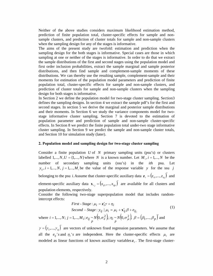
Neither of the above studies considers maximum likelihood estimation method, prediction of finite population total, cluster-specific effects for sample and non-sample clusters, and prediction of cluster totals for sample and non-sample clusters when the sampling design for any of the stages is informative. The aims of the present study are twofold: estimation and prediction when the sampling design for the both stages is informative. Special cases are those in which sampling at one or neither of the stages is informative. In order to do that we extract the sample distributions of the first and second stages using the population model and first order inclusion probabilities, extract the sample marginal and sample posterior distributions, and then find sample and complement-sample moments of these distributions. We can thereby use the resulting sample, complement-sample and their moments for estimation of the population model parameters and prediction of finite population total, cluster-specific effects for sample and non-sample clusters, and prediction of cluster totals for sample and non-sample clusters when the sampling design for both stages is informative. In Section 2 we define the population model for two-stage cluster sampling. Section3 defines the sampling designs. In section 4 we extract the sample pdf’s for the first and second stages. In section 5 we derive the marginal and posterior sample distributions and their moments. In Section 6 we study the variance components model for two-stage informative cluster sampling. Section 7 is devoted to the estimation of population parameter and prediction of sample and non-sample cluster-specific effects. In Section 8 we predict the finite population total under-two stage informative cluster sampling. In Section 9 we predict the sample and non-sample cluster totals, and Section 10 for simulation study (later). 2. Population model and sampling design for two-stage cluster sampling Consider a finite population U of N primary sampling units (psu’s) or clusters labelled },...,1{ ,,...,1 NUN = where N is a known number. Let NiM i ,...,1 , = be the number of secondary sampling units (ssu’s) in the ith psu. Let

iij MjNiy ,...,1 ,,...,1 , == be the value of the response variable y for the ssu j

belonging to the psu .i Assume that cluster-specific auxiliary data ( )′= iqii zz ,...,1z and

element-specific auxiliary data ( )′= ijpijji xx ,...,1x are available for all clusters and population elements, respectively. Consider the following two-stage superpopulation model that includes random-intercept effects:

, |::-

ijijiiij

iiieyStageSecond

StageFirst+′+=−

+′=

βµµ

ηγµ

xz

(1)

where ( ) ( ) ( )′=== pp

iep

iji NNeMjNi βββσησ µ ,..., ,,0~ ;,,0~ ;,...,1 ;,...,1 122 and

( ) ,...,1′

= qγγγ are vectors of unknown fixed regression parameters. We assume that all the ' and ' sse iij η are independent. Here the cluster-specific effects iµ are modeled as linear functions of known auxiliary variables iz . The first-stage cluster-

3

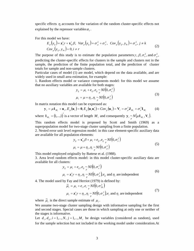
specific effects iη accounts for the variation of the random cluster-specific effects not explained by the repressor variables iz . For this model we have:

( ) ( ) ( )( ) ,0,

,, , , 222

riyyCovkjyyCovyVaryE

rkijp

ikijpeijpijiijp

≠=

≠=+=′+′=µµ

σσσβγ xz (2)

The purpose of this study is to estimate the population parameters 22 and , , ,µ

σσβγ e , predicting the cluster-specific effects for clusters in the sample and clusters not in the sample, the prediction of the finite population total, and the prediction of cluster totals for sample and non-sample clusters. Particular cases of model (1) are model, which depend on the data available, and are widely used in small area estimation, for example: 1. Random effects model or variance components model: for this model we assume that no auxiliary variables are available for both stages:

( )

( )2

2

,0~,

,0~,

µσηηµµ

σµ

NI

NIeey

piii

epijijiij

+=

+=

(3)

In matrix notation this model can be expressed as: ( ) ( ) ( )

iii MeMiipiipipiMi CovEE IJVuuu0uu1y 22, , σσµµ

+===′=+= (4)

where ( )′= 1,...,1iM1 is a vector of length iM and consequently ( )iMpi i

N V1y ,~ µ .

This random effects model is proposed by Scott and Smith (1969) as a superpopulation model for two-stage cluster sampling from a finite population. 2. Nested error unit level regression model: in this case element-specific auxiliary data are available for all population elements:

( )

( )2

2

,0~,

,0~,

µσηηµµ

σµβ

NI

NIeey

piii

epijijiijij

+=

++′= x (5)

This model employed originally by Battese et al. (1988). 3. Area level random effects model: in this model cluster-specific auxiliary data are available for all clusters:

( )

( ) tindependen are and ,,0~,

,0~,

i2

2

ησηηγµ

σµ

µ ijpiiii

epijijiij

eNI

NIeey

+′=

+=

z (6)

4. The model used by Fay and Herriot (1979) is defined by: ( )

( ) tindependen are and ,,0~,

,0~,~

i2

2

ησηηγµ

σµµ

µ ipiiii

Dipiiii

eNI

NIee

+′=

+=

z (7)

where iµ~ is the direct sample estimate of iµ .

We assume two-stage cluster sampling design with informative sampling for the first and second stages. Special cases are those in which sampling at only one or neither of the stages is informative. Let iiji MjNidd ,...,1 ,,...,1 , , == be design variables (considered as random), used for the sample selection but not included in the working model under consideration.At

4

the first stage a sample s of size n psu’s (clusters) is selected with inclusion probabilities:

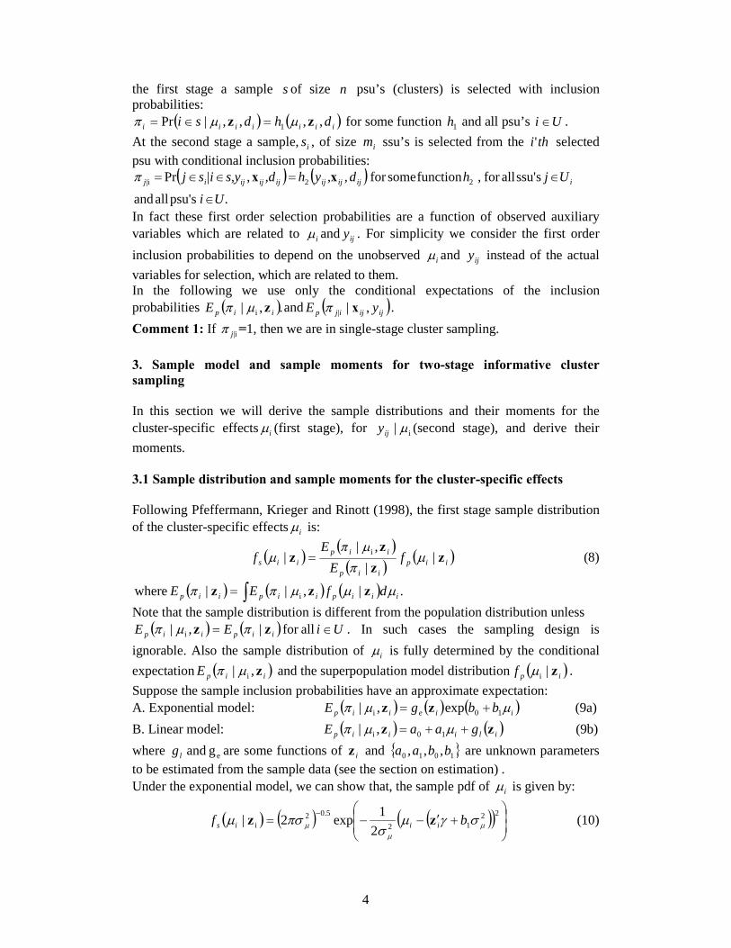
( ) ( )iiiiiii dhdsi ,,,,|Pr 1 zz µµπ =∈= for some function 1h and all psu’s Ui∈ . At the second stage a sample, is , of size im ssu’s is selected from the thi' selected psu with conditional inclusion probabilities:

( ) ( ).spsu' all and

sssu' allfor function somefor ,,Pr 22i|

U iU j , h d,yh,ds,y|isj iijijijijijijij

∈

∈=∈∈= xxπ

In fact these first order selection probabilities are a function of observed auxiliary variables which are related to iµ and ijy . For simplicity we consider the first order inclusion probabilities to depend on the unobserved iµ and ijy instead of the actual variables for selection, which are related to them. In the following we use only the conditional expectations of the inclusion probabilities ( ).,| i iipE zµπ and ( )ijijijp yE ,|| xπ . Comment 1: If i|jπ =1, then we are in single-stage cluster sampling. 3. Sample model and sample moments for two-stage informative cluster sampling In this section we will derive the sample distributions and their moments for the cluster-specific effects iµ (first stage), for i| µijy (second stage), and derive their moments. 3.1 Sample distribution and sample moments for the cluster-specific effects Following Pfeffermann, Krieger and Rinott (1998), the first stage sample distribution of the cluster-specific effects iµ is:

( )( )

( )( )iip

iip

iipiis f

EE

f zz

zz |

|,|

| iµ

π

µπµ = (8)

( ) ( ) ( ) .|,|| where i iiipiipiip dfEE µµµππ ∫= zzz Note that the sample distribution is different from the population distribution unless

( ) ( ) UiEE iipiip ∈= allfor |,| i zz πµπ . In such cases the sampling design is ignorable. Also the sample distribution of iµ is fully determined by the conditional expectation ( )iipE z,| iµπ and the superpopulation model distribution ( )ipf z|iµ . Suppose the sample inclusion probabilities have an approximate expectation: A. Exponential model: ( ) ( ) ( )iieiip bbgE µµπ 10i exp,| += zz (9a) B. Linear model: ( ) ( )iliiip gaaE zz ++= µµπ 10i ,| (9b) where eg and lg are some functions of iz and { } ,,, 1010 bbaa are unknown parameters to be estimated from the sample data (see the section on estimation) . Under the exponential model, we can show that, the sample pdf of iµ is given by:

( ) ( ) ( )( )

+′−−=

− 2212

5.02i 2

1exp2|µ

µ

µσγµ

σπσµ bf iiis zz (10)

5

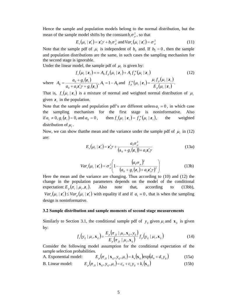
Hence the sample and population models belong to the normal distribution, but the mean of the sample model shifts by the constant 2

1 µσb , so that

( ) ( ) 221 and

µµσµσγµ =′|+′=′| iisiiis VarbE zzz (11)

Note that the sample pdf of iµ is independent of 0b and. If 01 =b , then the sample and population distributions are the same, in such cases the sampling mechanism for the second stage is ignorable. Under the linear model, the sample pdf of iµ is given by:

( ) ( ) ( )iiw

piipiis fAfAf zzz || | 10 µµµ +== (12)

where ( )( ) 01

i10

00 1 , AA

gaagaA

li

il−=

+′+

+=

zzz

γand ( )

( )

( )iip

piwp E

ff

zz

z||

| iiii

µ

µµµ = .

That is, ( )i| zisf µ is a mixture of normal and weighted normal distribution of iµ given iz in the population. Note that the sample and population pdf’s are different unless 01 =a , in which case the sampling mechanism for the first stage is noninformative. Also if ( ) 0 and 0, ,0 01 ==≠ aga il z , then ( ) ( )ii || zz i

wpis ff µµ = , the weighted

distribution of iµ . Now, we can show thatthe mean and the variance under the sample pdf of iµ in (12) are:

( )( )( ) γ

σγµ

µ

iiliiis ag

aE

zzzz

′+++′=′|

10

21

a

(13a)

( )( )( )( )

′++−=′| 2

10

212 1

γ

σσµ

µ

µ

iiliis aga

aVar

zzz (13b)

Here the mean and the variance are changing. Thus according to (10) and (12) the change in the population parameters depends on the model of the conditional expectation: ( )iipE z,| iµπ . Also note that, according to (13bb),

( ) ( )iipiis VarVar zz ′|≤′| µµ with equality if and if 01 =a , that is when the sampling design is noninformative. 3.2 Sample distribution and sample moments of second stage measurements Similarly to Section 3.1, the conditional sample pdf of igiven µijy and ijx is given by:

( )( )( )

( )ijiijpijiijp

ijijiijpijiijs yf

EyE

yf xx

xx ,|

,|,,|

,||

|µ

µπ

µπµ = (14)

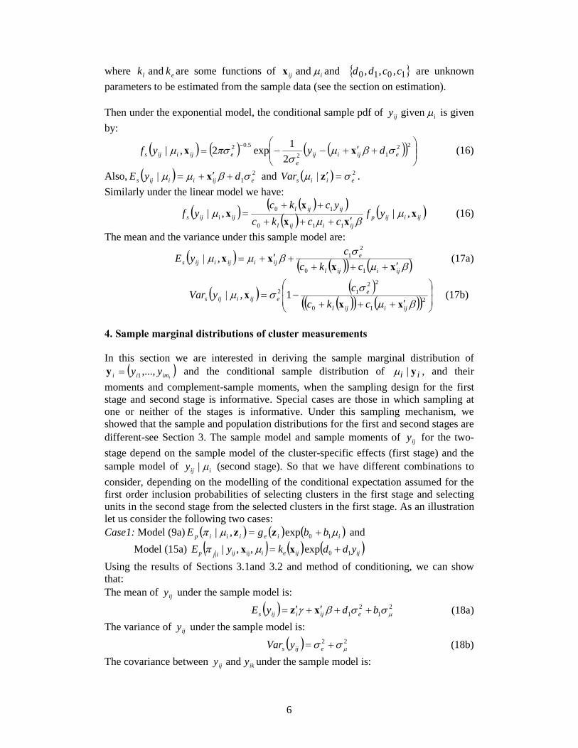
Consider the following model assumption for the conditional expectation of the sample selection probabilities. A. Exponential model: ( ) ( ) ( )ijijeiijijijp yddkyE 10| exp,,| += xx µπ (15a) B. Linear model: ( ) ( )ijlijiijijijp kyccyE xx ++= 10| ,,| µπ (15b)

6

where el kk and are some functions of iij µ and x and { }1010 ,,, ccdd are unknown parameters to be estimated from the sample data (see the section on estimation). Then under the exponential model, the conditional sample pdf of igiven µijy is given by:

( ) ( ) ( )( )

+′+−−=

− 2212

5.02

21exp2,| eijiij

eeijiijs dyyf σβµ

σπσµ xx (16)

Also, ( ) ( ) 221 and eiiseijiiijs VardyE σµσβµµ =′|+′+=| zx .

Similarly under the linear model we have:

( )( )( )

( )( )ijiijp

ijiijl

ijijlijijs yf

cckcyckc

yf xxx

xx ,|,|

110

10i µ

βµµ

′+++

++= (16)

The mean and the variance under this sample model are:

( )( )( ) ( )

,10

21

βµ

σβµµ

ijiijl

eijiijiijs ckc

cyE

xxxx

′++++′+=| (17a)

( ) ( )( )( ) ( )( )

′+++−=| 2

10

2212 1,

βµ

σσµ

ijiijl

eeijiijs ckc

cyVarxx

x (17b)

4. Sample marginal distributions of cluster measurements In this section we are interested in deriving the sample marginal distribution of

( )iimii yy ,...,1=y and the conditional sample distribution of ii y|µ , and their

moments and complement-sample moments, when the sampling design for the first stage and second stage is informative. Special cases are those in which sampling at one or neither of the stages is informative. Under this sampling mechanism, we showed that the sample and population distributions for the first and second stages are different-see Section 3. The sample model and sample moments of ijy for the two-stage depend on the sample model of the cluster-specific effects (first stage) and the sample model of i| µijy (second stage). So that we have different combinations to consider, depending on the modelling of the conditional expectation assumed for the first order inclusion probabilities of selecting clusters in the first stage and selecting units in the second stage from the selected clusters in the first stage. As an illustration let us consider the following two cases: Case1: Model (9a) ( ) ( ) ( )iieiip bbgE µµπ 10i exp,| += zz and Model (15a) ( ) ( ) ( )ijijeiijijp yddkyE 10ij exp,,| +=

xx µπ

Using the results of Sections 3.1and 3.2 and method of conditioning, we can show that: The mean of ijy under the sample model is:

( ) 21

21 µ

σσβγ bdyE eijiijs ++′+′= xz (18a) The variance of ijy under the sample model is:

( ) 22µ

σσ += eijs yVar (18b) The covariance between ikij yy and under the sample model is:

7

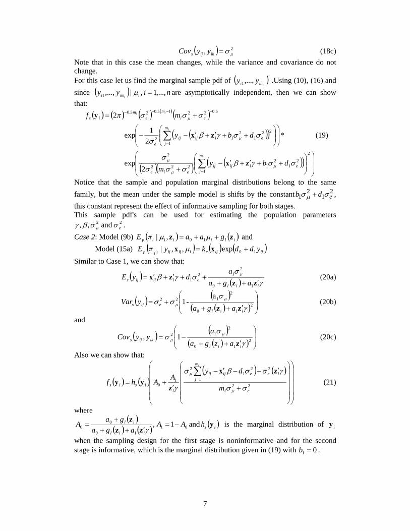
( ) , 2µ

σ=ikijs yyCov (18c) Note that in this case the mean changes, while the variance and covariance do not change. For this case let us find the marginal sample pdf of ( )

iimi yy ,...,1 .Using (10), (16) and since ( ) niyy iimi i

,...,1 ,|,...,1 =µ are asymptotically independent, then we can show that:

( ) ( ) ( ) ( )( )

( )( )

( )( )( )( )

++′+′−

+

++′+′−−

+=

∑

∑

=

=

−−−−

2

1

21

21222

2

1

221

212

5.02215.025.0

2exp

*2

1exp

2

i

i

ii

m

jeiijij

eie

m

jeiijij

e

eim

em

is

dbym

dby

mf

σσγβσσσ

σ

σσγβσ

σσσπ

µ

µ

µ

µ

µ

zx

zx

y

(19)

Notice that the sample and population marginal distributions belong to the same family, but the mean under the sample model is shifts by the constant 2

12

1 edb σσ µ + , this constant represent the effect of informative sampling for both stages. This sample pdf's can be used for estimating the population parameters

22 and ,, eσσβγµ

. Case 2: Model (9b) ( ) ( )iliiip gaaE zz ++= µµπ 10i ,| and Model (15a) ( ) ( ) ( )ijijeiijijp yddkyE 10ij exp,,| +=

xx µπ

Similar to Case 1, we can show that:

( )( ) γ

σσγβ

µ

iileiijijs aga

adyE

zzzx

′++++′+′=

10

212

1 (20a)

( )( )( )( )

′+++= 2

10

2122 a

-1 γ

σσσ

µ

µ

iileijs aga

yVarzz

(20b)

and

( )( )( )( )

′++−= 2

10

212 1,

γ

σσ

µ

µ

iilikijs azga

ayyCov

z (20c)

Also we can show that:

( ) ( )( ) ( )

+

′+−′−

′+=

∑=

221

221

2

10

ei

m

jieeijij

iisis m

dyAAhf

i

σσ

γσσβσ

γµ

µzx

zyy (21)

where ( )

( ) ( ) 0110

00 1 , AA

agagaA

iil

il−=

′++

+=

γzzz and ( )ish y is the marginal distribution of iy

when the sampling design for the first stage is noninformative and for the second stage is informative, which is the marginal distribution given in (19) with 01 =b .

8

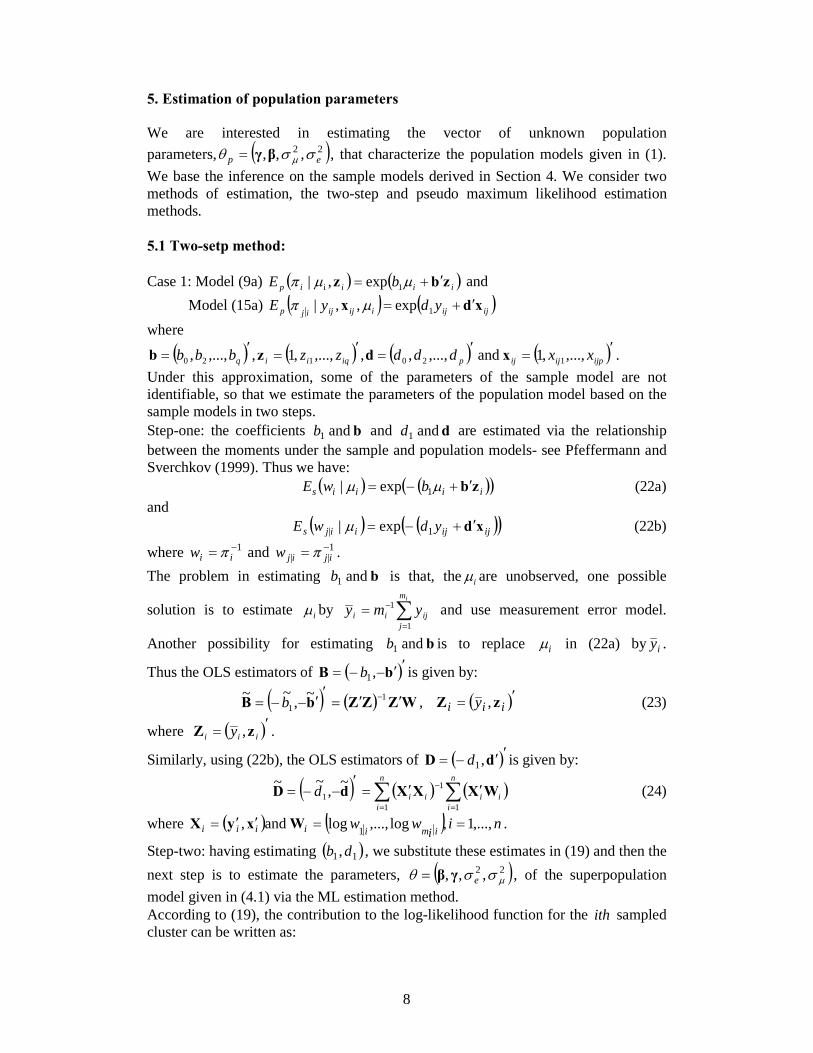
5. Estimation of population parameters We are interested in estimating the vector of unknown population parameters, ( )22 ,,, ep σσθ

µβγ= , that characterize the population models given in (1).

We base the inference on the sample models derived in Section 4. We consider two methods of estimation, the two-step and pseudo maximum likelihood estimation methods. 5.1 Two-setp method: Case 1: Model (9a) ( ) ( )iiiip bE zbz ′+= µµπ 1i exp,| and Model (15a) ( ) ( )ijijiijijijp ydyE xdx ′+=

1exp,,| µπ where

( ) ( ) ( ) ( )′=′

=′

=′

= ijpijijpiqiiq xxdddzzbbb ,...,,1 and ,...,,,,...,,1,,...,, 120120 xdzb . Under this approximation, some of the parameters of the sample model are not identifiable, so that we estimate the parameters of the population model based on the sample models in two steps. Step-one: the coefficients b and 1b and d and 1d are estimated via the relationship between the moments under the sample and population models- see Pfeffermann and Sverchkov (1999). Thus we have:

( ) ( )( )iiiis bwE zb′+−= µµ 1exp| (22a) and

( ) ( )( )ijijiijs ydwE xd′+−= 1| exp| µ (22b)

where 1−= iiw π and 1

||−

= ijijw π . The problem in estimating b and 1b is that, the iµ are unobserved, one possible

solution is to estimate iµ by ∑=

−

=

im

jijii ymy

1

1 and use measurement error model.

Another possibility for estimating b and 1b is to replace iµ in (22a) by iy .

Thus the OLS estimators of ( )′′−−= bB ,1b is given by:

( ) ( ) WZZZbB ′′=′′−−=

−11

~,~~ b , ( )′= iii y zZ , (23)

where ( )′= iii y zZ , .

Similarly, using (22b), the OLS estimators of ( )′′−= dD ,1d is given by:

( ) ( ) ( )∑∑==

−

′′=′

−−=

n

iii

n

iiid

11

11

~,~~ WXXXdD (24)

where ( ) ( ) niww imiiiii i,...,1,log,...,log and, 1 ==′′=

WxyX .

Step-two: having estimating ( )11,db , we substitute these estimates in (19) and then the next step is to estimate the parameters, ( )22 ,,,

µσσθ eγβ= , of the superpopulation

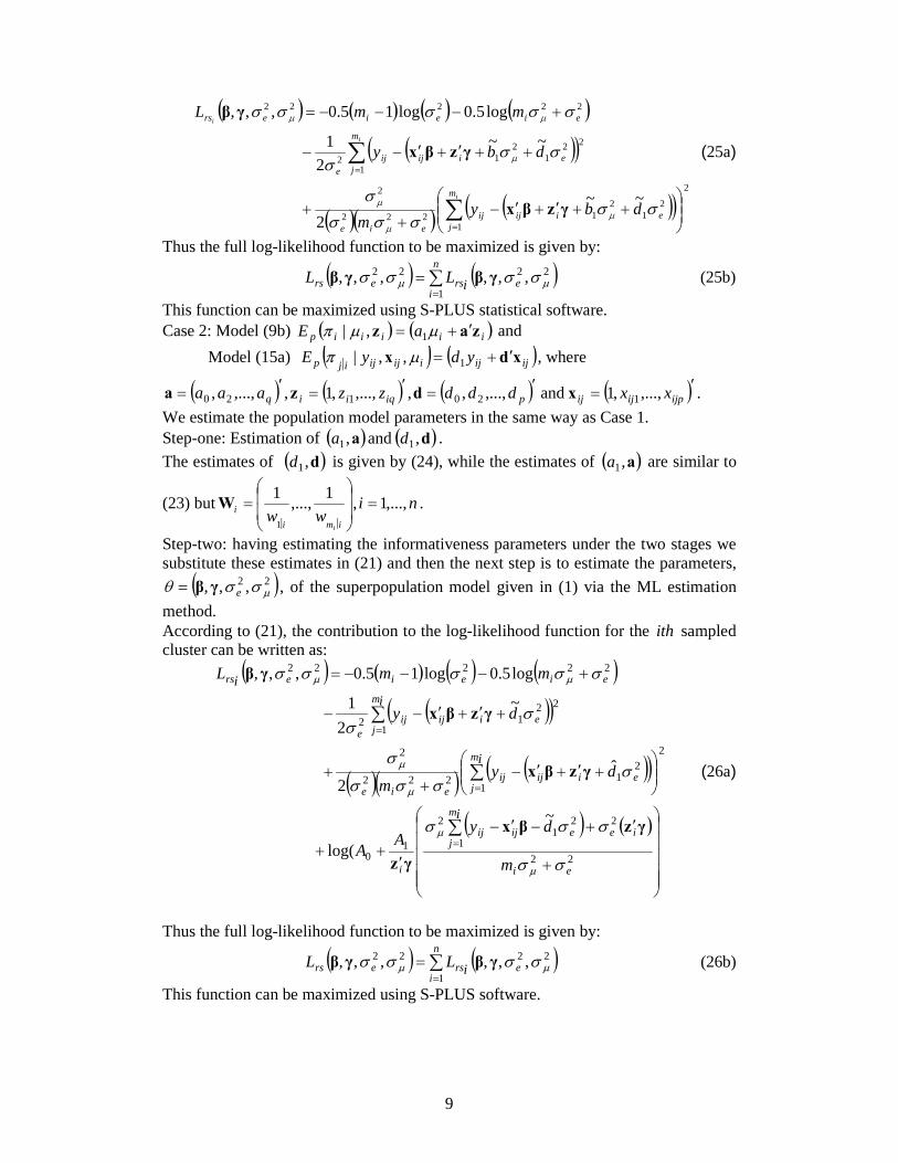
model given in (4.1) via the ML estimation method. According to (19), the contribution to the log-likelihood function for the ith sampled cluster can be written as:

9

( ) ( ) ( ) ( )

( )( )

( )( )( )( )

2

1

21

21222

2

1

221

212

22222

~~2

~~2

1

log5.0log15.0,,,

++′+′−

++

++′+′−−

+−−−=

∑

∑

=

=

i

i

i

m

jeiijij

eie

m

jeiijij

e

eieiers

dbym

dby

mmL

σσ

σσσ

σ

σσ

σ

σσσσσ

µ

µ

µ

µ

µµ

γzβx

γzβx

γβ

(25a)

Thus the full log-likelihood function to be maximized is given by:

( ) ( )∑=

=

n

iersers iLL

1

2222 ,,,,,,µµ

σσσσ γβγβ (25b)

This function can be maximized using S-PLUS statistical software. Case 2: Model (9b) ( ) ( )iiiiip aE zaz ′+= µµπ 1,| and Model (15a) ( ) ( )ijijiijijijp ydyE xdx ′+=

1,,| µπ , where

( ) ( ) ( ) ( )′=′

=′

=′

= ijpijijpiqiiq xxdddzzaaa ,...,,1 and ,...,,,,...,,1,,...,, 120120 xdza . We estimate the population model parameters in the same way as Case 1. Step-one: Estimation of ( ) ( )da , and , 11 da . The estimates of ( )d, 1d is given by (24), while the estimates of ( ) ,1 aa are similar to

(23) but niww imi

i

i

,...,1,1,...,1

1

=

=

W .

Step-two: having estimating the informativeness parameters under the two stages we substitute these estimates in (21) and then the next step is to estimate the parameters,

( )22 ,,,µ

σσθ eγβ= , of the superpopulation model given in (1) via the ML estimation method. According to (21), the contribution to the log-likelihood function for the ith sampled cluster can be written as:

( ) ( ) ( ) ( )

( )( )

( )( )( )( )

( ) ( )

~

log(

ˆ2

~2

1

log5.0log15.0,,,

221

221

2

10

2

1

21222

2

1

2212

22222

+

′+−′−

′++

+′+′−

++

+′+′−−

+−−−=

∑

∑

∑

=

=

=

ei

m

jieeijij

i

m

jeiijij

eie

m

jeiijij

e

eieiers

m

dyAA

dym

dy

mmL

i

i

ii

σσ

σσσ

σ

σσσ

σ

σ

σ

σσσσσ

µ

µ

µ

µ

µµ

γzβx

γz

γzβx

γzβx

γβ

(26a)

Thus the full log-likelihood function to be maximized is given by:

( ) ( )∑=

=

n

iersers iLL

1

2222 ,,,,,,µµ

σσσσ γβγβ (26b)

This function can be maximized using S-PLUS software.

10

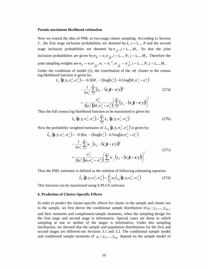
Pseudo maximum likelihood estimation Now we extend the idea of PML to two-stage cluster sampling. According to Section 2 , the first stage inclusion probabilities are denoted by Nii ,...,1, =π and the second stage inclusion probabilities are denoted by iij Mj ,...,1, =

π . So that the joint

inclusion probabilities are given by iijiij MjNi ,...,1;,...,1, === πππ . Therefore the

joint sampling weights are iijiiiij MjNiwwwwwijij

,...,1;,...,1,,, 11=====

−

−

ππ .

Under the conditions of model (1), the contribution of the ith cluster to the census log-likelihood function is given by:

( ) ( ) ( ) ( )

( )( )

( )( )( )( )

2

1222

2

1

22

22222

2

21

log5.0log15.0,,,

′+′−

++

′+′−−

+−−−=

∑

∑

=

=

i

i

i

M

jiijij

eie

M

jiijij

e

eieieC

yM

y

MML

γzβx

γzβx

γβ

σσσ

σ

σ

σσσσσ

µ

µ

µµ

(27a)

Thus the full census log-likelihood function to be maximized is given by:

( ) ( )∑=

=

N

ieCeC i

LL1

2222 ,,,,,,µµ

σσσσ γβγβ (27b)

Now the probability weighted estimator of ( )22 ,,,µ

σσ eCiL γβ is given by:

( ) ( ) ( ) ( )

( )( )

( )( )( )( )

2

21

log5.0log15.0,,,ˆ

2

1222

2

1

22

22222

′+′−

++

′+′−−

+−−−=

∑

∑

=

=

i

ij

i

ij

i

m

jiijij

eie

m

jiijij

e

eieieC

ywm

yw

mmL

γzβx

γzβx

γβ

σσσ

σ

σ

σσσσσ

µ

µ

µµ

(27c)

Thus the PML estimator is defined as the solution of following estimating equation:

( ) ( )∑=

=

n

ieCieC iLwL

1

2222 ,,,ˆ,,,ˆµµ

σσσσ γβγβ (27d)

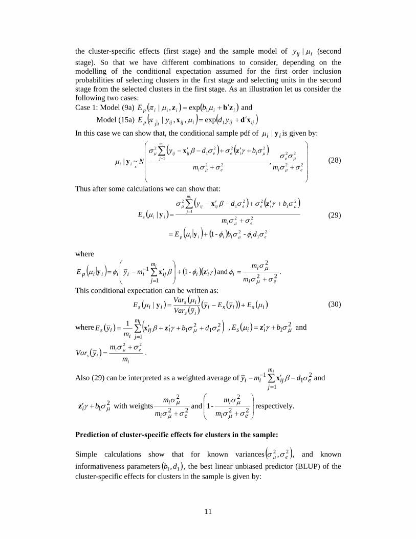
This function can be maximized using S-PLUS software. 6. Prediction of Cluster-Specific Effects In order to predict the cluster-specific effects for cluster in the sample and cluster not in the sample, we first derive the conditional sample distribution of iimii yy ,...,| 1µ , and their moments and complement-sample moments, when the sampling design for the first stage and second stage is informative. Special cases are those in which sampling at one or neither of the stages is informative. Under this sampling mechanism, we showed that the sample and population distributions for the first and second stages are different-see Sections 3.1 and 3.2. The conditional sample model and conditional sample moments of iimii yy ,...,| 1µ depend on the sample model of

11

the cluster-specific effects (first stage) and the sample model of iijy µ| (second stage). So that we have different combinations to consider, depending on the modelling of the conditional expectation assumed for the first order inclusion probabilities of selecting clusters in the first stage and selecting units in the second stage from the selected clusters in the first stage. As an illustration let us consider the following two cases: Case 1: Model (9a) ( ) ( )iiiip bE zbz ′+= µµπ 1i exp,| and Model (15a) ( ) ( )ijijiijijijp ydyE xdx ′+=

1exp,,| µπ

In this case we can show that, the conditional sample pdf of ii y|µ is given by:

( ) ( ) ,~| 22

22

221

21

221

2

++

+′+−′−∑=

ei

e

ei

m

jieeijij

sii mm

bdyN

i

σσ

σσ

σσ

σγσσβσ

µµ

µ

µ

µµzx

y (28)

Thus after some calculations we can show that:

( )

( ) ( )

( ) ( ) --1

|

21

21

221

21

221

2

eiiiip

ei

m

jieeijij

iis

dbE

m

bdyE

i

σφσφµ

σσ

σγσσβσ

µ

µ

µ

µµ

+=

+

+′+−′−

=∑=

y

zxy (29)

where

( ) ( )( ) . and -122

2

1

1

ei

iiii

m

jijiiiiip

m

mmyE

i

σσ

σφγφβφµ

µ

µ

+=′+

′−= ∑

=

− zxy

This conditional expectation can be written as:

( )( )( )

( )( ) ( ) | isisiis

isiis EyEy

yVarVar

E µµ

µ +−=y (30)

where ( ) ( ) 1

1

21

21∑

=

++′+′=

im

jeiij

iis db

myE σσγβ µzx , ( ) 2

1 µσγµ bE iis +′= z and

( )i

eiis m

myVar

22σσ

µ+

= .

Also (29) can be interpreted as a weighted average of ∑=

−

−′−

im

jeijii dmy

1

21

1σβx and

21 µσγ bi +′z with weights

++ 22

2

22

2 -1 and

ei

i

ei

i

m

m

m

m

σσ

σ

σσ

σ

µ

µ

µ

µ respectively.

Prediction of cluster-specific effects for clusters in the sample: Simple calculations show that for known variances ( )22 , eσσ

µ, and known

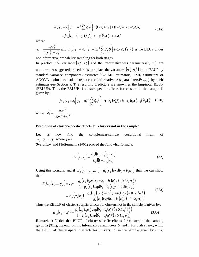
informativeness parameters ( )11,db , the best linear unbiased predictor (BLUP) of the cluster-specific effects for clusters in the sample is given by:

12

( )( ) ( )

( )( ) ( ) --1ˆ-1 ˆ

,--1ˆ-1ˆˆ

21

21,

21

21

1

1,

eiiiisui

eiiii

m

jijiiissi

db

dbmyi

σφσφγφµ

σφσφγφβφµ

µ

µ

+′+=

+′+

′−= ∑

=

−

zy

zxy (31a)

where

22

2

ei

ii m

mσσ

σφ

µ

µ

+

= and sui y,µ̂ = ( )( )γφβφ ˆ-1ˆ1

1ii

m

jijiii

imy zx ′+

′− ∑

=

− is the BLUP under

noninformative probability sampling for both stages. In practice, the variances ( )22 , eσσ

µ and the informativeness parameters ( )11,db are

unknown. A suggested procedure is to replace the variances ( )22 , eσσµ

in the BLUP by standard variance components estimates like ML estimators, PML estimators or ANOVA estimators and to replace the informativeness parameters ( )11,db by their estimates-see Section 5. The resulting predictors are known as the Empirical BLUP (EBLUP). Thus the EBLUP of cluster-specific effects for clusters in the sample is given by:

( )( ) ( ) 21

21

1

1, ˆ~ˆ-~ˆ-1ˆˆ-1ˆˆˆ eiiii

m

jijiiissi dbmy

iσφσφγφβφµ µ+′+

′−= ∑

=

− zxy (31b)

where 22

2

ˆˆ

ˆ ˆ

ei

ii m

mσσ

σφ

µ

µ

+

= .

Prediction of cluster-specific effects for clusters not in the sample: Let us now find the complement-sample conditional mean of

nj yy ,...,| 1µ where sj ∉ . Sverchkov and Pfeffermann (2001) proved the following formula:

( ) ( )( )( )( )jjp

jjjpjjc xE

xyExyE

−

−=

π

π

1

1 (32)

Using this formula, and if ( ) ( ) ( )jjejjp bbgE µµπ 10j exp,| += zz then we can show that:

( ) ( ) ( )( )( ) ( )( )

( ) ( ) ( )( )( ) ( )( )22

110

22110

21

22110

22110

21

1

5.0exp15.0exp

5.0exp15.0exp

,...,

µ

µµ

µ

µµ

σγ

σγσµ

σγ

σγσγµ

bbbgbbbbg

E

bbbgbbbbg

E

jje

jjejjp

jje

jjejnjc

+′+−

+′+−=

+′+−

+′+−′=

zzzz

z

zzzz

zyy

(33a)

Thus the EBLUP of cluster-specific effects for clusters not in the sample is given by:

( ) ( )( )

( ) ( )( )

ˆ5.0ˆ~exp~1

ˆ~5.0ˆ~~expˆ~~ˆˆ

22110

22110

21

,µ

µµ

σγ

σγσγµ

bbbgbbbbg

jje

jjejscj

+′+−

+′+−′=

zzzz

zy (33b)

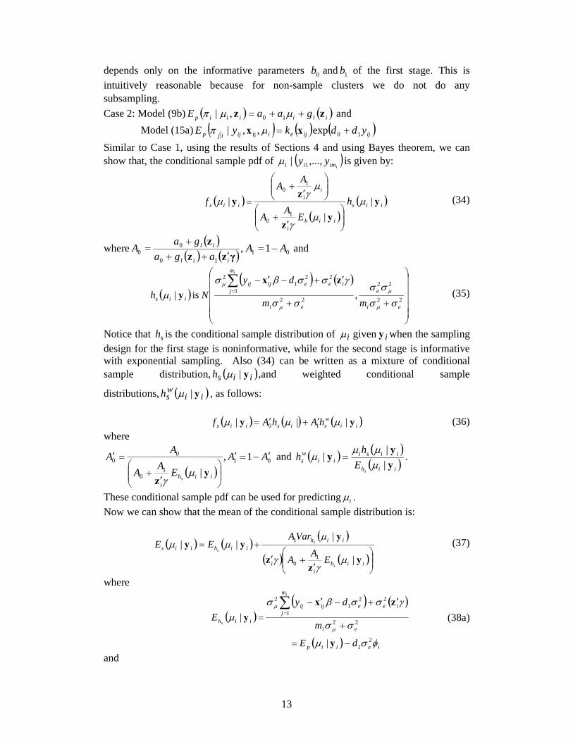
Remark 1: Notice that BLUP of cluster-specific effects for clusters in the sample, given in (31a), depends on the informative parameters 11 and db for both stages, while the BLUP of cluster-specific effects for clusters not in the sample given by (33a)

13

depends only on the informative parameters and 10 bb of the first stage. This is intuitively reasonable because for non-sample clusters we do not do any subsampling. Case 2: Model (9b) ( ) ( )iliiip gaaE zz ++= µµπ 10i ,| and Model (15a) ( ) ( ) ( )ijijeiijijp yddkyE 10ij exp,,| +=

xx µπ

Similar to Case 1, using the results of Sections 4 and using Bayes theorem, we can show that, the conditional sample pdf of ( )

iimii yy ,...,| 1µ is given by:

( )

( )

( )iis

iihi

ii

iis hE

AA

AA

f yy

z

zy |

||

10

10

µ

µγ

µγ

µ

′+

′+

= (34)

where( )

( ) ( ) 0110

00 1 , AA

agagaA

iil

il−=

′++

+=

γzzz

and

( )( ) ( )

, is | 22

22

221

221

2

++

′+−′−∑=

ei

e

ei

m

jieeijij

iis mm

dyNh

i

σσ

σσ

σσ

γσσβσ

µµ

µ

µ

µzx

y (35)

Notice that sh is the conditional sample distribution of ii ygiven µ when the sampling design for the first stage is noninformative, while for the second stage is informative with exponential sampling. Also (34) can be written as a mixture of conditional sample distribution, ( )iish y|µ ,and weighted conditional sample

distributions, ( )iiwsh y|µ , as follows:

( ) ( ) ( ) || | 10 ii

wsisiis hAhAf yy µµµ ′+′= (36)

where

( ) 1,

|01

10

00 AA

EAA

AA

iihi

s

′−=′

′+

=′

yz

µγ

and ( )( )( )iih

iisiii

ws

sE

hhyyy

||

| µ

µµµ = .

These conditional sample pdf can be used for predicting iµ . Now we can show that the mean of the conditional sample distribution is:

( ) ( )( )

( ) ( )

|

|||

10

1

′+′

+=

iihi

i

iihiihiis

s

s

s

EAA

VarAEE

yz

z

yyy

µγ

γ

µµµ (37)

where

( )

( ) ( )

( ) ieiip

ei

m

jieeijij

iih

dE

m

dyE

i

s

φσµ

σσ

γσσβσ

µµ

µ

21

221

221

2

|

|

−=

+

′+−′−

=

∑=

y

zxy (38a)

and

14

( ) ( )iipei

eiih Var

mVar

syy || 22

22

µσσ

σσµ

µ

µ

=

+

= (38b)

Notice that ( ) ( )iihiis sEE yy |=| µµ if and only if 01 =A , and this happens when

01 =a , that is, when the sampling design for the first stage is noninformative. Also ( ) ( )iipiih EE

syy |=| µµ if and only if 01 =d , that is the sampling design for the

second stage is noninformative. Under this sample conditional pdf, simple calculations show the EBLUP of cluster-specific effects for clusters in the sample is given by:

( )( )

( ) ( )

|ˆ

ˆ

~~ˆ

|ˆ~|ˆ|ˆ

10

1,

′+′

+=

iihi

i

iihiihssi

s

s

s

EAA

arVAE

yz

z

yyy

µγ

γ

µµµ (39a)

where

( )( ) ( )

221

221

2

ˆˆ

ˆˆˆ~ˆˆ|ˆ

ei

m

jieeijij

iih m

dyE

i

s σσ

γσσβσ

µµ

µ

+

′+−′−

=

∑=

zxy , ( )

22

22

ˆˆ

ˆˆ|ˆ

ei

eiih

marV

sσσ

σσ

µ

µ

µ

+

=y

( )( ) ( ) 01

10

00

~1~ and ˆ~~~

~~~ AAaga

gaA

iil

il−=

′++

+=

γzzz

.

Prediction of cluster-specific effects for clusters not in the sample: Let us now find the conditional complement-sample mean of

( )′=iimiinj yy ,..., ;,...,| 11 yyyµ where sj ∉ . Similar to Case 1, but

here: ( ) ( )( )jjljjp agaE µµπ 10j ,| ++= zz . In this case we can show that the EBLUP of cluster-specific effects for clusters not in the sample is given by:

( ) ( )( )γ

σγµ

µ

ˆ~~~1ˆ~

ˆˆ10

21

,jjl

jscj agaa

zzzy

′++−−′= (40)

Remark 1: Notice that EBLUP of cluster-specific effects for clusters in the sample, given in (39a), depends on the informative parameters 110 and , daa for both stages, while the EBLUP of cluster-specific effects for clusters not in the sample given by (40) depends only on the informative parameters and 10 aa of the first stage. This is intuitively reasonable because for non-sample clusters we do not do any subsampling. 7. Prediction of finite population total under two-stage informative cluster sampling Assume two-stage population model (1). Let

∑ ∑ ∑∑∑∑∑∑= += += == == =

++==

n

i

M

mj

N

ni

M

jijij

n

i

m

jij

N

i

M

jij

i

i

iii

yyyyT1 1 1 11 11 1

(41)

15

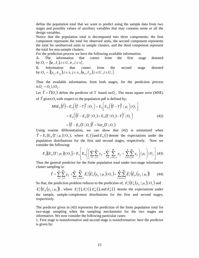
define the population total that we want to predict using the sample data from two stages and possibly values of auxiliary variables that may contains some or all the design variables. Notice that the population total is decomposed into three components: the first component represents the total for observed units, the second component represents the total for unobserved units in sample clusters, and the third component represent the total for non-sample clusters. For the prediction process we have the following available information: A. The information that comes from the first stage denoted by: ( ){ }siUiIO iii ∈∈= ,,,,1 πz . B. Information that comes from the second stage denoted by: ( ) ( ){ }iijijiijij UjUiIsjsiyO ∈∈∈∈= ,,,,,,, ||2 xπ . Thus the available information, from both stages, for the prediction process is 21 OOOs s= .

Let ( )sOTT ˆˆ= define the predictor of T based on sO . The mean square error (MSE)

of sOT given ˆ with respect to the population pdf is defined by:

( ) ( ) ( )

( ) ( )( )

( )( ) ( )spsP

ssPsPP

siIIIsPP

OTVarOTET

OTOTEOTETE

OTTEEOTTETMSE

||ˆ

|||ˆ

||ˆ|ˆˆ

2

2

22

+−=

−+−=

−=

−= µ

(42)

Using routine differentiation, we can show that (42) is minimized when ( )( )sO||ˆ

iIII TEET µ= , where ( ) ( ) and ⋅⋅ III EE denote the expectations under the population distributions for the first and second stages, respectively. Now we consider the following:

( )( )[ ]

++= ∑ ∑ ∑∑∑∑

= += += == =

s1 1 1 11 1

s O||O|| i

n

i

M

mj

N

ni

M

jijij

n

i

m

jijIIIiIII

i

i

ii

yyyEETEE µµ (43)

Thus the general predictor for the finite population total under two-stage informative cluster sampling is:

( )( ) ( )( )∑ ∑ ∑∑∑∑= += += == =

++=

n

i

M

mj

N

ni

M

jiijII

cIiij

cII

sI

n

i

m

jij

i

i

ii

yEEyEEyT1 1 1 1

s1 1

|ˆˆO||ˆˆˆ µµ (44)

So that, the prediction problem reduces to the prediction of, ( )( ) O|| siµijcII

sI yEE and

( )( ) | iµijIIcI yEE , where ( ) ( ) ( ) ( ) and , , , ⋅⋅⋅⋅

sII

cII

cI

sI EEEE denote the expectations under

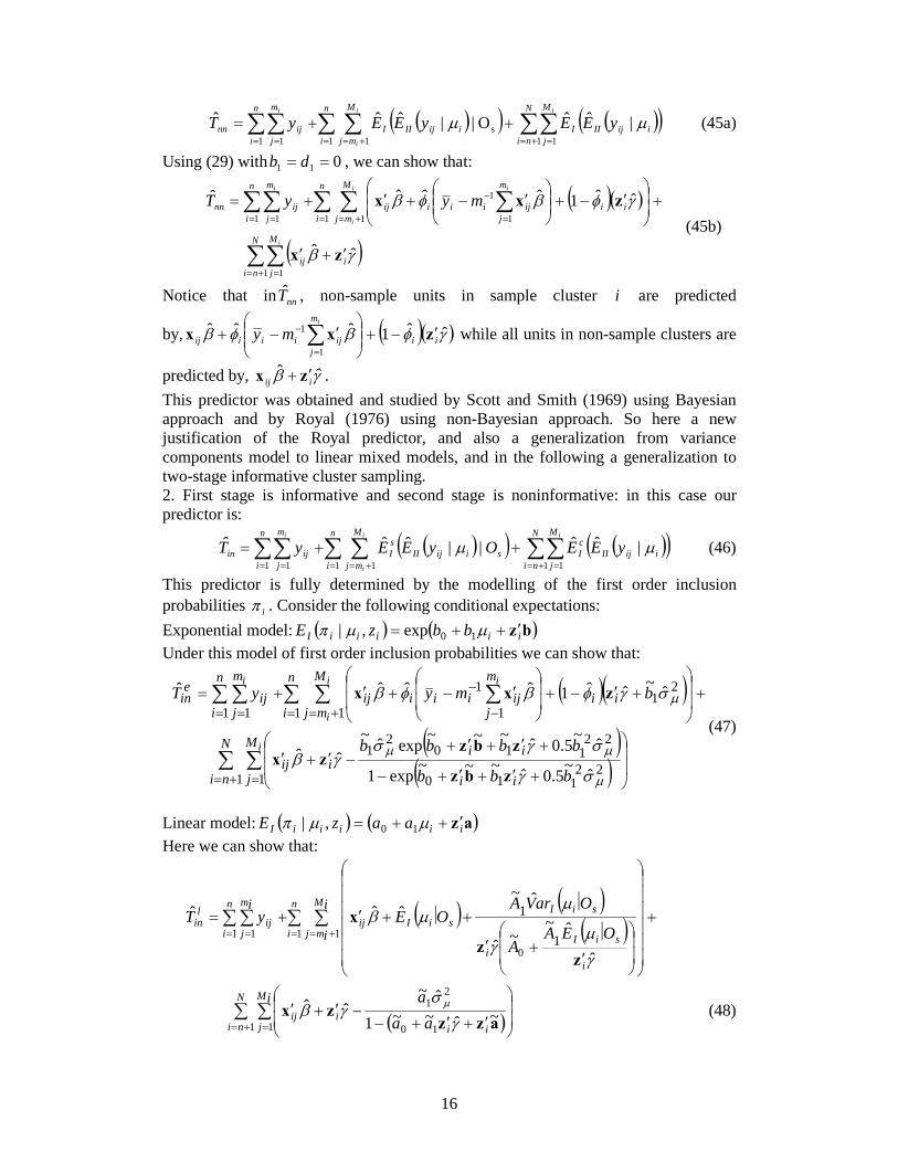
the sample, sample-complement distributions for the first and second stages, respectively. The predictor given in (43) represents the prediction of the finite population total for two-stage sampling when the sampling mechanisms for the two stages are informative. We now consider the following particular cases: 1. First stage is noninformative and second stage is noninformative: here the predictor is given by:

16

( )( ) ( )( )∑ ∑ ∑∑∑∑= += += == =

++=

n

i

M

mj

N

ni

M

jiijIIIiijIII

n

i

m

jijnn

i

i

ii

yEEyEEyT1 1 1 1

s1 1

|ˆˆO||ˆˆˆ µµ (45a)

Using (29) with 011 == db , we can show that:

( )( )

( )∑∑

∑ ∑ ∑∑∑

+= =

= += =

−

= =

′+′

+

′−+

′−+′+=

N

ni

M

jiij

n

i

M

mjii

m

jijiiiij

n

i

m

jijnn

i

i

i

ii

myyT

1 1

1 1 1

1

1 1

ˆˆ

ˆˆ1ˆˆˆ ˆ

γβ

γφβφβ

zx

zxx (45b)

Notice that in nnT̂ , non-sample units in sample cluster i are predicted

by, ( )( )γφβφβ ˆˆ1ˆˆˆ1

1ii

m

jijiiiij

i

my zxx ′−+

′−+ ∑

=

− while all units in non-sample clusters are

predicted by, γβ ˆˆiij zx ′+ .

This predictor was obtained and studied by Scott and Smith (1969) using Bayesian approach and by Royal (1976) using non-Bayesian approach. So here a new justification of the Royal predictor, and also a generalization from variance components model to linear mixed models, and in the following a generalization to two-stage informative cluster sampling. 2. First stage is informative and second stage is noninformative: in this case our predictor is:

( )( ) ( )( )∑ ∑ ∑∑∑∑= += += == =

++=

n

i

M

mj

N

ni

M

jiijII

cIsiijII

sI

n

i

m

jijin

i

i

ii

yEEOyEEyT1 1 1 11 1

|ˆˆ||ˆˆ ˆ µµ (46)

This predictor is fully determined by the modelling of the first order inclusion probabilities iπ . Consider the following conditional expectations: Exponential model: ( ) ( )bz iiiiiI bbzE ′++= µµπ 10exp,| Under this model of first order inclusion probabilities we can show that:

( )( )

( )( )

ˆ~5.0ˆ~~~exp1

ˆ~5.0ˆ~~~expˆ~ˆˆ

ˆ~ˆˆ1ˆˆˆˆ

1 122

110

22110

21

1 1

21

1

1

1 1

∑ ∑

∑ ∑ ∑∑∑

+= =

= += −

−

= =

+′+′+−

+′+′+−′+′

+

+′−+

′−+′+=

N

ni

M

j ii

iiiij

n

i

M

mjii

m

jijiiiij

n

i

m

jij

ein

i

i

i

ii

bbb

bbbb

bmyyT

µ

µµ

µ

σγ

σγσγβ

σγφβφβ

zbz

zbzzx

zxx

(47)

Linear model: ( ) ( ) ,| 10 az iiiiiI aazE ′++= µµπ Here we can show that:

( ) ( )( )

( )

~ˆ~~1ˆ~

ˆˆ

ˆ

ˆ~~ˆ

ˆ~ˆˆˆ

1 1 10

21

1 1

0

1 1 1

1

∑ ∑

∑ ∑∑∑

+= =

= +== =

′+′+−−′+′

+

′

+′

++′+=

N

ni

M

j iiiij

n

i

M

mj

i

siIi

siIsiIij

n

i

m

jij

lin

i

i

i

i

aaa

OEAA

OarVAOEyT

azzzx

zz

x

γ

σγβ

γ

µγ

µµβ

µ (48)

17

where

( )siI OE µ = ( )( )γφβφ ii

m

jijiii

i

my zx ′−+

′− ∑

=

− 11

1 , ( )i

ei

ei

esiI mm

OVar2

22

22σφ

σσ

σσµ

µ

µ =+

=

( )( )

( )γγ

γ ii

i

ii

i

aaa

Aaa

aA

zazz

zazaz

′+′+

′=

′+′+

′+=

10

11

10

00 and .

Other cases: first stage noninformative and second stage informative and first and second stages informative can be treated in the same way but in these cases predictors have no closed forms so Taylor approximation or Monte Carlo simulation are adopted. 8. Prediction of finite population totals for sampled and non-sampled clusters In Section 8 we obtained predictors of the finite population total. But in some applications like small area estimation we are interested in predicting the small area totals for sampled and non-sampled small areas. Assume two-stage population model (5.1). Let

∑=

=

iM

jiji yT

1 (49)

define the population total for cluster Ui∈ that we want to predict using the sample data from two stages and possibly values of auxiliary variables that may contains some or all the design variables. Prediction of cluster totals for clusters in the sample: In order to do that, let us decompose iT into two components: the first component represents the total for observed units, and the second component represents the total for unobserved units in sample clusters that is:

∑∑∑∑∑∉∈+===

+=+==

ii

i

i

ii

sjij

sjij

M

mjij

m

jij

M

jiji yyyyyT

111 (50)

Let ( )si OT̂ denotes the predictor of iT based on sO . So as in Section 8, the mean

square error with respect to the population model of iT̂ is minimised when

( )( )siiIIIi OTEET ||ˆ µ= . Thus we have:

( )( )[ ] ( )( )∑ ∑= +=

+=

i i

i

m

j

M

mjsiijIIIijsiiIII OyEEyOTEE

1 1|||| µµ (51)

Thus the general predictor for the finite cluster total under two-stage informative cluster sampling is:

( )( )[ ] ( )( )∑ ∑= +=

+==

i i

i

m

j

M

mjsiij

cII

sIijsiiIIIi OyEEyOTEET

1 1||ˆˆ||ˆ µµ (52)

So that, the prediction problem reduces to the prediction of, ( )( ) || i sij

cII

sI OyEE µ under a specified sampling design.

1. First stage is noninformative and second stage is noninformative: here the predictor is given by:

18

( ) ( )( )∑ ∑ ∑= += =

−

′−+

′−+′+=∈

i i

i

im

j

M

mjii

m

jijiiiijijnn myysiT

1 1 1

1 ˆˆ1ˆˆˆˆ γφβφβ zxx (53)

Notice that in ( )siTnn ∈ˆ , non-sample units in sample cluster i are predicted by,

( )( )γφβφβ ˆˆ1ˆˆˆ1

1ii

m

jijiiiij

i

my zxx ′−+

′−+ ∑

=

− .

2. First stage is informative and second stage is noninformative: in this case if the conditional expectation of the first order inclusion probabilities is exponential, then

( ) ( )( )∑ ∑ ∑= += −

−

+′−+

′−+′+=∈

i i

i

im

j

M

mjii

m

jijiiiijij

ein bmyysiT

1 1

21

1

1 ˆ~ˆˆ1ˆˆˆˆµ

σγφβφβ zxx (54)

Now if the conditional expectation of the first order inclusion probabilities is linear, then we have:

( ) ( ) ( )( )

∑ ∑= +=

′

+′

++′+=∈

i i

i

m

j

M

mj

i

siIi

siIsiIijij

lin

OEAA

OarVAOEysiT

1 1

0 ˆ

ˆ~~ˆ

ˆ~ˆˆˆ

1

1

γ

µγ

µµβ

zz

x (55)

where

( )siI OE µ = ( )( )γφβφ ii

m

jijiii

i

my zx ′−+

′− ∑

=

− 11

1 , ( )i

ei

ei

esiI mm

OVar2

22

22σφ

σσ

σσµ

µ

µ =+

=

and

( )( )

( )γγ

γ ii

i

ii

i

aaa

Aaa

aA

zazz

zazaz

′+′+

′=

′+′+

′+=

10

11

10

00 and .

Similar procedures for other cases. Prediction of cluster totals for clusters not in the sample Here the decomposition of the finite cluster total into observed and unobserved units does not help, because for si∉ we do not observe any unit. Thus similar to the previous section, the predictor of the non-sample finite cluster total is:

( ) ( )( )[ ] ( )( )∑=

==∉

iM

jiijII

cIiiIIIi yEETEEsiT

1|ˆˆ|ˆ µµ (56)

Let us study this predictor under different sampling design for the first stage, and since we do not observe any unit in the second stage therefore no sampling design is considered of the second stage. 1. First stage noninformative: Under this sampling design our predictor is given by:

( ) ( )∑=

′+′=∉

iM

jiijnn siT

1

ˆˆˆ γβ zx (57)

2. First stage informative: Under the exponential model we have the following predictor:

( )( )( )( )( )∑

=

+′+′+−

+′+′+−′+′=∉

iM

j ii

iiiji

ein bbb

bbbbsiT

122

110

22110

21

ˆ~5.0ˆ~~~exp1

ˆ~5.0ˆ~~~expˆ~ˆˆˆ

µ

µµ

σγ

σγσβγ

zbz

zbzxz (58)

Under the linear model, the predictor is given by:

19

( )( )( )

∑=

′+′+−−′+′=∉

iM

j iiiji

lin aa

asiT

1 10

21

ˆ~~~1ˆ~

ˆˆˆγ

σβγ

µ

zazxz (59)

References Amin, M. (2001). Estimation of the parameters of a two-stage model under informative sampling, based on the sampling distribution, Master thesis, Department of Statistics, Hebrew University of Jerusalem. Chambers, R. and Skinner, C. (2003).Analysis of Survey Data. New York: John Wiley. Cochran, W.G. (1977). Sampling Techniques (3rd Ed.). New York: John Wiley. Lohr, S.L. (1999). Sampling: design and analysis, London: Brooks/Cole. Pfeffermann, D., Krieger, A.M, and Rinott, Y. (1998). Parametric distributions of complex survey data under informative probability sampling. Statistica Sinica 8: 1087-1114. Pfeffermann, D., Moura, F. A. S. and Nascimaneto-Silva, P.L. (2001). Multilevel modeling under informative sampling. Proceedings of the Invited Paper Sessions Organized by the International Association of Survey Statisticians (IASS) for the 53rd session of the International Statistical Institute, pp. 505-532. Pfeffermann, D., Skinner, C.J., Goldstein, H., Holmes, D.J, and Rasbash, J. (1998). Weighting for unequal selection probabilities in multilevel models (with discussion). Journal of the Royal Statistical Society, Series B, 60: 23-40. Pfeffermann, D. and Sverchkov, M. (1999). Parametric and semi-parametric estimation of regression models fitted to survey data. Sankhya, 61, Ser. B, Pt. 1: 166-186Royall, R.M. (1976). The linear least squares prediction approach to two-stage sampling. Journal of the American Statistical Association 71: 657-664. Sarndal, C-E., Swensson, B., and Wretman, J. (1992). Model assisted survey sampling, New York: Springer. Skinner, C.J. (1994). Sample models and weights. American Statistical Association Proceeding of the Section on Survey Research Methods, 133-142. Statistical Sciences, (1990). S-Plus Reference Manual, Seattle: Statistical Sciences. Sverchkov, M. and Pfeffermann, D. (2001). Prediction of finite population totals under informative sampling utilizing the sample distribution. American Statistical Association Proceedings of the Section on Survey Research Methods, 41-46.

20