Embed Size (px)
Citation preview
HAL Id: tel-00708397https://tel.archives-ouvertes.fr/tel-00708397
Submitted on 15 Jun 2012
HAL is a multi-disciplinary open accessarchive for the deposit and dissemination of sci-entific research documents, whether they are pub-lished or not. The documents may come fromteaching and research institutions in France orabroad, or from public or private research centers.
L’archive ouverte pluridisciplinaire HAL, estdestinée au dépôt et à la diffusion de documentsscientifiques de niveau recherche, publiés ou non,émanant des établissements d’enseignement et derecherche français ou étrangers, des laboratoirespublics ou privés.
Two studies in risk management: portfolio insuranceunder risk measure constraint and quadratic hedge for
jump processes.Carmine de Franco
To cite this version:Carmine de Franco. Two studies in risk management: portfolio insurance under risk measure constraintand quadratic hedge for jump processes.. Probability [math.PR]. Université Paris-Diderot - Paris VII,2012. English. tel-00708397
UNIVERSITE PARIS 7 - Denis DiderotUFR de MATHEMATIQUES
Ecole Doctorale de Sciences Mathematiques de Paris Centre
These presentee pour obtenir le titre de
DOCTEUR DE L’UNIVERSITE PARIS DIDEROT
Specialite: mathematiques appliquees
presentee par
Carmine DE FRANCO
Deux etudes en gestion de risque: assurance deportefeuille avec contrainte en risque et
couverture quadratique dans les modeles a sauts
Two studies in risk management: portfolio insurance under riskmeasure constraint and quadratic hedge for jump processes.
These dirigee par
Prof. Peter TANKOVSoutenue publiquement le 29 Juin 2012 devant le jury compose de:
ACHDOU Yves, Professeur, Universite Paris Diderot
BOUCHARD Bruno, Professeur, Universite Paris Dauphine
LAMBERTON Damien, Professeur, Universite de Marne-la-Vallee
PHAM Huyen, Professeur, Universite Paris Diderot
SULEM Agnes, Directeur de recherche, INRIA
WARIN Xavier, Departement R&D, EDF France
au vu des rapports de:
KALLSEN Jan, Professeur, Christian-Albrechts Universitat zu Kiel
LAMBERTON Damien, Professeur, Universite de Marne-la-Vallee


A mia madre Iride,mio padre Francesco,
a Caterina e Vincenzo

Remerciements
Je tiens a remercier mon directeur de these Peter Tankov, qui m’a fortement soutenu pen-dant ces annees de recherche et avec lequel j’ai passe de tres beaux moments intenses etagreables. J’ai pu profiter de toute son experience en mathematiques financieres et des nom-breuses discussions qu’on a eu le long de mon doctorat. Pour cela je lui serai eternellementreconnaissant.
Je tiens a exprimer ma gratitude a Jan Kallsen et Damien Lamberton pour avoir accepte derapporter cette these, et a tous les membres du jury. Je remercie aussi l’Universite Paris VIIet le Laboratoire de Probabilites et Modeles Aleatoires qui ont ete des environnements detravail tres serieux. En particulier, je veux exprimer toute ma reconnaissance a Prof. YvesAchdou pour l’aide precieuse qu’il m’a fourni, en premier lieu lorsque j’etais un etudiantErasmus, puis comme professeur a Paris VII et enfin comme son assistant-charge de travauxdiriges. Ensuite aux Prof. Laure Elie et Prof. Huyen Pham pour leurs cours de finance etoptimisation stochastique que j’ai eu la chance de suivre pendant mon Master. Je remer-cie aussi le Centre de Mathematiques Appliquees de l’Ecole Polytechnique et son groupede travail auquel j’ai partecipe et a qui ma formation doit beaucoup. A Xavier Warin etNadia Oudjane du departement R&D de EDF va toute ma reconnaissance pour la precieusecollaboration a ce travail.
Si aujourd’hui j’ai pu completer ma formation en mathematiques, je le dois aussi aux ex-cellents cours que j’ai pu suivre a l’ Universita degli studi di Roma II -Tor Vergata, etune pensee particuliere va aux Prof. Claudio D’Antoni, Roberto Longo, Mauro Nacinovichet Stefano Trapani. J’exprime ma gratitude la plus sincere aux Prof. Paolo Baldi et Prof.Domenico Marinucci pour avoir su motiver ma passion pour le probabilites. Affectueusementma gratitude va aux Prof. Carmine Armentano et Prof. Francesco Romano de Mormanno.
Nombreux sont ceux qui, pendant ces annees, ont toujours manifeste de l’interet pour montravail. En particulier, pour les tres beaux moments passes ensemble et son support infatiga-ble, toute ma reconnaissance va a Germain Griette. Egalement a Emmanuel et Jean-BaptisteMeffre, Amber Leesa French, Claire Jarry, Jean-Marc et Stephane Boulais, Cyprien Larrouy,Marc Viader, Bruno Ludwig, Caroline Remy, Angeliki Kordoni, Sophie Albert, Eric Vignat,Sarah Orford, Sarah Louise Porter, Neil Hancox, John Gareth Wyn Williams, Roberto Ar-cone et Liam D. Gray. Pour leur amitie depuis toujours je remercie Luigi Bloise, PierluigiPerrone, Antonio Oliva et Gianni Regina.
Au Maestro Jorge De Leon, selon lequel les Mathematiques et l’Opera sont deux faces d’unememe piece, va toute mon admiration et ma gratitude pour l’experience qu’il a partage avecmoi.
A mamma, papa, fratima e sorma, ca m’anu duvutu suppurta pi tuttu stu tempu, tra iute,vinute e spirciate. ”...N’dra vita unu adda sapı mania la pinna e la zappa...” dicia quaccunuca di nummari angunu picchi ni capiscia. P’a zappa c’e sempri tempu e terri ierse certunon ti mancanu..a pinna po jessi ca mo m’ajjiu m’barata a la mania.
Paris , 29 Juin 2012 Carmine DE FRANCO

Resume
Dans cette these, je me suis interesse a deux aspects de la gestion de porte-feuille : la maximisation de l’utilite d’un portefeuille financier lorsque on imposeune contrainte sur l’exposition au risque, et la couverture quadratique en marcheincomplet.
Part I. Dans la premiere partie, j’etudie un probleme d’assurance de portefeuilledu point de vue du manager d’un fond d’investissement, qui veut structurer unproduit financier pour les investisseurs du fond avec une garantie sur la valeur duportefeuille a la maturite. Si, a la maturite, la valeur du portefeuille est au dessousd’un seuil fixe, l’investisseur sera rembourse a la hauteur de ce seuil par une troisiemepartie, qui joue le role d’assureur du fond (on peut imaginer que le fond appartienta une banque et que donc c’est la banque elle meme qui joue le role d’assureur). Enechange de cette assurance, la troisieme partie impose une contrainte sur l’expositionau risque que le manager du fond peut tolerer, mesure avec une mesure de risquemonetaire convexe. Je donne la solution complete de ce probleme de maximisationnon convexe en marche complet et je prouve que le choix de la mesure de risqueest un point crucial pour avoir existence d’un portefeuille optimal. J’applique doncmes resultats lorsque on utilise la mesure de risque entropique (pour laquelle leportefeuille optimal existe toujours), les mesures de risque spectrales (pour lesquellesle portefeuille optimal peut ne pas exister dans certains cas) et la G-divergence.Mots-cles : Assurance de portefeuille ; maximisation d’utilite ; mesure de risqueconvexe ; VaR, CVaR et mesure de risque spectrale ; entropie et G-divergence.
Part II. Dans la deuxieme partie, je m’interesse au probleme de couverture qua-dratique en marche incomplet. J’assume que le marche est decrit par un processusMarkovien tridimensionnel avec sauts. La premiere variable d’etat decrit l’actif fi-nancier, echangeable sur le marche, qui sert comme instrument de couverture ; ladeuxieme variable d’etat modelise un actif financier que intervient dans la dyna-mique de l’instrument de couverture mais qui n’est pas echangeable sur le marche :il peut donc etre vu comme un facteur de volatilite de l’instrument de couverture,ou comme un actif financier que l’on ne peut pas acheter (pour de raisons legalespar exemple) ; la troisieme et derniere variable d’etat represente une source externede risque qui affecte l’option europeenne qu’on veut couvrir, et qui, elle aussi, n’estpas echangeable sur le marche. Pour resoudre le probleme j’utilise l’approche de laprogrammation dynamique, qui me permet d’ecrire l’equation de Hamilton-Jacobi-Bellman associee au probleme de couverture quadratique, qui est non locale en nonlineaire. Je prouve que la fonction valeur associee au probleme de couverture quadra-
1
tique peut etre caracterisee par un systeme de trois equations integro-differentiellesaux derivees partielles, dont l’une est semilineaire et ne depends pas du choix del’option a couvrir, et les deux autres sont simplement lineaires , et que ce systemea une unique solution reguliere dans un espace de Holder approprie, qui me permetdonc de caracteriser la strategie de couverture optimale . Ce resultat est demontrelorsque le processus est non degenere (c’est a dire que la composante Brownienneest strictement elliptique) et lorsque le processus est a sauts purs. Je conclus avecune application de mes resultats dans le cadre du marche de l’electricite.Mots-cles : Couverture quadratique ; modele a sauts ; programmation dynamique ;equation de Hamilton-Jacobi-Bellman ; equations aux derivees partielles integro-differentielles ; espaces de Holder ; processus de Levy ; marche de l’electricite.
Abstract
In this thesis I’m interested in two aspects of portfolio management: the port-folio insurance under a risk measure constraint and quadratic hedge in incompletemarkets.
Part I. I study the problem of portfolio insurance from the point of view of a fundmanager, who guarantees to the investor that the portfolio value at maturity will beabove a fixed threshold. If, at maturity, the portfolio value is below the guaranteedlevel, a third party will refund the investor up to the guarantee. In exchange forthis protection, for which the investor pays a given fee, the third party imposes alimit on the risk exposure of the fund manager, in the form of a convex monetaryrisk measure. The fund manager therefore tries to maximize the investor’s utilityfunction subject to the risk measure constraint. I give a full solution to this non-convex optimization problem in the complete market setting and show in particularthat the choice of the risk measure is crucial for the optimal portfolio to exist.An interesting outcome is that the fund manager’s maximization problem may notadmit an optimal solution for all convex risk measures, which means that not allconvex risk measures may be used to limit fund’s exposure in this way. I provideconditions for the existence of the solution. Explicit results are provided for theentropic risk measure (for which the optimal portfolio always exists), for the classof spectral risk measures (for which the optimal portfolio may fail to exist in somecases) and for the G-divergence.Key words: Portfolio Insurance; utility maximization; convex risk measure; VaR,CVaR and spectral risk measure; entropy and G-divergence.
Part II. In the second part I study the problem of quadratic hedge in incompletemarkets. I work with a three-dimensional Markov jump process: the first compo-
2
nent is the state variable representing the hedging instrument traded in the market,the second component models a risk factor which ”perturbs” the dynamics of thehedging instrument and is not traded in the market (as a volatility factor for ex-ample in stochastic volatility models); the third one is another source of risk whichaffects the option’s payoff at maturity and is also not traded in the market. Theproblem can be seen then as a constrained quadratic hedge problem. I privilege herethe dynamic programming approach which allows me to obtain the HJB equationrelated to the value function. This equation is semi linear and non local due thepresence of jumps. The main result of this thesis is that this value function, as afunction of the initial wealth, is a second order polynomial whose coefficients arecharacterized as the unique smooth solutions of a triplet of PIDEs, the first of whichis semi linear and does not depend on the particular choice of option one wants tohedge, the other two being simply linear. This result is stated when the Markovprocess is assumed to be a non-generate jump-diffusion and when it is a pure jumpprocess. I finally apply my theoretical results to an example of quadratic hedge inthe context of electricity markets.Key words: Quadratic Hedge; jump processes; dynamic programming; Hamilton-Jacobi-Bellman equations; partial integro-differential equations; Levy processes;Holder spaces; electricity markets.

Contents
1 Introduction (French version) 11
2 Introduction 25
I Portfolio Insurance under risk measure constraint 29
3 An overview on Risk measures 31
3.1 Practical needs of the risk measures: empirical evidence . . . . . . . 31
3.2 Law invariant risk measures . . . . . . . . . . . . . . . . . . . . . . . 32
3.2.1 Definition and main properties . . . . . . . . . . . . . . . . . 32
3.2.2 Representation of convex risk measures . . . . . . . . . . . . 33
3.3 VaR, CVaR and spectral risk measures . . . . . . . . . . . . . . . . 35
3.4 G-divergence and entropy . . . . . . . . . . . . . . . . . . . . . . . . 37
3.5 Risk Measures on Lp-spaces . . . . . . . . . . . . . . . . . . . . . . 38
4 Portfolio Insurance 39
4.1 The Problem . . . . . . . . . . . . . . . . . . . . . . . . . . . . . . . 40
4.2 The decoupling and the solution . . . . . . . . . . . . . . . . . . . . 42
4.3 The fee . . . . . . . . . . . . . . . . . . . . . . . . . . . . . . . . . . 50
4.4 Explicit result: the Entropic risk measure . . . . . . . . . . . . . . . 51
4.4.1 The result . . . . . . . . . . . . . . . . . . . . . . . . . . . . . 51
4.4.2 Numerical example . . . . . . . . . . . . . . . . . . . . . . . . 53
4.5 Explicit result: the spectral risk measure . . . . . . . . . . . . . . . 56
4.5.1 The result . . . . . . . . . . . . . . . . . . . . . . . . . . . . . 56
4.5.2 Proof of Lemma 4.14 . . . . . . . . . . . . . . . . . . . . . . . 60
4.5.3 The special case: CV aRβ . . . . . . . . . . . . . . . . . . . . 60
4.6 Explicit result: the G-divergence . . . . . . . . . . . . . . . . . . . . 61
4.7 Portfolio Insurance: a short review . . . . . . . . . . . . . . . . . . . 63
II Quadratic Hedge 65
5 Quadratic hedge: introduction and main properties 67
5.1 Introduction . . . . . . . . . . . . . . . . . . . . . . . . . . . . . . . . 67
5.2 The Model . . . . . . . . . . . . . . . . . . . . . . . . . . . . . . . . 71
5.3 The pure investment problem: a priori estimate . . . . . . . . . . . . 74
5
5.3.1 Proof of Lemma 5.5 . . . . . . . . . . . . . . . . . . . . . . . 825.3.2 Proof of Lemma 5.6 . . . . . . . . . . . . . . . . . . . . . . . 835.3.3 Proof of Lemma 5.7 . . . . . . . . . . . . . . . . . . . . . . . 86
5.4 The structure of the quadratic hedge value function . . . . . . . . . 895.5 The pure investment problem: verification . . . . . . . . . . . . . . . 915.6 The quadratic hedge problem: verification . . . . . . . . . . . . . . . 945.7 Viscosity solutions . . . . . . . . . . . . . . . . . . . . . . . . . . . . 96
6 Smooth solutions: the jump-diffusion case 1016.1 Holder regularity of the differential operators . . . . . . . . . . . . . 1016.2 Smoothness and characterization of the function a . . . . . . . . . . 106
6.2.1 The approximation sequence . . . . . . . . . . . . . . . . . . 1066.2.2 Weak convergence and uniqueness . . . . . . . . . . . . . . . 1076.2.3 Characterization of the function a . . . . . . . . . . . . . . . 1116.2.4 Comments . . . . . . . . . . . . . . . . . . . . . . . . . . . . . 115
6.3 Smoothness and characterization of the function vf . . . . . . . . . . 118
7 Smooth solutions: the pure jump case 1217.1 Infinite activity processes: the model . . . . . . . . . . . . . . . . . . 1227.2 The pure investment problem: HJB characterization . . . . . . . . . 125
7.2.1 Formal derivation of the PIDE . . . . . . . . . . . . . . . . . 1257.3 Operators regularity . . . . . . . . . . . . . . . . . . . . . . . . . . . 1267.4 Smoothness and characterization of the function a . . . . . . . . . . 133
7.4.1 The approximating sequence and its main properties . . . . . 1337.4.2 Characterization of the function a . . . . . . . . . . . . . . . 138
7.5 The change of variable . . . . . . . . . . . . . . . . . . . . . . . . . . 1407.6 Smoothness and characterization of the function vf . . . . . . . . . . 1437.7 Finite activity processes: the model . . . . . . . . . . . . . . . . . . 144
7.7.1 The pure investment problem in the finite variation case . . . 1477.7.2 Proof of Lemma 7.23 . . . . . . . . . . . . . . . . . . . . . . . 1517.7.3 The quadratic hedge problem in the finite variation case . . . 153
8 Quadratic hedge in electricity markets 1558.1 Electricity market: a short survey . . . . . . . . . . . . . . . . . . . . 1558.2 Future contracts . . . . . . . . . . . . . . . . . . . . . . . . . . . . . 1588.3 Numerical approximation of the functions a and b . . . . . . . . . . 162
8.3.1 Truncation for the function a . . . . . . . . . . . . . . . . . . 1638.3.2 Numerical algorithm for the function a . . . . . . . . . . . . . 1688.3.3 Resolution methodology to calculate the function b . . . . . . 169
8.4 A numerical example . . . . . . . . . . . . . . . . . . . . . . . . . . . 1718.4.1 The martingale case . . . . . . . . . . . . . . . . . . . . . . . 173
9 The PIDE truncation effect 1779.1 Motivations . . . . . . . . . . . . . . . . . . . . . . . . . . . . . . . . 1779.2 A first approximation . . . . . . . . . . . . . . . . . . . . . . . . . . 1799.3 The semi linear PIDE on a bounded domain . . . . . . . . . . . . . . 182
9.3.1 Existence and Uniqueness in the viscosity sense . . . . . . . . 1829.3.2 Existence and Uniqueness in the viscosity sense . . . . . . . . 184
9.4 Estimate on the truncated PIDE . . . . . . . . . . . . . . . . . . . . 191
III Appendix 197
A Doleans-Dade exponential and other estimations 199
B About a cubic ordinary differential equation 209
C Holder spaces 211C.1 Introduction . . . . . . . . . . . . . . . . . . . . . . . . . . . . . . . . 211C.2 Parabolic Holder spaces of type 1 . . . . . . . . . . . . . . . . . . . . 212C.3 Parabolic Holder spaces of type 2 . . . . . . . . . . . . . . . . . . . . 215
D Ito’s formula for pure jump processes 219
E Density of an α-stable Levy process 223
Notations 227
Index 229
Bibliography 231


List of Figures
4.1 The Portfolio insurance structure . . . . . . . . . . . . . . . . . . . . 404.2 Optimal payoff profile for the fund manager . . . . . . . . . . . . . . 544.3 Value function for the fund manager . . . . . . . . . . . . . . . . . . 554.4 Payoff profile for the investor . . . . . . . . . . . . . . . . . . . . . . 55
8.1 Spikes in the electricity price: European comparison . . . . . . . . . 1568.2 Spikes in the electricity price in Ontario’s market . . . . . . . . . . . 1578.3 Realized volatility in the electricity price: European comparison . . . 1578.4 Future contract. France vs Germany . . . . . . . . . . . . . . . . . . 1588.5 The function a for the NIG process . . . . . . . . . . . . . . . . . . . 1738.6 Optimal strategy for the pure investment problem . . . . . . . . . . 1748.7 The function b for an at-the-money call option . . . . . . . . . . . . 1748.8 The function b for an at-the-money put option . . . . . . . . . . . . 175
9

Chapter 1
Introduction (French version)
Dans cette these, composee de deux parties independantes, je me suis interessea la gestion de portefeuille lorsque des contraintes sont imposees sur les strategiesd’investissement possibles.
Dans la premiere partie, on etudie un probleme non standard de maximisationd’utilite de portefeuille. L’idee de fond de ce probleme est la suivante: un managerd’un fond d’investissement garantit a ses investisseurs que la valeur du portefeuillea la maturite sera au dessus d’un seuil fixe z. Lorsque ce n’est pas le cas, lesinvestisseurs seront rembourses a la hauteur de ce seuil par une troisieme partie,dans le role d’assureur du fond. A ce stade, le payoff terminal pour l’investisseur seramax(V ∗T , z), ou V ∗T est la valeur du portefeuille optimal a maturite. Le gestionnairedu fond choisira la strategie qui maximise l’utilite du fond au-dessus de cette garantiez:
V ∗T := arg supVT , V0=v0
E[u((VT − z)+)
]On observe que le critere applique par le gestionnaire du fond est non-standard,car la fonction d’utilite s’applique seulement au gain reel de l’investisseur. Onpeut motiver ce choix sur un exemple tres simple: prenons la fonction d’utiliteexponentielle u(x) = − exp(−x), la garantie fixee a z = 1 et deux portefeuilles dontle profile a maturite est
V 1T :=
1.50 on A0.80 on Ac
V 2T :=
1.40 on A0.90 on Ac
ou P(A) = 1/2. Un calcul elementaire prouve que E[u(V 1T )] < E[u(V 2
T )], mais uninvestisseur qui est garanti a la hauteur de 1 choisira toujours le portefeuille V 1
T
plutot que V 2T , ce qui explique notre choix d’appliquer u seulement au gain effectif.
La contrainte imposee par troisieme partie est donnee a travers une mesure de risquemonetaire convexe: le probleme devient donc
V ∗T := arg supVT , V0=v0
E[u((VT − z)+)
]tel que ρ(−(VT − z)−) ≤ ρ0
ou ρ0 est le seuil de risque que l’assureur tolere.
Dans le Chapitre 3 on commence donc par une introduction rapide sur lesmesures de risque, en partant de leur definition axiomatique pour ensuite etudier en
11
12 Chapter 1. Introduction (French version)
detail des classes de mesures de risque tres populaires qui seront utilises par la suitedans nos exemples: la Value at Risk (V aR); la Conditional Value at risk (CV aR)et, de maniere plus generale, les mesures de risque spectrales; la mesure de risqueentropique et les mesures de risque communement appelees G-divergence.
La solution du probleme est expose dans le Chapitre 4, ou on fait l’hypotheseque le marche est complet. La grande difficulte dans ce probleme est due a sanature non convexe. On suppose donc, sans perdre de generalite que z = 0 et onva introduire deux problemes , cette fois-ci bien convexes, associes au probleme dedepart:
U(A, x+) : maximum E [u(Z+)]sous la contrainte Z ∈ H1 (A, x+) ou’ H1 (A, x+) :=Z ∈ L1 (ξP) | E [ξZ] ≤ x+, Z = 0 on Ac, Z ≥ 0 on A
4 (A) : minimum E [ξY ]
sous la contrainte Y ∈ H2 (A) ou’ H2 (A) :=Y ∈ L1 (ξP) | ρ (Y ) ≤ ρ0, Y = 0 on A, Y ≤ 0 on Ac
ou’ ξ est la densite de la probabilite martingale et A ∈ F est un ensemble mesurable.Ces deux problemes sont parametrises par le couple (x+, A) ∈ R+×F . On va doncchercher la solution optimale de la forme V ∗T := Z∗ + Y ∗, avec Z∗ et Y ∗ solutionsoptimales des ces deux problemes, correspondant au couple optimal ((x∗)+, A∗). Eneffet on prouve que si x0 est le capital initial a disposition du gestionnaire du fondalors
Si pour tout A ∈ F , 4 (A) > −∞ alors
supρ(−(X)−)≤ρ0,E[ξX]≤x0
E[u(X+)] = supA∈F
U(A, x+ (A)
)ou’ x+ (A) = x0−4 (A). Si de plus supx u(x) = +∞ et infA∈F 4 (A) > −∞alors
supρ(−(X)−)≤ρ0,E[ξX]≤x0
E[u(X+)] < +∞
Ce resultat nous donne un algorithme pour resoudre le probleme initial: pour unensemble A ∈ F , on calcule d’abord 4 (A), ensuite U(A, x+ (A)) et on maximiseenfin sur tous les ensembles A. Si A∗ est ce supremum, et Z(A∗), Y (A∗) sontles solutions optimales des deux problemes convexes associes, alors une solutionoptimale pour le gestionnaire de fond sera V ∗T = Z(A∗)1A∗ + Y (A∗)1(A∗)c . Onremarque que le probleme initial n’etant pas convexe, on ne peut pas conclure quecette solution est unique. De plus, si pour un ensemble A donne on peut toujourstrouver le Z(A) associe, la solution optimale Y (A) peut ne pas exister. Dans ce cas,on n’a pas de solution optimale pour le probleme initial mais on peut quand memeparler de solutions ε-optimales.
Chapter 1. Introduction (French version) 13
La condition 4 (A) > −∞ pour tout A est fondamental pour obtenir une so-lution optimale finie: si en effet 4 (A) = −∞ et supx u(x) = +∞ alors on peuttrouver une suite de portefeuilles admissible Xn tels que E[u(X+
n )] → +∞. Pourcela il est important de bien choisir la mesure de risque ρ et, comme on montreradans le paragraphe (4.5.3), lorsque ξ est la densite de la probabilite martingale dansun modele de Black-Scholes et ρ = CV aR alors le probleme n’a pas de solution car4 (A) = −∞. En pratique, tester si 4 (A) > −∞ peut ne pas etre facile: on donnedonc une condition necessaire pour que cela soit verifiee:
Soit γmin la fonction de penalite minimale associee a la mesure de risque ρ.Si
γmin(ξP) < +∞
alorsinfA∈F4 (A) > −∞
Pour les mesures de risque les plus populaires, la fonction γmin est suffisammentexplicite pour pouvoir tester cette condition et deduire si le probleme a une solutionfinie. Encore plus difficile peut paraıtre la maximisation de U(A, x+ (A)) lorsque Adecrit l’ensemble des evenements mesurables F . Le resultat suivant prouve qu’onpeut reduire cette maximisation a une sous-classe d’evenements mesurables indexeepar un parametre reel:
Si la loi de ξ n’a pas d’atome et 4 (A) > −∞ pour tout A ∈ F alors
supρ(−(X)−)≤ρ0,E[ξX]≤x0
E[u(X+)] = supc∈[ξ,ξ]
U(ξ ≤ c, x+(c))
ou ξ := essinf ξ, ξ := esssup ξ et x+(c) := x+(ξ ≤ c).
L’existence d’un maximum pour la fonction c 7→ U(ξ ≤ c, x+(c)) est difficile amontrer en general pour toute mesure de risque. Cependant ce resultat nous permetde trouver la solution explicite de notre probleme de depart pour tout une grandeclasse de mesures de risque, parmi lesquelles il y a certainement les plus connueset utilisees en pratique: lorsque ρ est la mesure de risque entropique (pour laque-lle la solution optimale existe toujours, Section 4.4); lorsque ρ est une mesure derisque spectrale (pour laquelle la solution optimale peut ne pas exister, Section 4.5)et lorsque ρ est une mesure de risque de type G-divergence (Section 4.6). Pourconclure, on peut remarquer que l’algorithme de resolution issu du dernier resultatest facilement implementable numeriquement: dans le Paragraphe 4.4.2, on a pueffectivement le tester pour la mesure de risque entropique, couple avec la fonctiond’utilite exponentielle et un modele de Black and Scholes pour obtenir le payoffoptimal pour le gestionnaire de fond (Figure 4.2) et pour l’investisseur (Figure 4.4).
Dans la deuxieme partie de cette these, je me suis interesse au probleme de couver-ture quadratique avec contraintes sur les strategies. Le probleme ensoi est tres clas-sique dans la litterature et plusieurs methodes ont ete developpees pour le resoudre
14 Chapter 1. Introduction (French version)
dans un cadre tres general. Ce type de couverture est devenue tres populaire pourles praticiens car elle est relativement facile a mettre en place lorsque il s’agit decouvrir une option en marche incomplet, dans lequel il est bien connu que la cou-verture parfaite est rarement possible. Dans sa formulation generale, le problemede la couverture quadratique est le suivant:
Soit H ∈ L2 (FT ,P) et S une semimartingale. Sous des conditions appro-priees d’integrabilite, on cherche a
minimiser EP
[(x+
∫ T
0θtdSt −H
)2]
lorsque x ∈ R et θ decrit un ensemble de strategies que l’on appellera”admissibles”
Si la solution de ce probleme est connue, elle n’est neanmoins pas explicite pourtout type de semimartingale. A ma connaissance, une solution semi-explicite estdisponible lorsque S est une martingale ou lorsque S a des proprietes particulieres(par example lorsque S est aux accroissements independants). D’un point de vuepratique, il est donc important de pouvoir expliciter cette solution ou proposer desmethodes numeriques qui peuvent l’approcher.
Le probleme reste egalement interessant lorsqu’on le modifie de la maniere suiv-ante:
Supposons que S est une semimartingale multidimensionnelle et on cherchea
minimiser EP
[(x+
∫ T
0θtdSt −H
)2]
lorsque x ∈ R et θi = 0 pour tout i > 1.
Cette formulation est interessante en pratique car il est possible que l’on n’ait pasle droit d’investir dans une certaine classe d’actifs financiers qui, de meme, peuventinteragir avec la dynamique des actifs qui entrent dans notre portefeuille. Ou aussilorsque certains actifs financiers ne sont pas echanges sur le marche ou encore nepeuvent pas etre consideres comme des actifs financiers tout court (on pense, parexemple, aux modeles a volatilite stochastique, ou’ le processus de volatilite ne peutpas etre utilise comme actif de couverture).
Le modele auquel je m’interesse est donc le suivant:
Chapter 1. Introduction (French version) 15
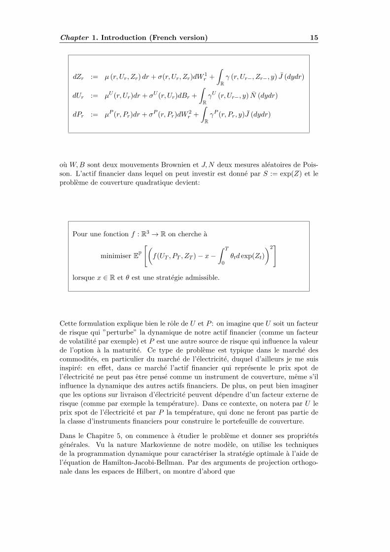
dZr := µ (r, Ur, Zr) dr + σ(r, Ur, Zr)dW1r +
∫Rγ (r, Ur−, Zr−, y) J (dydr)
dUr := µU (r, Ur)dr + σU (r, Ur)dBr +
∫RγU (r, Ur−, y) N (dydr)
dPr := µP (r, Pr)dr + σP (r, Pr)dW2r +
∫RγP (r, Pr, y)J (dydr)
ou W,B sont deux mouvements Brownien et J,N deux mesures aleatoires de Pois-son. L’actif financier dans lequel on peut investir est donne par S := exp(Z) et leprobleme de couverture quadratique devient:
Pour une fonction f : R3 → R on cherche a
minimiser EP
[(f(UT , PT , ZT )− x−
∫ T
0θtd exp(Zt)
)2]
lorsque x ∈ R et θ est une strategie admissible.
Cette formulation explique bien le role de U et P : on imagine que U soit un facteurde risque qui ”perturbe” la dynamique de notre actif financier (comme un facteurde volatilite par exemple) et P est une autre source de risque qui influence la valeurde l’option a la maturite. Ce type de probleme est typique dans le marche descommodites, en particulier du marche de l’electricite, duquel d’ailleurs je me suisinspire: en effet, dans ce marche l’actif financier qui represente le prix spot del’electricite ne peut pas etre pense comme un instrument de couverture, meme s’ilinfluence la dynamique des autres actifs financiers. De plus, on peut bien imaginerque les options sur livraison d’electricite peuvent dependre d’un facteur externe derisque (comme par exemple la temperature). Dans ce contexte, on notera par U leprix spot de l’electricite et par P la temperature, qui donc ne feront pas partie dela classe d’instruments financiers pour construire le portefeuille de couverture.
Dans le Chapitre 5, on commence a etudier le probleme et donner ses proprietesgenerales. Vu la nature Markovienne de notre modele, on utilise les techniquesde la programmation dynamique pour caracteriser la strategie optimale a l’aide del’equation de Hamilton-Jacobi-Bellman. Par des arguments de projection orthogo-nale dans les espaces de Hilbert, on montre d’abord que
16 Chapter 1. Introduction (French version)
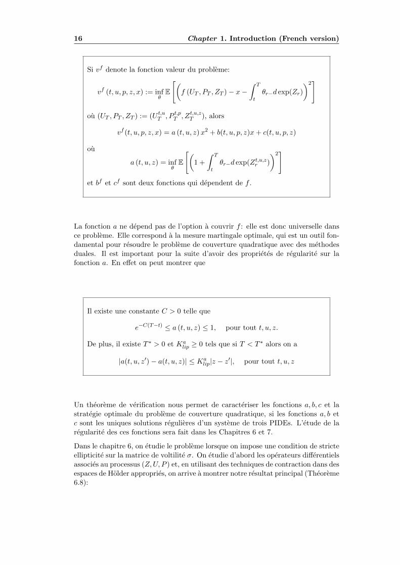
Si vf denote la fonction valeur du probleme:
vf (t, u, p, z, x) := infθE
[(f (UT , PT , ZT )− x−
∫ T
tθr−d exp(Zr)
)2]
ou (UT , PT , ZT ) := (U t,uT , P t,pT , Zt,u,zT ), alors
vf (t, u, p, z, x) = a (t, u, z)x2 + b(t, u, p, z)x+ c(t, u, p, z)
ou
a (t, u, z) = infθE
[(1 +
∫ T
tθr−d exp(Zt,u,zr )
)2]
et bf et cf sont deux fonctions qui dependent de f .
La fonction a ne depend pas de l’option a couvrir f : elle est donc universelle dansce probleme. Elle correspond a la mesure martingale optimale, qui est un outil fon-damental pour resoudre le probleme de couverture quadratique avec des methodesduales. Il est important pour la suite d’avoir des proprietes de regularite sur lafonction a. En effet on peut montrer que
Il existe une constante C > 0 telle que
e−C(T−t) ≤ a (t, u, z) ≤ 1, pour tout t, u, z.
De plus, il existe T ∗ > 0 et Kalip ≥ 0 tels que si T < T ∗ alors on a
|a(t, u, z′)− a(t, u, z)| ≤ Kalip|z − z′|, pour tout t, u, z
Un theoreme de verification nous permet de caracteriser les fonctions a, b, c et lastrategie optimale du probleme de couverture quadratique, si les fonctions a, b etc sont les uniques solutions regulieres d’un systeme de trois PIDEs. L’etude de laregularite des ces fonctions sera fait dans les Chapitres 6 et 7.
Dans le chapitre 6, on etudie le probleme lorsque on impose une condition de stricteellipticite sur la matrice de voltilite σ. On etudie d’abord les operateurs differentielsassocies au processus (Z,U, P ) et, en utilisant des techniques de contraction dans desespaces de Holder appropries, on arrive a montrer notre resultat principal (Theoreme6.8):
Chapter 1. Introduction (French version) 17
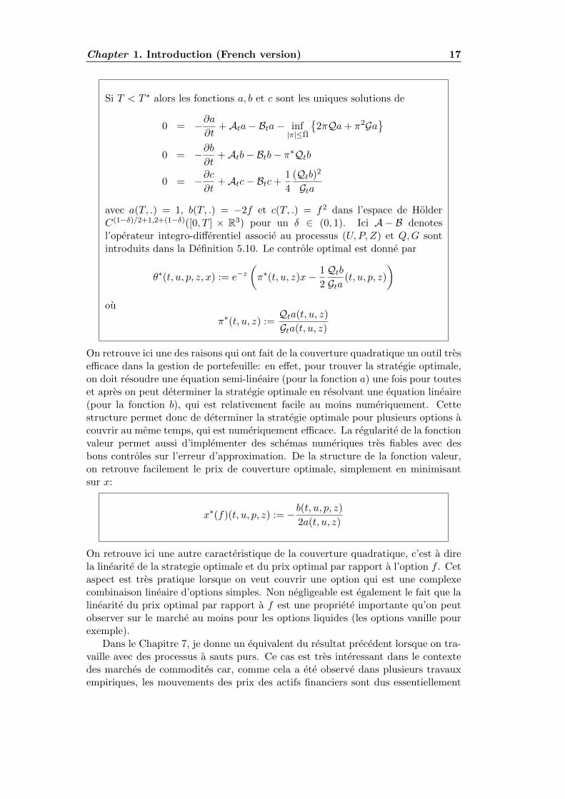
Si T < T ∗ alors les fonctions a, b et c sont les uniques solutions de
0 = −∂a∂t
+Ata− Bta− inf|π|≤Π
2πQa+ π2Ga
0 = −∂b
∂t+Atb− Btb− π∗Qtb
0 = −∂c∂t
+Atc− Btc+1
4
(Qtb)2
Gta
avec a(T, .) = 1, b(T, .) = −2f et c(T, .) = f2 dans l’espace de HolderC(1−δ)/2+1,2+(1−δ)([0, T ] × R3) pour un δ ∈ (0, 1). Ici A− B denotesl’operateur integro-differentiel associe au processus (U,P, Z) et Q,G sontintroduits dans la Definition 5.10. Le controle optimal est donne par
θ∗(t, u, p, z, x) := e−z(π∗(t, u, z)x− 1
2
QtbGta
(t, u, p, z)
)ou
π∗(t, u, z) :=Qta(t, u, z)
Gta(t, u, z)
On retrouve ici une des raisons qui ont fait de la couverture quadratique un outil tresefficace dans la gestion de portefeuille: en effet, pour trouver la strategie optimale,on doit resoudre une equation semi-lineaire (pour la fonction a) une fois pour touteset apres on peut determiner la strategie optimale en resolvant une equation lineaire(pour la fonction b), qui est relativement facile au moins numeriquement. Cettestructure permet donc de determiner la strategie optimale pour plusieurs options acouvrir au meme temps, qui est numeriquement efficace. La regularite de la fonctionvaleur permet aussi d’implementer des schemas numeriques tres fiables avec desbons controles sur l’erreur d’approximation. De la structure de la fonction valeur,on retrouve facilement le prix de couverture optimale, simplement en minimisantsur x:
x∗(f)(t, u, p, z) := −b(t, u, p, z)2a(t, u, z)
On retrouve ici une autre caracteristique de la couverture quadratique, c’est a direla linearite de la strategie optimale et du prix optimal par rapport a l’option f . Cetaspect est tres pratique lorsque on veut couvrir une option qui est une complexecombinaison lineaire d’options simples. Non negligeable est egalement le fait que lalinearite du prix optimal par rapport a f est une propriete importante qu’on peutobserver sur le marche au moins pour les options liquides (les options vanille pourexemple).
Dans le Chapitre 7, je donne un equivalent du resultat precedent lorsque on tra-vaille avec des processus a sauts purs. Ce cas est tres interessant dans le contextedes marches de commodites car, comme cela a ete observe dans plusieurs travauxempiriques, les mouvements des prix des actifs financiers sont dus essentiellement
18 Chapter 1. Introduction (French version)
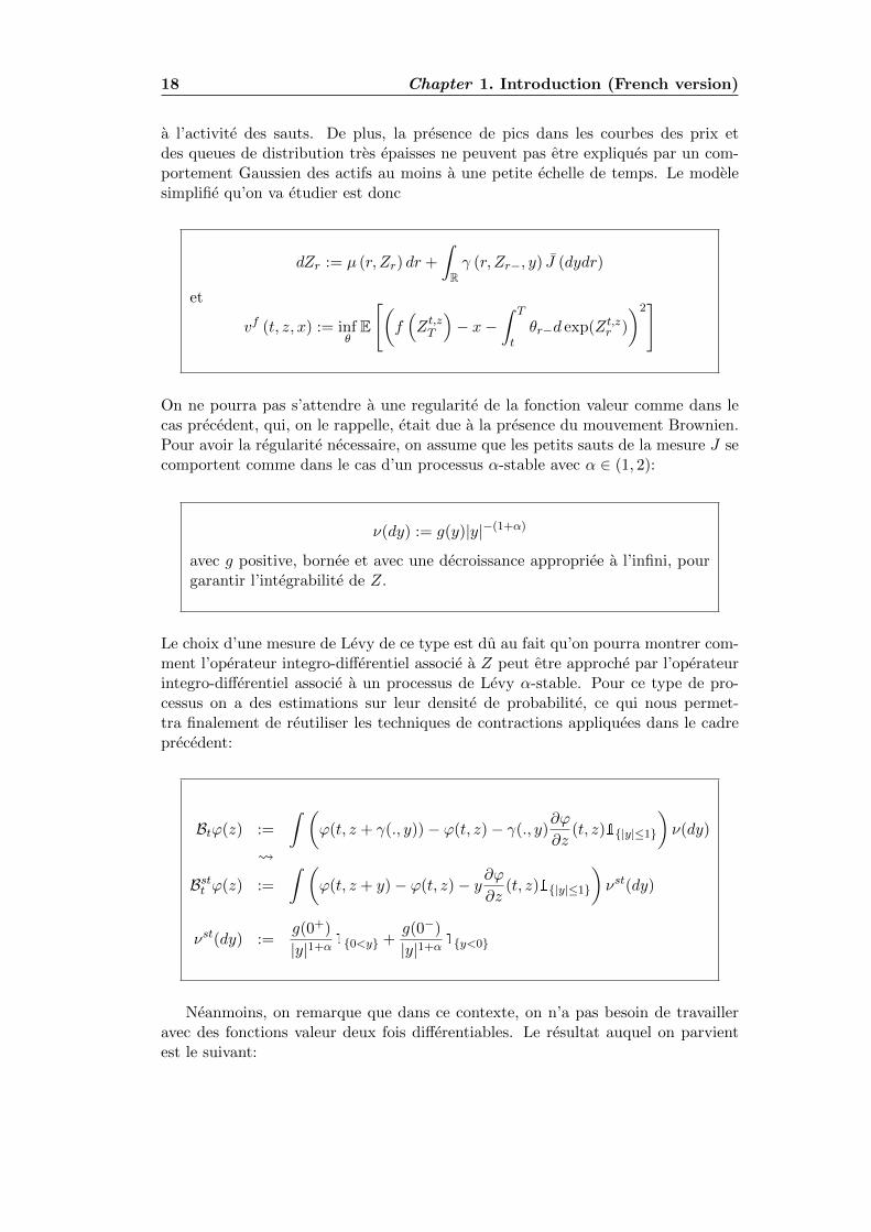
a l’activite des sauts. De plus, la presence de pics dans les courbes des prix etdes queues de distribution tres epaisses ne peuvent pas etre expliques par un com-portement Gaussien des actifs au moins a une petite echelle de temps. Le modelesimplifie qu’on va etudier est donc
dZr := µ (r, Zr) dr +
∫Rγ (r, Zr−, y) J (dydr)
et
vf (t, z, x) := infθE
[(f(Zt,zT
)− x−
∫ T
tθr−d exp(Zt,zr )
)2]
On ne pourra pas s’attendre a une regularite de la fonction valeur comme dans lecas precedent, qui, on le rappelle, etait due a la presence du mouvement Brownien.Pour avoir la regularite necessaire, on assume que les petits sauts de la mesure J secomportent comme dans le cas d’un processus α-stable avec α ∈ (1, 2):
ν(dy) := g(y)|y|−(1+α)
avec g positive, bornee et avec une decroissance appropriee a l’infini, pourgarantir l’integrabilite de Z.
Le choix d’une mesure de Levy de ce type est du au fait qu’on pourra montrer com-ment l’operateur integro-differentiel associe a Z peut etre approche par l’operateurintegro-differentiel associe a un processus de Levy α-stable. Pour ce type de pro-cessus on a des estimations sur leur densite de probabilite, ce qui nous permet-tra finalement de reutiliser les techniques de contractions appliquees dans le cadreprecedent:
Btϕ(z) :=
∫ (ϕ(t, z + γ(., y))− ϕ(t, z)− γ(., y)
∂ϕ
∂z(t, z)1|y|≤1
)ν(dy)
Bstt ϕ(z) :=
∫ (ϕ(t, z + y)− ϕ(t, z)− y∂ϕ
∂z(t, z)1|y|≤1
)νst(dy)
νst(dy) :=g(0+)
|y|1+α10<y +
g(0−)
|y|1+α1y<0
Neanmoins, on remarque que dans ce contexte, on n’a pas besoin de travailleravec des fonctions valeur deux fois differentiables. Le resultat auquel on parvientest le suivant:
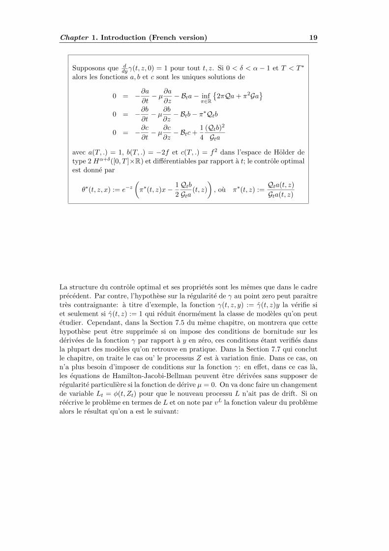
Chapter 1. Introduction (French version) 19
Supposons que ddyγ(t, z, 0) = 1 pour tout t, z. Si 0 < δ < α − 1 et T < T ∗
alors les fonctions a, b et c sont les uniques solutions de
0 = −∂a∂t− µ∂a
∂z− Bta− inf
π∈R
2πQa+ π2Ga
0 = −∂b
∂t− µ∂b
∂z− Btb− π∗Qtb
0 = −∂c∂t− µ∂c
∂z− Btc+
1
4
(Qtb)2
Gta
avec a(T, .) = 1, b(T, .) = −2f et c(T, .) = f2 dans l’espace de Holder detype 2 Hα+δ([0, T ]×R) et differentiables par rapport a t; le controle optimalest donne par
θ∗(t, z, x) := e−z(π∗(t, z)x− 1
2
QtbGta
(t, z)
), ou π∗(t, z) :=
Qta(t, z)
Gta(t, z)
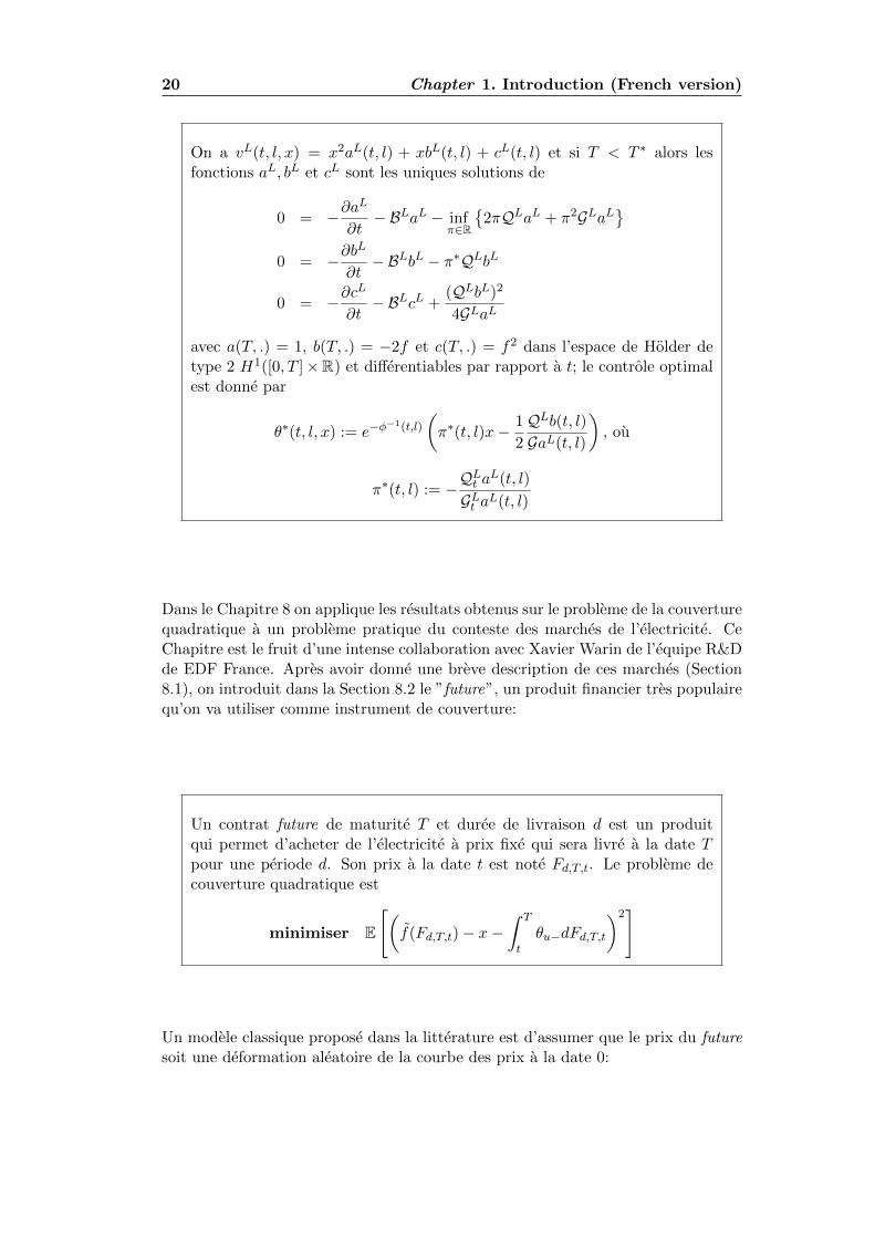
La structure du controle optimal et ses proprietes sont les memes que dans le cadreprecedent. Par contre, l’hypothese sur la regularite de γ au point zero peut paraıtretres contraignante: a titre d’exemple, la fonction γ(t, z, y) := γ(t, z)y la verifie siet seulement si γ(t, z) := 1 qui reduit enormement la classe de modeles qu’on peutetudier. Cependant, dans la Section 7.5 du meme chapitre, on montrera que cettehypothese peut etre supprimee si on impose des conditions de bornitude sur lesderivees de la fonction γ par rapport a y en zero, ces conditions etant verifies dansla plupart des modeles qu’on retrouve en pratique. Dans la Section 7.7 qui conclutle chapitre, on traite le cas ou’ le processus Z est a variation finie. Dans ce cas, onn’a plus besoin d’imposer de conditions sur la fonction γ: en effet, dans ce cas la,les equations de Hamilton-Jacobi-Bellman peuvent etre derivees sans supposer deregularite particuliere si la fonction de derive µ = 0. On va donc faire un changementde variable Lt = φ(t, Zt) pour que le nouveau processu L n’ait pas de drift. Si onreecrive le probleme en termes de L et on note par vL la fonction valeur du problemealors le resultat qu’on a est le suivant:
20 Chapter 1. Introduction (French version)
On a vL(t, l, x) = x2aL(t, l) + xbL(t, l) + cL(t, l) et si T < T ∗ alors lesfonctions aL, bL et cL sont les uniques solutions de
0 = −∂aL
∂t− BLaL − inf
π∈R
2πQLaL + π2GLaL
0 = −∂b
L
∂t− BLbL − π∗QLbL
0 = −∂cL
∂t− BLcL +
(QLbL)2
4GLaL
avec a(T, .) = 1, b(T, .) = −2f et c(T, .) = f2 dans l’espace de Holder detype 2 H1([0, T ]×R) et differentiables par rapport a t; le controle optimalest donne par
θ∗(t, l, x) := e−φ−1(t,l)
(π∗(t, l)x− 1
2
QLb(t, l)GaL(t, l)
), ou
π∗(t, l) := −QLt a
L(t, l)
GLt aL(t, l)
Dans le Chapitre 8 on applique les resultats obtenus sur le probleme de la couverturequadratique a un probleme pratique du conteste des marches de l’electricite. CeChapitre est le fruit d’une intense collaboration avec Xavier Warin de l’equipe R&Dde EDF France. Apres avoir donne une breve description de ces marches (Section8.1), on introduit dans la Section 8.2 le ”future”, un produit financier tres populairequ’on va utiliser comme instrument de couverture:
Un contrat future de maturite T et duree de livraison d est un produitqui permet d’acheter de l’electricite a prix fixe qui sera livre a la date Tpour une periode d. Son prix a la date t est note Fd,T,t. Le probleme decouverture quadratique est
minimiser E
[(f(Fd,T,t)− x−
∫ T
tθu−dFd,T,t
)2]
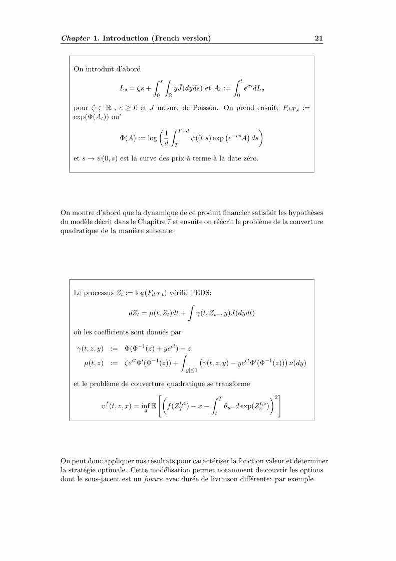
Un modele classique propose dans la litterature est d’assumer que le prix du futuresoit une deformation aleatoire de la courbe des prix a la date 0:
Chapter 1. Introduction (French version) 21
On introduit d’abord
Ls = ζs+
∫ s
0
∫RyJ(dyds) et At :=
∫ t
0ecsdLs
pour ζ ∈ R , c ≥ 0 et J mesure de Poisson. On prend ensuite Fd,T,t :=exp(Φ(At)) ou’
Φ(A) := log
(1
d
∫ T+d
Tψ(0, s) exp
(e−csA
)ds
)et s→ ψ(0, s) est la curve des prix a terme a la date zero.
On montre d’abord que la dynamique de ce produit financier satisfait les hypothesesdu modele decrit dans le Chapitre 7 et ensuite on reecrit le probleme de la couverturequadratique de la maniere suivante:
Le processus Zt := log(Fd,T,t) verifie l’EDS:
dZt = µ(t, Zt)dt+
∫γ(t, Zt−, y)J(dydt)
ou les coefficients sont donnes par
γ(t, z, y) := Φ(Φ−1(z) + yect)− z
µ(t, z) := ζectΦ′(Φ−1(z)) +
∫|y|≤1
(γ(t, z, y)− yectΦ′(Φ−1(z))
)ν(dy)
et le probleme de couverture quadratique se transforme
vf (t, z, x) = infθE
[(f(Zt,zT )− x−
∫ T
tθu−d exp(Zt,zs )
)2]
On peut donc appliquer nos resultats pour caracteriser la fonction valeur et determinerla strategie optimale. Cette modelisation permet notamment de couvrir les optionsdont le sous-jacent est un future avec duree de livraison differente: par exemple
22 Chapter 1. Introduction (French version)
Soit p(x) = (G− x)+, d′ 6= d et
h(A) :=1
d′
∫ T+d′
Tψ(0, s)eg(s)Ads
Il s’ensuit que h Φ−1(Zt) = Fd′,T,t. En particulier, le probleme de couver-ture quadratique pour f = p h Φ−1(Zt) devient
minimiserE
[((G− Fd′,T,t)+ − x−
∫ T
tθu−dFd,T,u
)2]
ce qui correspond a couvrir une option put dont le sous-jacent est Fd′,Tavec un portefeuille compose de contrats futures avec duree de livraisond. Cet aspect est interessant lorsque on veut couvrir des options dont lesous-jacent n’est pas echange sur le marche (en effet, les future qui sontechanges sur le marche ont des durees de livraison standardisees, 1 mois, 3mois, etc.).
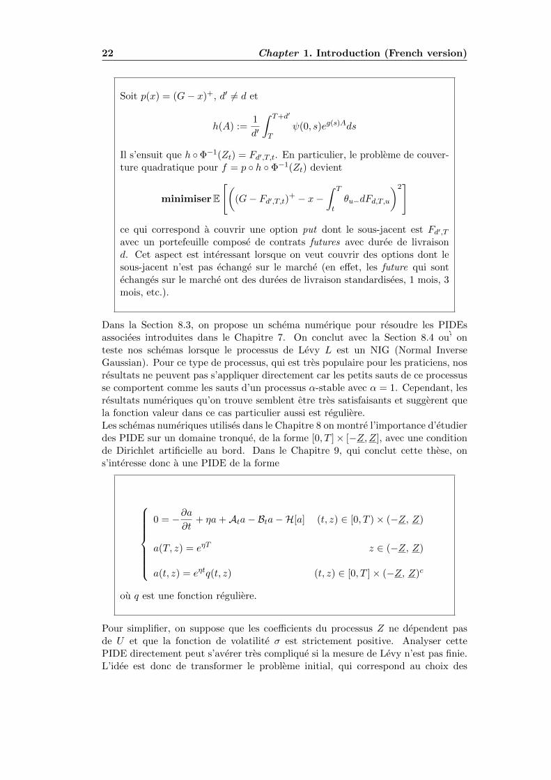
Dans la Section 8.3, on propose un schema numerique pour resoudre les PIDEsassociees introduites dans le Chapitre 7. On conclut avec la Section 8.4 ou’ onteste nos schemas lorsque le processus de Levy L est un NIG (Normal InverseGaussian). Pour ce type de processus, qui est tres populaire pour les praticiens, nosresultats ne peuvent pas s’appliquer directement car les petits sauts de ce processusse comportent comme les sauts d’un processus α-stable avec α = 1. Cependant, lesresultats numeriques qu’on trouve semblent etre tres satisfaisants et suggerent quela fonction valeur dans ce cas particulier aussi est reguliere.Les schemas numeriques utilises dans le Chapitre 8 on montre l’importance d’etudierdes PIDE sur un domaine tronque, de la forme [0, T ]× [−Z,Z], avec une conditionde Dirichlet artificielle au bord. Dans le Chapitre 9, qui conclut cette these, ons’interesse donc a une PIDE de la forme
0 = −∂a∂t
+ ηa+Ata− Bta−H[a] (t, z) ∈ [0, T )× (−Z, Z)
a(T, z) = eηT z ∈ (−Z, Z)
a(t, z) = eηtq(t, z) (t, z) ∈ [0, T ]× (−Z, Z)c
ou q est une fonction reguliere.
Pour simplifier, on suppose que les coefficients du processus Z ne dependent pasde U et que la fonction de volatilite σ est strictement positive. Analyser cettePIDE directement peut s’averer tres complique si la mesure de Levy n’est pas finie.L’idee est donc de transformer le probleme initial, qui correspond au choix des
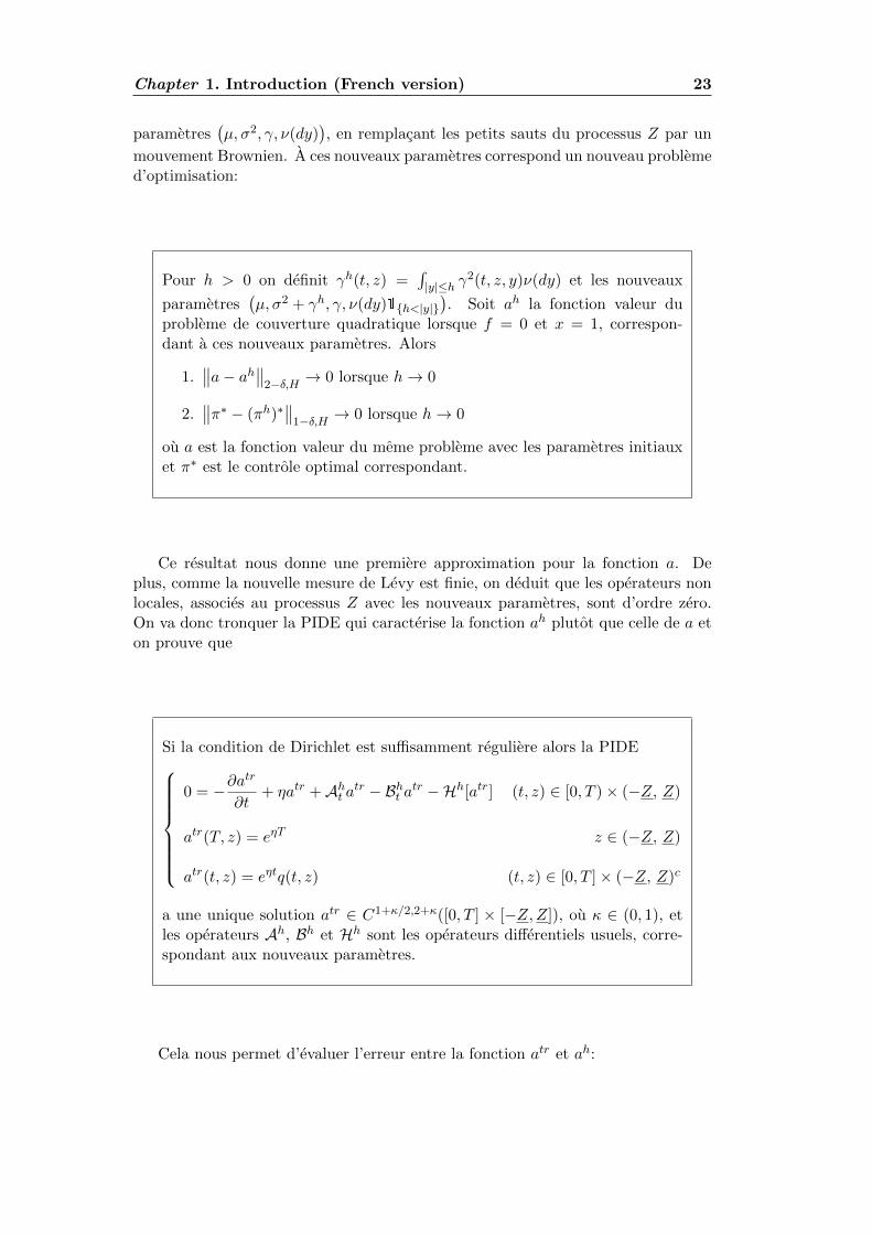
Chapter 1. Introduction (French version) 23
parametres(µ, σ2, γ, ν(dy)
), en remplacant les petits sauts du processus Z par un
mouvement Brownien. A ces nouveaux parametres correspond un nouveau problemed’optimisation:
Pour h > 0 on definit γh(t, z) =∫|y|≤h γ
2(t, z, y)ν(dy) et les nouveaux
parametres(µ, σ2 + γh, γ, ν(dy)1h<|y|
). Soit ah la fonction valeur du
probleme de couverture quadratique lorsque f = 0 et x = 1, correspon-dant a ces nouveaux parametres. Alors
1.∥∥a− ah∥∥
2−δ,H → 0 lorsque h→ 0
2.∥∥π∗ − (πh)∗
∥∥1−δ,H → 0 lorsque h→ 0
ou a est la fonction valeur du meme probleme avec les parametres initiauxet π∗ est le controle optimal correspondant.
Ce resultat nous donne une premiere approximation pour la fonction a. Deplus, comme la nouvelle mesure de Levy est finie, on deduit que les operateurs nonlocales, associes au processus Z avec les nouveaux parametres, sont d’ordre zero.On va donc tronquer la PIDE qui caracterise la fonction ah plutot que celle de a eton prouve que
Si la condition de Dirichlet est suffisamment reguliere alors la PIDE
0 = −∂atr
∂t+ ηatr +Aht atr − Bht atr −Hh[atr] (t, z) ∈ [0, T )× (−Z, Z)
atr(T, z) = eηT z ∈ (−Z, Z)
atr(t, z) = eηtq(t, z) (t, z) ∈ [0, T ]× (−Z, Z)c
a une unique solution atr ∈ C1+κ/2,2+κ([0, T ] × [−Z,Z]), ou κ ∈ (0, 1), etles operateurs Ah, Bh et Hh sont les operateurs differentiels usuels, corre-spondant aux nouveaux parametres.
Cela nous permet d’evaluer l’erreur entre la fonction atr et ah:
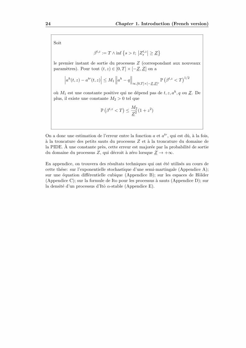
24 Chapter 1. Introduction (French version)
Soit
βt,z := T ∧ infs > t;
∣∣Zt,zs ∣∣ ≥ Zle premier instant de sortie du processus Z (correspondant aux nouveauxparametres). Pour tout (t, z) ∈ [0, T ]× [−Z,Z] on a∣∣∣ah(t, z)− atr(t, z)
∣∣∣ ≤M1
∥∥∥ah − q∥∥∥∞,[0,T ]×[−Z,Z]c
P(βt,z < T
)1/2ou M1 est une constante positive qui ne depend pas de t, z, ah, q ou Z. Deplus, il existe une constante M2 > 0 tel que
P(βt,z < T
)≤ M2
Z2 (1 + z2)
On a donc une estimation de l’erreur entre la fonction a et atr, qui est du, a la fois,a la troncature des petits sauts du processus Z et a la troncature du domaine dela PIDE. A une constante pres, cette erreur est majoree par la probabilite de sortiedu domaine du processus Z, qui decroit a zero lorsque Z → +∞.
En appendice, on trouvera des resultats techniques qui ont ete utilises au cours decette these: sur l’exponentielle stochastique d’une semi-martingale (Appendice A);sur une equation differentielle cubique (Appendice B); sur les espaces de Holder(Appendice C); sur la formule de Ito pour les processus a sauts (Appendice D); surla densite d’un processus d’Ito α-stable (Appendice E).
Chapter 2
Introduction
The main object of this thesis is to propose, investigate and solve some problemson portfolio management theory. The work is composed of two parts. In the firstone we propose a new problem concerning the utility maximization theory, wherethe usual convex structure of the problem is removed (by a modification of themaximization criterion) and a new type of constraint is imposed on the admissiblestrategies, inspired by portfolio insurance problems. In the second one we solvethe quadratic hedge problem for a class of discontinuous Markovian models whichturns out to be well adapted in the context of commodities markets, which partiallyinspired this work. The mathematical tools and the methodologies used in the twoparts are completely different. In the first one we privilege the so called ”dual”formulation which is more adapted in the context of utility maximization theorywhen the market is complete, whereas in the second one, where no assumptions aremade on the completeness on the market, we exploit the Markovian structure of themodel in order to implement the well known dynamic programming principle andthe relative Hamilton-Jacobi-Bellman equations.
The thesis starts with a brief but sufficiently complete introduction on risk mea-sures (Chapter 3), which have become an important tool in finance. After a shortdiscussion of their properties (Sections 3.1–3.2) we recall some of the most popularrisk measures: the Value at Risk VaR, the Conditional Value at Risk CVaR andmore generally the spectral risk measures (Section 3.3); the entropic risk measureand the G-divergence (Section 3.4). These special risk measures present many niceproperties and are analytically tractable, so that they will be used to deduce explicitresults in our non-standard utility maximization problem. The problem is presentedin Chapter 4 and in Section 4.2 we develop our methodology to solve it and pro-pose its solution. An important issue of this chapter is to show how the problemmay fail to have a finite solution if the risk measure does not fill a non-degeneracyassumption. For this we provide a criterion, easy to check, which guarantees theexistence of a finite solution and an algorithm to explicitly compute the optimal so-lution. We then start to test our results on practical examples: in Section 4.4 we usethe entropic risk measure and we provide a simple numerical experiment; Section4.5 is devoted to the study of the maximization problem when one uses a generalspectral risk measure and we provide a criterion under which the problem has afinite solution. The special case of the CVaR is treated in Paragraph 4.5.3, whereasthe G-divergence case is studied in Section 4.6. Section 4.7, which concludes the
25
26 Chapter 2. Introduction
chapter, is devoted to a comparison with other types of portfolio insurance whichhave been studied in the literature.
The second part of the thesis is devoted to the quadratic hedge problem fordiscontinuous Markovian models. The problem in all its generality is presented inChapter 5, starting by a short survey on what is already done in the literature (Sec-tion 5.1) and what is new in our work. As already pointed out in many previousworks, a fundamental step to solve the quadratic hedge problem is the so called pureinvestment problem: basically it is the quadratic hedge problem when one wantsto hedge the option with payoff f = 0. Both the quadratic hedge and the pureinvestment problem are introduced in Section 5.2 together with a general class ofMarkovian models used in the thesis. The model consists of a three-dimensionalprocess (Z,U, P ), where exp(Z) is the hedging instrument traded in the market, Uis a risk factor in the dynamics of Z which cannot be used as a hedging instrument(as a volatility factor for example) whereas P is another factor of risk which influ-ences the option one wants to hedge and is also not traded in the market. In Section5.3 we recall many properties of the value function corresponding to the pure in-vestment problem, and we use them to prove that it is uniformly bounded frombelow by a strictly positive constant, and Lipschitz continuous, whereas Section 5.4shows many general properties on the structure of the quadratic hedge problem.In Sections 5.5, we first introduce the integro-differential operators related to theMarkovian discontinuous model, and then we characterize the value function of thepure investment problems as the solution of a semi linear PIDE, provided that thisPIDE has a unique smooth solution. This is done with a verification argument, andit also give us the optimal strategy for the pure investment problem. We repeat thisprocedure in Section 5.6 for the value function of the quadratic hedge problem. Theexistence and uniqueness of the solution of these PIDEs are studied in Chapters6–7. We finally give a survey on the viscosity solution theory and see how it can beused in our context (Section 5.7).
In Chapter 6 we assume that the Markovian model used in the quadratic hedgeproblem is a non degenerate jump-diffusion, which is done by assuming strict el-lipticity on the matrix of the Brownian component. Section 6.1 is devoted to thestudy of the integro-differential operators associated to the jump-diffusion model:in particular we focus on their behavior when one considers them as operators in anappropriate Holder space. We obtain some fundamental results on their continuityin this space. In Section 6.2, we expose the methodology we use to prove that theHJB equation corresponding to the value function of the pure investment problemhas a unique solution in a Holder space of smooth functions. The proof is a mixtureof contraction techniques in Banach spaces (classical tool for specialists in differen-tial equations) and probabilistic techniques. Other methods to solve this problemare discussed in Paragraph 6.2.4, especially the ones making use of Backward SDEsor Sobolev spaces. Once one knows the value function of the pure investment prob-lem, it is straightforward to characterize the value function of the quadratic hedgeproblem. In Section 6.3 we prove our main result concerning the quadratic hedgeproblem for jump-diffusion models: its value function can be characterized as thesolution of a triplet of Partial integro-differential equations, the first of which is semilinear and it corresponds to the value function of the pure investment problem; theother two are linear, so relatively easy to solve (at least numerically).
Chapter 2. Introduction 27
The results of Chapter 6 are derived by assuming, in particular, that the matrixof the Brownian component is strictly elliptic. This assumption seems to be veryrestrictive if one wants to apply our results, for example, to the quadratic hedgeproblem in commodities markets. In these markets, it is popular to model thestock price as a purely discontinuous process, which basically corresponds to assumethat Brownian component is equal to zero. Motivated by many discussions withpractitioners in commodities markets, in Chapter 7 we assume that the stock priceprocess is driven by a Poisson random measure. We start Chapter 7 by introducinga pure jump model for the stock price used for the quadratic hedge problem, forwhich we assume some properties on its Levy measure (Section 7.1). In particularwe assume that the small jumps of the process ”look like” the jumps of an α-stableprocess, i.e. the Levy measure has a density w.r.t. the Lebesgue measure, which isassumed to be a weighted deformation of the density of an α-stable Levy processwith α ∈ (1, 2). This is done since many properties are known for these processes,in particular on their density, and this will allow us to prove the smoothness of thevalue function. We proceed then as in Chapter 6 by studying the integro-differentialoperators in a new functional space that we call Holder space of type 2. This isdone since in the pure jump case we cannot expect the same regularity for the valuefunction as before. The fundamental result in this case is that we can replace theprincipal term of the HJB solved by the value function with the integro-differentialoperator associated to an α-stable Levy process, for which we know many properties(Paragraph 7.3). We prove (Paragraphs 7.4.1–7.4.2) that the value function of thepure investment problem can be characterized as the unique smooth solution in anappropriate Holder space of type 2 of a semi linear PIDE. We can finally characterizethe value function of the quadratic hedge problem in the pure jump case (Section7.6), and, as in Chapter 6, we find that it solves a triplet of semi linear PIDEs.Section 7.7, which concludes the chapter, is devoted to the study of the problemwhen the stock price is modeled by a finite variation pure jump process (whichincludes the case α ∈ (0, 1) excluded before): in this relatively simple case we alsofind that the value function is characterized by a triplet of PIDEs which have aunique solution in the space of Lipschitz continuous functions.
We can finally apply the results provided in Chapter 7 on a practical problemfrom the portfolio management in electricity markets. Chapter 8 summarizes anintense and fruitful collaboration with Xavier Warin of R&D department of EDFFrance. We first discuss why financial instruments in electricity markets are gener-ally modeled by pure jump processes (Section 8.1) and then we present the futurecontract, a popular hedging instrument in these markets (Section 8.2). Section 8.3is devoted to the numerical methodology used to solve the PIDEs related to thevalue function of the quadratic hedge problem. We conclude the Chapter by usingthese schemes when the future contract is modeled as a random deformation of theforward curve, the randomness coming from a NIG process, which corresponds tothe case α = 1 in Chapter 7. Although for this case we cannot directly apply ourresult and then it should be considered as a degenerate case in some sense, thenumerical results that we obtain are encouraging. In particular we obtain a numer-ical approximation for the value function of the pure investment problem and itsoptimal control and the profiles for the value functions of an at-the-money call andput options written on the future contract.
28 Chapter 2. Introduction
The numerical schemes used in Chapter 8 showed that it is important to studythe PIDEs on a bounded domain and to quantify the truncation error. We do thisanalysis in Chapter 9 where, to simplify, we assume that the process Z does notdepend on U . In a general framework it is not easy to study these PIDEs on abounded domain, unless one assumes that the intensity measure of the process Z isfinite. Since the method can be readapted for all the PIDEs, we just study the PIDEcharacterizing the value function of the pure investment problem a. We provide afirst approximation of this value function by cutting the small jumps of the processZ and replacing them with a Brownian motion. This is equivalent to consider themodel with new parameters, where, in particular, one has a finite intensity measure.This new model leads to a new value function of the pure investment problem and inSection 9.2 we are able to give an estimate on the error between the value functiona and the new value function, and prove that we can make this error as smallas we want, provided that the level at which we cut the jumps is small enough.Once we have approximated this value function, we concentrate on the PIDE thatcharacterizes this new value function. We first prove that the truncated versionof this PIDE also has a unique smooth solution (Section 9.3) and finally give anestimate on the error between the new value function and the unique solution ofthe truncated PIDE (Section 9.4).
We conclude the thesis with several appendices in which one can find manyinteresting technical results that we used throughout the thesis: on stochastic ex-ponentials for semimartingales (Appendix A); on a cubic differential equation (Ap-pendix B); on Holder spaces (Appendix C); on Ito’s formula for pure jump processes(Appendix D) and on the density of α-stable Levy processes (Appendix E).

Part I
Portfolio Insurance under riskmeasure constraint
29

Chapter 3
An overview on Risk measures
In this chapter we will recall the axiomatic definition of risk measures and theirmain properties (Section 3.2). We then describe some of the most popular riskmeasures used in finance: the Value-at-Risk (VaR), the Conditional Value-at-Risk(CVaR) and, more generally, the spectral risk measures (Section 3.3); the Entropicrisk measure and the G-divergence (Section 3.4). Since we are more interested inthe use of them in risk management, we restrict ourselves to a brief survey on theiraxiomatic definition and their main properties. Excellent works on the subject canbe found in our references.
Contents
3.1 Practical needs of the risk measures: empirical evidence 313.2 Law invariant risk measures . . . . . . . . . . . . . . . . . 32
3.2.1 Definition and main properties . . . . . . . . . . . . . . . 323.2.2 Representation of convex risk measures . . . . . . . . . . 33
3.3 VaR, CVaR and spectral risk measures . . . . . . . . . . 353.4 G-divergence and entropy . . . . . . . . . . . . . . . . . . 373.5 Risk Measures on Lp-spaces . . . . . . . . . . . . . . . . . 38
3.1 Practical needs of the risk measures: empirical ev-idence
The last decade of 1980 has seen the increasing interest for risk measures. Ex-plicit references to them can be found in many reports by the Basel Committee ofBanking Supervision (BCBS) and the well known Basel accords (Basel Committee,1996, 2004). The main objective was to find a way to measure the exposure to risksfor investors, banks, and, more generally, for financial institutions. They become afundamental tool in risk management for banks and insurance companies since theyuse them to compute, for example, minimal capital requirements:
[. . .]A significant innovation of the revised Framework is the greater useof assessments of risk provided by banks internal systems as inputs to capitalcalculations. In taking this step, the Committee is also putting forward a
31
32 Chapter 3. An overview on Risk measures
detailed set of minimum requirements designed to ensure the integrity of theseinternal risk assessments. [. . .]Basel Committee (2004)
The above citation suggests a way to define these risk measures: roughly speakinga risk measure can be thought as the extra capital one needs to add to her portfolioin order to have a new portfolio with zero risk. The question now is the following:what is a portfolio with zero risk? This procedure is not yet satisfactory but givesus an important property for any reasonable definition of risk measure: in orderto define it, one only needs to be able to identify the portfolios with zero risk. Inparticular two portfolios with the same risk should keep the same risk exposureif one adds the same amount of capital to both of them. Remark however thatdeciding which portfolios have zero risk is a subjective choice. Following these ideasArtzner et al. (1999) first gave a precise definition of what should be a reasonabledefinition of a risk measure.We want to give here a simple example of what should not be a good way to measurethe risk: assume that there are two portfolios, say P1 and P2, at time t = 0, suchthat at time t = 1 they have the following distribution:
P1 =
1 on the set A−1 on the set Ac
P2 =
100 on the set A−100 on the set Ac
where A is a set of possible scenarios with P(A) = 1/2. If we agree to measurethe portfolio’s risk with the probability of being negative then risk(P1) = risk(P2),whereas risk(P1 + 1) > risk(P2 + 1). It follows that adding the same amount toboth the portfolios changes their risk in a different way. This violate the propertyseen before that any reasonable risk measure should have. Remark that any investorwould agree that the portfolio P2 is more risky than P1, so that this way of measurethe portfolio’s risk is not reasonable.
3.2 Law invariant risk measures
3.2.1 Definition and main properties
We now present the construction of risk measures for bounded random variablesin the static case, by following the ideas of Follmer and Schied (2004). For thedynamic definition of risk measures we refer to Frittelli and Gianin (2004); Bion-Nadal (2008, 2009) and references therein. The use of quadratic BSDEs in thedynamic risk measures theory can be found in Barrieu and El Karoui (2004, 2008)and their related bibliography.Let (Ω, F , P) be a probability space and L∞ := L∞(Ω,P) the Banach space of (es-sentially) bounded random variable X : Ω→ R. The multidimensional case has tobe carefully treated because there are some non trivial technical difficulties; howeverthe main results that we will present can be extended in the multidimensional case(Jouini et al., 2004; Ekeland et al., 2009; Ekeland and Schachermayer, 2011).
Definition 3.1. A law invariant risk measure ρ on L∞(Ω) is a functional ρ :L∞(Ω)→ R verifying the following properties:
i). For any X ≤ Y P-a.s. ρ(X) ≥ ρ(Y ) (Monotonicity)
Chapter 3. An overview on Risk measures 33
ii). For any m ∈ R ρ(X +m) = ρ(X)−m (Cash Invariance)
We say that ρ is normalized if ρ(0) = 0. ρ is said to be law invariant if
ρ(X) = ρ(Y ) whenever XL= Y
From now on, except when mentioned, we consider all risk measures to be lawinvariant.
Definition 3.2. Let ρ be a risk measure on L∞(Ω).
i). We say that ρ is convex if for any λ ∈ [0, 1] and any X,Y ∈ L∞(Ω) one hasρ (λX + (1− λ)Y ) ≤ λρ (X) + (1− λ)ρ (Y ) .
ii). We say that a convex risk measure ρ is coherent if for any m ≥ 0 and anyX ∈ L∞(Ω) one has ρ(mX) = mρ(X)
The financial meaning of Definition 3.1 is clear. More interesting are the condi-tions given in Definition 3.2: condition i) essentially says that if the risk is measuredwith a convex risk measure ρ then diversification decreases the risk, whereas condi-tion ii) says that proportional portfolios have proportional risks.
The cash invariance and monotonicity property also gives that any risk measureis Lipschitz continuous : |ρ(X)− ρ(Y )| ≤ ‖X − Y ‖∞. An important object relatedto risk measures is the so called acceptance set :
Aρ := X ∈ L∞ | ρ(X) ≤ 0 (3.1)
This set has some interesting properties, in particular the fact that any risk measurecan be recovered from its acceptance set. We list here some properties of Aρ:
Lemma 3.3. Let X,Y ∈ L∞ and Aρ as in (3.1). Then:
i). If X ∈ Aρ and Y ≥ X then Y ∈ Aρ and inf x ∈ R | x ∈ Aρ > −∞
ii). ρ admits the representation :ρ(X) = inf x ∈ R | x+X ∈ Aρ
iii). If ρ is a convex risk measure then Aρ is a convex subset of L∞
iv). If ρ is a coherent risk measure then Aρ is a convex cone in L∞
Conversely, a risk measure can be defined from a suitable acceptance set: letA ⊆ L∞ be a set of bounded random variables which verifies the property i) ofLemma 3.3. Then the functional ρ defined in Lemma 3.3 iii) is a risk measure,which is convex if A is a cone, and coherent if A is a convex cone.
3.2.2 Representation of convex risk measures
In this paragraph we will recall some well known results on the representationof convex risk measures. We keep following Follmer and Schied (2004) and we referto them for the proofs. The general result is the following:
34 Chapter 3. An overview on Risk measures
Theorem 3.4. For any convex risk measure ρ (not necessarily law invariant) thereexists a functional γmin :M1,f → [0, 1], where M1,f is the set of normalized finiteadditive measures on F , such that
ρ(X) : supQ∈M1,f
(EQ [−X]− γmin (Q)
), X ∈ L∞
The functional γmin is called the minimal penalty function and it is related to ρ by
γmin (Q) := supX∈Aρ
EQ [−X] (3.2)
If ρ is coherent then γmin takes values in 0, +∞.
The above Theorem shows that any risk measure can be characterized by afunctional on M1,f . However it is preferable to have a representation for whichthe minimal penalty takes finite values only on true probabilities, which have to beσ−additive. This is possible if the risk measure has a regular behavior in the senseof the Definition below:
Definition 3.5. We say that a convex risk measure is continuous from below if forany Xn X we have ρ(Xn) ρ(X), Xn, X ∈ L∞. We say that it is continuousfrom above if for any Xn X we have ρ(Xn) ρ(X)
Theorem 3.6. Let ρ be a convex risk measure (not necessarily law invariant) con-tinuous from below. Then
ρ(X) : supQ∈M1
(EQ [−X]− γmin (Q)
), X ∈ L∞
where M1 is the set of probabilities on (Ω,F). In this case ρ is also continuousfrom above and satisfies the Fatou’s property
Xn → X P-a.s. then ρ(X) ≤ lim infn→∞
ρ(Xn)
Theorems 3.4–3.6 hold true for any convex risk measure not necessarily lawinvariant: when it is the case, the minimal penalty functional takes values in aparticular subset of M1:
Theorem 3.7. Let ρ be a law invariant convex risk measure. Then
ρ(X) : supQP
(EQ [−X]− γmin (Q)
), X ∈ L∞
if and only if ρ is continuous from above, or equivalently, if and only ρ has theFatou’s property
Xn → X P-a.s. then ρ(X) ≤ lim infn→∞
ρ(Xn)
In the next sections we will present some of the most popular risk measures andtheir main properties.
Chapter 3. An overview on Risk measures 35
3.3 VaR, CVaR and spectral risk measures
Let λ ∈ (0, 1) andX ∈ L∞. A λ-quantile ofX is a real number in[q−λ (X) , q+
λ (X)]
where
q−λ (X) := inf x ∈ R|P (X ≤ x) ≥ λq+λ (X) := sup x ∈ R|P (X < x) ≥ λ
Definition 3.8. The Value-at-Risk of X at level λ is defined as
V aRλ (X) :=− q+λ (X) = inf m ∈ R |P (X +m < 0) ≤ λ (3.3)
Equivalently we also have that V aRλ (X) = −F−1X (λ) where F−1
X is a generalized in-verse distribution function of X. Since the generalized inverse distribution functionhas at most a countable number of discontinuities, this definition does not dependon the particular choice of this function (right-continuous or left-continuous). Weshall always use the definition
F−1X (λ) := infx : F (x) ≥ λ (3.4)
with the convention inf ∅ = +∞.
It is not difficult to prove that the V aRλ is a law invariant risk measure. Manyexamples have shown that the V aR is not a convex risk measure. This feature hassome important financial consequences: in risk management diversification in theportfolio selection should decrease its risk, but if we measure this risk with the V aRthen this is not always the case.
Example 3.9. Let P1 and P2 the two portfolios in Section 3.1 and assume that P1
is independent from P2. It is easy to verify that
V aRλ(P1) =
1 if λ < 0.5−1 if λ ≥ 0.5
V aRλ(P2) =
100 if λ < 0.5−100 if λ ≥ 0.5
and
V aRλ(1
2P1 +
1
2P2) =
50.5 if 0 < λ < 0.2545.5 if 0.25 ≤ λ < 0.5−45.5 if 0.5 ≤ λ < 0.75−50.5 if 0.75 ≤ λ < 1
If now we take 0.5 ≤ λ < 0.75 we obtain
−45.5 = V aRλ(1
2P1 +
1
2P2) >
1
2V aRλ(P1) +
1
2V aRλ(P2) = −50.5
which shows that diversification does not decrease the risk.
In spite of the above example, the V aR is a popular risk measure which iswidely used by practitioners since it has a simple financial interpretation. Our firstexample of risk measure which is, at the same time, convex and simple to use, isthe so called Conditional Value-at-Risk:
36 Chapter 3. An overview on Risk measures
Definition 3.10. The Conditional Value-at-Risk of X at level λ is defined as
CV aRλ (X) :=1
λ
∫ λ
0V aRu (X) du = − 1
λ
∫ λ
0F−1X (u)du (3.5)
The following Proposition lists some properties of the CV aR:
Proposition 3.11. Let λ ∈ (0, 1). The CV aRλ is a coherent risk measure and itadmits the representation
CV aRλ (X) = supQ∈Hλ
EQ [−X] , Hλ :=
Q P | dQ
dP≤ 1
λP− a.s.
The supremum in the above representation is achieved by the probability
dQ∗
dP:=
1
λ
(1X<q + k1X=q
)where q is any λ-quantile in
[q−λ (X) , q+
λ (X)]
and
k =
0 if P (X = q) = 0
λ−P(X<q)P(X=q) otherwise
From the above Proposition we can determine the minimal penalty function for theCV aRλ:
γmin (Q) :=
0 if dQ
dP ≤1λ , P-a.s
+∞ otherwise(3.6)
It can also be proved that if (Ω, F , P) is atomless then the CV aR is the smallestlaw invariant convex risk measure to be continuous from below that dominates theV aR (Follmer and Schied, 2004).
Proposition 3.12. Let λ ∈ (0, 1), X ∈ L∞ and q be a λ-quantile for X in[q−λ (X) , q+
λ (X)]. Then
CV aRλ (X) =1
λinfs∈R
(E[(s−X)+
]− λs
)=
1
λE[(q −X)+
]− q
The representation given in Proposition 3.12 is much more simple to handle thenthe one given in Proposition 3.11, especially in risk management problems, since themaximization can be carried out over the real line instead of a set of probabilities.The CV aR is a special case of the so called spectral risk measure:
Definition 3.13. Let µ be a probability measure on (0, 1). The related spectral riskmeasure is defined as
ρµ (X) :=
∫ 1
0CV aRu (X)µ(du) (3.7)
It is straightforward to see that ρµ is a coherent risk measure continuous fromabove, since the CV aR is. In particular, if λ ∈ (0, 1) and µ(du) = δλ(du) thenρµ = CV aRλ. Furthermore, from the definition of CV aR we also can write
ρµ (X) :=
∫ 1
0µ(u)V aRu (X) du where µ(u) :=
∫ 1
u
µ(dx)
x(3.8)
The function µ is right-continuous, non increasing and normalized:∫ 1
0 µ(u)du = 1.
Chapter 3. An overview on Risk measures 37
Lemma 3.14. Let (ρi)i be a family of convex risk measures such that supi ρi(0) <+∞. Then
ρ(X) := supiρi(X)
is a convex risk measure.
Using Lemma 3.14 we can define a wide class of risk measures: for any subsetof probability measure M on (0, 1) the
ρM(X) := supµ∈M
∫ 1
0CV aRu(X)µ(du) (3.9)
is a coherent risk measure continuous from above. It can be proved that if (Ω, F , P)is atomless then any coherent risk measure continuous from above can be representedby a subset of probability measures on (0, 1) as in (3.9) (Follmer and Schied, 2004).
3.4 G-divergence and entropy
In this section we will introduce another class of risk measures which are par-ticularly simple to handle in risk management problems.Let G : R+ → R ∪ +∞ be a convex, increasing and non constant function,with G (1) < ∞ and G (x) /x → +∞ when x → +∞. The G−divergence of anyabsolutely continuous probability Q P is defined as
IG (Q | P) := E[G
(dQdP
)](3.10)
By using the G-divergence as penalty function in Theorem 3.6 we can build a newrisk measure (Csiszar, 1967):
ρG(X) := supQP
(EQ [−X]− IG (Q | P)
)(3.11)
The fact that G (x) /x → +∞ when x → +∞ and de la Vallee-Poussin’s criterion(See, for example, Doob (1994), Chapter VI, §17) show that the supremum in theabove definition is achieved by some probability measure Q∗. Furthermore, since Gis convex, a Lagrangian-type argument allows us to rewrite the above risk measureas
ρG(X) := infy∈R
(EP [G∗(y −X)]− y
)(3.12)
where G∗ (x) = supy>0 (yx−G (y)). For a detailed proof, see for example, Csiszar(1967); Liese and Vajda (1987); Follmer and Schied (2004). For example, if λ ∈ (0, 1)and
G (y) =
0 if 0 ≤ y ≤ 1
λ+∞ otherwise
then G∗ (y) =
yλ if y ≥ 00 otherwise
then
ρ (X) =1
λinfy∈R
(E[(y −X)+]− λy)
38 Chapter 3. An overview on Risk measures
which is nothing but the CV aRλ as stated in Proposition 3.12.
Another special case is given by G(x) := βx log(x) for β > 0: IG (Q | P) is thewell known entropy of Q with respect to P. The related entropic risk measure hasthe form
ρβ(X) := β logE[e−Xβ
](3.13)
Remark 3.15. A heuristic Taylor expansion yields
ρβ ≈ −E [X] +1
2βE[X2]
Small β implies high risk aversion.
3.5 Risk Measures on Lp-spaces
In risk management problems generally one has to deal with unbounded randomvariables. The domain of definition of ρ may be taken equal, for example, to someLp space (Kaina and Ruschendorf, 2009) or a more general Orlicz space (Section 5.4in Biagini and Frittelli (2009)). A general theory for risk measures on such spacesis available and a generalization of the representation given in Theorem 3.4 is alsoavailable. We do not go into details since it is not the scope of this thesis, however itis not difficult to extend the risk measures introduced in Sections 3.3–3.4 to L1(P).This extension is straightforward for the V aR, the CV aR and, more generally, forall spectral risk measures.
For the entropic risk measure we first remark that E [exp(−X/β)] is always welldefined and it may take the value +∞. Furthermore Jensen’s inequality yieldsρβ(X) ≥ −E [X]1, which allows us to extend the entropic risk measure to L1(P).Remark that now it takes values in (−∞,+∞]. A slight difference appears in thedual representation: if X ∈ L1(P) then we need to write
ρβ(X) := supQP,log( dQdP )∈L1(Q)
(EQ [−X]− EQ
[log
(dQdP
)])(3.14)
to avoid ambiguities.For the risk measures issued from the G-divergence, we can remark that
lim supx→0+
G(x) = 0 ⇒ G∗ ≥ 0
so the right-hand side of (3.12) is well defined and we can use it as the definition of awide class of risk measures on L1(P). This condition is a quite standard assumptionon the function G.
1This is actually true for all law invariant, normalized and convex risk measures which also arecontinuous from above if (Ω, F , P) is atomless
Chapter 4
Portfolio Insurance
We study the problem of portfolio insurance from the point of view of a fund man-ager, who guarantees to the investor that the portfolio value at maturity will be abovea fixed threshold. If, at maturity, the portfolio value is below the guaranteed level,a third party will refund the investor up to the guarantee. In exchange for this pro-tection, the third party imposes a limit on the risk exposure of the fund manager, inthe form of a convex monetary risk measure (Section 4.1). To enter in this portfolioinsurance, the investor pays an initial fixed fee. The fund manager therefore tries tomaximize the investor’s utility function subject to the risk measure constraint. Wegive a full solution to this non-convex optimization problem in the complete marketsetting and show in particular that the choice of the risk measure is crucial for theoptimal portfolio to exist (Section 4.2). An interesting outcome is that the fundmanager’s maximization problem may not admit an optimal solution for all convexrisk measures, which means that not all convex risk measures may be used to limitfund’s exposure in this way. We provide conditions for the existence of the solutionand we also study the impact of the fee paid by the investor (Section 4.3). Explicitresults are provided for the entropic risk measure (for which the optimal portfolioalways exists, Section 4.4); for the class of spectral risk measures (for which the op-timal portfolio may fail to exist in some cases, Section 4.5) and for the G-divergence(Section 4.6). Finally, in Section 4.7, we briefly recall some of the recent work thathave been done in the Portfolio Insurance management and the connections to ourwork (De Franco and Tankov, 2011).
Contents
4.1 The Problem . . . . . . . . . . . . . . . . . . . . . . . . . . 404.2 The decoupling and the solution . . . . . . . . . . . . . . 424.3 The fee . . . . . . . . . . . . . . . . . . . . . . . . . . . . . . 504.4 Explicit result: the Entropic risk measure . . . . . . . . 51
4.4.1 The result . . . . . . . . . . . . . . . . . . . . . . . . . . . 514.4.2 Numerical example . . . . . . . . . . . . . . . . . . . . . . 53
4.5 Explicit result: the spectral risk measure . . . . . . . . 564.5.1 The result . . . . . . . . . . . . . . . . . . . . . . . . . . . 564.5.2 Proof of Lemma 4.14 . . . . . . . . . . . . . . . . . . . . . 604.5.3 The special case: CV aRβ . . . . . . . . . . . . . . . . . . 60
4.6 Explicit result: the G-divergence . . . . . . . . . . . . . 61
39
40 Chapter 4. Portfolio Insurance
4.7 Portfolio Insurance: a short review . . . . . . . . . . . . . 63
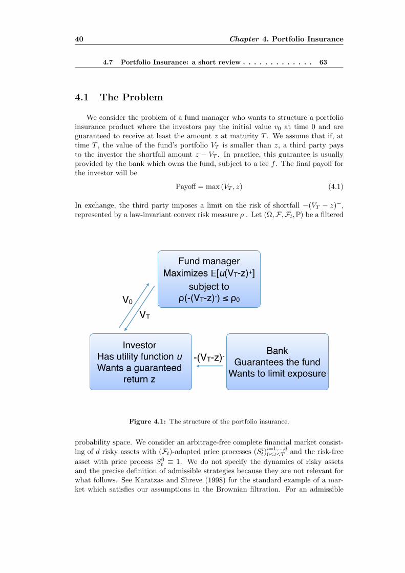
4.1 The Problem
We consider the problem of a fund manager who wants to structure a portfolioinsurance product where the investors pay the initial value v0 at time 0 and areguaranteed to receive at least the amount z at maturity T . We assume that if, attime T , the value of the fund’s portfolio VT is smaller than z, a third party paysto the investor the shortfall amount z − VT . In practice, this guarantee is usuallyprovided by the bank which owns the fund, subject to a fee f . The final payoff forthe investor will be
Payoff = max (VT , z) (4.1)
In exchange, the third party imposes a limit on the risk of shortfall −(VT − z)−,represented by a law-invariant convex risk measure ρ . Let (Ω,F ,Ft,P) be a filtered
BankGuarantees the fund
Wants to limit exposure
InvestorHas utility function uWants a guaranteed
return z
VT
V0
-(VT-z)-
Fund managerMaximizes 𝔼[u(VT-z)+]
subject toρ(-(VT-z)-) ≤ ρ0
Figure 4.1: The structure of the portfolio insurance.
probability space. We consider an arbitrage-free complete financial market consist-ing of d risky assets with (Ft)-adapted price processes (Sit)
i=1,...,d0≤t≤T and the risk-free
asset with price process S0t ≡ 1. We do not specify the dynamics of risky assets
and the precise definition of admissible strategies because they are not relevant forwhat follows. See Karatzas and Shreve (1998) for the standard example of a mar-ket which satisfies our assumptions in the Brownian filtration. For an admissible
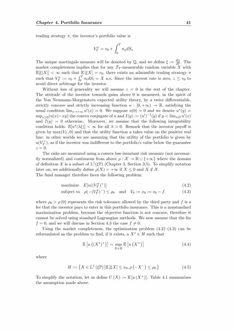
Chapter 4. Portfolio Insurance 41
trading strategy π, the investor’s portfolio value is
V πT = v0 +
∫ T
0πudSu
The unique martingale measure will be denoted by Q, and we define ξ := dQdP . The
market completeness implies that for any FT -measurable random variable X withE[ξ|X|] < ∞ such that E [ξX] = v0, there exists an admissible trading strategy π
such that V πT := v0 +
∫ T0 πtdSt = X a.s. Since the interest rate is zero, z ≤ v0 to
avoid direct arbitrage for the investor.
Without loss of generality we will assume z = 0 in the rest of the chapter.The attitude of the investor towards gains above 0 is measured, in the spirit ofthe Von Neumann-Morgenstern expected utility theory, by a twice differentiable,strictly concave and strictly increasing function u : [0,+∞) → R, satisfying theusual condition limx→+∞ u
′(x) = 0. We suppose u(0) = 0 and we denote u?(y) =supx≥0(u(x)−xy) the convex conjugate of u and I(y) := (u′)−1(y) if y < limx↓0 u
′(x)and I(y) = 0 otherwise. Moreover, we assume that the following integrabilitycondition holds: E[u?(λξ)] < ∞ for all λ > 0. Remark that the investor payoff isgiven by max(VT , 0) and that the utility function u takes value on the positive realline: in other worlds we are assuming that the utility of the portfolio is given byu(V +
T ), as if the investor was indifferent to the portfolio’s value below the guaranteez = 0.
The risks are measured using a convex law-invariant risk measure (not necessar-ily normalized) and continuous from above ρ : X → R ∪ +∞ where the domainof definition X is a subset of L1(ξP) (Chapter 3, Section 3.5). To simplify notationlater on, we additionally define ρ(X) = +∞ if X ≤ 0 and X /∈ X .
The fund manager therefore faces the following problem:
maximize E[u((V πT )+)] (4.2)
subject to ρ(−(V πT )−) ≤ ρ0 and V0 := x0 := v0 − f. (4.3)
where ρ0 > ρ (0) represents the risk tolerance allowed by the third party and f is afee that the investor pays to enter in this portfolio insurance. This is a nonstandardmaximization problem, because the objective function is not concave, therefore itcannot be solved using standard Lagrangian methods. We now assume that the feef = 0, and we will discuss in Section 4.3 the case f 6= 0.
Using the market completeness, the optimization problem (4.2)–(4.3) can bereformulated as the problem to find, if it exists, a X∗ ∈ H such that
E[u((X∗)+
)]= sup
X∈HE[u(X+)]
(4.4)
where
H :=X ∈ L1 (ξP)
∣∣E [ξX] ≤ x0, ρ(−X−
)≤ ρ0
(4.5)
To simplify the notation, let us define U (X) := E [u (X+)]. Table 4.1 summarizesthe assumption made above.
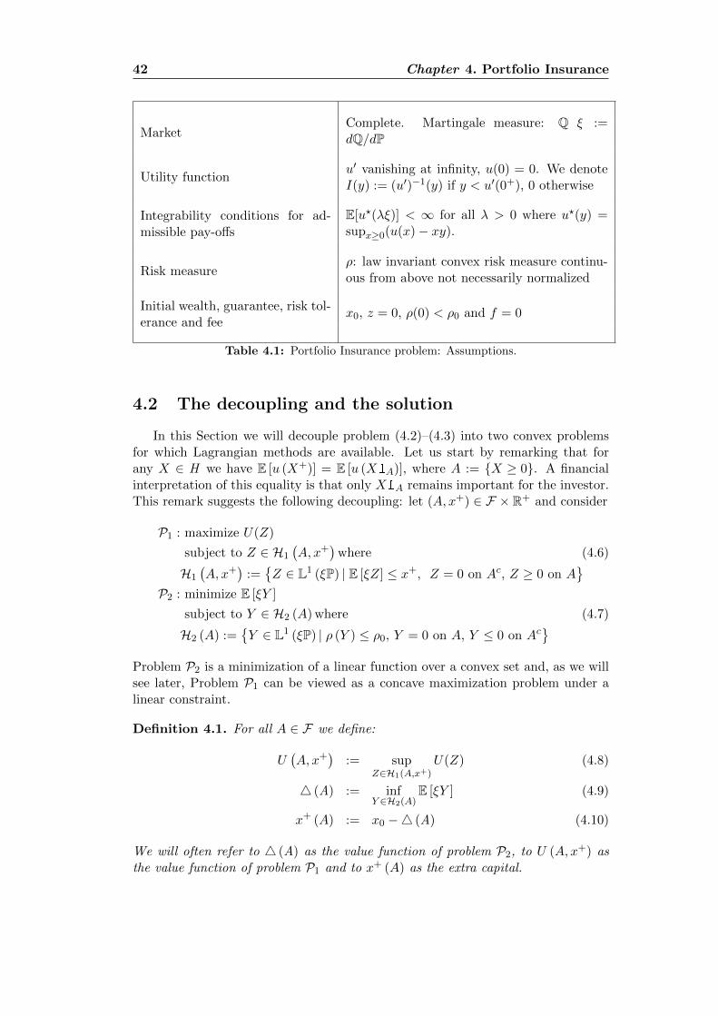
42 Chapter 4. Portfolio Insurance
MarketComplete. Martingale measure: Q ξ :=dQ/dP
Utility functionu′ vanishing at infinity, u(0) = 0. We denoteI(y) := (u′)−1(y) if y < u′(0+), 0 otherwise
Integrability conditions for ad-missible pay-offs
E[u?(λξ)] < ∞ for all λ > 0 where u?(y) =supx≥0(u(x)− xy).
Risk measureρ: law invariant convex risk measure continu-ous from above not necessarily normalized
Initial wealth, guarantee, risk tol-erance and fee
x0, z = 0, ρ(0) < ρ0 and f = 0
Table 4.1: Portfolio Insurance problem: Assumptions.
4.2 The decoupling and the solution
In this Section we will decouple problem (4.2)–(4.3) into two convex problemsfor which Lagrangian methods are available. Let us start by remarking that forany X ∈ H we have E [u (X+)] = E [u (X1A)], where A := X ≥ 0. A financialinterpretation of this equality is that only X1A remains important for the investor.This remark suggests the following decoupling: let (A, x+) ∈ F × R+ and consider
P1 : maximize U(Z)
subject to Z ∈ H1
(A, x+
)where (4.6)
H1
(A, x+
):=Z ∈ L1 (ξP) | E [ξZ] ≤ x+, Z = 0 on Ac, Z ≥ 0 on A
P2 : minimize E [ξY ]
subject to Y ∈ H2 (A) where (4.7)
H2 (A) :=Y ∈ L1 (ξP) | ρ (Y ) ≤ ρ0, Y = 0 on A, Y ≤ 0 on Ac
Problem P2 is a minimization of a linear function over a convex set and, as we willsee later, Problem P1 can be viewed as a concave maximization problem under alinear constraint.
Definition 4.1. For all A ∈ F we define:
U(A, x+
):= sup
Z∈H1(A,x+)
U(Z) (4.8)
4 (A) := infY ∈H2(A)
E [ξY ] (4.9)
x+ (A) := x0 −4 (A) (4.10)
We will often refer to 4 (A) as the value function of problem P2, to U (A, x+) asthe value function of problem P1 and to x+ (A) as the extra capital.
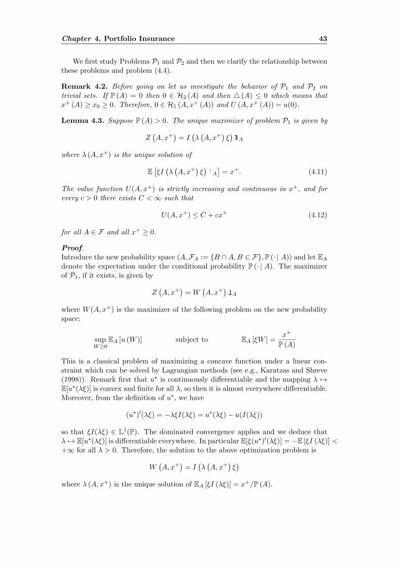
Chapter 4. Portfolio Insurance 43
We first study Problems P1 and P2 and then we clarify the relationship betweenthese problems and problem (4.4).
Remark 4.2. Before going on let us investigate the behavior of P1 and P2 ontrivial sets. If P (A) = 0 then 0 ∈ H2 (A) and then 4 (A) ≤ 0 which means thatx+ (A) ≥ x0 ≥ 0. Therefore, 0 ∈ H1 (A, x+ (A)) and U (A, x+ (A)) = u(0).
Lemma 4.3. Suppose P (A) > 0. The unique maximizer of problem P1 is given by
Z(A, x+
)= I
(λ(A, x+
)ξ)1A
where λ (A, x+) is the unique solution of
E[ξI(λ(A, x+
)ξ)1A
]= x+. (4.11)
The value function U(A, x+) is strictly increasing and continuous in x+, and forevery c > 0 there exists C <∞ such that
U(A, x+) ≤ C + cx+ (4.12)
for all A ∈ F and all x+ ≥ 0.
Proof.Introduce the new probability space (A,FA := B ∩A,B ∈ F,P (· | A)) and let EAdenote the expectation under the conditional probability P (· | A). The maximizerof P1, if it exists, is given by
Z(A, x+
)= W
(A, x+
)1A
where W (A, x+) is the maximizer of the following problem on the new probabilityspace:
supW≥0
EA [u (W )] subject to EA [ξW ] =x+
P (A)
This is a classical problem of maximizing a concave function under a linear con-straint which can be solved by Lagrangian methods (see e.g., Karatzas and Shreve(1998)). Remark first that u? is continuously differentiable and the mapping λ 7→E[u?(λξ)] is convex and finite for all λ, so then it is almost everywhere differentiable.Moreover, from the definition of u∗, we have
(u∗)′(λξ) = −λξI(λξ) = u∗(λξ)− u(I(λξ))
so that ξI(λξ) ∈ L1(P). The dominated convergence applies and we deduce thatλ 7→ E[u?(λξ)] is differentiable everywhere. In particular E[ξ(u?)′(λξ)] = −E [ξI (λξ)] <+∞ for all λ > 0. Therefore, the solution to the above optimization problem is
W(A, x+
)= I
(λ(A, x+
)ξ)
where λ (A, x+) is the unique solution of EA [ξI (λξ)] = x+/P (A).
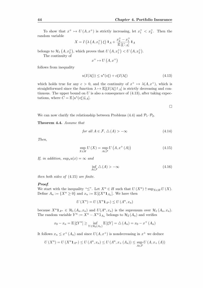
44 Chapter 4. Portfolio Insurance
To show that x+ 7→ U (A, x+) is strictly increasing, let x+1 < x+
2 . Then therandom variable
X = I(λ(A, x+
1
)ξ)1A +
x+2 − x
+1
E [ξ1A]1A
belongs to H1
(A, x+
2
), which proves that U
(A, x+
1
)< U
(A, x+
2
).
The continuity ofx+ 7→ U
(A, x+
)follows from inequality
u(I(λξ)) ≤ u?(cξ) + cξI(λξ) (4.13)
which holds true for any c > 0, and the continuity of x+ 7→ λ(A, x+), which isstraightforward since the function λ 7→ E[ξI(λξ)1A] is strictly decreasing and con-tinuous. The upper bound on U is also a consequence of (4.13), after taking expec-tations, where C = E [u∗(cξ)1A].
We can now clarify the relationship between Problems (4.4) and P1–P2.
Theorem 4.4. Assume that
for all A ∈ F , 4 (A) > −∞ (4.14)
Then,
supX∈H
U (X) = supA∈F
U(A, x+ (A)
)(4.15)
If, in addition, supxu(x) =∞ and
infA∈F4 (A) > −∞ (4.16)
then both sides of (4.15) are finite.
Proof.We start with the inequality “≤”. Let Xn ∈ H such that U (Xn) ↑ supX∈H U (X).Define An := Xn ≥ 0 and xn := E [ξXn1An ]. We have then
U (Xn) = U (Xn1An) ≤ U (An, xn)
because Xn1An ∈ H1 (An, xn) and U(An, xn) is the supremum over H1 (An, xn).The random variable Y n := Xn −Xn
1An belongs to H2 (An) and verifies
x0 − xn = E [ξY n] ≥ infY ∈H2(An)
E [ξY ] = 4 (An) = x0 − x+ (An)
It follows xn ≤ x+ (An) and since U(A, x+) is nondecreasing in x+ we deduce
U (Xn) = U (Xn1An) ≤ U (An, xn) ≤ U (An, x+ (An)) ≤ supA∈F
U (A, x+ (A))
Chapter 4. Portfolio Insurance 45
Let us prove the inequality “≥”. Select An ∈ F such that
U (An, x+ (An)) ↑ supA∈F
U (A, x+ (A)) := m, when n→ +∞
By the assumption of the Theorem, x+(An) < ∞ for all n. If for fixed ε > 0 wecould find, for all n, Xn ∈ H such that
U(Xn) ≥ U (An, x+ (An))− ε (4.17)
then we are done. If P(An) > 0, by Lemma 4.3 there exists an explicit maximizerof Problem P1, denoted by Z(An, x
+), and recall that U(An, x+) = U(Z(An, x
+))is continuous in x+. Therefore, we can find Yn ∈ H2(An) with E[ξYn] sufficientlyclose to 4(An) so that U(An, x0 − E[ξYn]) ≥ U(An, x
+(An)) − ε. Then Xn :=Z(An, x0 − E[ξYn]) + Yn satisfies (4.17). If P(An) = 0 then, as we saw in Remark4.2, taking 0 ∈ H and Xn = 0 satisfies U(Xn) = u(0) = U (An, x+ (An)).
Finally, the fact that m <∞ under Assumption (4.16) follows directly from theestimate (4.12).
Clearly, (4.14) depends on the particular choice of ρ and ξ. In particular, a choiceunder which 4 (A) = −∞ for some A is not appropriate in this kind of portfolioinsurance. As we will see later on an example, the use of the CVaRλ in the Blackand Scholes model yields4 (A) = −∞, whereas the same risk measure coupled witha bounded ξ satisfies (4.16). A simple example clarifies why assumption (4.14) isfundamental in this kind of portfolio insurance:
Example 4.5. Assume that supx u(x) = +∞ anc fix A ∈ F with P (A) > 0 and4 (A) = −∞. It is then possible to find, for each n ∈ N a random variable Y n ∈H2 (A) such that E [ξY n] ≤ −n. Define now
Xn =x0 + n
E [ξ1A]1A + Y n
It is clear that Xn ∈ H for all n and U (Xn) → supx u (x) = +∞, which meansthat Problem (4.4) does not admit a maximizer.
Nevertheless, in practice, it may be difficult to check whenever Assumptions(4.14)–(4.16) hold true: the following proposition, which is simpler to verify, guar-antees them but it is not necessary.
Proposition 4.6. Assume that
γmin (ξP) < +∞, (4.18)
where γmin is the minimal penalty function of ρ defined in (3.2). Then the condition(4.16) holds true.
46 Chapter 4. Portfolio Insurance
Proof.By definition of γmin in (3.2) and the acceptance set related to ρ in (3.1) we have,
γmin (ξP) = supY ∈Aρ
E [−ξY ]
=− ρ0 + sup E [−ξY ] | Y + ρ0 ∈ Aρ≥ − ρ0 + sup E [−ξY ] | Y + ρ0 ∈ Aρ, Y ≤ 0≥ − ρ0 + sup E [−ξY ] | Y + ρ0 ∈ Aρ, Y ≤ 0, Y = 0 on A=− ρ0 −4 (A)
from which the result follows.
Theorem 4.4 gives us a condition under which the value function of problem (4.4)is finite and a way to compute it:
Algorithm 4.7.
1. fix A ∈ F
2. solve P2 (A) and find 4 (A)
3. solve P1 (A) with parameter (A, x+ (A))
4. maximize the value function of problem P1 U (A, x+ (A)) over A ∈ F
The next result establishes a relationship between the maximizers of problem (4.4)and P1–P2.
Theorem 4.8. Let (4.14) hold true.If X∗ achieves the maximum in Problem (4.4) and A∗ := X∗ ≥ 0 then
• A∗ achieves the maximum in the right-hand side of (4.15)
• Y ∗ := X∗ −X∗1A∗ ∈ H2 (A∗) achieves the minimum in P2.
Conversely, let A∗ ∈ F , P (A∗) > 0 and Y ∗ ∈ H2 (A∗) such that
U(A∗, x+ (A∗)
)= supA∈F
U(A, x+ (A)
)E [ξY ∗] =4 (A∗) = inf
Y ∈H2(A∗)E [ξY ]
Then a solution of problem (4.4) is given by
X∗ := I (λ∗ξ)1A∗ + Y ∗ (4.19)
where λ∗ = λ (A∗, x+ (A∗)) verifies (4.11). In this case, the payoff for the investorwill be
Payoff = I (λ∗ξ)1A∗ (4.20)
Chapter 4. Portfolio Insurance 47
Proof.Let X∗ ∈ H be an optimal solution for (4.4), A∗ = X∗ ≥ 0 and Y ∗ = X∗1X∗<0.It is clear that Y ∗ ∈ H2 (A∗). It is also clear that P(A) > 0, since otherwiseE[ξX∗] < x0 which of course is not optimal. Theorem 4.4 and the fact that U(A, x+)is increasing in x+ (Lemma 4.3) give:
supA∈F
U(A, x+ (A)
)= supX∈H
U (X) = U (X∗) = U (X∗1A∗)
=U (A∗, x0 − E[ξY ∗]) ≤ U(A∗, x+ (A∗)
)which means that A∗ achieves the supremum in (4.15). Since U(A, x+) is strictlyincreasing in x+, we shall have x+(A∗) = x0−E[ξY ∗], otherwise we would obtain astrict inequality in the second line of the above estimate, which, of course, yields acontradiction. It follows then that Y ∗ achieves the minimum in P2.
Conversely, assume that A∗ is a maximizer of (4.15) and Y ∗ is a minimizer ofP2. We can then solve Problem P1 with parameters (A∗, x0−4(A∗)) and we know,
by Lemma 4.3, that its solution is given by[I (λ∗ξ)+]+
1A∗ . Let then
X∗ := I (λ∗ξ)1A∗ + Y ∗
We have ρ (−(X∗)−) = ρ (Y ∗) ≤ ρ0 and E [ξX∗] ≤ x0, i.e. X∗ ∈ H . Using Theorem4.4, we conclude our proof:
U (X∗) =U (X∗1A∗) = U(A∗, x+ (A∗)
)= sup
A∈FU(A, x+ (A)
)= sup
X∈HU (X) .
Remark 4.9. Algorithm 4.7 and Theorem 4.4 give us a way to find an optimalsolution for problem (4.4) if we are able to find a maximizer in (4.15) and theminimizer in P2.
But what happens in the case when the maximizer in (4.15) or the minimizerin P2 do not exist? In this case, under Assumption 4.14, following the steps of theproof of Theorem 4.4, one can show that for all ε > 0 there exist Aε ∈ F , λε ∈ Rand Y ε ∈ H2(Aε) such that
Xε := [I (λεξ)]1Aε + Y ε (4.21)
verifies U (Xε) + ε > supX∈H U (X), i.e. Xε is a sequence of ε-optimal solutions.
The main difficulty to apply Theorems 4.4–4.8 is to find a maximizer A∗. Gen-erally, maximization of a set-valued function over F is not simple. Our aim nowis to show that this latter maximization may be carried out over a subset of F ,parameterized by a real number. A similar approach was used in Jin and Yu Zhou(2008), where they faced the same difficulty.
Theorem 4.4 tells us that under Assumption (4.14) we have
supX∈H
U (X) = supA∈F
U(A, x+ (A)
)= sup
A∈Fsup
X∈H1(A,x+(A))
U (X)
48 Chapter 4. Portfolio Insurance
In order to focus our attention on the set dependence, we will introduce the followingnotation:
v (A) := supX∈H1(A,x+(A))
U (X) (4.22)
Let us also define ξ := essinf ξ and ξ := esssup ξ.
Theorem 4.10. Suppose that the law of ξ has no atom and that Assumption (4.14)holds true. Let A ∈ F and c ∈
[ξ, ξ]
such that P (ξ ≤ c) = P (A). Then
v (A) ≤ v(c), where v(c) := v (ξ ≤ c) (4.23)
which means that
supX∈H
U (X) = supA∈F
v (A) = supc∈[ξ,ξ]
v(c). (4.24)
Proof.We will use the methods developed in Jin and Yu Zhou (2008) (see the proof ofTheorem 5.1 therein). There are however some important differences in our proofwhich are due to the presence of a risk measures in our context.
The theorem will be proved in two steps: in Step 1 we will prove that for everyA ∈ F , there exists c ≥ 0 such that 4 (A) ≥ 4 (c) := 4 (ξ ≤ c) so that x+ (c) :=x0 − 4 (ξ ≤ c) ≥ x+ (A), and in Step 2 we will find, for every X ∈ H1 (A, x+)some X ∈ H1 (ξ ≤ c , x+ (c)) such that U(X) ≥ U (X). We conclude then thatv (c) ≥ v (A)
If P(A) = 1 then the result trivially holds true, whereas if P(A) = 0 we can useRemark 4.2 and again the result holds true. Assume then 0 < P (A) < 1 and defineα = P(Ac) = 1− P(A). Let us fix c ∈
[ξ, ξ]
so that
P (ξ ≤ c) = 1− α
This is possible since ξ has no atom. Consider the following sets:
A1 = ξ ≤ c ∩A A2 = ξ > c ∩A (4.25)
B1 = ξ ≤ c ∩Ac B2 = ξ > c ∩Ac (4.26)
Since P(A1)+P(A2) = P(A1)+P(B1) = 1−α it follows P(A2) = P(B1). If P (A2) = 0then A = ξ ≤ c and the result trivially holds true. We can suppose P(A2) > 0.Step 1. Let Y ∈ H2(A). Our aim is to construct Y ∈ H2(ξ ≤ c) with E[ξY ] =E[ξY ] and ρ(Y ) ≥ ρ(Y ). This will imply that 4 (A) ≥ 4(c) since we can decreaseY . Introduce the following notation:
1. f1 (t) := P (Y ≤ t | B1)
2. g1 (t) := P (ξ ≤ t | A2)
3. Z1 = g1 (ξ), that is, L (Z1 | A2) = U([0, 1]), because ξ has no atom.
4. W1 = f−11 (Z1), that is, the law of W1 on A2 is the same as the law of Y on
B1.
Chapter 4. Portfolio Insurance 49
Let
k1 :=
1 if W1 = 0 on A2
E[ξY 1B1 ]E[ξW11A2 ]
otherwise
Observe that since ξ ≤ c on B1, and ξ > c on A2, we have that k ≤ 1. Now define
Y = Y 1B2 + kW11A2 .
By definition, Y = 0 on ξ ≤ c and Y ≤ 0 on ξ ≤ c. In addition, since k1 ≤ 1,we easily get that P(−Y > t) ≤ P(−Y > t) for every t > 0:
P(−Y > t) =P(B2)P(−Y > t | B2) + P(A2)P(−Y > t | A2)
=P(B2)P(−Y > t | B2) + P(B1)P(−kW1 > t | A2)
≥P(B2)P(−Y > t | B2) + P(B1)P(−W1 > t | A2) since k1 ≤ 1
=P(B2)P(−Y > t | B2) + P(B1)P(−Y > t | B1)
=P(−Y > t)
Let F and F be the distribution functions of, respectively, −Y and −Y , and F−1
and F−1 their generalized inverses (defined in (3.4)). From the above inequal-ity, they satisfy F−1(u) ≤ F−1(u) for all u ∈ [0, 1]. Let U be a random vari-able with uniform distribution on [0, 1]. Since ρ is law invariant, we obtain thatρ(Y ) = ρ(−F−1(U)) ≤ ρ(−F−1(U)) = ρ(Y ) ≤ ρ0 and therefore Y ∈ H2(ξ ≤ c).On the other hand, E[ξY ] = E[ξY ] (this is due to our choice of the constant k).Since the choice of Y was arbitrary, this means that 4 (A) ≥ 4(c).
Step 2. Let X be feasible for P1 with parameter (A, x+ (A)), and define
1. f2 (t) := P (X ≤ t | A2)
2. g2 (t) := P (ξ ≤ t | B1)
3. Z2 = g2 (ξ)
4. W2 = f−12 (Z2), that is, the law of W2 on B1 is the same as the law of X on
A2.
Let
k2 :=
1 if W2 = 0 on B1E[ξX1A2 ]E[ξW21B1 ]
otherwise
Note that now, k2 ≥ 1. We define a new random variable X by
X := X1A1 + k2W21B1 +x+ (c)− x+ (A)
E[ξ1ξ≤c
] 1ξ≤c
Since E[ξX]
= x+(c) we deduce X ∈ H1 (ξ ≤ c , x+ (c)). Moreover, since k2 ≥ 1,
similar computations as before yield P(X > t
)≥ P (X > t). By definition
U (X) = E[u(X+)]
=
∫ +∞
0P(X+ > u−1 (t)
)dt
50 Chapter 4. Portfolio Insurance
and since u−1 (t) is positive,X+ > u−1 (t)
=X > u−1 (t)
we conclude that U (X) ≤ U
(X)
.
Theorem 4.10 allows us to simplify Algorithm 4.7:
Algorithm 4.11.
1. fix c ∈[ξ, ξ]
and consider A = ξ ≤ c
2. solve P2 with parameter (ξ ≤ c) and find 4 (c) := 4 (ξ ≤ c)
3. solve P1 with parameters (ξ ≤ c , x+(c)), x+(c) := x0 −4 (c)
4. find c∗, if it exists, that maximizes c→ v (c)
The question of the existence of c∗ which maximizes c → v(c), and the relatedquestion of the existence of the optimal pay-off for the fund manager is difficult toanswer for general risk measures. A complete answer to this question will be givenin Section 4.4 in the case of the entropic risk measure (see Theorem 4.12) and inSection 4.5 for spectral risk measures (Theorem 4.16).
4.3 The fee
The question of the role and the amount of the fee f , which the investor paysto the bank to enter the portfolio insurance scheme, is closely related to the moregeneral issue of the economic rationality of the three-party structure bank—fund—investor. From the point of view of the bank, providing the guarantee is equivalentto providing a put option written on the optimal contingent claim with pay-off(−X∗)+ to the investor (we still suppose z = 0), in exchange of the initial fee f .This transfer of risk from the investor towards the bank makes sense because thebank, as a large financial institution, can accommodate greater losses than the othertwo parties. It is less risk averse than the fund or the investor, and may even berisk seeking. While the fee leads to an immediate return for the bank, the tail riskassociated to the put option may be reduced by diversification, or it may simply bekept on the balance sheet as an unhedgeable risk. These and similar considerationscan induce a bank to provide the portfolio guarantee for a fee which is less thanthe replication price of the put option. On the other hand, the fee cannot begreater than the replication price, since in that case it would be optimal for thefund manager to replicate the guarantee himself, which is not what is observed inreality.
This leads us to a new formulation where the fee is assumed to be a percentageof the no-arbitrage price of the put option:
maximize E[u((VT )+)] (4.27)
over vT subject to
ρ(−(VT )−) ≤ ρ0 and V0 = x0 − pEQ [(−VT )+]. (4.28)
Chapter 4. Portfolio Insurance 51
for p ∈ [0, 1]. The case p = 1 corresponds to the situation when the fee is equal tothe price of the put option: since the bank can completely hedge away her risk, wededuce that the value function does not depend on ρ0, and therefore on the amountof risk which is being transferred to the bank, so one can take from the beginningρ0 = 0 (no risk transfer). In this case, the problem can be transformed into
maximizeE [u(VT )] over VT ≥ 0 and V0 = x0
If the bank asks a fee which completely covers the price of the option she sells, thenthe fund manager has no reason to take any risk.
From now on let 0 ≤ p < 1. Assume that problem (4.2) has a solution, given by(4.19). Since we know that the optimal solution is of the form
V (c) := X(c)1ξ≤c + Y (c)1ξ>c
for c ∈[ξ, ξ], the price of a put option written on V (c) is −4(c). Hence the problem
(4.27)–(4.28) can be transformed into
maximize E[u(I(λcξ))1ξ≤c] (4.29)
over c ∈[ξ, ξ]
where λc satisfies
EQ [I(λcξ)1ξ≤c] = x0 − (1− p)4(c) (4.30)
If there exists a c∗ which maximizes the above expression and P(ξ > c∗) > 0 thenthe solution of this problem is given by
V ∗T := I(λ(c∗)ξ)1ξ≤c∗ + Y (c∗)1ξ>c∗
where Y (c∗) is the solution of problem P2 with parameter ξ ≤ c∗. The effect ofthe fee on the optimal portfolio will be further analyzed in the specific example ofthe entropic risk measure in Section 4.4.
4.4 Explicit result: the Entropic risk measure
4.4.1 The result
In this section we show how Theorems 4.8 and 4.10 can be used to solve problem(4.27)–(4.28) when one uses the entropic risk measure defined in (3.13):
ρβ (X) := β logE[exp
(− 1
βX
)]where β > 0. From (3.14):
ρβ (X) = supQP, log( dQdP )∈L1(Q)
(EQ [−X]− βEQ
[log
(dQdP
)]).
In particular, γmin (ξP) = βE [ξ log (ξ)] .
52 Chapter 4. Portfolio Insurance
Theorem 4.12. Let ρβ to be the entropic risk measure and assume that the stateprice density ξ has no atom and satisfies ξ log ξ ∈ L1 (P ). Assume also that the feeis a fraction p ∈ [0, 1] of the price of the put option corresponding to the guarantee,as in Section 4.3. Then the optimal claim for the fund manager is given by
V ∗ := I (λ (c∗) ξ)1ξ≤c∗ − β[log
(β
η (c∗)ξ
)]+
1ξ>c∗
where
• λ (c) is the unique solution of E[ξI (λ (c) ξ)1ξ≤c
]= x0 − (1− p)4 (c)
• α (c) := P (ξ > c)
• 4 (c) = −βE[ξ log
(βξη(c) ∨ 1
)]• η (c) is the unique solution of: E
[(βξη(c) ∨ 1
)1ξ>c
]= e
ρ0β + α(c)− 1.
• c∗ attains the supremum of c→ E[u (I (λ (c) ξ))1ξ≤c
]Proof.Remark first that the condition ξ log ξ ∈ L1 (P ) implies that Assumptions (4.16)holds true (Proposition 4.6). The proof is just a simple application of Theorems4.8, 4.10, Lemma 4.3 and Lagrangian methods.
We first need to compute the map c→4(c). Fix c and consider the problem:
minimizeE [ξY ] over ρ (Y ) ≤ ρ0, Y = 0 on A and Y ≤ 0 on Ac
whereA = ξ ≤ c. Working on the new space(Ac, F := B ∩Ac, B ∈ F, P := P(·|Ac)
),
we can transform this minimization into
minimize α (c) E [ξW ] over E[exp
(−Wβ
)]≤ δ(c), W ≤ 0
δ (c) =eρ0β + α (c)− 1
α (c)
where E is the expectation under the new probability P and W is a random variableon the new space. Using Lagrangian methods we can find the unique optimalsolution:
W ∗ (c) := −β[log
(β
η (c)ξ
)]+
where η (c) is the unique solution of:
E[(
βξ
η(c)∨ 1
)1ξ>c
]= e
ρ0β + α(c)− 1
so then
Y ∗ (c) := W ∗ (c)1ξ>c.
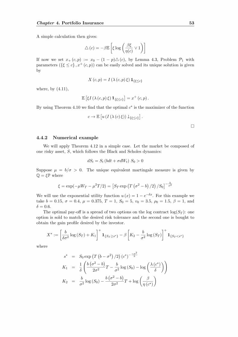
Chapter 4. Portfolio Insurance 53
A simple calculation then gives:
4 (c) = −βE[ξ log
(βξ
η(c)∨ 1
)]If now we set x+ (c, p) := x0 − (1 − p)4 (c), by Lemma 4.3, Problem P1 withparameters (ξ ≤ c , x+ (c, p)) can be easily solved and its unique solution is givenby
X (c, p) = I (λ (c, p) ξ)1ξ≤c
where, by (4.11),
E[ξI (λ (c, p) ξ)1ξ≤c
]= x+ (c, p) .
By using Theorem 4.10 we find that the optimal c∗ is the maximizer of the function
c→ E[u (I (λ (c) ξ))1ξ≤c
].
4.4.2 Numerical example
We will apply Theorem 4.12 in a simple case. Let the market be composed ofone risky asset, S, which follows the Black and Scholes dynamics:
dSt = St (bdt+ σdWt) S0 > 0
Suppose µ = b/σ > 0. The unique equivalent martingale measure is given byQ = ξP where
ξ = exp(−µWT − µ2T/2) =[ST exp
(T(σ2 − b
)/2)/S0
]− bσ2
We will use the exponential utility function u (x) = 1− e−δx. For this example wetake b = 0.15, σ = 0.4, µ = 0.375, T = 1, S0 = 5, v0 = 3.5, ρ0 = 1.5, β = 1, andδ = 0.6.
The optimal pay-off is a spread of two options on the log contract log(ST ): oneoption is sold to match the desired risk tolerance and the second one is bought toobtain the gain profile desired by the investor.
X∗ :=
[b
δσ2log (ST ) +K1
]+
1ST≥s∗ − β[K2 −
b
σ2log (ST )
]+
1ST<s∗
where
s∗ = S0 exp(T(b− σ2
)/2)
(c∗)−−σ2b
K1 =1
δ
(b(σ2 − b
)2σ2
T − b
σ2log (S0)− log
(λ (c∗)
δ
))
K2 =b
σ2log (S0)−
b(σ2 − b
)2σ2
T + log
(β
η (c∗)
)
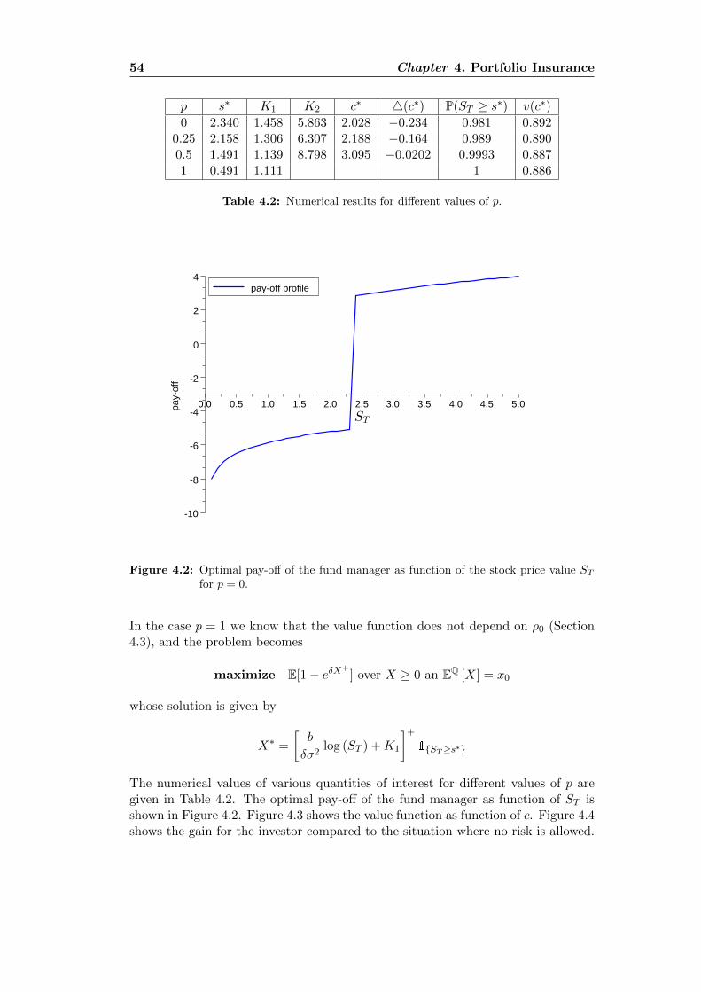
54 Chapter 4. Portfolio Insurance
p s∗ K1 K2 c∗ 4(c∗) P(ST ≥ s∗) v(c∗)
0 2.340 1.458 5.863 2.028 −0.234 0.981 0.8920.25 2.158 1.306 6.307 2.188 −0.164 0.989 0.8900.5 1.491 1.139 8.798 3.095 −0.0202 0.9993 0.8871 0.491 1.111 1 0.886
Table 4.2: Numerical results for different values of p.
pay-off profile
-10
-8
-6
-4
-2
0
2
4
0.0 0.5 1.0 1.5 2.0 2.5 3.0 3.5 4.0 4.5 5.0ST
pay-
off
Figure 4.2: Optimal pay-off of the fund manager as function of the stock price value STfor p = 0.
In the case p = 1 we know that the value function does not depend on ρ0 (Section4.3), and the problem becomes
maximize E[1− eδX+] over X ≥ 0 an EQ [X] = x0
whose solution is given by
X∗ =
[b
δσ2log (ST ) +K1
]+
1ST≥s∗
The numerical values of various quantities of interest for different values of p aregiven in Table 4.2. The optimal pay-off of the fund manager as function of ST isshown in Figure 4.2. Figure 4.3 shows the value function as function of c. Figure 4.4shows the gain for the investor compared to the situation where no risk is allowed.
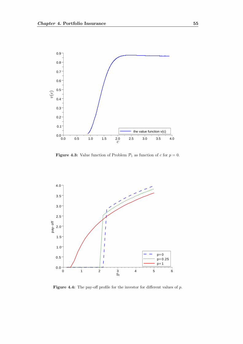
Chapter 4. Portfolio Insurance 55
the value function v(c)0.0
0.1
0.2
0.3
0.4
0.5
0.6
0.7
0.8
0.9
0.0 0.5 1.0 1.5 2.0 2.5 3.0 3.5 4.0c
v(c)
Figure 4.3: Value function of Problem P1 as function of c for p = 0.
p= 0p= 0.25p= 1
0.0
0.5
1.0
1.5
2.0
2.5
3.0
3.5
4.0
0 1 2 3 4 5 6ST
pay
-off
Figure 4.4: The pay-off profile for the investor for different values of p.
56 Chapter 4. Portfolio Insurance
4.5 Explicit result: the spectral risk measure
4.5.1 The result
In this section we solve the portfolio optimization problem (4.27)–(4.28) whenthe risk constraint is given by a spectral risk measure. For a given probability on[0, 1] the related spectral risk measure is given by (3.7)–(3.8) :
ρµ (X) :=
∫ 1
0CV aRβ (X)µ(dβ) or equivalently
ρµ (X) :=
∫ 1
0µ(u)V aRu (X) du where µ(u) :=
∫ 1
u
µ(dx)
x
Following Algorithms 4.7–4.11 we first need to compute the mappings A → 4 (A)and c→4(c):
Lemma 4.13. For A ∈ F with P (A) < 1, let Fξ be the conditional distribution ofξ on Ac and define αA := P (Ac). 4 (A) > −∞ if and only if
limx→0+
F−1ξ (1− x)
µ (x)< +∞ (4.31)
In this case
4 (A) = −ρ0 maxx∈[0,1]
r (x) (4.32)
r (x) :=αA∫ αAx
0 µ (u) du
∫ x
0F−1ξ (1− u) du (4.33)
Proof.In order to compute 4 (A) we reformulate Problem P2 in terms of the conditionaldistribution function of Y ∈ H2 (A) on Ac. Introduce a new probability P viadPdP = 1Ac
αA. Let FY be the distribution function of Y under this probability and F−1
Y
its generalized inverse . Using this new probability we can rewrite the ingredientsof our problem as
E[ξY ] = αAE[ξY ]
and
CV aRβ(Y ) = − 1
β
∫ β
0F−1Y (u) = − 1
β
∫ β∧αA
0F−1Y (u/αA)du
= −αAβ
∫ βαA∧1
0F−1Y (u)du.
Fubini’s theorem gives
ρµ(Y ) = −αA∫ 1
0
∫ 1
010≤αAu≤β∧αAF
−1Y (u)
µ(dβ)
βdu
= −αA∫ 1
0
∫ 1
αAu
µ(dβ)
βF−1Y (u)du
= −αA∫ 1
0µ(αAu)F−1
Y (u)du
To express E[ξY ], we make use of the following Lemma:
Chapter 4. Portfolio Insurance 57
Lemma 4.14. Let F1 and F2 be distribution functions on [0,∞). Then
supX∼F1, Y∼F2
E[XY ] =
∫ 1
0F−1
1 (u)F−12 (u)du.
The proof of this result is given in Paragraph 4.5.2.
We can transform problem P2 as
4 (A) = αA inf
∫ 1
0F−1ξ (u)F−1
Y (1− u)du (4.34)
subject to − αA∫ 1
0µ (αAu) F−1
Y (u)du ≤ ρ0, (4.35)
where the inf is taken over all generalized inverse distribution functions F−1Y of
non-positive random variables. Such a function can always be written as
F−1Y (u) := −
∫ 1
uζ (du) , (4.36)
where ζ is a positive measure on [0, 1]. By using Fubini’s theorem we can rewriteproblem (4.34)–(4.35) in terms of this measure:
4 (A) = −αA sup
(∫ 1
0ζ(ds)
∫ s
0F−1ξ (1− u)du
)subject to αA
(∫ 1
0ζ(ds)
∫ s
0µ (αAu) du
)≤ ρ0.
The solution of this problem can easily be shown to be a point mass: ζ = hδx whereh ≥ 0 and x ∈ [0, 1] can be found from
4 (A) = −αA sup
(h
∫ x
0F−1ξ (1− u)du
)(4.37)
subject to αAh
∫ x
0µ (αAu) du = ρ0, (4.38)
The constraint (4.38) gives us
h = h (x) =ρ0
αA∫ x
0 µ (αAs) ds
and using definition (4.33) we get
4 (A) = −αA supx∈[0,1]
(ρ0
αA∫ x
0 µ (αAs) ds
∫ x
0F−1ξ (1− u)du
)= −ρ0 max
x∈[0,1]r (x)
The function r is differentiable on (0, 1] and may only have a singularity at x = 0;using l’Hopital’s rule, we get
r(0+)
= limx→0
F−1ξ (1− x)
µ (x)
So 4 (A) > −∞ if and only if r is bounded on [0, 1], which is true if and only ifr (0+) < +∞.

58 Chapter 4. Portfolio Insurance
Corollary 4.15. The function 4(c) is given by
4(c) = −ρ0 max0≤z≤α(c)
R(z), R(z) :=E[ξ11−Fξ(ξ)<z
]∫ z
0 µ (u) du
Assume that the limit
limx→0+
F−1ξ (1− x)
µ (x)(4.39)
exists. Then
limc↑ξ4(c) = −ρ0 lim
x→0+
F−1ξ (1− x)
µ (x).
Proof.In order to make the dependence on c explicit, we introduce the notation
4 (c) := −ρ0 maxx∈[0,1]
R (x, c)
where
R (x, c) :=α (c)
∫ x0 F
−1ξ (1− u) du∫ α(c)x
0 µ (u) du
which holds true from Lemma 4.13. Noting that F−1ξ (1− u) = F−1
ξ (1− α(c)u) ≥ cand making a change of variable,
R (x, c) =E[ξ1c<ξ1F−1
ξ (1−x)<ξ]
∫ α(c)x0 µ (u) du
=E[ξ1F−1
ξ (1−α(c)x)<ξ]
∫ α(c)x0 µ (u) du
=E[ξ11−Fξ(ξ)<α(c)x
]∫ α(c)x
0 µ (u) du
The function 4(c) can then be rewritten as
4(c) = −ρ0 max0≤z≤α(c)
R(z), R(z) :=E[ξ11−Fξ(ξ)<z
]∫ z
0 µ (u) du
The following theorem, which is the main result of this section, characterizes thesolution of the problem (4.4) when the risk constraint is given by a spectral riskmeasure via an one-dimensional optimization problem.
Chapter 4. Portfolio Insurance 59
Theorem 4.16. Assume that there exists c∗ with P[ξ > c∗] > 0 such that v(c∗) =maxξ≤c≤ξ v(c) with
v(c) = E[u(I(λ(c)ξ))1ξ≤c],
where λ(c) is the solution of
E[ξI(λ(c)ξ)1ξ≤c] = x0 +ρ0E[ξ1ξ>c]∫ P[ξ>c]
0 µ(u)du.
Then the solution to the problem (4.4) is given by
X∗ = I(λ(c∗)ξ)1ξ≤c∗ −ρ0∫ P[ξ>c∗]
0 µ(u)du1ξ>c∗ .
Proof.From Theorem 4.10 we need to maximize the function c → v(c) over c ∈ [ξ, ξ].Assume that v(c) achieves its maximum at the point c∗ such that 4(c∗) = −ρR(z)with z < α(c) and let c′ = α−1(z). Then 4(c) is constant on the interval [c, c′],which means that x+(c) = x+(c′),
H1
(ξ ≤ c , x+(c)
)⊂ H1
(ξ ≤ c′
, x+(c′)
)and therefore v(c) ≤ v(c′). This argument shows that the solution of the optimiza-tion problem appearing in the right-hand side of (4.24) does not change if we replacethe expression for 4(c) given by Corollary 4.15 by
−ρ0R(α(c)) = −ρ0E[ξ1ξ>c]∫ P[ξ>c]
0 µ(u)du.
Applying Lemma 4.3 we then find
v(c) = E[u(I(λ(c)ξ))1ξ≤c],
where
E[ξI(λ(c)ξ)1ξ≤c] = x0 +ρ0E[ξ1ξ>c]∫ P[ξ>c]
0 µ(u)du.
If there exists a c∗ with P(ξ > c∗) > 0 which maximizes the value function c→ v(c)then the optimal contingent claim is given by
X∗ = I(λ(c∗)ξ)1ξ≤c∗ −ρ0∫ P[ξ>c∗]
0 µ(u)du1ξ>c∗ .
where− ρ0∫ P[ξ>c∗]
0 µ(u)du1ξ>c∗ .
is the optimal solution of Problem P2 corresponding to ξ ≤ c∗, which can bededuced from the proof of Lemma 4.13.
60 Chapter 4. Portfolio Insurance
Remark 4.17. If supξ≤c≤ξ v(c) is attained only by c∗ = ξ and
limc→ξ
E[ξ1ξ>c]∫ P[ξ>c]0 µ(u)du
<∞,
(the latter condition holds, in particular, if ξ < ∞), then infA∈F ∆(A) > −∞but this infimum is not achieved: the extra gain from allowing a risk tolerance isbounded, but the optimal claim does not exist. Intuitively, claims which are “almostoptimal” will lead to a very large loss occurring with a very small probability.
If
lim supc→ξ
E[ξ1ξ>c]∫ P[ξ>c]0 µ(u)du
=∞
then infA∈F 4(A) = −∞: the extra gain from allowing a risk tolerance is un-bounded.
4.5.2 Proof of Lemma 4.14
Proof.It will be easier to work with survival functions F1(x) = 1 − F1(x) and F2(x) =1−F2(x) rather than distribution functions. Let F (x, y) = P(X > x, Y > y) denotethe 2-dimensional survival function of (X,Y ). By Fubini’s theorem and elementarybounds on distribution functions,
E[XY ] =
∫ ∞0
∫ ∞0
F (x, y)dxdy ≤∫ ∞
0
∫ ∞0
min(F1(x), F2(y))dxdy,
which means that the maximum of E[XY ] is attained when the survival function ofX and Y is equal to min(F1(x), F2(y)). But it is straightforward to check that thesurvival function of the couple (F−1
1 (U), F−12 (U)), where U is uniform on [0, 1], has
exactly this form.
4.5.3 The special case: CV aRβ
Definition 3.13 gives that the CV aRβ is a special case of spectral risk measure,when one takes µ (du) = δβ (du), which yields µβ (x) := 1
β1β>x. The condition(4.31) appearing in Lemma 4.13 becomes
limx→0+
βF−1ξ (1− x) = βξ
Corollary 4.15, Lemma 4.3 and Theorems 4.10 and 4.16 enable us to give the solutionof Problem (4.4):
• If ξ := essup ξ <∞, then the value function of problem (4.4) is:
supX∈H
U (X) = supc∈[ξ, ξ]
E[u (I (λ (c) ξ))1ξ≤c
](4.40)
Chapter 4. Portfolio Insurance 61
where λ (c) is the unique solution of
E[ξI (λ (c) ξ)1ξ≤c
]= x0 + ρ0
E[ξ1ξ>c]
1 ∧ α(c)β
• If ξ = +∞ then there exists A ∈ F with 4 (A) = −∞.
The maximum in (4.40) is always attained for some c∗ ∈ [ξ, ξ] because the value
function is continuous and [ξ, ξ] is compact. If c∗ < ξ then Theorem 4.16 appliesand then we have a optimal solution for Problem (4.4). If the maximum is attainedat c∗ = ξ, then, as in Remark 4.17, the optimal claim does not exist.
Remark 4.18. From (3.6), the minimal penalty function for the CV ARβ is givenby:
γmin (Q) :=
0 if dQ
dP ≤1β , P-a.s
+∞ otherwise
If ξ is bounded but P(ξ > 1
β
)> 0 then γmin (ξP) = +∞ and we have an example of
a situation where Assumption (4.16) holds true but the stronger assumption (4.18)does not.
4.6 Explicit result: the G-divergence
The goal of this section is to solve problem (4.4) when ρ is related to someG-divergence. Let then G be a convex, increasing and non constant function, withG(0) = 0, G(1) < +∞ and G(x)/x → +∞ when x → +∞. The risk measurerelated to G was introduced in Section 3.4:
ρG(X) := supQP, IG(Q|P)<+∞
(EQ [−X]− IG(Q | P)
)or equivalently, by (3.12):
ρG(X) := inft∈R
(E [G∗(t−X)]− t)
where G∗(u) := supu>0(ut − G(u)). In order to solve problem (4.4) let us firstcompute the map A→4 (A). For this we introduce, for t ∈ R
4(A, t) := infY ∈H2(A,t)
E [ξY ] where (4.41)
H2(A, t) :=Y ∈ L1(ξP) | E [G∗(t+ Y )] ≤ ρ0 + t, Y = 0 on A, Y ≤ 0 on Ac
Lemma 4.19. Let G : R → R+ ∪ +∞ to be a convex, increasing function withG(0) = 0, G(x)/x → +∞ when x +∞ and assume that there exists some ε > 0such that G(1 + ε) < +∞. Then
4 (A) := inft∈R4(A, t)

62 Chapter 4. Portfolio Insurance
Proof.From the definition of 4 (A) in (4.9) and H2 (A) in (4.7) we have
H2(A, t) ⊆ H2 (A) , for all t ∈ R
which means that 4(A, t) ≥ 4 (A), so then inft4(A, t) ≥ 4 (A). The equalityholds true if we will show that for any Y ∈ H2 (A) there exists a t ∈ R such thatY ∈ H2(A, t). For sake of clarity, let us introduce ψ(t) := E [G∗(t+ Y )] − t. It isstraightforward to prove that ψ is convex. Furthermore for some η ∈ (0, 1) we have
limt→+∞
ψ(t)
t≥ E
[lim inft→+∞
G∗(t+ Y )
t
]− 1
≥ E[lim inft→+∞
((1 + ε)
(1 +
Y
t
)− G(1 + ε)
t
])− 1
≥ ε
limt→−∞
ψ(t)
t≤ E
[lim supt→−∞
G∗(t+ Y )
t
]− 1
≤ E[lim supt→−∞
((1− η)
(1 +
Y
t
)− G(1− η)
t
])− 1
≤ −η
which proves that ψ is a coercive function: for any Y ∈ H2 (A) there exists a tY ∈ Rsuch that
inft∈R
(E [G∗(t+ Y )]− t) = E [G∗(tY + Y )]− tY
so then Y ∈ H2(A, tY ) which concludes our proof.
Remark how both the CV aR and the Entropy satisfy the assumptions of Lemma4.19.
To compute 4(A, t) we can use Lagrangian arguments: on the new space(A, FA := A ∩B|B ∈ F , P := P(|A)
)we can transform the problem into
minimize αAE [ξY ] over Y ≤ 0 and (4.42)
E [G∗(t+ Y )] ≤ ρ0 + t−G∗(t)(1− αA)
αA
where αA := P(A) and E is the expectation under P. Once we know 4(A, t) forall t we first apply Lemma 4.19 and then Algorithm 4.11 gives us a way to solveproblem (4.4).
Chapter 4. Portfolio Insurance 63
4.7 Portfolio Insurance: a short review
Portfolio insurance is a widely popular concept in financial industry, and thereexists an extensive literature on this topic. When the guarantee constraint is im-posed in an almost sure way, a common strategy is the option based portfolio in-surance, which uses put options written on the underlying risky asset as protection.The optimality of OBPI for European and American capital guarantee is studied inEl Karoui et al. (2005). The difficulty of finding a sufficiently long-dated option foruse in OBPI has lead to the appearance of strategies which involve only the under-lying risky asset, of which the most popular is the Constant Proportion PortfolioInsurance (CPPI), (Black and Perold, 1992), where the exposure to the risky assetis proportional to the difference between the value of the fund and the discountedvalue of the guaranteed payment. If the price path of the underlying risky assetadmits jumps, the CPPI strategy no longer ensures that the fund value will be a.s.above the guaranteed level at maturity, unless the portfolio is completely delever-aged (Cont and Tankov, 2009), which usually imposes too strong a restriction onthe potential gains. The current market practice is therefore to require that theportfolio stays above the guaranteed level with a sufficiently high probability, or,for example, that it remains above the guarantee for a certain set of stress scenarios,chosen from historical data coming from highly volatile periods. A more flexibleapproach, which can take into account not only the probability of loss but also thesizes of potential losses, is to impose a constraint on a risk measure of the shortfall.This has led to the development of literature on portfolio insurance and, more gen-erally, portfolio optimization under probabilistic / risk measure constraints.
Emmer et al. (2001) study one-period portfolio optimization under Capital-at-Riskconstraint (the Capital-at-Risk is defined as the difference between the mean valueof the portfolio and its VaR). Still in the one-period setting, Rockafellar and Urya-sev (2000) provide an algorithm for minimizing the CVaR of a portfolio under areturn constraint. Basak and Shapiro (2001) solve the utility optimization prob-lem under the VaR constraint and Boyle and Tian (2007) discuss continuous-timeportfolio optimization under the constraint to outperform a given benchmark witha certain confidence level. Like us, these authors also face some issues related tothe non-convexity of the optimization problem, although the non-convexity appearsfor a different reason (non-convexity of the constraint itself). Another stream ofliterature (Follmer and Leukert, 1999; Bouchard et al., 2009) considers hedgingproblems when the hedging constraint is imposed with a certain confidence levelrather than almost surely. The viscosity solution approach of Bouchard et al. (2009)was extended in (Bouchard et al., 2010) to stochastic control problems under targetconstraint (that is, for example, under the constraint to outperform a benchmarkwith a certain probability) but it does not seem possible to treat risk measure con-straints in this setting. He and Zhou (2010) have recently introduced a generalmethodology for solving law-invariant portfolio optimization problems by reformu-lating them in terms of the quantile function of the terminal value of the portfolio.While such a reformulation is in principle possible for our problem by using thedual representation results for law-invariant convex risk measures (see Follmer andSchied (2004) and Jouini et al. (2006)), the resulting problem is still non-linear and

64 Chapter 4. Portfolio Insurance
non-convex so such a transformation does not necessarily simplify the treatment.Gundel and Weber (2007) solve the problem of maximizing the robust utility of aportfolio under a constraint on the expected shortfall, which includes, in particu-lar, all coherent risk measures. Rogers (2009) discusses utility optimization when aportfolio constraint in the form of a coherent risk measure is present, and goes onto study optimal contracting problems in this context. The main difference/noveltyof our work from these two studies is that in our approach, the utility function isonly applied to positive gains while the risk measure is only applied to negativeshortfall. This brings us much closer to the reality of portfolio insurance and at thesame time allows to obtain explicit solutions.

Part II
Quadratic Hedge
65

Chapter 5
Quadratic hedge: introductionand main properties
The Chapter is organized as follows: we first introduce the Quadratic Hedge prob-lem in its most general formulation and give a review of the literature on the subject.In Section 5.2 we introduce the general model, the value function associated to theQuadratic Hedge problem, we define the so called Pure investment problem and westudy the structure of these value functions (Sections 5.3 and 5.4). Next, with a ver-ification argument, we characterize the value functions of the pure investment andthe quadratic hedge problems as the unique solution of a semi linear partial integro-differential equations (Sections 5.5 and 5.6). We finally do a short digression onthe theory of viscosity solutions and how it can be used in this context (Section 5.7).
Contents
5.1 Introduction . . . . . . . . . . . . . . . . . . . . . . . . . . 675.2 The Model . . . . . . . . . . . . . . . . . . . . . . . . . . . 715.3 The pure investment problem: a priori estimate . . . . . 74
5.3.1 Proof of Lemma 5.5 . . . . . . . . . . . . . . . . . . . . . 825.3.2 Proof of Lemma 5.6 . . . . . . . . . . . . . . . . . . . . . 835.3.3 Proof of Lemma 5.7 . . . . . . . . . . . . . . . . . . . . . 86
5.4 The structure of the quadratic hedge value function . . 895.5 The pure investment problem: verification . . . . . . . . 915.6 The quadratic hedge problem: verification . . . . . . . . 945.7 Viscosity solutions . . . . . . . . . . . . . . . . . . . . . . . 96
5.1 Introduction
In incomplete markets the perfect hedge does not exist in general, and most ofthe markets are incomplete. In these cases, pricing and hedging an option is a hardtask since one cannot totally hedge away the risk. Once we accept that a residual riskmay affect our hedging strategy, an important issue, especially from a practitioner’spoint of view, is to quantify and control this residual risk. A common way tomeasure this residual risk is to compute the expected squared distance between theoption one wants to hedge and the portfolio. The quadratic hedge problem is to
67
68 Chapter 5. Quadratic hedge: introduction and main properties
find the optimal portfolio which minimizes this residual risk. In its most generalform the quadratic hedge problem can be formulated as follows: consider a randomvariable H ∈ L2 (FT ,P) and a set of admissible strategies, which has to be carefullyspecified,
θ ∈ X ⊆ L (S) (5.1)
where S is a semimartingale modeling the stock price. Up to appropriate integra-bility conditions, the quadratic hedge problem becomes
minimize EP
[(x+
∫ T
0θt−dSt −H
)2]
over x ∈ R and θ ∈ X (5.2)
If (x∗, θ∗) achieves this infimum, we call θ∗ the optimal mean-variance hedgingstrategy and x∗ its price. When one defines
A :=
x+
∫ T
0θtdSt | x ∈ R, θ ∈ X
then problem (5.2) can be viewed as the L2-projection of H on the space A: onetries to minimize the L2-distance between the contingent claim H and a set of alladmissible portfolios in A.
The quadratic hedge problem is a particular case of the so called utility-basedpricing and hedging problem: for an utility function U one tries to solve
maximize EP[U
(x+
∫ T
0θtdSt −H
)]over x ∈ R and θ ∈ X
For a complete overview on the utility-based indifference price problem we referto El Karoui and Rouge (2000); Schweizer (2001); Delbaen et al. (2002). Assumenow that (xH , θH) achieves the maximum in the above problem and consider thefollowing map P from L2 to R:
P : L2(FT ,P) 3 H → xH ∈ R
Generally this map is not linear, unless one takes U(x) = −x2, which correspondsto the quadratic hedge problem. Although one cannot speak of pricing rule (theutility function has to be increasing and this is not the case), the fact that the abovemapping P is linear has several advantages: from a practical point of view, whenone wants to price an entire portfolio, let us say H =
∑iHi, according to (5.2), she
can first compute the prices corresponding to the single positions Hi, and then addthem up to obtain the portfolio’s price.
Several methods have been proposed to solve the quadratic hedge problem,depending on the features of the semimartingale S or on the set of admissiblestrategies X . An elegant solution is provided when S is a martingale under thehistorical probability P, by using the Galtchouk-Kunita-Watanabe decomposition(Kunita and Watanabe, 1967; Galtchouk, 1976): since H ∈ L2(P,FT ), one can finda predictable process θH ∈ L(S) such that
H = EP [H] +
∫ T
0θHu−dSu +NH
T a.s.
Chapter 5. Quadratic hedge: introduction and main properties 69
whereNHt := EP
[NHT | FT
]is a square integrable martingale such thatNH
t
∫ t0 θu−dSu
is still a martingale under P, i.e. (NHt )t is strongly orthogonal to the set A. By
using this decomposition it is straightforward to deduce that the problem (5.2) issolved by θ∗ = θH and x∗ = EP [H]. Even if the Galtchouk-Kunita-Watanabe de-composition gives the optimal hedging strategy and the minimal price in problem(5.2), some important questions naturally arise when one wants to compute it inpractice: firstly, does θH belong to X ? and if it is the case, can it be thought as atrading strategy, i.e. is it caglad? In many important cases, the answer is positive,and it is also possible to compute the hedging strategy semi-explicitly, in particularwhen S is Levy process (Cont and Tankov, 2004) or, more generally, if S is a generalMarkov jump martingale (Cont, Tankov, and Voltchkova, 2007).
When S fails to be a martingale under P, problem (5.2) becomes much more dif-ficult because the Galtchouk-Kunita-Watanabe decomposition is no longer available.To solve the quadratic hedge problem many authors have exploited the particularfeatures of the model S which allow to find the solution of problem (5.2), but itis no longer explicit enough (which is an important question since this procedureis commonly used in practice). For example, when S is a continuous Ito process,the solution can be found by making an appropriate change of probability in prob-lem (5.2), and then using the Galtchouk-Kunita-Watanabe decomposition to obtainthe optimal hedging strategy. For a complete review on this procedure we refer toLaurent and Pham (1999) or Pham (2000).
The idea of looking for a suitable change of probability that makes S a martingaleturns out to be the key tool to solve the quadratic hedge problem in a general setting:it can be proved that this suitable martingale measure can be obtained by solvingproblem (5.2) for H = 0 and x = 1:
minimize EP
[(1 +
∫ T
0θtdSt
)2], over θ ∈ X (5.3)
In the literature this problem is known as the pure investment problem. In a generalsetting (i.e. S discontinuous semimartingale ) Cerny and Kallsen (2007) give manyinteresting properties of problem (5.3) and provide its solution. They derive thenthe optimal strategy of problem (5.2) and, in particular, they find that it is givenby:
θ∗t = αt−Xθ∗t− + βt,−, Xθ∗
t = x+
∫ t
0θ∗r−dSr
for some semi-explicit processes α, β, where α does not depend on the particularoption H and it is related to the optimal solution of problem (5.3), whereas β lin-early depends on H. This procedure completely characterizes the optimal hedgingstrategy in problem (5.2) but, nevertheless, this solution is no longer explicit for alltypes of semimartingale S, unless the stock price S has a particular structure: withstationary and independent increment (Hubalek, Kallsen, and Krawczyk, 2006) oraffine stochastic volatility models (Cerny and Kallsen, 2008; Kallsen and Vierthauer,2009).
Our contribution is to give a systematic way to solve problem (5.2) when S is ageneral Markov jump process but not necessarily a P-martingale by using stochastic
70 Chapter 5. Quadratic hedge: introduction and main properties
optimization tools (value function and Hamilton-Jacobi-Bellman equation). All overthe work, we tried to move according to the following objectives:
• Considering a sufficiently general model which allows us to apply our resultsto some practical problems (which partially motivated our work)
• Solving problem (5.2) and characterizing the optimal hedging strategy in themore explicit way
• Proving regularity, in a sense which has to be specified, of the optimal hedgingstrategy
As we will explain in Chapter 8, portfolio management in electricity marketsmotivated our work. We think it is helpful to briefly anticipate the main lines ofthat Chapter in order to understand our model on S.The electricity spot price is generally modeled by a Levy-driven process whereas atypical hedging instrument available in this market (the semimartingale S) is thefuture contract, which turns out to be Markov jump process and it does not possesthe martingale property under P. Moreover the spot price process may affect thedynamics of the future contract price, and since the electricity cannot be stored,one has to consider it as a non hedgeable source of risk like, for example, a volatilityfactor. We concentrate on European options written on S which may also dependon the spot price at maturity and on some other non hedgeable source of risk like,for example, the temperature.
The price of our hedging instrument is denoted by S = exp(Z), U denotes thespot price process and P the temperature, where (Z,U, P ) is a R3-valued Markovjump process. The quadratic hedge problem for practitioners of the electricitymarkets can be formulated as follows
minimize E
[(H(UT , PT , e
ZT )− x−∫ T
0θr−de
Zr
)2]
(5.4)
over x ∈ R, θ ∈ X
Problem (5.4) can be also viewed as a constrained quadratic hedge problem: ifS := (S,U, P ) then the problem above can be rewritten as
minimize E
[(H(ST )− x−
∫ T
0θ′r−dSr
)2]
over x ∈ R and θ ∈ L(S), θ2 = θ3 = 0
In order to solve problem (5.4) with the classical instruments of the stochasticoptimization, we will assume that the dynamics of the state variable are of Markovtype with appropriate assumptions on their coefficients. This will allow us to writeand solve the partial integro-differential equation (PIDE) associated to the aboveproblem in a particular space of smooth functions. A particular attention will bedevoted to the case H = 0 since, as we have seen, this is a fundamental tool to solvethe quadratic hedge problem.Still inspired by practical problems, we will consider essentially three different cases:when Z is a jump-diffusion process (Chapter 6) and when it is a pure jump processwith infinite/finite variation (Chapter 7). The pure jump case is quite interesting
Chapter 5. Quadratic hedge: introduction and main properties 71
since, in commodities markets, upward and downward movements of the stock priceprocess S (and then Z) are essentially due to jumps. To conclude, we want to pointout that our goal is proving that the value function of problem (5.4) is smooth(so that the optimal strategy also is): this is important from a numerical pointof view and also because it will give us a better understanding of the optimalstrategy behavior (their derivatives), which is undoubtedly an important task inrisk management.
5.2 The Model
Let (Ω,F ,Ft,P) be a filtered probability space. On this space we introducetwo independent Brownian motions W and B, taking values respectively in R2
and R, and two independent Poisson random measures J and N on R \ 0, bothindependent from W and B. We assume that Ft is the natural filtration of J, N ,W and B and that F0 is augmented with the null sets. We also assume F = FTwhere T > 0 is given. Furthermore
[W 1, W 2
]t
= λt for some λ ∈ (−1, 1). Thepositive Levy measure on R \ 0 related to J is denoted by ν (dy) and it satisfiesthe standard integrability condition
∫R(1 ∧ |y|2
)ν (dy) < ∞. The same holds true
for the Levy measure νn(dy) associated to N . We denote
J(dydt) = J(dydt)− ν(dy)dt N(dydt) = N(dydt)− νn(dy)dt
the compensated Poisson measures on R and
J(dydt) :=J(dydt)− dt× ν(dy)1|y|≤1, N(dydt) :=N(dydt)− dt× νn(dy)1|y|≤1
On this probability space we introduce the family of R3-valued Markov jump pro-cesses (Z,U, P ) as follows:
dZt,u,zr :=µ(r, U t,ur , Zt,u,zr
)dr + σ(r, U t,ur , Zt,u,zr )dW 1
r +
∫Rγ(r, U t,ur− , Z
t,u,zr− , y
)J (dydr)
dU t,ur :=µU (r, U t,ur )dr + σU (r, U t,ur )dBr +
∫RγU(r, U t,ur− , y
)N (dydr)
dP t,pr :=µP (r, P t,pr )dr + σP (r, P t,pr )dW 2r +
∫RγP (r, P t,pr , y)J (dydr) (5.5)
with initial conditions Zt,u,zt = z, U t,ut = u and P t,pt = p, for t ∈ [0, T ) and z, u, p ∈R. The stock price process S is given by S = exp(Z).
We make the following assumptions:
Assumption 5.1.[C]- The coefficients-1.
i). There exists µ ≥ 0 such that max(‖µ‖∞ ,
∥∥µU∥∥∞ , ∥∥µP∥∥∞) ≤ µ.
ii). The volatility functions σ, σU , σP take values in [σmin, σmax], for some 0 ≤σmin ≤ σmax.
iii). For all t ∈ [0, T ] and u, y ∈ R the functions z → µ(t, u, z), z → σ(t, u, z) andz → γ(t, u, z, y) belong to C1(R).
72 Chapter 5. Quadratic hedge: introduction and main properties
iv). There exist two constants Kclip ≥ 0, Kd
lip ≥ 0 and a positive locally bounded
function ρ : R→ R+ such that for all y ∈ R we have∣∣µ(t, u, z)− µ(t, u′, z′)∣∣ ≤ Kc
lip
(|z − z′|+ |u− u′|
)∣∣σ(t, u, z)− σ(t, u′, z′)∣∣ ≤ Kc
lip
(|z − z′|+ |u− u′|
)∣∣γ(t, u, z, y)− γ(t, u′, z′, y)∣∣ ≤ Kd
lipρ(y)(|z − z′|+ |u− u′|
)for all t ∈ [0, T ], z, z′, u, u′ ∈ R.
v). Property iv) holds true for µU , σU and γU (resp. µP , σP and γP ) for somepositive constant KU ≥ 0 and some positive locally bounded function ρU (resp.some KP ≥ 0 and some positive locally bounded function ρP )
[I1]- Integrability conditions-1. The functions
τ (y) := max
(supt,u,z
(|γ (t, u, z, y) |,
∣∣∣eγ(t,u,z,y) − 1∣∣∣) , ρ(y)
)τU (y) := max
(supt,u|γU (t, u, y)|, ρU (y)
)τP (y) := max
(supt,p|γP (t, p, y)|, ρP (y)
)verify τ, τP ∈ L2(R, ν(dy)) and τU ∈ L2(R, νn(dy)).
[I2]- Integrability conditions-2. The function τ verifies τ ∈ L4(|y[≥ 1, ν(dy)).
We define Kmax := max(Kclip, K
dlip),
µ :=µ+1
2σ2 +
∫|y|<1
(eγ − 1− γ)ν(dy) and ‖µ‖ := supt,u,z|µ(t, u, z)| (5.6)
and
|Γ| :=∫R
Γ(y)ν(dy), where Γ(y) := inft,u,z
(eγ(t,u,z,y) − 1
)2(5.7)
In the rest of the chapter we denote ‖τ‖1,ν :=∫|y|≥1 τ(y)ν(dy) whereas ‖τ‖22,ν :=∫
R τ2(y)ν(dy). The same convention holds for τP and τU (with respect to the Levy
measure νn(dy)).
It is well known that there exists a unique semimartingale (U,Z, P ) which solvesthe SDE (5.5) (see for example Jacod and Shiryaev (2003) or Protter (2004)).
Let us introduce the set of admissible strategies θ in problem (5.4): as alreadypointed out in Cerny and Kallsen (2007), this set has to be carefully chosen: if itis too wide we may violate the principle of no arbitrage; if it is too small we may
Chapter 5. Quadratic hedge: introduction and main properties 73
not be able to find the optimal strategies. We follow Cerny and Kallsen (2007) todefine a good set of admissible strategies: first let us introduce the sets of simplecaglad strategies:
D :=
θ := Y0 +
∑i
Yi1]ςi,ςi+1], Yi ∈ L∞(Fςi) and ςi ≤ ςi+1 are stopping times
Dt :=
θ1(t,T ] | θ ∈ D
(5.8)
Dt denotes the L2(P)-closure of Dt, and for t, u, z, x ∈ [0, T )×R3, θ ∈ Dt we definethe wealth process as
dXt,u,z,x,θr := θr−dS
t,u,zr , Xt,u,z,x,θ
t := x (5.9)
Here θ represents the number of shares in the portfolio at time t. We say that acontrol θ is admissible if it is caglad and Xt,u,z,x
r ∈ L2(P) for any r, t, u, z, x: the setof admissible strategies is then defined as
X (t, u, p, z) :=
θ ∈ Dt | x+
∫ s
tθr−dS
t,u,zr ∈ L2(P), for all t ≤ s ≤ T
(5.10)
Consider a European option of the form f (UT , PT , ZT ) where f is, for the moment, ameasurable function with f(U t,uT , P t,pT , Zt,u,zT ) ∈ L2(P) for all (t, u, p, z) ∈ [0, T )×R3
(according to problem (5.4) we have f(., z) = H(., ez)).The quadratic hedging problem can be formulated as follows:
QH : minimize EP[(f(U0,uT , P 0,p
T , Z0,u,zT
)−X0,u,z,x,θ
T
)2]
over θ ∈ X (0, u, z, x), x ∈ R
The value function of QH is given by
vf (t, u, p, z, x) := infθ∈X (t,u,p,z)
EP[(f(U t,uT , P t,pT , Zt,u,zT
)−Xt,u,z,x,θ
T
)2]
(5.11)
vf (T, u, p, z, x) = (f (u, p, z)− x)2
Deeply related to the solution of problem (5.11) is the so called Pure investmentproblem, which essentially is Problem (5.11) when f = 0:
v0 (t, u, z, x) := infθ∈X (t,u,z)
EP
[(x+
∫ T
tθr−dS
t,u,zr
)2]
(5.12)
=x2 infθ∈X (t,u,z)
EP
[(1 +
∫ T
tθr−dS
t,u,zr
)2]
=x2a(t, u, z)
where
a (t, u, z) = infθ∈X (t,u,z)
E
[(1 +
∫ T
tθr−dS
t,u,zr
)2]
(5.13)
because the set X (t, u, z) is a cone.
74 Chapter 5. Quadratic hedge: introduction and main properties
5.3 The pure investment problem: a priori estimate
Problem QH when f = 0 is known in the literature as the the pure investmentproblem. Several properties have been shown for this problem by using its dualformulation. We recall here the most important ones. For a complete review in amore general setting we recommend Cerny and Kallsen (2007).
Lemma 5.2. Let a be the function defined in (5.13) and θ∗ the optimal strategywhich achieves the infimum. Then
i). a(t, u, z) = EP[(
1 +∫ Tt θ∗r−dS
t,u,zr
)2]
= EP[1 +
∫ Tt θ∗r−dS
t,u,zr
]and it is strictly
positive.
ii). Define the set
Mt,u,z :=
signed Q P
∣∣∣∣∣∣Q(Ω) = 1 and
(ZQr S
t,u,zr
)r≥t
is a martingale
where ZQr := EP
[dQdP
∣∣∣Fr]
Mt,u,z is called the set of all absolutely continuous signed σ−martingale mea-sures. Then
dQ∗ :=1
a(t, u, z)
(1 +
∫ T
tθ∗r−dS
t,u,zr
)dP
belongs to Mt,u,z.
iii). The function a verifies
1 = infQ∈Mt,u,z
E
[(dQdP
)2]a (t, u, z) (5.14)
and the infimum above is achieved by Q∗.
In the literature Q∗ is called Variance-optimal signed martingale measure .
Proof.
i). It can be proved that there exists a unique strategy θ∗ which achieves the infi-mum in (5.13) (Cerny and Kallsen, 2007). It follows that for any η ∈ X (t, u, z) andε 6= 0
a(t, u, z) ≤ EP
[(1 +
∫ T
t(θ∗r− + εηr−)dSt,u,zr
)2]
which implies
0 ≤ ε2EP
[(∫ T
tηr−dS
t,u,zr
)2]
+ 2εEP[(
1 +
∫ T
tθ∗r−dS
t,u,zr
)∫ T
tηr−dS
t,u,zr
]Dividing by ε and taking the limit ε→ 0 we obtain
EP[∫ T
tθ∗r−dS
t,u,zr
∫ T
tηr−dS
t,u,zr
]= −EP
[∫ T
tηr−dS
t,u,zr
](5.15)
Chapter 5. Quadratic hedge: introduction and main properties 75
If we take η = θ∗ then EP[(∫ T
t θ∗r−dSt,u,zr
)2]
= −EP[∫ Tt θ∗r−dS
t,u,zr
], which, in
particular, gives
a(t, u, z) = EP
[(1 +
∫ T
tθ∗r−dS
t,u,zr
)2]
= EP[1 +
∫ T
tθ∗r−dS
t,u,zr
]ii). By using Lemma 3.1 in Cerny and Kallsen (2007), we also have a(t, u, z) > 0,so then the following signed measure Q∗:
dQ∗
dP
∣∣∣∣Fs
:= Y ∗s , Y ∗s :=1
a(t, u, z)E[(
1 +
∫ T
tθ∗r−dS
t,u,zr
)∣∣∣∣Fs]is well defined. It follows that Q∗ P in the sense of signed measures (Jordan-Hahndecomposition Theorem) and trivially Q∗(Ω) = 1. Q∗ is an absolutely continuousσ−martingale measure if and only if Y ∗S is a P-martingale. This is equivalent toprove that for any stopping time % taking values in (t, T ] one has EP [Y ∗% S%] = YtSt:
EP [Y%S%] =1
a(t, u, z)EP[(
1 +
∫ T
tθ∗r−dS
t,u,zr
)S%
]=
1
a(t, u, z)
(EP [S%] + EP
[S%
∫ T
tθ∗r−dS
t,u,zr
])By taking η := 1(t,%] in (5.15) we obtain
EP[∫ T
tθ∗r−dS
t,u,zr (S% − St)
]= −EP [S%] + St
so then
EP [Y%S%] =1
a(t, u, z)
(EP [S%] + EP
[∫ T
tθ∗r−dS
t,u,zr S%
])=
Sta(t, u, z)
EP[1 +
∫ T
tθ∗r−dS
t,u,zr
]= YtSt
iii). Take now any other absolutely continuous σ-martingale measure Q with dQ/dP ∈L2(P). Then
EP
[(dQdP
)2]− EP
[(dQ∗
dP
)2]≥ 2EP
[dQ∗
dP
(dQdP− dQ∗
dP
)]=
2
a(t, u, z)
(EP[dQdP
∫ T
tθ∗r−dS
t,u,zr
]− EP
[dQ∗
dP
∫ T
tθ∗r−dS
t,u,zr
])=0
since both Q and Q∗ are martingale measures. It follows that
infQ∈Mt,u,z
EP[(
dQdP
)2]
= EP[(
dQ∗
dP
)2]
=1
a(t, u, z)
by using i).
76 Chapter 5. Quadratic hedge: introduction and main properties
The characterization given in Lemma 5.2-iii) can be used to deduce an upper andlower bound for function a:
Lemma 5.3. Let Assumptions 5.1-[C, I1] hold true and assume that one of theconditions below also holds true
i). 0 < σmin
ii). 0 < |Γ|, where |Γ| is defined in 5.7
Then the function a verifies
e−C(T−t) ≤ a (t, u, z) ≤ 1 (5.16)
where C := 2(‖µ‖2 + ‖τ‖21,ν
) (max
(σ2min, |Γ|
))−1
Proof.Trivially a ≤ 1 whereas from (5.14) we deduce
a (t, u, z) = supQ∈Mt,u,z
1
E[(
dQdP
)2]
If σmin > 0 then Ito’s formula yields
dSt = St−(µdt+ σdW 1t +
∫R
(eγ − 1)J(dydt)
Girsanov’s Theorem for Markov jump process (Jacod and Shiryaev, 2003) allows usto select dQ/dP := ξT where dξt := −ξtαtdW 1
t and
α :=1
σ
(µ+
1
2σ2 +
∫R
(eγ − 1− γ1|y|≤1
)ν(dy)
)so that
E[ξ2T
]= 1 +
∫ T
tE[ξ2rα
2(r, U t,ur , Zt,u,zr
)]dr ≤ 1 + 2
‖µ‖2 + ‖τ‖21,νσ2min
∫ T
tE[ξ2r
]dr
If instead |Γ| > 0 then we can select dQ′/dP := ηT where dηt = −ηt∫R βt(y)J(dydt)
and
βt(y) =(eγ − 1)∫
R(eγ − 1)2ν(dy)
(µ+
1
2σ2 +
∫R
(eγ − 1− γ1|y|≤1
)ν(dy)
)and again
E[η2T
]= 1 +
∫ T
tE[η2rβ
2(r, U t,ur , Zt,u,zr
)]dr ≤ 1 + 2
‖µ‖2 + ‖τ‖21,ν|Γ|
∫ T
tE[η2r
]dr
Gronwall’s inequality, in both cases, gives a (t, u, z) ≥ eC(t−T ).
Chapter 5. Quadratic hedge: introduction and main properties 77
In order to solve Problem (5.11) by the Hamilton-Jacobi-Bellman approach we alsoneed some a priori regularity on the function a.
Theorem 5.4. Let Assumptions 5.1 hold true. The map (t, u, z) → a(t, u, z) ismeasurable. Furthermore let us assume that one of the conditions below also holdstrue
i). 0 < σmin
ii). 0 < |Γ|, where |Γ| is defined in 5.7
Then there exists some T ∗ > 0 and Kalip ≥ 0 depending on T ∗ such that for T < T ∗
one has|a(t, u, z′)− a(t, u, z)| ≤ Ka
lip|z − z′|
for all t ∈ [0, T ] and u, z, z′ ∈ R. T ∗ depends on µ, τ and τU , σmin, σmax and Kmax
and T ∗ → +∞ when Kmax → 0 and the other constants remain fixed.
Proof.We start by considering the problem (5.12) when the minimization is only carriedover piecewise constant simple strategies. This corresponds to discretize the valuefunction v0 on a partition of [0, T ]. Let then n ∈ N∗ and 0 = t0 < t1 < · · · < t2n = Twhere ti = iT2−n. The set of admissible strategies at time tk is given by
Dnk :=
θ : (tk, T ]× Ω→ R, θr =2n−1∑j=k
θj1r∈]tj ,tj+1] | θj ∈ L∞(Ftj )
The discretized wealth process is defined as:
4Xtk,u,z,x,θti
= θti−1
(Stk,u,zti
− Stk,u,zti−1
), Xtk = x, k < i ≤ 2n (5.17)
We can write the corresponding value function for all k < 2n:
vnk (u, z, x) := infθ∈Dnk
EP
x+
2n−1∑j=k
θj
(Sttk,u,z
j+1− Stk,u,ztj
)2 = x2ank(u, z) (5.18)
ank(u, z) := inf(πj), πj∈L2(Ftj )
EP
1 +2n−1∑j=k
πj
(eZttk,u,zj+1
−Ztk,u,ztj − 1
)2 (5.19)
At time tn = T we have vn2n(u, z, x) = x2 and an2n(u, z) = 1. If π∗k(u, z) is theoptimal strategy in (5.19) then the optimal strategy in (5.18) is given by
θ∗k(u, z, x) := e−zπ∗k(u, z)x (5.20)
Remark also that
a(tk, u, z) ≤ ank(u, z) (5.21)
78 Chapter 5. Quadratic hedge: introduction and main properties
since Dnk in included in X (t, u, p, z) defined in (5.10). To simplify the notations weintroduce
Ce := max(Ce,2, Ce,3, Ce,4) Cdz := max(Cdz,2, Cdz,3) (5.22)
where CE,i and CDZ,i are defined in Corollaries A.3–A.4 in Appendix A. The schemeof the proof is the following
Step 1: We prove that the functions ak defined above are continuous and con-tinuously differentiable w.r.t. z with bounded derivative, for all n ∈ N and0 ≤ k ≤ 2n, and we give a relation between the Lipschitz constants of ak andak+1.
Step 2: We prove that there exists a T ∗ such that if T < T ∗ then the functions akare uniformly Lipschitz w.r.t.z.
Step 3: We consider the linear interpolation of the functions ak and we prove thatthis interpolation converges pointwise to the function a defined in (5.13). Weconclude.
Step 1: The functions ak are all continuous and continuously differen-tiable w.r.t. z. The prove is done by recurrence. Fix k ≤ 2n and let ak thefunction defined in (5.19) where, to simplify the notation, we omit the superscriptn. Assume thenRecurrence hypothesis: for all l = k + 1, . . . , 2n
i). al ∈ C0(R2) and al(u, .) ∈ C1(R), for all u ∈ R.
ii). There exist a family of positive constants Ll ≥ 0 such that |∂zal(u, z)| ≤ Llfor all u, z ∈ R
Remark that the above assumptions are trivially verified by a2n with L2n = 0.These regularity assumptions on the functions ak allow us to prove a dynamicprogramming principle:
Lemma 5.5. Let Assumptions 5.1 stand in force and assume that the recurrencehypothesis holds true and that for all l = k + 1, . . . , 2n − 1
al(u, z) = infπ∈R
EP
[(1 + π
(eZtl,u,ztl+1
−z − 1
))2
al+1
(U tl,utl+1
, Ztl,u,ztl+1
)](5.23)
then ak also verifies the above expression.
The Proof of this Lemma is postponed in paragraph 5.3.1.
Lemma 5.5 tells us that the function ak verifies (5.23) provided that the functions al,l = k+ 1, . . . , 2n − 1 verify the recurrence hypothesis and (5.23). By differentiatingw.r.t. π we find the optimal control
π∗tk(u, z) := −EP[(eZtk,u,ztk+1
−z − 1
)ak+1
(U tk,utk+1
, Ztk,u,ztk+1
)]EP
[(eZtk,u,ztk+1
−z − 1
)2
ak+1
(U tk,utk+1
, Ztk,u,ztk+1
)] (5.24)
Chapter 5. Quadratic hedge: introduction and main properties 79
Since ak+1 is assumed to be Lipschitz we have
∣∣π∗tk(u, z)∣∣ ≤
∣∣∣∣E [(eZtk,u,ztk+1−z − 1
)ak+1
(U tk,utk+1
, z)]∣∣∣∣+ Lk+1E
[∣∣∣∣eZtk,u,ztk+1−z − 1
∣∣∣∣ ∣∣∣Ztk,u,ztk+1− z∣∣∣]
E
[(eZtk,u,ztk+1
−z − 1
)2
ak+1
(U tk,utk+1
, Ztk,u,ztk+1
)]
≤ eCT
Ce,5T2−nϑ2−n
[∣∣∣∣E [(eZtk,u,ztk+1−z − 1
)ak+1
(U tk,utk+1
, z)]∣∣∣∣+ Lk+1Ce,2T2−nϑ2−n
]where we used Lemma A.1, Corollaries A.3–A.4 given in Appendix A and estimation(5.21) together with the bounds on a stated in Lemma 5.3. Consider the process
Vs := E[ak+1(U tk,utk+1
, z) | U tk,us
], tk ≤ s ≤ tk+1
It is a bounded martingale with respect to the filtration generated by the Brownianmotion B and the Poisson random measure N . The martingale representationproperty yields
Vs = E[ak+1(U tk,utk+1
, z)]
+
∫ s
tk
αrdBr +
∫ s
tk
∫Rβr−(y)N(dydr) (5.25)
for some predictable processes α, β. By using the Ito’s formula and the independenceof the Brownian motions and the Poisson random measures leading the processesZ and U we obtain∣∣∣∣E [(eZtk,u,ztk+1
−z − 1
)ak+1
(U tk,utk+1
, z)]∣∣∣∣ =
∣∣∣∣E [(eZtk,u,ztk+1−z − 1
)Vtk+1
]∣∣∣∣=
∣∣∣∣∣E[∫ tk+1
tk
eZr−zVr
(µr +
∫|y|≥1
(eγ − 1)ν(dy)
)dr
]∣∣∣∣∣ ≤ Ce,3T2−nϑ2−n
According to (5.22) we obtain an important estimation on the optimal π∗:∥∥π∗tk∥∥∞ ≤ eCT CeCe,5
(1 + Lk+1)ϑ2−n (5.26)
and from (5.23) we can also write
ak (u, z) =E[ak+1
(U tk,utk+1
, Ztk,u,ztk+1
)]−
E[(eZtk,u,ztk+1
−z − 1
)ak+1
(U tk,utk+1
, Ztk,u,ztk+1
)]2
E
[(eZtk,u,ztk+1
−z − 1
)2
ak+1
(U tk,utk+1
, Ztk,u,ztk+1
)]
Lemma 5.6. Let Assumptions 5.1 stand in force and assume that the recurrencehypothesis hold true and that for all l = k + 1, . . . , 2n − 1 al verifies (5.23). Thenak also verifies the recurrence hypothesis and
Lk := Lk+1 +
(CeeCT
Ce,5
)2 [Λ(Kmax) + Ψ(Kmax)Lk+1(L2
k+1 + 1)]T2−nϑ2−n (5.27)
80 Chapter 5. Quadratic hedge: introduction and main properties
where
Λ(Kmax) := 2C1/2dz
(6C1/2
e + C1/2dz
)Ψ(Kmax) :=
3
2
(Λ(Kmax) + Cdz + 2(Ce +Kmax(σmax + ‖τ‖22,ν)) + Ce
(3 +Kmax
2
))Furthermore
Λ(Kmax)√Kmax
→M for some M ≥ 0 when Kmax → 0 (5.28)
The Proof of this Lemma is postponed in paragraph 5.3.2.
We have already remarked that a2n trivially verifies the recurrence hypothesis:Lemma 5.5 tells us that a2n−1 verifies the dynamic programming (5.23) and con-sequently we can use Lemma 5.6 to prove that a2n−1 also verifies the recurrencehypothesis. By repeating the above argument we conclude that all the functions akfinally verify the recurrence hypothesis.
Step 2: The functions ak are uniformly Lipschitz w.r.t. z. We now provethat the constants Lk are uniformly bounded. Let us start by considering thefollowing ODE:
− L′(t) =
(CE
eCT
Ce,5
)2 [Λ(Kmax) + Ψ(Kmax)L(t)(L(t)2 + 1)
], 0 ≤ t < T, L (T ) = 0
Lemma B.1 in Appendix B gives a way to compute L, which is a positive and nonincreasing function. It follows that for all k ≤ 2n,
L(tk) =L(tk+1) +
∫ tk+1
tk
L′(r)dr
≥L(tk+1) + T2−n(CE
eCT
Ce,5
)2 [Λ(Kmax) + Ψ(Kmax)L(tk+1)(L(tk+1)2 + 1)
]From (5.27) we deduce Lk ≤ L(tk): our aim is then to prove that the function Lis bounded. Again Lemma B.1 gives that the function L only depends on y∗ ∈ Rdefined as follows:
(y∗)3 + y∗ +Λ(Kmax)
Ψ(Kmax)= 0
Remark that this y∗ does not depend on T, n of k. In particular supt≤T L(t) =L(0) < +∞ if and only if T < T (y∗), and we have the explicit form of this T (y∗)(see (B.2)):
T (y∗) =M1(y∗)
Ψ(Kmax)= M2(y∗)e−2CT := T (y∗, T )
for some positive constants M1(y∗),M2(y∗). It follows that if T ∗ is the uniquesolution of T ∗ = T (y∗, T ∗) and T < T ∗, then L(0) < +∞. We conclude thatsupn∈N,k≤2n Lk ≤ L(0) and then
supn,k
∣∣ank(u, z)− ank(u, z′)∣∣ ≤ L(0)|z − z′|

Chapter 5. Quadratic hedge: introduction and main properties 81
for all u, z, z′, provided that T < T ∗. Still from Lemma B.1 we have T ∗ → +∞when Λ(Kmax) → 0, and this is the case when Kmax → 0 and the other constantsappearing in the definition of Λ(Kmax) remain fixed.
Step 3: The linear combination of ak converges pointwise to a. From nowon we will always highlight the dependence of ank on n. Let us define the functionan (t, u, z) on [0, T ]× R2 as follows
an (t, u, z) = 2n(ank+1 (u, z)− ank (u, z)
)(t− tk) + ank (u, z) (5.29)
where k verifies : tk ≤ t < tk+1
From the properties of ank we have that the interpolation function an is continuous,continuously differentiable in the variable z and under the condition T < T ∗ it isstraightforward to see that∣∣an (t, u, z)− an
(t, u, z′
)∣∣ ≤ Kalip
∣∣z − z′∣∣ , for all t ∈ [0, T ] , u, z, z′ ∈ R (5.30)
where Kalip = 3L(0).
Lemma 5.7. Suppose Assumptions 5.1-[C, I1] hold true. Fix (t, u, z) ∈ [0, T ]×R2,ε > 0 and θ ∈ Dt so that
E
[(1 +
∫ T
tθrdS
t,u,zr
)2]≤ a (t, u, z) + ε
There exist M > 0 and n ∈ N only depending on θ such that for all n ≥ n we canfind θε,n ∈ Dnk with∣∣∣∣∣E
[(1 +
∫ T
tθrdS
t,u,zr
)2]− E
[(1 +
∫ T
tk
θε,nr dStk,u,zr
)2]∣∣∣∣∣ ≤Mε (5.31)
where 0 ≤ k ≤ 2n verifies tk ≤ t < tk+1. The same result still holds true if weconsider tk+1 instead of tk.
The Proof of this Lemma is postponed in paragraph 5.3.3.
The above result tells us that for all ε > 0 there exists n such that for all n ≥ n wecan select two controls θε,n,1 ∈ Dnk and θε,n,2 ∈ Dnk+1 verifying
ank (u, z) ≤ E
[(1 +
∫ T
tk
θε,n,1r− dStk,u,zr
)2]≤a (t, u, z) + (M + 1)ε
ank+1 (u, z) ≤ E
(1 +
∫ T
tk+1
θε,n,2r− dStk+1,u,zr
)2 ≤a (t, u, z) + (M + 1)ε
The above estimations and (5.21) yield
|ank+1(u, z)− ank(u, z)| ≤ (M + 1)ε (5.32)
82 Chapter 5. Quadratic hedge: introduction and main properties
so that, for fixed (t, u, z), ε > 0 and n ≥ n as above we obtain:
|an(t, u, z)− a(t, u, z)| ≤2n(t− tk)∣∣ank+1(u, z)− ank(u, z)
∣∣+ |ank(u, z)− a(t, u, z)|≤(M + 1)(T + 1)ε
Arbitrary ε > 0 allows us to deduce that an → a pointwise: in particular, if T < T ∗
then the function a is Lipschitz continuous in the variable z and at least measurablein the variable t, u (since it is the limit of continuous functions).
5.3.1 Proof of Lemma 5.5
Proof.If (5.23) holds true, then, by differentiating w.r.t. π we obtain
al(u, z) = (5.33)
EP[al+1
(U tl,utl+1
, Ztl,u,ztl+1
)]−
EP[(eZtl,u,ztl+1
−z − 1
)al+1
(U tl,utl+1
, Ztl,u,ztl+1
)]EP
[(eZtl,u,ztl+1
−z − 1
)2
al+1
(U tl,utl+1
, Ztl,u,ztl+1
)]for all l > k. From the definition of ak in (5.19) we can write
ak(u, z) = inf(πk,...,π2n−1)
E
1 +2n−2∑j=k
πj
(eZtj ,u,z
tj+1−Z
tj ,u,z
tj − 1
)2
+
2π2n−1
1 +2n−1∑j=k
πj
(eZtj ,u,z
tj+1−Z
tj ,u,z
tj − 1
)EFt2n−1
[(eZtk,u,zt2n
−Ztk,u,zt2n−1 − 1
)]
+ π22n−1E
Ft2n−1
[(eZtk,u,zt2n
−Ztk,u,zt2n−1 − 1
)2]]
where EFt2n−1 [. . . ] stands for the conditional expectation w.r.t. Ft2n−1. We can
now minimize the above expression w.r.t. π2n−1: by using the Markov property of(U,Z) and (5.33) we obtain
ak(u, z) = inf(πk,...,π2n−2)
E
1 +2n−2∑j=k
πj
(eZtj ,u,z
tj+1−Z
tj ,u,z
tj − 1
)2
a2n−1
(U tk,ut2n−1
, Ztk,u,zt2n−1
)Remark that the right hand side of the above expression is well defined since a2n−1
is supposed to verify the recurrence hypotheses. We can repeat the procedure forπt2n−2
, πt2n−3, . . . , πtk+1
and finally we obtain
ak(u, z) = infπk∈R
E
[(1 + πk
(eZtk,u,ztk+1
−z − 1
))2
ak+1
(U tk,utk+1
, Ztk,u,ztk+1
)]which concludes our proof.
Chapter 5. Quadratic hedge: introduction and main properties 83
5.3.2 Proof of Lemma 5.6
Proof.We know that
ak (u, z) =E[ak+1
(U tk,utk+1
, Ztk,u,ztk+1
)]−
E[(eZtk,u,ztk+1
−z − 1
)ak+1
(U tk,utk+1
, Ztk,u,ztk+1
)]2
E
[(eZtk,u,ztk+1
−z − 1
)2
ak+1
(U tk,utk+1
, Ztk,u,ztk+1
)]provided that al, l > k verifies the assumptions of Lemma 5.5. It is straightforwardto see that ak is continuous: for this one can use the fact that ak+1 is continuousand the estimations on the exponential of Z given in Corollary A.3, Appendix A.We now prove that ak is also differentiable w.r.t. z and give an estimation of thisderivative. To simplify, let us call
δk (u, z) :=E[ak+1
(U tk,utk+1
, Ztk,u,ztk+1
)]αk (u, z) :=E
[(eZtk,u,ztk+1
−z − 1
)ak+1
(U tk,utk+1
, Ztk,u,ztk+1
)]βk (u, z) :=E
[(eZtk,u,ztk+1
−z − 1
)2
ak+1
(U tk,utk+1
, Ztk,u,ztk+1
)]
so that ak = δk − (αk)2/βk. Remark that
αk(u, z) =e−zE[eZtk,u,ztk+1 ak+1
(U tk,utk+1
, Ztk,u,ztk+1
)]− δk(u, z)
βk(u, z) =e−2zE[(eZtk,u,ztk+1 )2ak+1
(U tk,utk+1
, Ztk,u,ztk+1
)]− δk(u, z)− 2αk
Proving that δk is continuously differentiable is trivial and we obtain
∂zδk(u, z) = E[∂zak+1(U tk,utk+1
, Ztk,u,ztk+1)DZtk,u,ztk+1
]where DZ is the derivative of the flow Z with respect to z (see Appendix A):
DZt,u,zs = 1 +
∫ s
tDZt,u,zr−
(∂µr∂z
dr +∂σr∂z
dW 1r +
∫R
∂γr(y)
∂zJ (dydr)
)where ∂µr/∂z := ∂µr/∂z(r, U
t,ur , Zt,u,zr ). We can prove that αk and βk are differen-
tiable with the same type of computations, so we just detail them for βk. For this,let us assume that αk is differentiable, so we only need to prove that
βk(u, z) := E[e
2Ztk,u,ztk+1 ak+1
(U tk,utk+1
, Ztk,u,ztk+1
)]is differentiable w.r.t. z. We start with
β (u, z + ε)− β (u, z)
ε= E
[D]Z
ε,tk,u,ztk+1
∫ 1
0ϕ(U tk,utk+1
, Ztk,u,ztk+1+ rεD]Z
ε,tk,u,ztk+1
)dr
]
84 Chapter 5. Quadratic hedge: introduction and main properties
where ϕ(u, z) = e2z(2ak+1(u, z) + ∂zak+1(u, z)) and D]Zε,tk,u,zs := (Ztk,u,z+εs −
Ztk,u,zs )/ε. From Lemma A.1 and Corollary A.4 we get
Ztk,u,z+εtk+1
P−→ Ztk,u,ztk+1and D]Z
ε,tk,u,ztk+1
P−→ DZtk,u,ztk+1when ε→ 0
Corollaries A.3–A.4 and the recurrence hypothesis on ak+1 allow us to apply domi-nated convergence:
D]Zε,tk,u,ztk+1
∫ 1
0ϕ(U tk,utk+1
, Ztk,u,ztk+1+ rεD]Z
ε,tk,u,ztk+1
)dr
P−→ DZε,tk,u,ztk+1ϕ(U tk,utk+1
, Ztk,u,ztk+1
)If we prove that the family ε→ D]Z
ε,tk,u,ztk+1
∫ 10 ϕ
(U tk,utk+1
, Ztk,u,ztk+1+ rεD]Z
ε,tk,u,ztk+1
)dr is
uniformly integrable we are done: first we have∣∣∣∣D]Zε,tk,u,ztk+1
∫ 1
0ϕ(U tk,utk+1
, Ztk,u,ztk+1+ rεD]Z
ε,tk,u,ztk+1
)dr
∣∣∣∣≤Lk+1 + 2
ε
∣∣∣Ztk,u,z+εtk+1− Ztk,u,ztk+1
∣∣∣ e2Ztk,u,ztk+1
∫ 1
0e
2r(Ztk,u,z+εtk+1
−Ztk,u,ztk+1
)dr
≤Lk+1 + 2
ε
∣∣∣∣e2Ztk,u,z+εtk+1 − e2Z
tk,u,ztk+1
∣∣∣∣Take now the test function g(x) = x1+υ for some υ > 0. The Cauchy-Schwarzinequality yields
E[g
(∣∣∣∣D]Zε,tk,u,ztk+1
∫ 1
0ϕ(U tk,utk+1
, Ztk,u,ztk+1+ rεD]Z
ε,tk,u,ztk+1
)dr
∣∣∣∣)] ≤(Lk+1 + 2
2ε
)1+υ
E
[∣∣∣∣eZu,z+εtk+1 − eZu,ztk+1
∣∣∣∣2] 1+υ
2
E
[∣∣∣∣eZu,z+εtk+1 + eZu,ztk+1
∣∣∣∣2 1+υ1−υ] 1−υ
2
Recall that the exp(Z) admits a fourth moment: if we select 0 < υ < 1/3 then
E[∣∣∣exp(Zu,z+εtk+1
) + exp(Zu,ztk+1)∣∣∣2 1+υ
1−υ] 1−υ
2
is uniformly bounded in ε, provided that
ε ≤ ε0, for any ε0. We use again Corollary A.3 to deduce that
E[g
(∣∣∣∣D]Zε,ztk+1
∫ 1
0ϕ(Zztk+1
+ r(Zz+εtk+1− Zztk+1
))dr
∣∣∣∣)] ≤Mfor some positive M which depends on u, z but not on ε: with the de La Vallee-Poussin criterion (See, for example, Doob (1994), Chapter VI, 17) we finally provethat the family ε→ D]Z
εtk+1
∫ 10 ϕ(Utk+1
, Ztk+1+rεD]Z
εtk+1
)dr is uniformly integrablefor ε ≤ ε0. Dominated convergence applies and we can pass to the limit ε→ 0 andget
β (u, z + ε)− β (u, z)
ε
ε→0−→
E[DZtk,u,ztk+1
e2Z
tk,u,ztk+1
(2ak+1(U tk,utk+1
, Ztk,u,ztk+1) + ∂zak+1(U tk,utk+1
, Ztk,u,ztk+1))]
Chapter 5. Quadratic hedge: introduction and main properties 85
The continuity of ∂zβ can be proved by using the continuity of ak+1 together withits derivative and the estimations on eZ and DZ given in Corollaries A.3–A.4, andthis is enough to prove that ak is continuously differentiable w.r.t. z: ak verifiespart i) of the recurrence hypothesis.
We now give an estimate on the derivative of ak w.r.t. z. From now on, in or-der to lighten the notations, we omit the superscript (tk, u, z) so that (U,Z) :=(U tk,utk+1
, Ztk,u,ztk+1
), exp(Z) := exp(Ztk,u,ztk+1
) and DZ := DZtk,u,ztk+1. By using the deriva-
tive of flow DZ we obtain
∂zak (u, z) =E [∂zak+1(U,Z)DZ] + 2π∗tk(u, z)E[eZ−z(DZ − 1)ak+1(U,Z)
]+2π∗tk(u, z)E
[(eZ−z − 1
)∂zak+1(U,Z)DZ
]+2(π∗tk(u, z))2E
[(eZ−z − 1
)eZ−z(DZ − 1)ak+1(U,Z)
]+(π∗tk(u, z))2E
[(eZ−z − 1
)2∂zak+1(U,Z)DZ
]where π∗tk is defined in (5.24). We can rearrange the terms above to obtain
∂zak (u, z) =E[(
1 + π∗tk(u, z)(eZ−z − 1
))2∂zak+1(U,Z)DZ
](5.34)
+2π∗tk(u, z)E[eZ−z(DZ − 1)ak+1(U,Z)
](5.35)
+2(π∗tk(u, z))2E[(eZ−z − 1
)eZ−z(DZ − 1)ak+1(U,Z)
](5.36)
and we know that ‖π∗tk‖∞ ≤ eCTCe (1 + Lk+1) /Ce,5.Let us start with (5.36): by recalling that 0 < ak+1 ≤ 1 and using CorollariesA.3–A.4 we have
|2(π∗tk(u, z))2E[(eZ−z − 1
)eZ−z(DZ − 1)ak+1(U,Z)
]|
≤2∥∥π∗tk∥∥2
∞
(E[∣∣eZ−z − 1
∣∣2 |DZ − 1|]
+ E[∣∣eZ−z − 1
∣∣ |DZ − 1|])
≤4∥∥π∗tk∥∥2
∞C1/2e C
1/2dz T2−nϑ2−n
For (5.35) we have∣∣2π∗tk(u, z)E[eZ−z(DZ − 1)ak+1(U,Z)
]∣∣≤2∥∥π∗tk∥∥∞ (E [∣∣eZ−z − 1
∣∣ |DZ − 1|]
+ |E [(DZ − 1) ak+1(U,Z)]|)
≤2∥∥π∗tk∥∥∞ (C1/2
e C1/2dz T2−nϑ2−n + |E [(DZ − 1)ak+1(U, z)]|+ Lk+1C
1/2e C
1/2dz T2−nϑ2−n
)The term |E [(DZ − 1)ak+1(U, z)]| can be estimated by using the martingale repre-sentation in (5.25) and we obtain
|E [(DZ − 1)ak+1(U, z)]| ≤ Cdz,3T2−nϑ2−n ≤ CdzT2−nϑ2−n
hence ∣∣2π∗tk(u, z)E[eZ−z(DZ − 1)ak+1(U,Z)
]∣∣≤2 ‖π∗tk‖∞C
1/2dz
(C1/2e + C
1/2dz + Lk+1C
1/2e
)T2−nϑ2−n
86 Chapter 5. Quadratic hedge: introduction and main properties
For (5.34) we use Lemma A.5 in Appendix A:∣∣∣E [(1 + π∗tk(u, z)(eZ−z − 1
))2∂zak+1(U,Z)DZ
]∣∣∣≤Lk+1E
[(1 + π∗tk
(eZ−z − 1
))2 |DZ|] ≤ Lk+1
(1 + Cdz,e(π
∗tk
)T2−nϑ2−n)
where
Cdz,e(π∗k) = Cdz + 2|π∗tk |(Ce +Kmax(σmax + ‖τ‖22,ν)) + |π∗tk |
2Ce
(3 +Kmax
2
)From the estimations for (5.34)–(5.35)–(5.36) and the bound on |π∗tk | we will obtain,for some constants Λ and ci to be determined, a polynomial expression in Lk+1:
|∂zak (u, z)|
≤Lk+1 + max
((CeeCT
Ce,5
)2
, 1
)(Λ + Lk+1
(c1 + c2Lk+1 + c3L
2k+1
))T2−nϑ2−n
=Lk+1 +
(CeeCT
Ce,5
)2(Λ +
3
2max(c1, c2, c3)Lk+1
(L2k+1 + 1
))T2−nϑ2−n
since Ce ≥ Ce,2 ≥ Ce,5. Precise computations yield
Λ := 2C1/2dz
(6C1/2
e + C1/2dz
)3
2max(c1, c2, c3) :=
3
2
(Λ + Cdz + 2(Ce +Kmax(σmax + ‖τ‖22,ν)) + Ce
(3 +Kmax
2
))Furthermore from the definition of Cdz in (5.22) we have Cdz → 0 when Kmax → 0(see Corollary A.4). We focus on this by writing Λ = Λ(Kmax) so then
Λ(Kmax)√Kmax
→M for some M ≥ 0 when Kmax → 0
If we set Ψ(Kmax) =: 32 max(c1, c2, c3) then the following estimate holds true:
‖∂zak‖∞ := Lk = Lk+1 +
(CeeCT
Ce,5
)2 [Λ(Kmax) + Ψ(Kmax)Lk+1(L2
k+1 + 1)]T2−nϑ2−n
The above estimation proves that ak also verifies the part ii) of the recurrencehypothesis.
5.3.3 Proof of Lemma 5.7
Proof.From definition of Dt is (5.8), we have
θr := Ym−11r∈]t,ςm] +
N∑i=m
Yi1r∈]ςi,ςi+1]

Chapter 5. Quadratic hedge: introduction and main properties 87
for some N ∈ N, Yi ∈ L∞(Fςi ,P) whereas (ςi)i are stopping times. Our idea here isbuild a strategy which follows θ along the time: for n ∈ N let
θε,ntj := θtj for all k ≤ j ≤ 2n
Obviously there are windows of the time grid on which the two strategies do notcoincide. By using this strategy we can write∣∣∣∣∣E
[(1 +
∫ T
tθr−dS
t,u,zr
)2]− E
[(1 +
∫ T
tk
θε,nr−dStk,u,zr
)2]∣∣∣∣∣
≤
∣∣∣∣∣E[(
1 +
∫ T
tk
θr−dStk,u,zr
)2]− E
[(1 +
∫ T
tk
θε,nr−dStk,u,zr
)2]∣∣∣∣∣
+
∣∣∣∣∣E[(
1 +
∫ T
tk
θr−dStk,u,zr
)2]− E
[(1 +
∫ T
tθr−dS
t,u,zr
)2]∣∣∣∣∣
The strategy θ is bounded: the function s→ Es,u,z[(
1 +∫ Ts θr−dSr
)2]
is continu-
ous: there exist n such that for all n ≥ n one has∣∣∣∣∣E[(
1 +
∫ T
tk
θr−dStk,u,zr
)2]− E
[(1 +
∫ T
tθr−dS
t,u,zr
)2]∣∣∣∣∣ ≤ ε
since |t− tk| ≤ 2−n. We can concentrate then on the first term:∣∣∣∣∣E[(
1 +
∫ T
tk
θr−dStk,u,zr
)2]− E
[(1 +
∫ T
tk
θε,nr−dStk,u,zr
)2]∣∣∣∣∣
≤E
[(∫ T
tk
(θr− − θε,nr−
)dStk,u,zr
)2]
+ 2E[∣∣∣∣1 +
∫ T
tk
θr−dStk,u,zr
∣∣∣∣ ∣∣∣∣∫ T
tk
(θr− − θε,nr−
)dStk,u,zr
∣∣∣∣]
≤E
[(∫ T
tk
(θr− − θε,nr−
)dStk,u,zr
)2]
+ 2 (a(tk, u, z) + ε)12 E
[(∫ T
tk
(θr− − θε,nr−
)dStk,u,zr
)2] 1
2
≤E
[(∫ T
tk
(θr− − θε,nr−
)dStk,u,zr
)2]
+ 2 (1 + ε)12 E
[(∫ T
tk
(θr− − θε,nr−
)dStk,u,zr
)2] 1
2
We conclude our proof if we show that for some n and for all n ≥ n we have
E
[(∫ T
tk
(θr− − θε,nr−
)dStk,u,zr
)2]≤ ε2 (5.37)
The Doob-Meyer decomposition and Assumptions 5.1-[C, I1] yield
E
[(∫ T
tk
(θr− − θε,nr−
)dStk,u,zr
)2]≤ME
[∫ T
tk
(θr− − θε,nr−
)2S2r−dr
tk,u,z
]
88 Chapter 5. Quadratic hedge: introduction and main properties
for some M > 0. Since θr − θε,nr → 0 and∣∣∣(θr − θε,nr )2S2r
∣∣∣ ≤M ′ supr∈[0,T ]
S2r ∈ L1(P)
for some M ′ > 0 depending on the bounds of θ, we can apply dominated convergenceto deduce that
E
[(∫ T
tk
(θr− − θε,nr−
)dStk,u,zr
)2]→ 0 when n→ +∞
which proves (5.37).
The Proof of Theorem 5.4 actually gives us some important elements on the struc-ture of the pure investment problem: we found a sequence of bounded controls (asstated in (5.24)):
πnk (u, z) := −E[(eZtk,u,ztk+1
−z − 1
)ank+1
(U tk,utk+1
, Ztk,u,ztk+1
)]E
[(eZtk,u,ztk+1
−z − 1
)2
ank+1
(U tk,utk+1
, Ztk,u,ztk+1
)]
such that
ank(u, z) := E
1 +2n−1∑j=k
πnj
(U tk,utj
, Ztk,u,ztj
)(eZtk,u,ztj+1
−Ztk,u,ztj − 1
)2and
supn∈N
supk≤2n
‖πnk‖∞ ≤eCT
σ2min ∨ |Γ|
Ce(1 +Ka
lip
):= Π (5.38)
from the bound (5.26) and the fact that Lk+1 ≤ L(0) ≤ Kalip if T < T ∗. Con-
sider now the function an introduced in (5.29): according to the fact that an → apointwise and (5.32) we also deduce that for any t ∈ [0, T ]
a(t, u, z) = limn→∞
ank(u, z) where tk ≤ t < tk+1
In particular this implies that (πn)n is a minimizing sequence in Problem (5.13), orequivalently, by using (5.20), the sequence θnr := θn(r, Ur−, Zr−, X
θnr−), where
θn(r, u, z, x) := e−zx
2n−1∑k=0
πnk (u, z)1r∈]tk, tk+1] (5.39)
is a minimizing sequence in problem (5.12). Remark that since πn is bounded thestrategy θn is admissible.
Chapter 5. Quadratic hedge: introduction and main properties 89
5.4 The structure of the quadratic hedge value function
In this Section we will discuss the structure of the value function introduced in(5.11). We define F t,u,p,z := f(U t,uT , P t,pT , Zt,u,zT ) and
S :=
∫ T
tθr−dSr |θ ∈ X (t, u, p, z)
(5.40)
In what follows PrS denotes the L2-projection into the space of stochastic integralsS. Remark that the projection is well defined since S is a convex closed subsetin the Hilbert space L2(P). With these notations, we can see the quadratic hedgeproblem (5.11) as the projection of the random variable F − x on S:
vf (t, u, p, z, x) =EP[(
PrS(F t,u,p,z − x))2]
= EP[(
PrS(F t,u,p,z)− xPrS(1))2]
=EP[(
PrS(1)))2]
x2 − 2EP [PrS(F t,u,p,z)PrS(1)]x+ EP
[(PrS(F t,u,p,z)
)2]From the definition of PrS we first obtain
EP[(
PrS(1)))2]
:= infθ∈X (t,u,z)
EP
[(1 +
∫ T
tθr−dS
t,u,zr
)2]
= a (t, u, z)
which does not depend on the particular structure of the function f . In conclusion,if we define
bf (t, u, p, z) :=− 2EP[PrS(f(U t,uT , P t,pT , Zt,u,zT ))PrS(1)
]and
cf (t, u, p, z) :=EP[(
PrS(f(U t,uT , P t,pT , Zt,u,zT )))2]
then the value function vf admits the following quadratic decomposition:
vf (t, u, p, z, x) = a (t, u, z)x2 + bf (t, u, p, z)x+ cf (t, u, p, z) (5.41)
This quadratic structure for the value function is well known in the literature ( seefor example Jeanblanc et al. (2011)). From Lemma 5.3 we have a > 0 so then it isstraightforward to obtain the optimal price in (5.11):
x∗(f) := arg minx∈R
vf (t, u, p, z, x) = −bf (t, u, p, z)
2a(t, u, z)(5.42)
which is a linear function of the payoff f since bf is. The following Lemma provesthe stability of the optimal price x∗(f) and the optimal hedging strategy undersmall perturbation of the function f :
Lemma 5.8. Let f1, f2 be two measurable functions with fi(Ut,uT , P t,pT , Zt,u,zT ) ∈
L2(P) for all t, u, p, z, i = 1, 2. Then for any t < T and (u, p, z) ∈ R3
|x∗(f1)(t, u, p, z)− x∗(f2)(t, u, p, z)| ≤ a(t, u, z)−1/2∥∥∥(f1 − f2)(U t,uT , P t,pT , Zt,u,zT )
∥∥∥2∣∣∣(vf1 − vf2) (t, u, p, z, x)
∣∣∣ ≤2(x+
∥∥∥(f1 + f2)(U t,uT , P t,pT , Zt,u,zT )∥∥∥
2
)∥∥∥(f1 − f2)(U t,uT , P t,pT , Zt,u,zT )∥∥∥
2
90 Chapter 5. Quadratic hedge: introduction and main properties
Fix now (t, u, p, z, x) and let fn such that∥∥∥(fn − f)(U t,uT , P t,pT , Zt,u,zT )
∥∥∥2→ 0, n →
∞. If θn is the optimal control in (5.11) when one uses fn then, for all ε > 0, thereexists some N > 0 such that for any n ≥ N one has∣∣∣∣∣vf (t, u, p, z, x)− EP
[(f(U t,uT , P t,pT , Zt,u,zT )− x−
∫ T
tθnr−dS
t,u,zr
)2]∣∣∣∣∣ ≤ ε
Proof.Let4f := (f1−f2)(U t,uT , P t,pT , Zt,u,zT ). From the definition of bf and x∗(f) we obtain
|x∗(f1)(t, u, p, z)− x∗(f2)(t, u, p, z)| ≤a−1(t, u, z)E[PrS(1)2
]1/2 E [PrS (4f)2]1/2
≤a(t, u, z)−1/2 ‖4f‖2and from (5.41) we obtain∣∣∣vf1(t, u, p, z, x)− vf2(t, u, p, z, x)
∣∣∣≤2(a1/2(t, u, z)|x|+
∥∥∥(f1 + f2)(U t,uT , P t,pT , Zt,u,zT )∥∥∥
2
)E[PrS (4f))2
]1/2
≤2(x+
∥∥∥(f1 + f2)(U t,uT , P t,pT , Zt,u,zT )∥∥∥
2
)‖4f‖2
We conclude the proof by remarking that
0 ≤E
[(f(U t,uT , P t,pT , Zt,u,zT
)− x−
∫ T
tθnr−dS
t,u,zr
)2]− vf (t, u, p, z, x)
=E
[(((f − fn) + fn)
(U t,uT , P t,pT , Zt,u,zT
)− x−
∫ T
tθnr dS
t,u,zr
)2]− vf (t, u, p, z, x)
≤E[(f − fn)2
]+ 2E
[(f − fn)2
]1/2vfn(t, u, p, z, x)1/2
≤M(1 + |x|) ‖fn − f‖∞ + |vfn − vf |
and by using the above estimation on |vfn − vf | we deduce that, for some positiveconstant M which depends on t, u, p, z and x we find∣∣∣∣∣vf (t, u, p, z, x)− EP
[(f(U t,uT , P t,pT , Zt,u,zT )− x−
∫ T
tθnr−dS
t,u,zr
)2]∣∣∣∣∣
≤M∥∥∥(fn − f)(U t,uT , P t,pT , Zt,u,zT )
∥∥∥2
which concludes our proof.
Remark 5.9. Lemma 5.8 can be improved since, as stated in Lemma 5.3, we havee−CT ≤ a(t, u, z) for some positive constant C, so then
|x∗(f1)(t, u, p, z)− x∗(f2)(t, u, p, z)| ≤ eCT/2∥∥∥(f1 − f2)(U t,uT , P t,pT , Zt,u,zT )
∥∥∥2
The message coming from the above Lemma is really interesting: one can ”replace”a potentially non-smooth payoff function f with some smooth functions fn, bycontrolling the error on the value function and the optimal quadratic hedge priceby ‖f − fn‖2.
Chapter 5. Quadratic hedge: introduction and main properties 91
5.5 The pure investment problem: verification
When f = 0 in problem (5.11) we have seen that the value function is given byv0(t, u, z, x) = a(t, u, z)x2. We can characterize the function a as the solution of asemi linear partial integro-differential equation (PIDE). For this, let us introducethe differential operators associated to the process (U,P, Z):
Definition 5.10. Let ϕ : [0, T ]× R3 → R be a smooth function. We denote
Atϕ :=−(µ∂ϕ
∂z+ µU
∂ϕ
∂u+ µP
∂ϕ
∂p
)−1
2
(σ2∂
2ϕ
∂z2+ (σP )2∂
2ϕ
∂p2+ (σU )2∂
2ϕ
∂u2− 2λσσP
∂2ϕ
∂p∂z
)Btϕ :=
∫R
(ϕ(t, u, p+ γP , z + γ)− ϕ(t, u, p, z)−
(γP
∂ϕ
∂p+ γ
∂ϕ
∂z
)1|y|≤1
)ν(dy)
+
∫R
(ϕ(t, u+ γU , p, z)− ϕ(t, u, p, z)− γ ∂ϕ
∂u1|y|≤1
)νn(dy)
Qtϕ :=µϕ+ σ2∂ϕ
∂z+ λσσP
∂ϕ
∂p
+
∫R
(eγ − 1)(ϕ(t, u, p+ γP , z + γ)− ϕ(t, u, p, z)1|y|≤1
)ν(dy)
Gtϕ :=σ2ϕ+
∫R
(eγ − 1)2ϕ(t, u, p, z + γ)ν(dy)
where µ stands for µ(t, u, z) and so on.
We introduce the functional spaces with which we will work throughout this section:
C l/2,l([0, T ] × R3), the Holder space of type 1, defined in Paragraph C.2, wherel ∈ [0 , 3) \ 1, 2. H l([0, T ] × R3), the Holder space of type 2, defined in Appendix C, paragraphC.3, where l ∈ [0, 3).
Recall that C l/2,l([0, T ] × R3) ⊂ H l([0, T ] × R3). With the following theorem wecharacterize the function a as the solution of a semi linear PIDE, provided thatit has a unique smooth solution. This procedure is also known as the verification,which in general is the ”easiest” part in a stochastic optimization problem.
Theorem 5.11. Let Assumptions 5.1 hold true and T < T ∗ as stated in Theorem(5.4). Let also
H[ϕ] := inf|π|≤Π
2πQϕ+ π2Gϕ
(5.43)
where
Π :=eCT
σ2min ∨ |Γ|
Ce(1 +Ka
lip
)(5.44)
and Ce is given in (5.22).
92 Chapter 5. Quadratic hedge: introduction and main properties
Case σmin > 0Assume that the PIDE
0 = −∂ϕ∂t
+Atϕ− Btϕ−H[ϕ] ϕ(T, u, z) = 1 (5.45)
has a unique solution ϕ ∈ Cκ/2+1,κ+2([0, T ] × R2) for some κ ∈ (0, 1), whichalso is strictly positive.
Case σmax=0
Suppose that the intensity measure ν(dy) (respectively νn(dy)) has a densityw.r.t. the Lebesgue measure: ν(dy) = g(y)|y|−(1+α)dy (respectively νn(dy) =gn(y)|y|−(1+α)dy), where α ∈ (1, 2) and g (respectively gn) is a bounded, mea-surable and positive function. Assume that the PIDE (5.45) has a uniquesolution ϕ ∈ Hα+κ([0, T ] × R2), for some κ ∈ (0, 1), which also is strictlypositive and continuously differentiable w.r.t. t.
Then ϕ = a defined in (5.13) and the optimal strategy in problem (5.12) is given by
θ∗t = e−Zt−π∗ (t, Ut−, Zt−)Xθ∗t−, Xθ∗
t := x+
∫ t
0θ∗r−dSr (5.46)
where
π∗(t, u, z) :=− Qta(t, u, z)
Gta(t, u, z)(5.47)
is the minimizer in the operator H.
Proof.We start with the case σmin > 0. Let then ϕ ∈ Cκ/2+1,κ+2([0, T ]×R2) be the uniquesolution of (5.45) and define w(t, z, x) := x2ϕ(t, u, z). Take now the minimizingsequence θn of the problem (5.12) introduced in (5.39). If Xn is the wealth processstated in (5.9) corresponding to θn then, from Ito’s formula, we obtain
E[w(t+ h, Ut+h, Zt+h, X
nt+h)
]= w(t, u, z, x) + E
[∫ t+h
t(Xn
s−)2∂ϕ
∂t(s, UsZs)ds
]+
E[∫ t+h
t(Xn
s−)2 (−Asϕ+ Bϕ) (s, Us−, Zs−)ds
]+
E[∫ t+h
t(θs−e
Zs−)
(2µXn
s−ϕ+ σ2θs−eZs−ϕ+ 2σ2Xn
s−∂ϕ
∂z
)(s, Us, Zs)ds
]+
E[∫ t+h
t(θs−e
Zs−)2
∫R
(eγ − 1)2 ϕ(s, Us, Zs− + γ)ν(dy)ds
]+
E[∫ t+h
t2θs−e
Zs−Xns−
∫R
(eγ − 1)(ϕ(s, Us, Zs− + γ)− ϕ(s, Us, Zs−)1|y|<1
)ν(dy)ds
]where (U,Z,Xn) stands for (U t,u, Zt,u,z, Xt,u,z,n). Since ϕ ∈ Cκ/2+1,κ+2([0, T ]×R2)(which implies that ϕ and its derivatives are bounded) we can omit the martingale
Chapter 5. Quadratic hedge: introduction and main properties 93
part after taking expectation. Fix now (s, ω): if Xns−(ω) = 0 then the expression in
the expectation above becomes
σ2(θseZs)2ϕ(s, Us, Zs) + (θs−e
Zs−)2
∫R
(eγ − 1)2 ϕ(s, Us, Zs− + γ)ν(dy) ≥ 0
since ϕ is positive. If Xns−(ω) 6= 0 we can introduce πn := θns e
Zs−/Xs− and, aftersimple calculations, we deduce that the expression in the expectation turns out tobe non negative (since ϕ verifies the PIDE (5.45) and |πn| ≤ Π as proved in (5.38)).We deduce
E[w(t+ h, Ut+h, Zt+h, X
nt+h)
]≥ w(t, u, z, x)
The continuity of w gives w(t + h, Ut+h, Zt+h, Xnt+h) →
(x+
∫ Tt θnr−dSr
)2when
h→ T − t. Since ϕ is bounded we also have∣∣w(t+ h, Ut+h, Zt+h, Xnt+h)
∣∣ ≤ ‖ϕ‖∞ sups∈[t,T ]
|Xns |
2 ∈ L1(P)
This is true since Xn is a stochastic exponential (from the definition of θn in (5.39))and πn is bounded:
dXnr = πnr−X
nr−e−Zr−d exp(Zr)
so that we can apply Lemma 3.1 in Pham (1998) to prove that sups∈[t,T ] |Xns |
2 ∈
L1(P). Dominated convergence yields w(t, u, z, x) ≤ E[(x+
∫ Tt θnr−dSu
)2]. Since
θn is a minimizing sequence in problem (5.12), by taking the limit n→∞ we finallyobtain w(t, u, z, x) ≤ v0(t, u, z, x). To prove the equality, we use the strategy θ∗ in(5.46), which is admissible since π∗ is bounded, and then it belongs to X (t, u, p, z).Remark that
‖π∗‖∞ ≤eCT
σ2min ∨ |Γ|
(‖µ‖+Ka
lipσ2max + ‖τ‖1,ν +Ka
lip ‖τ‖22,ν
)≤ Π
With a similar argument as before we can prove that
E[w(t+ h, Ut+h, Zt+h, X
θ∗t+h)
]= w(t, u, z, x)
and then, by letting h→ T − t, we deduce
w(t, u, z, x) = E
[(x+
∫ T
tθr−dSu
)2]≥ v0(t, u, z, x)
which implies w(t, u, z, x) = v0(t, u, z, x). We conclude ϕ = a and θ∗ is the optimalpolicy for the stochastic control problem in (5.12).If σmax = 0 then (U,Z) is a pure jump process. In this case, one can use the Ito’sformula for pure jump process given in Appendix D and repeat the same argument.

94 Chapter 5. Quadratic hedge: introduction and main properties
Theorem 5.11 characterizes the function a as the solution of PIDE (5.45), pro-vided that we can prove that it has a unique smooth solution which also is strictlypositive. In Chapter 6 we will prove that this PIDE has a unique smooth solutionwhen σmin > 0, whereas Chapter 7 is devoted to the analysis of this PIDE whenσmax = 0.
Remark 5.12. The function a does not depend on the variable p, so the operatorsin Definition 5.10 appearing in PIDE (5.45) can be simplified.
Remark 5.13. If S is a martingale under the historical probability P then fromLemma 5.2 we obtain
a(t, u, z) = EP[1 +
∫ T
tθ∗r−dS
t,u,zr
]= 1
This fact can be also seen on the HJB equation (5.45): by applying Ito’s formula toS we find
µ+1
2σ2 +
∫ (eγ − 1− γ1|y|≤1
)ν(dy) = 0
since it is a martingale. It follows that the non linear operator H in (5.43) will onlydepend on ∂a, the first derivative of a, and then it is straightforward to deduce theunique solution of PIDE 5.45 is given by a = 1.
5.6 The quadratic hedge problem: verification
As in Section 5.5, our aim is to characterize the function v given in (5.11) as theunique solution of a PIDE. From (5.41) we know that vf has the following structure
vf (t, u, p, z, x) = a(t, u, z)x2 + b(t, u, p, z)x+ c(t, u, p, z)
We already know that a verifies the PIDE (5.45) if it is smooth enough to applyIto’s formula.
Theorem 5.14. Let Assumptions 5.1 hold true and T < T ∗ as stated in Theorem(5.4). Suppose that f is continuous and that the PIDE (5.45) has a unique smoothsolution which also is strictly positive.
Case σmin > 0Assume that the PIDEs
0 = −∂b∂t
+Atb− Btb− π∗Qtb, b(T, .) = −2f (5.48)
0 = −∂c∂t
+Atc− Btc+1
4
(Qtb)2
Gta, c(T, .) = f2 (5.49)
have a smooth solutions b, c ∈ C1+κ/2+1,2+κ([0, T ] × R3) for some κ ∈ (0, 1),where π∗ is given in (5.47).
Chapter 5. Quadratic hedge: introduction and main properties 95
Case σmax=0
Suppose that the intensity measure ν(dy) (respectively νn(dy)) has a densityw.r.t. the Lebesgue measure: ν(dy) = g(y)|y|−(1+α)dy (respectively νn(dy) =gn(y)|y|−(1+α)dy), where α ∈ (1, 2) and g (respectively gn) is a bounded, mea-surable and positive function. Assume that the PIDEs (5.48)–(5.49) have aunique solutions b, c ∈ Hα+κ([0, T ]× R3), for some κ ∈ (0, 1), which also arecontinuously differentiable w.r.t. t.
Then the value function of the problem (5.11) is
vf (t, u, p, z, x) = a(t, u, z)x2 + b(t, u, p, z)x+ c(t, u, p, z)
where a is the unique smooth solution of (5.45), whereas b, c are, respectively, theunique smooth solution of PIDES (5.48)–(5.49). Furthermore the optimal strategyin problem (5.11) is given by
θ∗t :=e−Zt−(π∗(t, Ut−, Zt−)Xθ∗
t− −1
2
QtbGta
(t, Ut−, Pt−, Zt−)
)(5.50)
Xθ∗t :=x+
∫ t
0θ∗r−dSr
Proof.As in the proof of Theorem 5.11, let us consider the case σmin > 0. We startwith wf (t, u, p, z, x) := a(t, u, z)x2 + b(t, u, p, z)x + c(t, u, p, z), where a is solutionof (5.45), whereas b and c are, respectively, the solutions of (5.48) and 5.49. Sincea > 0 then
0 = x2
[∂a
∂t−Ata+ Bta
]+ x
[∂b
∂t−Atb+ Btb
]+
[∂c
∂t−Atc+ Btc
]+ inf
θ∈R
[θez (2Qtax+Qtb) + θ2e2zGta
]Let now θ ∈ X (t, u, p, z) and apply Ito’s formula to wf (t+h, Ut+h, Pt+h, Zt+h, X
θt+h).
We skip the computations, since they are similar to the ones we did in the proof ofTheorem 5.11: by using the continuity of f we obtain
wf (t, u, p, z, x) ≤ E[(f(U t,uT , P t,pT , Zt,u,zT
)−Xt,u,z,x,θ
T
)2]
From the arbitrariness of θ we deduce wf (t, u, p, z, x) ≤ vf (t, u, p, z, x). The equalityis obtained by using θ∗ in (5.50). When σmax = 0 one can use Ito’s formula for purejump processes stated in Appendix D to complete the proof.
The above result proves that one can characterize the value function of problem(5.11) by solving a triplet of PIDEs, provided that they have a unique smoothsolution. This system has a ”triangular” structure: the first one, which is semilinear, only depends on the function a; the second one is linear in b whenever we
96 Chapter 5. Quadratic hedge: introduction and main properties
know a and the third one is again linear in c when we know a and b. The optimalstrategy of problem (5.11) has an affine structure
θ∗t := e−Zt−(π∗(t, Ut−, Zt−)Xθ∗
t− −1
2
QtbGta
(t, Ut−, Pt−, Zt−)
)where the multiplier π∗ does not depend on the particular form of the payoff profilef , so it is universal. This simplifies the implementation of the above strategy tosolve problem (5.11): firstly one computes the function a, which does not dependon f , by solving a semi linear PIDE and then one only has to solve a linear PIDEfor the function b. This also allows to compute the hedge ratios for different optionsat the same time once one has computed the function a.
In general it is not possible to find explicit solution for PIDE (6.1), so one has toemploy numerical schemes. However the triangular structure for the functions a, band c largely simplifies the problem: first one computes numerically the function aand then uses it to compute the function b, which is relatively simple since it solvesa linear PIDE. Remark as well that in order to compute the optimal strategy andthe optimal quadratic hedge price (defined in (5.42)) one does not need the functionc.
5.7 Viscosity solutions
In Sections 5.5 and 5.6 we characterized the value functions a and vf in terms ofsolution of PIDEs; however, at this point, we do not know whenever the functionsa, b and c are smooth or not, and in general semi linear partial differential equationsdo not have smooth solutions. To give an idea of this difficulty, we would like torecall a really simple example taken from Cannarsa and Sinestrari (2004), whichexplains how even relatively simple non linear differentiable equations may fail tohave smooth solutions. Let u : [−1, 1] → R a smooth function verifying u(−1) =u(1) = 0 and (u′)2 = 1 in (−1, 1). If such a u exists then one can find x0 ∈ (−1, 1)with u′(x0) = 0, which contradicts the fact that (u′(x0))2 = 1. So there is no solutionto the above problem. However one can easily check that the function u(x) = |x|−1verifies the above equation everywhere except at x = 0. For many applications itmay be sufficient to know that the problem above has a solution, provided thatone gives a precise sense of what is a non-smooth solution of a differential problem,or, in other word, provided that one relaxes the notion of classical solution. Otherexamples of this type, issued in particular from stochastic optimization problems(Pham, 2007), prove that the classical notion of solution of a differential equationwas too restrictive and not appropriate for a wide class of interesting differentialproblems.
The general theory of viscosity solutions is a well adapted context in which onecan give a precise sense for a non-smooth solution of a differential equation. Espe-cially in the case of stochastic control problems and related differential equations,the notion of viscosity solutions allows to characterize in a unique way the valuefunction.
Nowadays the theory of viscosity solutions has been highly developed and manyreferences can be found in the literature. To our knowledge the notion of viscosity
Chapter 5. Quadratic hedge: introduction and main properties 97
solution in the diffusion case has been introduced by Lions (1983). A completereview of this theory has been done in Crandall, Ishii, and Lions (1992) to sumup ten years of intense research on the viscosity solutions theory applied to secondorder semi linear partial differential equations. These ideas were afterwards adaptedto semi linear partial integro-differential equations, as for example PIDE (5.45)(see Barles, Buckdahn, and Pardoux (1997); Pham (1998); Jakobsen and Karlsen(2005); Barles and Imbert (2008) and references therein). Let us start with thebasic definition of viscosity solution for a second order parabolic PIDEs:
Definition 5.15. Let A ⊆ Rn a possibly unbounded domain and T <∞. Considerthe PIDE
∂v
∂t+ F (t, w, v(w), Dv,D2v, v(.)) = 0, (t, w) ∈ [0, T )×A
v = ψ on the parabolic boundary [0, T ]× ∂A ∪ T ×A
where F : [0, T )×A×R×Rn×Sn×C2p([0, T )×A) is a given functional, ψ : A→ R.
and C2p([0, T ) × A) denotes the space of twice continuously differentiable functions
with polynomial growth at infinity with power p. A locally bounded map v is aviscosity sub-solution (resp. super-solution) of the above PIDE if for any w ∈ Aand any ϕ ∈ C2
p([0, T ) × A) such that w is a local maximizer of v∗ − ϕ (resp.minimizer of v∗ − ϕ) one has
∂ϕ
∂t+ F (t, w, v∗(w), Dϕ(w), D2ϕ(w)v, ϕ(.)) ≤ 0, (sub-solution), v∗(T, .) = ψ∗(T, .)
∂ϕ
∂t+ F (t, w, v∗(w), Dϕ(w), D2ϕ(w)v, ϕ(.)) ≥ 0, (super-solution), v∗(T, .) = ψ∗(T, .)
where v∗ (resp v∗) is the upper (resp lower) semi-continuous envelope of v . A mapv is a viscosity solution if it is at the same time a super-solution and sub-solutionof the above PIDE.
Remark 5.16. We omitted to list some necessary assumptions on the functionalF . One can find them, for example, in Jakobsen and Karlsen (2006) or Barlesand Imbert (2008) when the non local component is a Levy operator as B given indefinition 5.10.
It is clear at this point how the notion of viscosity solution relaxes the classicaldefinition of smooth solution for PIDEs: according to the above definition, oneonly asks that the solution has to be locally bounded. Equivalent definitions ofviscosity solution can be stated in terms of the so called sub and superjet (see forthis Crandall, Ishii, and Lions (1992) where there is no non-local component, orPham (1998) when a non local component is allowed). Proving the existence of aviscosity solution is a relatively simple task under mild conditions on the functionalF . The main difficulties arise when one wants to prove its uniqueness: in many casesthis is done by proving a so called ”comparison theorem” or ”maximum principle”,which allows us to compare a sub-solution and a super-solution on the entire domain.In its general form this is stated as follows:
if v is a sub-solution and v′ is a super-solution with v∗ ≤ v′∗ on theparabolic boundary of [0, T ]×A then
v∗ ≤ v′∗ on [0, T ]× A
98 Chapter 5. Quadratic hedge: introduction and main properties
This comparison result depends on the form of the functional F . In the literaturea key tool to prove the above comparison theorem is given by the Jensen-IshiiLemma (Jensen, 1988; Ishii, 1989) and its extension to more general cases (see forexample Jakobsen and Karlsen (2006); Pham (1998); Barles and Imbert (2008)). Wepoint out that, although general comparison principles are stated for many types offunctionals F , the uniqueness problem remains an open problem in many situations,even when the non-local component is not allowed. We can say that the viscosityapproach shifts the difficulty of proving the existence of a solution (which was thehard task in classical setting) to its uniqueness.
The viscosity solutions theory turns out to be well adapted to stochastic opti-mization problems when one can prove a so called dynamic programming principle.In the rest of the section we will present it for the problem (5.12). Since whatfollows is not fundamental for our work, we will do it in the simple case where Zdoes not depend on U . The principle can be stated as follows:
Dynamic programming principle: for any h > 0 and (t, z, x) ∈ [0, T )× R3
v0(t, z, x) = infθ∈Xt+h(t,z,x)
E[v0(t+ h, Zt,u,zt+h , X
t,u,z,x,θt+h
)](5.51)
where Xt+h(t, z, x) is the set of admissible controls on the time window [t, t+h]. Toprove the above principle one needs some a priori regularity on the value function v0
(or equivalently on the function a). For example, if we could prove that the functiona is continuous then (5.51) holds true by using Proposition 3.2 in Pham (1998). Wedo not insist on this but we just focus on the fact that when the admissible strategiesare not bounded, as in our case, proving the dynamic programming principle is adelicate task, in particular when the state variable process can jump.
Fix (t, z, x) and let ψ be a smooth function with appropriate polynomial growthsuch that
0 = (v0 − ψ)(t, z, x) = sup[0,T ]×R2
(v0 − ψ)(t′, z′, x′)
It follows
0 ≤ infθ∈Xt+h(t,z,x)
E[ψ(t+ h, Zt,zt+h, X
t,z,x,θt+h
)− ψ(t, z, x)
]We can now apply Ito’s formula and, by letting h→ 0+, we obtain
0 ≥ −∂tψ − µ∂zψ −1
2σ2∂2
zψ −(θezµ∂xψ +
1
2σ2(θez)2∂2
xψ + σ2θez∂2zxψ +∫
(ψ(t, z + γ, x+ θez(eγ − 1))− ψ(t, z, x)− (γ∂zψ + θez(eγ − 1))∂xψ)1|y|≤1ν(dy)
)for any θ ∈ R. From the fact that v0 = x2a(t, z) we deduce that
− ∂ϕ
∂t(t, z) +Aϕ(t, z)− Bϕ(t, z)− inf
π∈R
2πQϕ(t, z) + π2Gϕ(t, z)
≤ 0
for any smooth ϕ verifying 0 = (a−ϕ)(t, z) = sup(a−ϕ)(t′, z′). Remark that sinceϕ ≥ a then
infπ∈R
2πQϕ(t, z) + π2Gϕ(t, z)
> −∞
Chapter 5. Quadratic hedge: introduction and main properties 99
It follows that the function a is a viscosity sub-solution of
− ∂a
∂t+Aa− Ba− inf
π∈R
2πQa+ π2Ga
= 0
For the super-solution one has to take care of the fact that infπ∈R
2πQϕ+ π2Gϕ
can take the value −∞: in fact the test function ϕ is bounded from above by a andthen we do not know whenever Gϕ(t, z) is strictly positive or not. We do not detailit but it can be proved that a is a super-solution and then a viscosity solution of
max
(−∂a∂t
+Aa− Ba− infπ∈R
2πQa+ π2Ga
, infπ∈R
2πQa+ π2Ga
)= 0 (5.52)
Remark that at this point we never used any strict elliptic condition on thevolatility coefficient of Z. This is one of the reasons to use the viscosity approachwhen the coefficient σ of the processes in (5.5) may be degenerate. We do not dis-cuss here the uniqueness of the (viscosity) solution of (5.52) since we will not usethis PIDE in the sequel.
We conclude this Section with the following remark: the viscosity solution approachis a powerful tool to characterize the value function of a stochastic optimizationproblem, provided that one can prove the dynamic programming principle (for theexistence) and a comparison principle (for the uniqueness). However finding theoptimal control remains a open problem: from (5.47) we deduce that this optimalcontrol depends on the derivative of the value function which is not defined if thevalue function is not differentiable.

Chapter 6
Smooth solutions: thejump-diffusion case
The Chapter is organized as follows: we start by giving some regularity propertiesof the differential operators introduced in Definition 5.10 (Section 6.1). To provethe regularity of the value function a, we introduce an iterative sequence (Paragraph6.2.1), for which we first give some fundamental a priori properties (Paragraph6.2.2), and then we prove its convergence to the function a in an appropriate Holderspace (Paragraph 6.2.3). We also compare our methods with two other ones, whichmake use of, respectively, BSDEs theory and Sobolev spaces, that may be used insome cases to prove that the function a is smooth. We conclude the Chapter withSection 6.3 where we prove that the value function of the quadratic hedge problemis smooth.
Contents
6.1 Holder regularity of the differential operators . . . . . . 1016.2 Smoothness and characterization of the function a . . . 106
6.2.1 The approximation sequence . . . . . . . . . . . . . . . . 1066.2.2 Weak convergence and uniqueness . . . . . . . . . . . . . 1076.2.3 Characterization of the function a . . . . . . . . . . . . . 1116.2.4 Comments . . . . . . . . . . . . . . . . . . . . . . . . . . . 115
6.3 Smoothness and characterization of the function vf . . . 118
6.1 Holder regularity of the differential operators
This chapter is devoted to the analysis of the PIDE (5.45) when σmin > 0. Wewill always assume that Assumptions 5.1 hold true together with the following:
Assumption 6.1.[C]-The coefficients. There exists some m ≥ 0 such that for all t, t′ ∈ [0, T ] andu, z, y ∈ R we have∣∣µ(t, u, z)− µ(t′, u, z)
∣∣+∣∣σ(t′, u, z)− σ(t′, u, z)
∣∣ ≤ m|t− t′|∣∣γ(t, u, z, y)− γ(t′, u, z, y)∣∣ ≤ mρ(y)|t− t′|
101
102 Chapter 6. Smooth solutions: the jump-diffusion case
and the same holds true for the coefficients of U (respectively P ) where one usespositive constants mU and ρU (resp. 0 ≤ mP and ρP ).
[I]-Integrability condition There exists some δ ∈ (0, 1) such that∫|y|≤1
(τ2−δ(y) + (τP (y))2−δ
)ν(dy) +
∫|y|≤1
(τU (y))2−δνn(dy) < +∞
[ND]-No degeneracy. There volatility functions are uniformly bounded from be-low by some positive constant: 0 < σmin ≤ σmax.
Recall that, according to Theorem 5.11, we need to prove that the followingPIDE
0 =− ∂a
∂t+Aa− Ba−H[a], a(T, u, z) = 1 (6.1)
has a unique smooth solution which also is strictly positive. We also recall thefunctional spaces used throughout this chapter:
C l/2,l([0, T ] × R3), the Holder space of type 1, defined in Paragraph C.2, wherel ∈ [0 , 3) \ 1, 2.
H l([0, T ] × R3), the Holder space of type 2, defined in Appendix C, paragraphC.3, where l ∈ [0, 3).
Remark that C l/2,l([0, T ]×R3) ⊂ H l([0, T ]×R3). In the rest of the chapter ‖ ‖l/2,ldenotes then the Holder norm relatively to the Holder space of type 1 (see definition(C.3)), whereas ‖ ‖l,H is relative to the Holder space of type 2 (see definition C.7).
In this section we will study the operators defined in Definition 5.10 and weprove that they are Lipschitz continuous in their appropriate Holder space. Thisregularity is needed is order to prove that PIDE (6.1) has a unique smooth solution.
Lemma 6.2. Suppose that Assumptions 5.1-[C1, I1] and Assumptions 6.1-C holdtrue and fix κ ∈ (0, 1). Then
B,Q, G : Cκ/2+1,κ+2([0, T ]× R3)→ Cκ/2,κ([0, T ]× R3)
Moreover there exist a positive constant M > 0 and two functions %, ς : (0, 1)→ R+
such that for all ε ∈ (0, 1), r ∈ (0, 1)
‖Qϕ‖κ/2,κ + ‖Gϕ‖κ/2,κ ≤M(ε1−κ ‖ϕ‖κ/2+1,κ+2 + ε−(1+κ) ‖ϕ‖∞
)‖Bϕ‖κ/2,κ ≤M
((%(r) + ε1−κς(r)
)‖ϕ‖κ/2+1,κ+2 + ε−(1+κ)ς(r) ‖ϕ‖∞
)for all ϕ ∈ Cκ/2+1,κ+2([0, T ]× R3).
Let now δ ∈ (0, 1) given in Assumption 6.1-[I], which is now supposed to hold true:there exists a positive constant M > 0 such that for all ε, r ∈ (0, 1) and for all
Chapter 6. Smooth solutions: the jump-diffusion case 103
ϕ ∈ H2−δ([0, T ]× R3) one has
‖Qϕ‖∞ + ‖Gϕ‖∞ ≤M ‖ϕ‖1,H‖Bϕ‖∞ ≤M
((%(r) + ς(r)ε1−δ
)‖ϕ‖2−δ,H + ς(r)ε−1 ‖ϕ‖∞,H
)The constant M does not depend on ϕ, ε or r. Furthermore %(r) → 0 when r → 0whereas ς(r) → +∞ if τ or τU are not integrable around zero, respectively, w.r.t.ν(dy) and νn(dy).
Proof.From now on M > 0 denotes a positive constant which only depend on the marketparameters given in Assumptions 5.1 but not on ϕ. It may also change from line toline.
For the operator Q we can use the definition of µ given in Assumptions 5.1 torewrite it in the following form
Qϕ :=
(µ+
1
2σ2 +
∫ (eγ − 1− γ1|y|≤1
)ν(dy)
)ϕ+ σ2∂ϕ
∂z+ λσσP
∂ϕ
∂p
+
∫ 1
0dθ
∫|y|≤1
(eγ − 1)
(γ∂ϕ
∂z(t, u, p+ θγP , z + θγ) + γP
∂ϕ
∂p(t, u, p+ θγP , z + θγ)
)ν(dy)
Hence it is straightforward to deduce
‖Qϕ‖κ/2,κ ≤M(‖ϕ‖κ/2,κ + ‖Dxϕ‖κ/2,κ
)≤M ‖ϕ‖(κ+1)/2,κ+1
and then we use Proposition C.2 to conclude
‖Qϕ‖κ/2,κ ≤M(ε1−κ ‖ϕ‖κ/2+1,κ+2 + ε−(1+κ) ‖ϕ‖∞
)For G we obtain
‖Gϕ‖κ/2,κ ≤M(ε1−κ ‖ϕ‖κ/2+1,κ+2 + ε−(1+κ) ‖ϕ‖∞
)From the above definition of Q it is straightforward to see that ‖Qϕ‖∞ ≤
M ‖ϕ‖1,H and also ‖Gϕ‖∞ ≤M ‖ϕ‖∞ ≤M ‖ϕ‖1,H
We can start our analysis of B. We first write Btϕ := Itϕ+ Jtϕ where
Itϕ :=
∫R
(ϕ(t, u, p+ γP , z + γ)− ϕ(t, u, p, z)−
(γP
∂ϕ
∂p+ γ
∂ϕ
∂z
)1|y|≤1
)ν(dy)
Jtϕ :=
∫R
(ϕ(t, u+ γU , p, z)− ϕ(t, u, p, z)− γU ∂ϕ
∂u1|y|≤1
)νn(dy)
If we prove the result for I and J then it also holds true for B by applying triangularinequality. Since similar computations can be done for I and J , we give detailsonly for Jt. Define
%(r) :=
∫|y|≤r
τU (y)2−δνn(dy) +
∫|y|≤r
τU (y)2νn(dy), and ς(r) :=
∫r<|y|
τU (y)νn(dy)
104 Chapter 6. Smooth solutions: the jump-diffusion case
The integrability conditions stated in Assumptions 5.1-[I1] yield that %(r) → 0when r → 0 and ς(r)→ +∞ if τU is not integrable around zero.
We start with the estimations in the Holder space of type 1. For any r ∈ (0, 1)we have
Jtϕ =
∫ 1
0dθ′∫ θ′
0dθ
∫|y|≤r
(γU )2∂2ϕ
∂u2(t, u+ θγU , p, z)νn(dy)
+
∫ 1
0dθ
∫r<|y|
γU(∂ϕ
∂u(t, u+ θγU , p, z)− ∂ϕ
∂u1|y|≤1
)νn(dy)
It follows that for some M > 0
‖Jϕ‖∞ ≤M(%(r)
∥∥D2xϕ∥∥∞ + ς(r) ‖Dxϕ‖∞
)Similarly we can prove that
〈Jϕ〉(κ)x,QT
≤M(%(r)
(∥∥D2xϕ∥∥∞ + 〈D2
xϕ〉(κ)x,QT
)+ ς(r)
(‖Dxϕ‖∞ + 〈Dxϕ〉(κ)
x,QT
))〈Jϕ〉(κ/2)
t,QT≤M
(%(r)
(∥∥D2xϕ∥∥∞ + 〈D2
xϕ〉(κ/2)t,QT
)+ ς(r)
(‖Dxϕ‖∞ + 〈Dtϕ〉(κ/2)
t,QT
))By adding up the above estimations we obtain
‖Jϕ‖κ/2,κ ≤M(%(r) ‖ϕ‖κ/2+1,κ+2 + ς(r) ‖ϕ‖(κ+1)/2,κ+1
)≤M
((%(r) + ε1−κς(r)
)‖ϕ‖κ/2+1,κ+2 + ε−(1+κ)ς(r) ‖ϕ‖∞
)by applying Proposition C.2. A similar result can be obtained for Iϕ with, of course,some different functions % and ς involving the functions τ and τP .
We can prove the estimations in the Holder space of type 2 by slightly modifyingthe previous argument:
Jtϕ =
∫ 1
0dθ
∫|y|≤r
γU(∂ϕ
∂u(t, u+ θγU , p, z)− ∂ϕ
∂u
)νn(dy)
+
∫ 1
0dθ
∫r<|y|<1
γU(∂ϕ
∂u(t, u+ θγU , p, z)− ∂ϕ
∂u1|y|≤1
)νn(dy)
It follows
‖Jϕ‖∞ ≤M(%(r)〈Dxϕ〉(1−δ)x,QT
+ ς(r) ‖Dxϕ‖∞)
We conclude by applying Proposition C.3 so then
‖Jϕ‖∞ ≤M((%(r) + ς(r)ε1−δ
)‖ϕ‖2−δ,H + ς(r)ε−1 ‖ϕ‖∞
)
Chapter 6. Smooth solutions: the jump-diffusion case 105
For the non linear operator H we have the following
Lemma 6.3. Suppose that Assumptions 5.1-[C1, I1] hold true and fix β > 0. Then
H : H1+β([0, T ]× R3)→ Hβ([0, T ]× R3)
and there exists a positive constant M > 0 such that
‖H[ϕ]‖β,H ≤M ‖ϕ‖1+β,H
‖H[ϕ+ ψ]−H[ϕ]‖∞ ≤M ‖ψ‖1,H
for all ϕ,ψ ∈ H1+β([0, T ]× R3).
Suppose in addition that Assumptions 6.1-C also holds true and fix κ ∈ (0, 1). Then
H : Cκ/2+1,κ+2([0, T ]× R3)→ Cκ/2,κ([0, T ]× R3)
and there exists a positive constant M > 0 such that
‖H[ϕ]‖κ/2,κ ≤M ‖ϕ‖(κ+1)/2,κ+1
for all ϕ ∈ Cκ/2+1,κ+2([0, T ]× R3).
Proof.If we define H(q, g) := inf |π|≤Π2πq+ π2g then H[ϕ] = H(Qϕ,Gϕ). From Lemma6.2 we obtain
‖H[ϕ]‖∞ ≤M (‖Qϕ‖∞ + ‖Gϕ‖∞) ≤M ‖ϕ‖1+β,H
Let now w = (t, u, p, z) ∈ [0, T ] × R3 and assume now 0 ≤ H[ϕ](w) −H[ϕ](w′): itfollows
H[ϕ](w)−H[ϕ](w′) ≤ 2π∗(Qϕ(w)−Qϕ(w′)
)+ (π∗)2
(Gϕ(w)− Gϕ(w′)
)where π∗ ∈ [−Π, Π] is the minimizer for H[ϕ](w′). A similar estimation can bestated if H[ϕ](w)−H[ϕ](w′) ≤ 0. We deduce then
〈H[ϕ]〉(β)x,QT
≤M(〈Qϕ〉(β)
x,QT+ 〈Gϕ〉(β)
x,QT
)≤M
(‖ϕ‖1+β,H + ‖ϕ‖β,H
)by using the definition of Q and G. Together with the estimation for ‖H[ϕ]‖∞ weobtain ‖H[ϕ]‖β,H ≤ ‖ϕ‖1+β,H .
For the second estimation we use the concavity of H to obtain
H[ψ] ≤ H[ϕ+ ψ]−H[ϕ] ≤ sup|π|≤Π
2πQψ + π2Gψ
so then
‖H[ϕ+ ψ]−H[ϕ]‖∞ ≤M (‖Qψ‖∞ + ‖Gψ‖∞) ≤M ‖ψ‖1,H
again from Lemma 6.2.
106 Chapter 6. Smooth solutions: the jump-diffusion case
For the estimation in the Holder space of type 1 Cκ/2,κ([0, T ]× R3) we have
‖H[ϕ]‖∞ + 〈H[ϕ]〉(κ)x,QT
= ‖H[ϕ]‖κ,H ≤M ‖ϕ‖1+κ,H ≤M ‖ϕ‖(1+κ/2),1+κ
whereas with the same type of computations we obtain
〈H[ϕ]〉(κ/2)t,QT
≤M(〈ϕ〉(κ/2)
t,QT+ 〈Dϕ〉(κ/2)
t,QT
)≤M ‖ϕ‖(1+κ/2),1+κ
which concludes our proof.
6.2 Smoothness and characterization of the function a
6.2.1 The approximation sequence
In this section we will prove that PIDE (6.1) has a unique, smooth and strictlypositive solution. First of all let us transform the PIDE as follows: for η > 0
− ∂ϕ
∂t+Aϕ− Bϕ−H[ϕ] + ηϕ = 0, ϕ(T, u, z) = eηT (6.2)
In particular, if ϕ is a solution of the above PIDE then e−ηtϕ(t, u, z) is a solutionof (6.1).
Let now κ ∈ (0, 1), which we will determine later on, and fix ϕ0 ∈ Cκ/2+1,κ+2([0, T ]×R2). Consider the sequence (ϕn)n∈N defined recursively by
ϕ0 = ϕ0
− ∂
∂tϕn+1 +Aϕn+1 + ηϕn+1 = Bϕn +H[ϕn]
ϕn+1(T, u, z) = eηT
(6.3)
This sequence is well defined in the Holder space Cκ/2+1,κ+2([0, T ] × R2): by re-currence, if ϕn ∈ Cκ/2+1,κ+2([0, T ] × R2) then by Lemmas 6.2 and 6.3 we haveBtϕn+Ht[ϕn] ∈ Cκ/2,κ([0, T ]×R2) and we can apply Theorem 5.1 in Ladyzenskajaet al. (1967), a classical result on second order parabolic PDE, to deduce that ϕn+1
is well defined in the Holder space Cκ/2+1,κ+2([0, T ]× R2) and∥∥ϕn+1∥∥κ/2+1,κ+2
≤M(eηT + ‖Bϕn +H[ϕn]‖κ/2,κ
)(6.4)
Furthermore we can write
ϕn+1(t, w) = eηt
+
∫ T
te−η(s−t)
∫R2
Φ(T − t, w, T − s, ξ) (B +H)ϕn(s, ξ)dsdξ (6.5)
where w = (u, z) and Φ is the fundamental solution of the linear parabolic PDE(Friedman, 1964; Ladyzenskaja et al., 1967). Estimations on the derivative of Φ arealso available:
Chapter 6. Smooth solutions: the jump-diffusion case 107
Lemma 6.4. There exist some positive constant m1,m2 such that the followingestimations hold true:
i). For 2r + s ≤ 2, s < t∣∣DitD
jwΦ(t, w, s, ξ)
∣∣ ≤ m1(t− s)−2+2i+j
2 exp
(−m2
|w − ξ|2
t− s
)ii). For 2i+ j = 2∣∣Di
tDjwΦ(t, w, s, ξ)−Di
tDjwΦ(t, w′, s, ξ)
∣∣≤ m1
(|w − w′|ι(t− s)−
4+ι2 + |w − w′|ι′(t− s)−
4+α−ι2
)exp
(−m2
|w − ξ|2
t− s
)for any α ∈ (0, 1), ι ∈ [0, 1] and ι′ ∈ [0, α].
iii). For 2i+ j = 1, 2∣∣DitD
jwΦ(t, w, s, ξ)−Di
tDjwΦ(t′, w, s, ξ)
∣∣≤ m1|t′ − s|−
4+2i+j2 |t− t′|
2−2i−j+α2 exp
(−m2
|w − ξ|2
t− s
)If s < t′ < t
A detailed proof of this Lemma can be found in Ladyzenskaja et al. (1967), Ch. IV,§13.
6.2.2 Weak convergence and uniqueness
Our aim now is to prove that the sequence defined in (6.3) converges in a (bigger)Holder space of type 2. The method we will develop can also be used to prove thatPIDE (6.1) has at most one solution. The main result of this paragraph is thefollowing
Proposition 6.5. Let Assumptions 5.1–6.1 hold true and δ ∈ (0, 1) given in As-sumptions 6.1-[I]. There exists a η∗ > 0 such that for any η > η∗ the sequence(ϕn)n defined in (6.3) verifies∥∥ϕn+1 − ϕn
∥∥2−δ,H ≤ (1 + η)
∥∥ϕ1 − ϕ0∥∥
2−δ,H βn
for some β ∈ (0, 1) which does not depend on η, ϕ0 or ϕ1. In particular ϕn → ϕ∗
in H2−δ([0, T ]× R2), the Holder space of type 2, for some ϕ∗ ∈ H2−δ([0, T ]× R2).
Furthermore for any υ ∈ (0, 1) there exists some positive constant Mυ which dependson υ, η and the other parameters given in Assumptions 5.1–6.1 such that∣∣ϕ∗(t, u, z)− ϕ∗(t′, u, z)∣∣ ≤Mυ|t− t′|υ, for any t, t′, u, z
and ∣∣Dϕ∗(t, u, z)−Dϕ∗(t′, u, z)∣∣ ≤Mε|t− t′|υ/2, for any t, t′, u, z
where Dϕ∗ = (∂uϕ∗, ∂zϕ∗) is the spatial gradient of ϕ∗.
108 Chapter 6. Smooth solutions: the jump-diffusion case
Proof.Let us start by remarking that 4n+1 := ϕn+1 − ϕn verifies
− ∂
∂t4n+1 +At4n+1 + η4n+1 = Bt4n +Ht[ϕn]−Ht[ϕn−1]
4n+1 = 0
For sake of compactness let us call r(s, w) := (B4n + H[ϕn] − H[ϕn−1])(s, w),w := (u, z) ∈ R2: according to (6.5) we can write
4n+1(t, w) =
∫ T
te−η(s−t)
∫R2
Φ(T − t, w, T − s, ξ)r(s, ξ)dξds
Let us also recall the definition of the ‖ ‖2−δ,H norm:
‖ϕ‖2−δ,H = ‖ϕ‖∞ + ‖Dwϕ‖∞ + 〈Dwϕ〉(1−δ)w,QT
We easily obtain∥∥4n+1
∥∥∞ ≤ Mη−1 ‖r‖∞ and
∥∥Dw4n+1∥∥∞ ≤ M ‖r‖∞ by using
Lemma 6.4-i). The last thing we need to estimate is∣∣Dw4n+1(t, w)−Dw4n+1(t, w′)∣∣
=
∫ T
te−η(s−t)
∫R2
∣∣DwΦ(T − t, w, T − s, ξ)−DwΦ(T − t, w′, s(t, ξ)∣∣ r(s, ξ)dξds
From Lemma 6.4-i) we have∫R2
∣∣DwΦ(T − t, w, s− t, ξ)−DwΦ(T − t, w′, s− t, ξ)∣∣ r(s+ t, ξ)dξ (6.6)
≤‖r‖∞∫R2
|DwΦ(T − t, w, T − s, ξ)|+∣∣DwΦ(T − t, w′, T − s, ξ)
∣∣ dξ≤M ‖r‖∞ (s− t)−1/2
and also ∫R2
∣∣DwΦ(T − t, w, T − s, ξ)−DwΦ(T − t, w′, T − s, ξ)∣∣ r(s, ξ)dξ (6.7)
≤‖r‖∞ |w − w′|∫R2
∫ 1
0dθ∣∣D2
wΦ(T − t, w′ + θ(w − w′), T − s, ξ)∣∣ dξdθ
≤M ‖r‖∞ |w − w′|(s− t)−1
Using the above estimation we obtain∫R2
∣∣DwΦ(T − t, w, s, ξ)−DwΦ(T − t, w′, T − s, ξ)∣∣ r(s, ξ)dξ
≤M ‖r‖∞ |w − w′|1−δ(s− t)−
2−δ2
so that finally∣∣Dw4n+1(t, w)−Dw4n+1(t, w′)∣∣
=
∫ T
te−η(s−t)
∫R2
∣∣DwΦ(T − t, w, T − s, ξ)−DwΦ(T − t, w′, T − s, ξ)∣∣ r(s, ξ)dξds
≤M ‖r‖∞ |w − w′|1−δ
∫ T
t(s− t)−(2−δ)/2ds ≤M ‖r‖∞ |w − w
′|1−δ
Chapter 6. Smooth solutions: the jump-diffusion case 109
or, equivalently 〈Dw4n+1〉(1−δ)w,QT≤ M ‖r‖∞. We can now add up the previous esti-
mations to deduce∥∥4n+1∥∥
2−δ,H ≤M∥∥B4n +H[ϕn]−H[ϕn−1]
∥∥∞∥∥4n+1
∥∥∞ ≤Mη−1
∥∥B4n +H[ϕn]−H[ϕn−1]∥∥∞
Lemma 6.3 gives
‖B4n‖∞ ≤M((%(r) + ς(r)ε1−δ
)‖4n‖2−δ,H + ς(r)ε−1 ‖4n‖∞
)whereas from Lemma 6.3 and Proposition C.3 we obtain∥∥H[ϕn]−H[ϕn−1]
∥∥∞ ≤M ‖4
n‖1,H ≤M(ε1−δ ‖4n‖2−δ,H + ε−1 ‖4n‖∞
)so then∥∥4n+1
∥∥2−δ,H ≤M
((%(r) + ε1−δς(r)
)‖4n‖2−δ,H + ε−1ς(r) ‖4n‖∞
)∥∥4n+1
∥∥∞ ≤Mη−1
((%(r) + ε1−δς(r)
)‖4n‖2−δ,H + ε−1ς(r) ‖4n‖∞
)Select ε∗ and r∗ small enough such that 2M
(%(r∗) + (ε∗)1−δς(r∗)
):= β < 1. Re-
mark that we can do it since %(r) → 0 and M does not depend on r or ε. Selectalso
η∗ > 2M(ε∗)−1ς(r∗)
β
If we define an equivalent norm on H2−δ([0, T ]× R2) as follows
‖ ‖2−δ,η,H := ‖ ‖2−δ,H + η ‖ ‖∞
then for η ≥ η∗ then we obtain∥∥4n+1
∥∥2−δ,η,H ≤ β ‖4
n‖2−δ,η,H which implies∥∥4n+1∥∥
2−δ,η,H ≤ βn∥∥ϕ1 − ϕ0
∥∥2−δ,η,H
or equivalently ∥∥ϕn+1 − ϕn∥∥
2−δ,H ≤ (1 + η)∥∥ϕ1 − ϕ0
∥∥2−δ,η,H β
n
which in particular proves that (ϕn)n is a Cauchy sequence in H2−δ([0, T ] × R2)and then converges to some ϕ∗. Remark that β does not depend on η, whereas thefunction ϕ1 does.
Let us prove the regularity of ϕ∗ w.r.t. t. To simplify, assume that η = 0: from(6.5) we get∣∣Dwϕ
n+1(t, w)−Dwϕn+1(t′, w)
∣∣≤‖Bϕn +Hϕn‖∞
∫ T
t
∫R2
∣∣DwΦ(T − t, w, T − s, ξ)−DwΦ(T − t′, w, T − s, ξ)∣∣ dξds
+ ‖Bϕn +Hϕn‖∞∫ t
t′
∫R2
∣∣DwΦ(T − t′, w, T − s, ξ)∣∣ dξds
110 Chapter 6. Smooth solutions: the jump-diffusion case
for t′ < t. The operators B, H are continuous and since ϕn → ϕ∗, we have
‖Bϕn +Hϕn‖∞ ≤M(
1 + ‖ϕ∗‖2−δ,H)
Furthermore∫ t
t′
∫R2
∣∣DwΦ(T − t′, w, T − s, ξ)∣∣ dξds ≤M ∫ t
t′(s− t′)−1/2ds ≤M |t− t′|1/2
again from Lemma 6.4-i). We deduce then∣∣Dwϕn+1(t, w)−Dwϕ
n+1(t′, w)∣∣
≤M(|t− t′|1/2 +
∫ T
t
∫R2
∣∣DwΦ(T − t, w, T − s, ξ)−DwΦ(T − t′, w, T − s, ξ)∣∣ dξds)
The above integral can be estimated as in (6.6)–(6.7): we finally obtain∣∣Dwϕn+1(t, w)−Dwϕ
n+1(t′, w)∣∣ ≤M (
|t− t′|1/2 + |t− t′|υ/2)
for any 0 < υ < 1. It follows then that Dwϕn is Holder continuous w.r.t. t so that
we let n→∞ we deduce∣∣Dwϕ∗(t, w)−Dwϕ
∗(t′, w)∣∣ ≤M |t− t′|υ/2
We the same argument we can prove∣∣ϕn+1(t, w)− ϕn+1(t, w)∣∣ ≤M |t− t′|υ
and by taking the limit n→∞ we obtain the same property for ϕ∗.
Remark 6.6. Proposition 6.5 gives us a fundamental property of the sequencesdefined in (6.3) when η ≥ η∗. However this is not restrictive: if ϕn is a sequencecorresponding to some η < η∗ we can always transform it into ϕn := exp((η∗−η)t)ϕn
and then deduce all the properties for ϕn. With an abuse on language we will thensay that the above Lemma holds for every η > 0, where, of course, one has to modifythe constant which may change with η.
Corollary 6.7. Let Assumptions 5.1–6.1 hold true. The PIDE (6.1) has at mostone solution in the Holder space Cκ/2+1,κ+2([0, T ]× R2).
Proof.Proving that the PIDE (6.1) has a unique solution is equivalent to prove that PIDE(6.2) has a unique solution. Suppose then that ϕi, i = 1, 2 are two solution of PIDE(6.2). Consider then the sequences ϕn,i where ϕ0,i = ϕi for i = 1, 2. By constructionit is clear that ϕn,i = ϕi for all n. Let ∆n := ϕn,1 − ϕn,2: with the same type ofcomputation given in the proof of Proposition 6.5, it is possible to prove that∥∥∆n+1
∥∥2−δ,H ≤ (1 + η)βn+1
∥∥ϕ1 − ϕ2∥∥
2−δ,H
for some η big enough and β ∈ (0, 1). In particular ∆n → 0 in H2−δ([0, T ] × R2),and since ∆n = ϕ1 − ϕ2 we conclude that ϕ1 = ϕ2.
Chapter 6. Smooth solutions: the jump-diffusion case 111
We can let n→∞ in (6.5) to deduce, for η = 0,
ϕ∗(t, u, z) = 1 + E[∫ T
t(Bϕ∗ +H[ϕ∗]) (s, U t,us , Zt,u,zs )ds
](6.8)
where dZt,u,zr := µ(r, U t,ur , Zt,u,zr )dr + σ(r, U t,ur , Zt,u,zr )dW 1
r
dU t,ur := µU (r, U t,ur )dr + σU (r, U t,ur )dBr
(6.9)
since the operators B and G are continuous in H2−δ([0, T ]×R2). We also have theoptimal π related to ϕ∗ in the right hand side of the above equality:
π(t, u, z) := −Π ∨ −Qϕ∗(t, u, z)
Gϕ∗(t, u, z)∧ Π (6.10)
The regularity of ϕ∗ shows that π is well defined and trivially bounded. Further-more, from the definition of Q and G, we have that π essentially depends on ϕ∗ andits derivative w.r.t. z. In particular it is straightforward to deduce that π is Holdercontinuous: more precisely, for any t, u, u′, z, z′∣∣π(t, u, z)− π(t, u′, z′)
∣∣ ≤M (|u− u′|1−δ + |z − z′|1−δ
)since ϕ∗ ∈ H2−δ([0, T ]×R2). Furthermore, by using the regularity condition w.r.t.t given in Proposition 6.5 we also have∣∣π(t, u, z)− π(t′, u, z)
∣∣ ≤M |t− t′|υ/2for any t, t′, u, z and any υ ∈ (0, 1). The above Holder conditions implies that
π ∈ C(1−δ)/2,1−δ([0, T ]× R2)
6.2.3 Characterization of the function a
We now have all the elements to prove that the PIDE (6.1) has a unique smoothsolution:
Theorem 6.8. Let Assumptions 5.1–6.1 hold true. The PIDE (6.1) has a uniqueand strictly positive solution a ∈ C(1−δ)/2+1,2+(1−δ)([0, T ]× R2), where δ ∈ (0, 1) isgiven in Assumptions 6.1-[I]. Moreover
‖ϕn − a‖2−δ,H ≤Mβn, n→∞
for some M > 0 and β ∈ (0, 1).
Proof.Let ϕ∗ be the limit of the sequence ϕn when η = 0, as stated in Proposition 6.5,and π given in (6.10) which, as we know, belongs to C(1−δ)/2,1−δ([0, T ] × R2). Forsake of clarity we summarize here the scheme of the proof:
112 Chapter 6. Smooth solutions: the jump-diffusion case
Step 1. We prove that ϕ∗ is the unique viscosity solution of
−∂ϕ∗
∂t+Aϕ∗ − Bϕ∗ − 2πQϕ∗ − π2Gϕ∗ = 0, ϕ∗(T, .) = 1 (6.11)
Step 2. We prove that PIDE (6.11) has a unique smooth solution
Step 3. We deduce that ϕ∗ ∈ C(1−δ)/2+1,2+(1−δ)([0, T ]× R2), it is strictly positiveand, from Theorem 5.11, we conclude that ϕ∗ = a.
Step 1. From (6.8) and the Markov property of the process (U , Z) given in (6.9)we have
ϕ∗(t, u, z) = E[∫ t+h
t(B +H)ϕ∗
(s, U t,us , Zt,u,zs
)ds+ ϕ∗(t+ h, U t,ut+h, Z
t,u,zt+h
)In Proposition 6.5 we proved that ϕ∗ Holder continuous w.r.t t so that the righthand side of the above equality is well defined. Remark that the above equality isnothing but the dynamic programming principle. Let now (t, u, z) ∈ [0, T ]×R2 andtake Ψ1,Ψ2 ∈ C1,2([0, T ]× R2) such that
0 =ϕ∗(t, u, z)−Ψ1(t, u, z) = maxt′,u′,z′
(ϕ∗ −Ψ1)(t′, u′, z′)
0 =ϕ∗(t, u, z)−Ψ2(t, u, z) = mint′,u′,z′,
(ϕ∗ −Ψ2)(t′, u′, z′)
It follows then
Ψ1(t, u, z) ≤E[∫ t+h
t(B +H)ϕ∗
(s, U t,us , Zt,u,zs
)ds+ Ψ1
(t+ h, U t,ut+h, Z
t,u,zt+h
)]Ψ2(t, u, z, x) ≥E
[∫ t+h
t(B +H)ϕ∗
(s, U t,us , Zt,u,zs
)ds+ Ψ2
(t+ h, U t,ut+h, Z
t,u,zt+h
)]We can now apply Ito’s formula to obtain
−∂Ψ1
∂t+AΨ1 − Bϕ∗ −Hϕ∗ ≤ 0 and −∂Ψ2
∂t+AΨ2 − Bϕ∗ −Hϕ∗ ≥ 0
and by definition of π
− ∂Ψ1
∂t+AΨ1 − Bϕ∗ − 2πQϕ∗ − π2Gϕ∗ ≤ 0
− ∂Ψ2
∂t+AΨ2 − Bϕ∗ − 2πQϕ∗ − π2Gϕ∗ ≥ 0
According to Definition 5.15 we deduce that ϕ∗ is a viscosity solution of (6.11). Wedo not detail it here but one can prove that ϕ∗ is the unique viscosity solution ofthe above PIDE. We refer to Barles et al. (1997) or Pham (1998) for uniquenessresults, which are stated in a more general context.
Chapter 6. Smooth solutions: the jump-diffusion case 113
Step 2. Remark that the PIDE (6.11) is linear, so we can hope to prove that itsunique viscosity solution is a classical solution. For this, let η > 0 and considerthe map Ξη as follows: for ψ ∈ C1+(1−δ)/2, 2+(1−δ)([0, T ] × R2), Ξη(ψ) denotes theunique solution of
− ∂Ξη(ψ)
∂t+AΞη(ψ) + ηΞη(ψ) = Bψ + 2πQψ + π2Gψ (6.12)
Ξη(ψ)(T, .) = eηT
Since π ∈ C(1−δ)/2,1−δ([0, T ]× R2) and ψ ∈ C1+(1−δ)/2, 2+(1−δ)([0, T ]× R2), we canapply Lemma 6.2 to deduce that
Bψ + 2πQψ + π2Gψ ∈ C(1−δ)/2,1−δ([0, T ]× R2)
Theorem 5.1 in Ladyzenskaja et al. (1967) (as in paragraph 6.2.1) proves that Ξηis well defined and maps C1+(1−δ)/2, 2+(1−δ)([0, T ]× R2) into itself. Moreover thereexists some M > 0 not depending on η or ψ such that
‖Ξη(ψ)‖(1−δ)/2+1,2+(1−δ) ≤M(eηT +
∥∥Bψ + 2πQψ + π2Gψ∥∥
(1−δ)/2,(1−δ)
)which proves that Ξη is well defined.If we prove that Ξη is a contraction in C1+(1−δ)/2, 2+(1−δ)([0, T ] × R2) and ψ∗ de-notes its unique fixed point, then e−ηtψ∗(t, u, z) ∈ C1+(1−δ)/2, 2+(1−δ)([0, T ] × R2).Moreover it satisfies the PIDE (6.11): by the uniqueness of the viscosity solution,proved in Step 1, we deduce ϕ∗(t, u, z) = e−ηtψ∗(t, u, z).
To prove that Ξη is a contraction we use the method introduced in Chapter III ofBensoussan and Lions (1984). Fix ψ1, ψ2 ∈ C1+(1−δ)/2, 2+(1−δ)([0, T ]×R2): by usingLemma 6.2 and the regularity of π, we have
‖Ξη(ψ1)− Ξη(ψ1)‖(1−δ)/2+1,2+(1−δ) (6.13)
≤M(∥∥B(ψ1 − ψ2) + 2πQ(ψ1 − ψ2) + π2G(ψ1 − ψ2)
∥∥(1−δ)/2,(1−δ)
)≤M
((%(r) + ς(r)εδ
)‖ψ1 − ψ1‖(1−δ)/2+1,2+(1−δ) + ε−(2−δ)ς(r) ‖ψ1 − ψ1‖∞
)for some positive M which does not depend on η or ψ1, ψ2. Moreover, the Feynman-Kac formula gives
Ξη(ψ1)− Ξη(ψ1) = E[∫ T
te−η(s−t) (B + 2πQ+ π2G
)(ψ1 − ψ2)(s, Us, Zs)
]where the process (U , Z) is given in (6.9). It follows
‖Ξη(ψ1)− Ξη(ψ1)‖∞ (6.14)
≤Mη−1(∥∥B(ψ1 − ψ2) + 2πQ(ψ1 − ψ2) + π2G(ψ1 − ψ2)
∥∥∞)
≤Mη−1((%(r) + ς(r)εδ
)‖ψ1 − ψ1‖(1−δ)/2+1,2+(1−δ) + ε−(2−δ)ς(r) ‖ψ1 − ψ1‖∞
)
114 Chapter 6. Smooth solutions: the jump-diffusion case
Take now r∗ and ε∗ small enough to verify
2M(%(r∗) + ς(r∗)(ε∗)δ
)< ω
for some ω ∈ (0, 1). Remark that we can do it since %(r) → 0 when r → 0 andδ > 0. Select also
η > 2Mς(r∗)(ε∗)−(2−δ)
ωIf we introduce the norm
‖ ‖η,δ := ‖ ‖1+(1−δ)/2, 2+(1−δ) + η ‖ ‖∞
on C1+(1−δ)/2, 2+(1−δ)([0, T ] × R2), which is equivalent to ‖ ‖1+(1−δ)/2, 2+(1−δ), thenfrom (6.13) and (6.14) we obtain
‖Ξη(ψ1)− Ξη(ψ1)‖η,δ ≤ ω ‖ψ1 − ψ1‖η,δwhich proves that Ξη is a contraction. As we already said, this proves that ϕ∗
belongs to C1+(1−δ)/2, 2+(1−δ)([0, T ]× R2).
Step 3. The process
dXt,u,z,xs := πs−X
t,u,z,xs− e−Z
t,u,zs− deZ
t,u,zs , Xt,u,z,x
t = x
is well defined since π is bounded. If follows that the function
w(t, u, z, x) := E[(Xt,u,z,xT
)2]
(6.15)
is also well defined, continuous and w(t, u, z, x) = x2ϕ(t, u, z) for some ϕ. TheMarkov property of the process (U,Z,X) gives
w(t, u, z, x) = E[w(t+ h, U t,ut+h, Z
t,u,zt+h , X
t,u,z,xt+h
)]and, as before, it is not complicated to prove that ϕ is a viscosity solution of
−∂ϕ∂t
+Aϕ− Bϕ− 2πQϕ− π2Gϕ = 0, ϕ(T, .) = 1
Again the uniqueness of the viscosity solution yields ϕ∗ = ϕ. In particular
x2ϕ∗(t, u, z) = x2ϕ(t, u, z) = E[(Xt,u,z,xT
)2]≥ v0(t, u, z, x) = x2a(t, u, z)
where v0 is the value function defined in (5.12), since X is an admissible portfolio.From the above estimation and Lemma 5.3 we deduce e−CT < a(t, u, z) ≤ ϕ∗(t, u, z)for all t, u, z.
To summarize, we proved that ϕ∗ ∈ C1+(1−δ)/2, 2+(1−δ)([0, T ] × R2), it is theunique solution the PIDE (6.1) and it is strictly positive: we can then apply Theorem5.11 to deduce a = ϕ∗ and characterize the optimal strategy of problem (5.12).Finally we use Proposition 6.5 to obtain that ϕn → a in H2−δ([0, T ] × R2), whichconcludes our proof.
Chapter 6. Smooth solutions: the jump-diffusion case 115
6.2.4 Comments
Another method to prove that PIDE (6.1) has a solution is provided by thetheory of backward stochastic differential equations with jumps (BSDEs). For acomplete review on different aspects of BSDEs see for example El Karoui et al.(1997); Rong (1997); Royer (2006); Crepey and Matoussi (2008). We do not godeeper in details but we think it is interesting to see how this method works. Wejust make a (short) digression which essentially uses the ideas developed in Barleset al. (1997). They start from a semi linear PIDE
−∂tϕ+ Lϕ− f(t, x,Dϕ, Bϕ) = 0, ϕ(T, .) = g
where L is the Dynkin operator associated to some (eventually discontinuous) pro-cess X:
dXs = bX(Xs)ds+ aX(Xs)dWs +
∫EβX(Xs, e)P (de, ds)
for some Brownian motion W and some Poisson measure P with Levy measureλ(de). B is a first-order non local operator:
Bϕ =
∫T
(ϕ(t, x+ βX(x, e))− ϕ(t, x))β(x, e)λ(de)
They prove then that the (unique) solution ϕ of this non linear PIDE can be relatedto the unique solution of a BSDE with jumps: ϕ(t, x) := Y t,x
t where (Y,Σ, α) is theunique solution of
−dY t,xs = f(t, x, Y t,x
s ,Σt,xs , αt,xs )− Σt,x
s dWs −∫Eαt,xs (e)P (de, ds)
and where the ”driver” f has the particular form
f(t, x, Y,Σ, α) = f(t, x, Y,Σ,
∫Eα(e)γ(e)λ(de))
for some γ. Under classical assumptions for BSDEs they prove existence and regu-larity for the solution ϕ. In our context the process X is (U,Z) whereas the driverf will be the non linear operator H :
f(t, (u, z), Y,Σ, α) := infπf(π, (u, z), Y, S, α)
f(π, x, Y,Σ, α) :=Y (2πµ(t, u, z) + σ2π2 + π2
∫(eγ − 1)2ν(dy))
+Σ(2πσ(t, u, z)) +
∫Rα(y)
(2π(eγ − 1)1|y|≤1 + π2(eγ − 1)2)
)ν(dy)
Unfortunately they do not fulfill all the assumptions given in Barles et al. (1997):in particular the dynamics of the process X is not stationary so we cannot directlyapply their result. Also the comparison theorem cannot be directly applied sincethe driver is not increasing in the α argument: this is due to the fact that we donot control the sign of π(t, u, z).
116 Chapter 6. Smooth solutions: the jump-diffusion case
Another possibility would be to use the theory of weak solutions, i.e. to work in(weighted) Sobolev spaces instead of Holder spaces. A complete review on the useof Sobolev spaces in the resolution of PIDEs can be found in Bensoussan and Lions(1984), Ch III, §1-§3. For example they prove that a wide class of semi linear PIDEshas a unique solution in some appropriate weighted Sobolev space over the parabolicdomain [0, T ]× R2. This method presents at the same time a great advantage anda serious disadvantage compared to our method. Let us start by presenting itsadvantage: in Bensoussan and Lions (1984), the existence is obtained by provingthat Ψ→ Ξη(Ψ) is a contraction in the weighted Sobolev spaceW2,1,p,λ(([0, T ]×Rn)for η big enough, where Ξη(Ψ) is the (unique) solution of
−∂tΞη(Ψ) +AΞη(Ψ) + ηΞη(Ψ) = (B +H)Ψ
Let us assume, to simplify, that p = ∞ (Bensoussan and Lions (1984), Ch III, §3,Theorem 3.3), so we look at L∞-norms. To prove the contraction they only need anestimation on ‖B(Ψ1 −Ψ2)‖∞ and ‖H[Ψ1]−H[Ψ2]‖∞ to ensure that the sequenceΨn+1 = Ξη(Ψn) converges in this Sobolev space.
In our case things are more complicated: firstly the spaceϕ ∈ C2([0, T ]× Rn),2∑i=0
∑(j)
∥∥Djϕ∥∥∞ <∞
is not a Banach space: we cannot prove that the map Ξη is a contraction in thisspace. In other words, having a control on
∥∥D2Ξη(Ψ1 −Ψ2)∥∥∞ is not enough to
ensure that the sequence Ψn+1 = Ξη(Ψn) converges in a classical sense. For this,
we need to have a control, for example, on 〈D2Ξη(Ψ1−Ψ2)〉(β)QT
for some β ∈ (0, 1).As we have already done several times, we can use (6.5) and find
D2Ξη(Ψ1 −Ψ2)(t, w)−D2Ξη(Ψ1 −Ψ2)(t, w′)
=
∫ T
te−η(s−t)
∫R2
(D2Φ(T − t, w, T − s, ξ)−D2Φ(T − t, w′, T − s, ξ))r(s, ξ)dsdξ
where r = (B +H) (Ψ1 −Ψ2). If we use the estimation given in Lemma 6.4 then∣∣D2Ξη(Ψ1 −Ψ2)(t, w)−D2Ξη(Ψ1 −Ψ2)(t, w′)∣∣
≤M ‖r‖∞∫ T
t
∫R2
∣∣D2Φ(T − t, w, T − s, ξ)−D2Φ(T − t, w′, T − s, ξ)∣∣ dsdξ
∼∫ T
t(s− t)−1−β/2ds
which of course is not finite. To make this term finite we need to exploit theregularity of r in its arguments: contrary to Bensoussan and Lions (1984), in ourcase some Holder regularity on r is needed (Lemmas 6.2–6.3). The message comingfor this short digression is that the use of Holder spaces is more constraining ifcompared to the use of Sobolev spaces.
On the other side the main difficulty when one uses Sobolev spaces is to findgood embeddings into some space of real and, possibly, smooth functions. In my
Chapter 6. Smooth solutions: the jump-diffusion case 117
knowledge embedding results are stated in bounded domains, which also verify theso called cone condition (Adams and Fournier, 2009). Also it is not immediate tofind embeddings in the parabolic case: in Bensoussan and Lions (1984) for examplethe Sobolev space is defined as
W2,1,p,λ([0, T ]×Rn) :=
u ∈ Lp
([0, T ]→W2,p,λ(Rn)
) ∣∣∣∣∂u∂t ∈ Lp(
[0, T ]→ Lp,λ(Rn))
for which direct embeddings are not available in my knowledge. We want to remark,however, that the ideas developed by these authors are quite universal and can beapplied in different context, as we just did.
Before we conclude, we want to point out that, however, our model does notfulfill the assumptions of Theorem 3.3 (Bensoussan and Lions, 1984) concerning theregularity of the non local operator B: for these authors it has to be defined, in itsgeneral form, as follows:
Bf =
∫ (f(x+ y)− f(x)− 〈y,Df〉1|y|≤1
)M(x, dy)
where M(x, dy) = c0(x, y)m(dy) is an unbounded measure, for some measure m(dy)and 0 ≤ c0 ≤ 1. In our case this is not always true: for this we should be able toinvert the jump function γ and rewrite B, for example, as
Bf =
∫ (f(x+ y)− f(x)− 〈y,Df〉1|y|≤1
)ν(γ−1(x, y))Dγ−1(x, y)dy
This can be done if, for example, the Levy measure has a density with respect tothe Lebesgue measure, which is not always the case.
We conclude the section with a technical result concerning the sequence defined in(6.3), which will be used in Chapter 9. For sake of simplicity we prove it under theassumption that the coefficients of the process Z do not depend on the process U ,but it can be easily extended to the general case.
Lemma 6.9. Let Assumptions 5.1–6.1 hold true and ϕnη ∈ C1+(1−δ)
2,2+(1−δ)([0, T ]×
R) be the sequence given in (6.3). There exist a positive constant M ≥ 0 dependingon η such that
supn∈N
∥∥ϕn+1∥∥
2,H≤M
Proof.Before we start the proof let us remark that ‖ϕn − a‖2−δ,H → 0, n→∞, which inparticular proves that
supn∈N
∥∥ϕn+1∥∥
2−δ,H ≤M
for some positiveM . The proof will be completed if we can prove that supn∈N∥∥∂2
zϕn+1∥∥∞ <
∞. Consider ϕn0 , the sequence corresponding to η = 0. To simplify the notationswe will omit the subscript. For any λ > 0 we obtain
ϕn+1(t, z) = ϕn+1(t+ λ, z)−∫ t+λ
t
(Aϕn+1 − Bϕn −H[ϕn]
)(s, z)ds
118 Chapter 6. Smooth solutions: the jump-diffusion case
or equivalently∫ t+λ
tAϕn+1(s, z)ds = ϕn+1(t, z)− ϕn+1(t+ λ, z) +
∫ t+λ
t(Bϕn +H[ϕn]) (s, z)ds
From the definition of A we get
−1
2
∫ t+λ
tσ2∂
2ϕn+1
∂2z(s, z)ds = Λn(λ) (6.16)
where
Λn(λ) =ϕn+1(t, z)− ϕn+1(t+ λ, z) +
∫ t+λ
tµ∂ϕn+1
∂z(s, z)ds
+
∫ t+λ
t(Bϕn +H[ϕn]) (s, z)ds
n→∞→ a(t, z)− a(t+ λ, z) +
∫ t+λ
tµ∂a
∂z(s, z)ds+
∫ t+λ
t(Ba+H[a]) (s, z)ds
so then supλ>0 supn ‖Λn(λ)/λ‖∞ ≤ m ‖a‖1+(1−δ)/2,2+(1−δ) for some positive con-stant m. If supn∈N ‖ϕn‖2,H = ∞ then for any positive R > 0 we could find some
n ∈ N and (t, z) ∈ [0, T ] ∈ R such that, for example, ∂2zϕ
n+1(t, z) > R (the sameargument stands in force is the second derivative is negative). In particular, thecontinuity of ∂2
zϕn+1 proves that for some small λ, we will have
0 ≤ σ2minR ≤
1
λ
∫ t+λ
tσ2∂
2ϕn+1
∂2z(s, z)ds ≤ −2
Λn(λ)
λ
Since the above inequality trivially contradicts the fact that Λn(λ)/λ is uniformlybounded, we can conclude that supn∈N ‖ϕn‖2,H ≤ M , for some positive M . Obvi-ously this constant depends on η when one consider the sequence in (6.3) for someη > 0.
6.3 Smoothness and characterization of the function vf
According to Theorem 5.14, we now need to prove that the PIDEs (5.48)–(5.49)have a unique smooth solution.
Theorem 6.10. Let Assumptions 5.1–6.1 hold true and δ ∈ (0, 1) given in Assump-
tions 6.1-[I]. Assume also that f ∈ H2+(1−δ)e (R3). The value function vf defined in
(5.11) admits the decomposition given in (5.41):
vf (t, u, p, z, x) =a(t, u, z)x2 + b(t, u, p, z)x+ c(t, u, p, z)
vf (T, u, p, z, x) =(f(u, p, z)− x)2
where a ∈ C(1−δ)/2+1,2+(1−δ)([0, T ]×R2) is the unique solution of 6.1, so it does notdepend on f , and
b, c ∈ C(1−δ)/2+1,2+(1−δ)([0, T ]× R3)
Chapter 6. Smooth solutions: the jump-diffusion case 119
are the unique solutions of the following linear parabolic PIDEs
0 =− ∂b
∂t+Atb− Btb− π∗Qtb b(T, .) = −2f (6.17)
0 =− ∂c
∂t+Atc− Btc+
1
4
(Qtb)2
Gtac(T, .) = f2 (6.18)
where π∗ is defined in (5.47).
Remark 6.11. The result also holds true if f ∈ H2+κe (R3), for some other 0 < κ.
In this case one would have
b, c ∈ Cκ′/2+1,κ′+2([0, T ]× R3)
where κ′ = min(1− δ, κ).
Proof.We first prove that PIDEs (6.17)-(6.18) have a unique solution and then we useTheorem 5.14 to conclude.We already know that the unique solution of PIDE in (6.1) is the function a in(5.13) and it belongs to the Holder space C(1−δ)/2+1,2+(1−δ)([0, T ]× R2) (Theorem6.8). It follows that π∗ ∈ C(1−δ)/2,(1−δ)([0, T ] × R2) (π∗ is Lipschitz continuous inthe space variable (u, z)). We can then rewrite the PIDE (6.17) into:
0 = −∂b∂t
+Ab− Bb− π∗Qb+ ηb, b(T, .) = −2feηT (6.19)
and use the contraction principle as in the proof of Theorem 6.8: let Ξη(ψ) be theunique smooth solution of
− ∂
∂tΞη(ψ) +AΞη(ψ) + ηΞη(ψ) = Bψ + π∗Qψ, on [0, T )× R3
Ξη(ψ)(T, .) = −2feηT
where ψ ∈ C(1−δ)/2+1,2+(1−δ)([0, T ]× R3). We skip the details, which are the sameas in the proof of Theorem 6.8, but it is possible to select η big enough such that Ξηis a contraction in the Holder space C(1−δ)/2+1,2+(1−δ)([0, T ]×R3): its fixed point ψ∗
is then the unique solution of (6.19), or, equivalently, e−ηtψ∗ is the unique solutionof (6.17). For the PIDE (6.18) we can proceed in the same way to deduce that ithas a unique smooth solution in C(1−δ)/2+1,2+(1−δ)([0, T ]× R3).
Theorem 6.10 holds true for smooth payoff functions. When f ∈ Hβe (R3) for some
β ∈ (0, 1], it is possible to find a sequence fn ∈ C∞b (R3), the space of infinitelydifferentiable functions with bounded derivatives, such that:
i). ‖fn‖β,e ≤ 2 ‖f‖β,e and ‖f‖β,e ≤ lim infn ‖fn‖β,eii). ‖fn − f‖β′,e → 0, n→∞ for any β′ < β
See for example Mikulevicius and Pragarauskas (2009) for a complete proof. Wecan then replace f with fn and use the argument exposed in Chapter 5, Section 5.4to control the error.

Chapter 7
Smooth solutions: the purejump case
The Chapter is organized as follows: in Section 7.1 we modify the model proposedin (5.5) by taking σ = 0, and assume that Z is an infinite variation jump process.We then recall the quadratic hedge problem and the pure investment problem, byderiving the PIDE verified by the value function a (Paragraph 7.2). We study theintegro-differential operators associated to the model, by proving their continuity inthe appropriate Holder space of type 2, (Paragraph 7.3). We finally introduce aspecial sequence of smooth functions and we prove that they converge to the valuefunction a in an appropriate functional space, which allows us to characterize thevalue function a and the pure investment optimal strategy, under a particular as-sumption on the jump size function appearing in the dynamic of Z (Paragraph7.4.2). We then explain how to relax that particular assumption, and show that itis not too restrictive as it may seem (Section 7.5). We finally study the quadratichedge problem by characterizing its value function and the optimal strategy (Section7.6). We conclude the Chapter by studying the case when Z is a finite variationpure jump process (Section 7.7).
Contents
7.1 Infinite activity processes: the model . . . . . . . . . . . 1227.2 The pure investment problem: HJB characterization . . 125
7.2.1 Formal derivation of the PIDE . . . . . . . . . . . . . . . 1257.3 Operators regularity . . . . . . . . . . . . . . . . . . . . . . 1267.4 Smoothness and characterization of the function a . . . 133
7.4.1 The approximating sequence and its main properties . . . 1337.4.2 Characterization of the function a . . . . . . . . . . . . . 138
7.5 The change of variable . . . . . . . . . . . . . . . . . . . . 1407.6 Smoothness and characterization of the function vf . . . 1437.7 Finite activity processes: the model . . . . . . . . . . . . 144
7.7.1 The pure investment problem in the finite variation case . 1477.7.2 Proof of Lemma 7.23 . . . . . . . . . . . . . . . . . . . . . 1517.7.3 The quadratic hedge problem in the finite variation case . 153
121
122 Chapter 7. Smooth solutions: the pure jump case
7.1 Infinite activity processes: the model
In Chapter 5 we introduced a R3-valued Markov process and the quadratic hedgeproblem was stated in terms of the value functions a and vf . We also gave somea priori estimates and properties, in particular for the function a, and we finallydeduced, with a verification argument, what type of PIDEs these functions have tosatisfy. Chapter 6 was devoted to a complete analytic study of these PIDEs in thecase of jump-diffusion processes, i.e. σmin > 0. By using viscosity solution theoryand contraction principles in Holder spaces, we ended up with a complete charac-terization of the quadratic hedge problem in terms of unique smooth solution of asystem of PIDEs. The fundamental Assumption σmin > 0 has been used in orderto apply a classical result of existence and uniqueness of smooth solutions for lin-ear PDEs. Nevertheless, it is possible, under appropriate assumptions on the jumpactivity of the Poisson random measure, to repeat those arguments, even under theassumption σ = 0. This is the goal of this Chapter.
We propose a simplified model which allows us to focus on the main features ofthe quadratic hedge problem in the pure jump case: for this we denote then
dZt,zr :=µ(r, Zt,u,zr
)dr +
∫Rγ(r, Zt,zr−, y
)J (dydr) , Zt,zt = z (7.1)
for t ∈ [0, T ) and z ∈ R where, as usual, the stock price process S is defined to beS = exp(Z). In the rest of Chapter we will always assume that Assumptions 5.1(with, of course, σmin = σmax = 0) hold true together with:
Assumption 7.1.
[L]-The Levy measure. The Levy measure ν(dy) verifies
ν(dy) = ν(y)dy where ν(y) := g(y)|y|−(1+α)
for some α ∈ (1, 2), where g is a measurable function verifying 0 < mg ≤ g(y) ≤Mg, ∀y ∈ R, for some positive constants mg,Mg. We also assume that
limy→0−
g(y) = g(0−) and limy→0+
g(y) = g(0+) with g(0+), g(0−) > 0.
[I]-Integrability condition. The function τ defined in Assumptions 5.1 verifies,for some y0 ∈ (0, 1) and some m > 0
sup0<|y|≤y0
τ(y)
|y|≤ m
[ND]- No degeneracy. The function Γ in (5.7) verifies
|Γ| :=∫R
Γ(y)ν(dy) > 0
Chapter 7. Smooth solutions: the pure jump case 123
It is well known that there exists a unique semimartingale Z which solves the SDEdefined above. Let us comment on these Assumptions, especially in view of As-sumptions 5.1. The main difference here is that the process Z is only driven by aPoisson random measure, whose intensity measure has a precise structure. This isdone since, as we will see, the non local linear operator arising from this process canbe approximated, in a special sense, by the integro-differential operator associatedto an α-stable Levy process, and it is well known that this process has an infinitelydifferentiable density. We will use this density, and estimations on its derivatives,to prove that, in this case, non local linear PDEs do have a unique smooth solution.This essentially is the equivalent of the results we took from Ladyzenskaja et al.(1967).
The other main difference with the model in (5.5) is the fact that here we donot consider the processes U and P . Adding the process U in this model couldbe possible if one assumes some more regularity on the γ function, but it wouldhave increased the technical complexity and decreased the clarity of our discussion.More interesting, instead, is the case of the process P : in the model (5.5), the non-degenerate volatility matrix [σ;σU ;σP ] was the key property to deduce that linearparabolic PIDEs have smooth solutions. In this context, this role is played by thejump part: if we add the process P as in (5.5)
dP t,pr := µP(r, P t,u,pr
)dr +
∫RγP(r, P t,pr− , y
)J (dydr) , P t,pt = p
then the jump matrix becomes (γ(t, z, y) 0γP (t, p, y) 0
)which is clearly degenerate: there will be no hope to prove regularity for the valuefunction vf in this case. On the other side, one could take
dP t,pr := µP(r, P t,u,pr
)dr +
∫RγP(r, P t,pr− , y
)N (dydr)
where N is Poisson random measure independent from J , with intensity νn(dy) =gn(y)|y|−(1+α): in this case the jump matrix will be(
γ(t, z, y) 00 γP (t, p, y)
)which is non degenerate under appropriate assumptions on the function γP . Theindependence of J and N implies that one can easily repeat the argument we willexpose in this chapter when considering the quadratic hedge problem in (5.11) forthe couple (P,Z). Another choice would be to consider
dP t,pr := µP(r, P t,u,pr
)dr+
∫RγP,J
(r, P t,pr− , y
)J (dydr)+
∫RγP,N
(r, P t,pr− , y
)N (dydr)
This case can also be treated under some more restrictive assumptions on the func-tions γP,J and γP,N . This shows why we prefer to consider only the process Z andprivilege the clarity of our exposition.
124 Chapter 7. Smooth solutions: the pure jump case
Remark 7.2. The no degeneracy condition in this context is given on the jumpfunction γ. Remark that Assumptions 7.1-[ND] is equivalent to the following:
There exists a Borel set with 0 < ν(B) < +∞ such that
inft,z,y∈B
|γ(t, z, y)| ≥ ε > 0 for some ε > 0.
If this condition is true then trivially∫Γ(y)ν(dy) ≥
∫B
Γ(y)ν(dy) ≥(e−ε − 1
)2ν(B) > 0
If this condition was not true then for any Borel set B with 0 < ν(B) < +∞ one hasinft,z,y∈B |γ(t, z, y)| = 0 and then one can find (tn, zn, yn) such that γ(tn, zn, yn)→ 0,n→∞. In particular
infy∈B
Γ(y) = inft,z,y∈B
(eγ(t,z,y) − 1
)2≤ lim
n→∞
(eγ(tn,zn,yn) − 1
)2= 0
which implies∫
Γ(y)ν(dy) = 0.
It is clear then why we called it ”no degeneracy” condition as in Assumptions6.1 (where, we recall, we assumed σmin > 0).
The quadratic hedge problem in this context becomes
QH : minimize EP[(f(Z0,zT
)−X0,z,x,θ
T
)2]
over θ ∈ X (0, z, x)
where X is given in (5.9) and the set of admissible strategies is given in (5.10). Thedynamic version of it is defined as:
vf (t, z, x) := infθ∈X (t,z,x)
EP[(f(Zt,zT
)−Xt,z,x,θ
T
)2]
(7.2)
vf (T, z, x) = (f (z)− x)2
From (5.41) we know that
vf (t, z, x) = a(t, z)x2 + b(t, z)x+ c(t, z) (7.3)
and when f = 0:
v0 (t, z, x) :=x2 infθ∈X (t,z,1)
E
[(1 +
∫ T
tθr−dS
t,zr
)2]
= x2a(t, z) (7.4)
a (t, z) := infθ∈X (t,z,1)
E
[(1 +
∫ T
tθr−dS
t,zr
)2]
(7.5)
We already know many properties of the pure investment problem above (Lemma5.2). Furthermore Assumptions 5.1– 7.1 allow us to use Lemma 5.3 to obtain
e−C(T−t) ≤ a (t, z) ≤ 1 where C :=2(‖µ‖2 + ‖τ‖21,ν)
|Γ|(7.6)
Chapter 7. Smooth solutions: the pure jump case 125
whereas Theorem 5.4 gives us the existence of T ∗ > 0 and Kalip ≥ 0 such that if
T < T ∗ then
|a(t, z′)− a(t, z)| ≤ Kalip|z − z′| (7.7)
with T ∗ → +∞ when Kmax → 0. Remark that these results hold true withoutmaking any specific assumption on the form of the Levy measure ν(dy).
7.2 The pure investment problem: HJB characteriza-tion
7.2.1 Formal derivation of the PIDE
From now on we will work with the Holder spaces of type 2: Hα+δ([0, T ] × R)for some δ ∈ [0, 1] (which of course is not the one of Assumptions 6.1-[I]) to bedetermined. The Holder space of type 2 is defined in Appendix C, paragraph C.3.Remark that in Chapter 6 we proved that a belongs to some Holder space of type1: Cκ/2+1,κ+2([0, T ]× R2) (here κ = 1− δ, δ now given in Assumptions 6.1-[I]), soin particular, twice continuously differentiable w.r.t. the space variable, and oncew.r.t. the time variable.
In this case, we can restrict ourselves to the Holder space of type 2 since, in thepure jump case, Ito’s formula can be used if a ∈ C1,1(R) with Holder condition on∂za (see Theorem D.1, Appendix D), so the natural choice is to look at solution in aless constraining functional space, i.e. a ∈ Hα+δ([0, T ]×R) and a(., z) ∈ C1 ([0, T ])for all z ∈ R.
For sake of clarity, we recall the integro-differential operators associated to theprocess Z in the pure jump case:
Definition 7.3. Let δ ∈ (0, 1]. For a real valued function ϕ ∈ Hα+δ([0, T ]×R) wedenote
Aϕ(t, z) := µ(t, z)∂ϕ
∂z(t, z)
Bϕ(t, z) :=
∫R
(ϕ(t, z + γ(t, z, y))− ϕ(t, z)− γ(t, z, y)
∂ϕ
∂z1|y|≤1
)ν(dy)
Qϕ(t, z) := µ(t, z)ϕ(t, z) +
∫R
(eγ(t,z,y) − 1
) (ϕ(t, z + γ(t, z, y))− ϕ(t, z)1|y|≤1
)ν(dy)
Gϕ(t, z) :=
∫R
(eγ(t,z,y) − 1
)2ϕ(t, z + γ(t, z, y))ν(dy)
Remark that B is well defined in the Holder space Hα+δ([0, T ]× R). According toTheorem 5.11, we need to prove that the PIDE
0 =− ∂a
∂t−Aa− Ba−H[a], a(T, u, z) = 1 (7.8)
has a unique solution in Hα+δ([0, T ] × R), which also is strictly positive and con-tinuously differentiable w.r.t. t, where
H[a] := inf|π|≤Π
2πQa+ π2Ga
(7.9)
126 Chapter 7. Smooth solutions: the pure jump case
and Π is defined in 5.44.
7.3 Operators regularity
In order to prove that the PIDE (7.8) has a unique smooth solution, we need tostudy the regularity of the operators introduced in Definition 7.3.
Lemma 7.4. Suppose that Assumptions 5.1 and Assumptions 7.1-[I] hold true.Then there exists a positive constant M > 0 such that for all ε ∈ (0, 1)
‖Aϕ‖∞ + ‖Gϕ‖∞ + ‖Qϕ‖∞ ≤M(εδ ‖ϕ‖1+δ,H + ε−1 ‖ϕ‖∞
)for all ϕ ∈ H1+δ([0, T ]× R), and
‖Aϕ‖δ,H + ‖Gϕ‖δ,H + ‖Qϕ‖δ,H ≤M(εα−δ ‖ϕ‖α+δ,H + ε−(1+δ) ‖ϕ‖∞
)for all ϕ ∈ Hα+δ([0, T ]× R). The constant M does not depend on ε or ϕ.
Proof.Definition 7.3 implies that ‖Aϕ‖∞ ≤ M ‖ϕ‖1,H and ‖Gϕ‖∞ ≤ M ‖ϕ‖∞ whereas‖Qϕ‖∞ ≤M ‖ϕ‖1,H . It follows
‖Aϕ‖∞ + ‖Gϕ‖∞ + ‖Qϕ‖∞ ≤ ‖ϕ‖1,H ≤M(εδ ‖ϕ‖1+δ,H + ε−1 ‖ϕ‖∞
)by using Proposition C.3.
Still from Definition 7.3 we obtain ‖Gϕ‖δ,H ≤M ‖ϕ‖δ,H , ‖Aϕ‖δ,H ≤M ‖ϕ‖1+δ,H
and ‖Qϕ‖δ,H ≤M ‖ϕ‖1+δ,H . It follows
‖Aϕ‖δ,H + ‖Gϕ‖δ,H + ‖Qϕ‖δ,H ≤M ‖ϕ‖1+δ,H ≤M(εα−δ ‖ϕ‖α+δ,H + ε−(1+δ) ‖ϕ‖∞
)
For the operator H we have
Lemma 7.5. Suppose that Assumptions 5.1 and Assumptions 7.1-[I] hold true.Then
H : Hα+δ([0, T ]× R)→ Hδ([0, T ]× R)
There exists a positive constant M > 0 such that for all ε ∈ (0, 1)
‖H[ϕ+ ψ]−H[ϕ]‖∞ ≤M ‖ψ‖1,H ≤M(εδ ‖ψ‖1+δ,H + ε−1 ‖ψ‖∞
)for all ϕ,ψ ∈ H1+δ([0, T ]× R). The constant M does not depend on ε or ϕ,ψ.
Proof.Proving that H[ϕ] ∈ Hδ([0, T ]× R) is straightforward.
Chapter 7. Smooth solutions: the pure jump case 127
As in Lemma 6.3 we use the concavity of the function H to get
H[ψ] ≤ H[ϕ+ ψ]−H[ϕ] ≤ sup|π|≤Π
(2πQψ + π2Gψ
)for which we deduce
‖H[ϕ+ ψ]−H[ϕ]‖∞ ≤ (M (‖Qψ‖∞ + ‖Gψ‖∞) ≤M(εδ ‖ψ‖1+δ,H + ε−1 ‖ψ‖∞
)by Lemma 7.4.
Our next goal it to prove that it is possible to replace the operator B with theintegro-differential operator associated to an α-stable Levy process, if one assumessome more regularity of the jump function γ around y = 0. We start with thefollowing assumption:
Assumption 7.6. There exist two positive constants m1,m2 such that
H1 For any t, z the mapping y → γ(t, z, y) is twice continuously differentiablearound zero and
0 < m1 ≤ inft,z,|y|≤y0
|γy(t, z, y)|and supt,z,|y|≤y0
|γyy(t, z, y)| ≤ m2
for some y0 > 0. It is not restrictive to assume that y0 is the same as inAssumptions 7.1. In particular γ is invertible in (−y0, y0): we call γ−1(t, z, y)its inverse.
H2 For all t, z ∈ [0, T )× R γy(t, z, 0) = 1
H3 The function γy is Lipschitz continuous in the variable z:
supt,z,|y|≤y0
|γy(t, z + h, y)− γy(t, z, y)| ≤ m2|h|
H4 For all y, y′ ∈ (−y0, 0) ∪ (0, y0) with yy′ > 0
|g(y)− g(y′)| ≤ m2|y − y′|
i.e. the function g is Lipschitz continuous away from zero.
Let us comment on the fact that, among the above Assumptions, [H2] may seemto be very restrictive and many models do not verify it. However in Section 7.5 wewill show how to avoid it.
Lemma 7.7. . Let Assumptions 5.1–7.1 hold true together with Assumptions 7.6.For any (t, z) ∈ [0, T ]× R let
ν(t, z, y) :=ν(γ−1(t, z, y))
γy(t, γ−1(t, z, y), y)(7.10)
where 0 < |y| ≤ y0. There exists then a positive M > 0 such that for any t, z
|ν(t, z + h, y)− ν(t, z, y)| ≤M |h| (|ν(t, z, y)|+ |ν(t, z + h, y)|) (7.11)
|ν(t, z, y)− ν(y)| ≤M (|ν(y)|+ |ν(t, z, y)|) |y| (7.12)
128 Chapter 7. Smooth solutions: the pure jump case
Proof.Let us start by remarking that the density ν is well defined on |y| ≤ y0 since thefunction γ is invertible. Let M be a positive constant which may change from line toline and, in order to simplify the exposition, we omit the dependence in the variablet. For (7.11) we can write∣∣∣∣ ν(γ−1(z + h, y))
γy(γ−1(z + h, y))− ν(γ−1(z, y))
γy(γ−1(z, y))
∣∣∣∣ ≤|ν(z, y)|
∣∣∣∣1− γy(γ−1(z, y))
γy(γ−1(z + h, y))
∣∣∣∣+ |ν(z + h, y)|
∣∣∣∣∣1− g(γ−1(z, y))
g(γ−1(z + h, y))
∣∣∣∣γ−1(z + h, y)
γ−1(z, y)
∣∣∣∣1+α∣∣∣∣∣
The function γy is bounded from below (Assumptions 7.6-[H1]) and Lipschitz con-tinuous w.r.t. z (Assumptions 7.6-[H3]). It follows then∣∣∣∣1− γy( z, γ
−1(z, y))
γy(z + h, γ−1(z + h, y))
∣∣∣∣≤ 1
m1
(∣∣γy(z + h, γ−1(z + h, y))− γy(z + h, γ−1(z, y))∣∣+∣∣γy(z + h, γ−1(z, y))− γy(z, γ−1(z, y))
∣∣)≤ 1
m1
(sup
t,z,|y|≤y0|γyy(t, z, y)| γ−1(z + h, y)− γ−1(z, y) ||+m2|h|
)≤M |h|
since∣∣∣∣∂γ−1
∂z(t, z, y)
∣∣∣∣ =
∣∣∣∣∣∂γ∂z (t, z, γ−1(t, z, y))
(∂γ
∂y(t, z, γ−1(t, z, y))
)−1∣∣∣∣∣ ≤M (7.13)
For the other term we first write∣∣∣∣∣1− g(γ−1(z, y))
g(γ−1(z + h, y))
∣∣∣∣γ−1(z + h, y)
γ−1(z, y)
∣∣∣∣1+α∣∣∣∣∣
≤∣∣∣∣1− g(γ−1(z, y))
g(γ−1(z + h, y))
∣∣∣∣+
∣∣∣∣ g(γ−1(z, y))
g(γ−1(z + h, y))
∣∣∣∣∣∣∣∣∣1−
∣∣∣∣γ−1(z + h, y)
γ−1(z, y)
∣∣∣∣1+α∣∣∣∣∣
From (7.13) we have∣∣γ−1(z + h, y)− γ−1(z, y)
∣∣ ≤ K−1|h| and since g is boundedfrom above and below we deduce∣∣∣∣∣1− g(γ−1(z, y))
g(γ−1(z + h, y))
∣∣∣∣γ−1(z + h, y)
γ−1(z, y)
∣∣∣∣1+α∣∣∣∣∣ ≤ ∣∣g(γ−1(z + h, y))− g(γ−1(z, y))
∣∣+M |h|
Remark that |γ−1(z, y)| > 0: if this is not true then for some y ∈ (0, y) (or (y, 0) ify < 0) one would have ∂−1
y (t, z, y) = 0 which contradicts the Assumption 7.6-[H1].From the Lipschitz condition on g away from zero (Assumption 7.6-[H4]) we obtain∣∣∣∣∣1− g(γ−1(z, y))
g(γ−1(z + h, y))
∣∣∣∣γ−1(z + h, y)
γ−1(z, y)
∣∣∣∣1+α∣∣∣∣∣ ≤M |h| (7.14)

Chapter 7. Smooth solutions: the pure jump case 129
so then ∣∣∣∣ ν(γ−1(z + h, y))
γy(γ−1(z + h, y))− ν(γ−1(z, y))
γy(γ−1(z, y))
∣∣∣∣ ≤M |h| (|ν(z, y)|+ |ν(z + h, y)|)
For (7.12) we write∣∣∣∣ ν(γ−1(z, y))
γy(γ−1(z, y))− ν(y)
∣∣∣∣≤ |ν(y)|
∣∣∣∣1− 1
γy(z, γ−1(z, y))
∣∣∣∣+ |ν(z, y)|
∣∣∣∣∣1− g(y)
g(γ−1(z, y))
∣∣∣∣γ−1(z, y)
y
∣∣∣∣1+α∣∣∣∣∣
Assumptions 7.6-H2 guarantees that γy(z, 0) = 1 for all z: it follows then∣∣∣∣1− 1
γy(z, γ−1(z, y))
∣∣∣∣ ≤ 1
m1
∣∣γy(z, γ−1(z, y))− γy(z, 0)∣∣
≤ 1
m1sup
t,z,|y|≤y0|γyy(t, z, y)|
∣∣γ−1(z, y)∣∣
=1
m1sup
t,z,|y|≤y0|γyy(t, z, y)|
∣∣γ−1(z, y)− γ−1(z, 0)∣∣
≤ |y|m1
supt,z,|y|≤y0
|γyy(t, z, y)| 1
inft,z,|y|≤y0 |γy(z, γ−1(z, y))|≤M |y|
since γ−1(z, 0) = 0. For the second term we have∣∣∣∣∣1− g(y)
g(γ−1(z, y))
∣∣∣∣γ−1(z, y)
y
∣∣∣∣1+α∣∣∣∣∣ ≤
∣∣∣∣1− g(y)
g(γ−1(z, y))
∣∣∣∣+
∣∣∣∣ g(y)
g(γ−1(z, y))
∣∣∣∣∣∣∣∣∣1−
∣∣∣∣γ−1(z, y)
y
∣∣∣∣1+α∣∣∣∣∣
We can expand γ−1(z, y) around y = 0:
γ−1(z, y) =1
γy(z, 0))y − y2
2
∫ 1
0
γyy(z, θy)
(γy(z, θy))2dθ
ans since γy(z, 0) = 1 we deduce∣∣γ−1(z, y)− y
∣∣ ≤ M |y|2. The same argument in(7.14) allows us to deduce∣∣∣∣1− g(y)
g(γ−1(z, y))
∣∣∣∣+
∣∣∣∣∣1−∣∣∣∣γ−1(z, y)
y
∣∣∣∣1+α∣∣∣∣∣ ≤M |y|+ o(y)
from which we conclude∣∣∣∣ ν(γ−1(z, y))
γy(γ−1(z, y))− ν(y)
∣∣∣∣ ≤M (|ν(y)|+ |ν(z, y)|) (|y|+ o(y))
130 Chapter 7. Smooth solutions: the pure jump case
For (t, z) ∈ [0, T )× R we introduce the following:
Btϕ(z) :=
∫R
(ϕ(t, z + y)− ϕ(t, z)− y∂ϕ
∂z(t, z)1|y|≤1
)ν(dy) (7.15)
Bstt ϕ(z) :=
∫R
(ϕ(t, z + y)− ϕ(t, z)− y∂ϕ
∂z(t, z)1|y|≤1
)νst(y)dy (7.16)
where
νst(y) :=g(0+)
|y|1+α10<y +
g(0−)
|y|1+α1y<0 (7.17)
Both are integro-differential operators associated to Levy processes, the second one,in particular, to some α-stable Levy process. Our goal now is to prove that B−Bsthas a nice behavior in the Holder space Hα+δ([0, T ]× R), and this will allow us toreplace the operator B in the PIDE (7.8) with Bst:
− ∂a
∂t− Bsta = Aa+ (B − Bst)a+H[a], a(T, z) = 1
Proposition 7.8. Suppose that Assumptions 5.1–7.1 hold true together with As-sumptions 7.6 and let δ ∈ (0, 1]. There exists a positive constant M > 0 such thatfor any ε ∈ (0, 1) and any r ∈ (0, y0) one has∥∥(B − B)ϕ
∥∥∞ ≤M
((r2−α + εδ|r|1−α) ‖ϕ‖1+δ,H + ε−1|r|1−α ‖ϕ‖∞
)and∥∥(B − B)ϕ
∥∥δ,H≤M
((r2−α + rδ + εmin(α−δ,δ)r1−α
)‖ϕ‖α+δ,H + ε−(1+δ)r1−α ‖ϕ‖∞
)for any ϕ ∈ Hα+δ([0, T ]× R). The constant M does not depend on ϕ, ε or r.
Proof.Let r ∈ (0, y0) and split the operator B =
∫|y|≤r · · ·+
∫|y|>r. In the first integral one
has |y| ≤ r ≤ y0 so we can invert the function γ since γy(z, y) 6= 0: the change thevariable allows us to rewrite B as follows:
Bϕ(t, z) :=
∫|y|≤r
(ϕ(t, z + y)− ϕ(t, z)− y∂ϕ
∂z(t, z)
)ν(t, z, y)dy
+
∫|y|>r
(ϕ(t, z + γ(t, z, y))− ϕ(t, z)− γ(t, z, y)
∂ϕ
∂z(t, z)1|y|≤1
)ν(dy)
where ν is given in (7.10). We obtain then (Bt − Bt)ϕ := F1t ϕ+ F2
t ϕ where
F1t ϕ(z) :=
∫|y|≤r
(ϕ(t, z + y)− ϕ(t, z)− y∂ϕ
∂z(t, z)
)(ν(t, z, y)− ν(y)) dy
F2t ϕ(z) :=
∫|y|>r
(ϕ(t, z + γ)− ϕ(t, z + y)− (γ − y)
∂ϕ
∂z(t, z)1|y|≤1
)ν(dy)
Chapter 7. Smooth solutions: the pure jump case 131
It follows∥∥F1ϕ∥∥∞ ≤M ‖ϕ‖1,H sup
t≤T,z∈R
∫|y|≤r
|y| |ν(t, z, y)− ν(y)| dy
∥∥F2ϕ∥∥∞ ≤M ‖ϕ‖1,H
(1 +
∫r<|y|≤1
(τ(y) + |y|)ν(dy)
)≤M ‖ϕ‖1,H r
1−α
By using (7.12) we get∥∥F1ϕ∥∥∞ ≤M ‖ϕ‖1,H sup
t≤T,z∈R
∫|y|≤r
y2 (|ν(t, z, y)|+ |ν(y)|) dy ≤M ‖ϕ‖1,H r2−α
and then ∥∥(B − B)ϕ∥∥∞ ≤M
(r2−α ‖ϕ‖1+δ,H + |r|1−α ‖ϕ‖1,H
)We finally use Proposition C.3 to obtain∥∥(B − B)ϕ
∥∥∞ ≤M
((r2−α + εδ|r|1−α) ‖ϕ‖1+δ,H + ε−1|r|1−α ‖ϕ‖∞
)and this proves the first inequality.
For the second inequality, we can use the above estimation on the L∞−norm:∥∥(B − B)ϕ∥∥∞ ≤M
((r2−α + εδ|r|1−α) ‖ϕ‖1+δ,H + ε−1|r|1−α ‖ϕ‖∞
)≤M
((r2−α + εδ|r|1−α) ‖ϕ‖α+δ,H + ε−1|r|1−α ‖ϕ‖∞
)(7.18)
We now need to estimate 〈(B−B)ϕ〉(δ)z,QT . For the finite variation part it is straight-forward to deduce ∣∣F2ϕ(z + h)−F2ϕ(z)
∣∣ ≤M |h|δr1−α ‖ϕ‖1+δ,H
Again from Proposition C.3 we obtain
〈F2ϕ〉(δ)z,QT ≤M(εα−δr1−α ‖ϕ‖α+δ,H + ε−(1+δ)r1−α ‖ϕ‖∞
)(7.19)
For the infinite variation part, since
F1t ϕ(z) :=
∫|y|≤r
y
∫ 1
0
(∂ϕ
∂z(t, z + θy)− ∂ϕ
∂z(t, z)
)dθ (ν(t, z, y)− ν(y)) dy
we have∣∣F1ϕ(t, z + h)−F1ϕ(t, z)∣∣ ≤ ∫ 1
0dθ
∫|y|≤r
|y| |ν(t, z, y)− ν(y)|∣∣∣∣∂ϕ∂z (t, z + h+ θy)− ∂ϕ
∂z(t, z + θy)− ∂ϕ
∂z(t, z + h)− ∂ϕ
∂z(t, z)
∣∣∣∣ dy+
∫|y|≤r
|y|∫ 1
0
∣∣∣∣∂ϕ∂z (t, z + h+ θy)− ∂ϕ
∂z(t, z + h)
∣∣∣∣ dθ |ν(t, z + h, y)− ν(t, z, y)| dθdy
132 Chapter 7. Smooth solutions: the pure jump case
Since ∣∣∣∣∂ϕ∂z (t, z + h+ θy)− ∂ϕ
∂z(t, z + θy)− ∂ϕ
∂z(t, z + h)− ∂ϕ
∂z(t, z)
∣∣∣∣≤
‖ϕ‖α+δ |h|
α+δ−1
‖ϕ‖α+δ |θ|α+δ−1|y|α+δ−1
we deduce∣∣∣∣∂ϕ∂z (t, z + h+ θy)− ∂ϕ
∂z(t, z + θy)− ∂ϕ
∂z(t, z + h)− ∂ϕ
∂z(t, z)
∣∣∣∣ ≤ ‖ϕ‖α+δ |h|δ|y|α−1
and then∣∣F1ϕ(z + h)−F1ϕ(z)∣∣ ≤M ‖ϕ‖α+δ |h|
δ
∫|y|≤r
|y|α |ν(t, z, y)− ν(y)| dy
+M ‖ϕ‖α+δ
∫|y|≤r
|y|α+δ |ν(t, z + h, y)− ν(t, z, y)| dy
Lemma 7.7 yields
〈F1t ϕ〉
(1)z,QT
≤Mrδ ‖ϕ‖α+δ,H
Together with (7.18) and (7.19) we obtain∥∥(B − B)ϕ∥∥δ,H≤M
((r2−α + rδ + εmin(α−δ,δ)r1−α
)‖ϕ‖α+δ,H + ε−(1+δ)r1−α ‖ϕ‖∞
)
Corollary 7.9. Suppose that Assumptions 5.1–7.1 hold true together with Assump-tions 7.6. There exists a positive constant M > 0 such that for any ε ∈ (0, 1) andany r ∈ (0, y0) one has∥∥(B − Bst)ϕ
∥∥∞ ≤M
((r2−α + εδ|r|1−α) ‖ϕ‖1+δ,H + ε−1|r|1−α ‖ϕ‖∞
)and∥∥(B − Bst)ϕ
∥∥δ,H≤M
((r2−α + rδ + εmin(α−δ,δ)r1−α
)‖ϕ‖α+δ,H + ε−(1+δ)r1−α ‖ϕ‖∞
)for any ϕ ∈ Hα+δ([0, T ] × R), where Bst is given in (7.16). The constant M doesnot depend on ϕ, ε or r.
Proof.We can easily estimate the difference B − Bst:∥∥(B − Bst)ϕ
∥∥∞ ≤
∥∥∥∥∫ +∞
0+
(ϕ(t, z + y)− ϕ(t, z)− y∂ϕ
∂z(t, z)1|y|≤1
)g(y)− g(0+)
|y|1+αdy
∥∥∥∥∞
+
∥∥∥∥∥∫ 0−
−∞
(ϕ(t, z + y)− ϕ(t, z)− y∂ϕ
∂z(t, z)1|y|≤1
)g(y)− g(0−)
|y|1+αdy
∥∥∥∥∥∞
Chapter 7. Smooth solutions: the pure jump case 133
Remark that
|g(y)− g(0+)|+ |g(y)− g(0−)| ≤M |y| if 0 < |y| ≤ y0
from the definition of g(0+), g(0−) given in Assumptions 7.1 and the Lipschitz con-tinuity of g away from 0 (Assumptions 7.6-[H4]). We can use the same argumentsof the proof of Proposition 7.8 to deduce∥∥(B − Bst)ϕ
∥∥∞ ≤M
((r2−α + εδ|r|1−α) ‖ϕ‖1+δ,H + ε−1|r|1−α ‖ϕ‖∞
)Since
∥∥(B − Bst)ϕ∥∥∞ ≤
∥∥(B − B)ϕ∥∥∞+
∥∥(B − Bst)ϕ∥∥∞, the result follows from the
above estimation and Proposition 7.8. In a similar way we can prove∥∥(B − Bst)ϕ∥∥δ,H≤M
((r2−α + rδ + εmin(α−δ,δ)r1−α
)‖ϕ‖α+δ,H + ε−(1+δ)r1−α ‖ϕ‖∞
)
7.4 Smoothness and characterization of the function a
7.4.1 The approximating sequence and its main properties
As in Section 6.2, we will build a sequence in the Holder space Hα+δ([0, T ]×R)which converges to the unique solution of (7.8). We first recall a basic result onlinear PIDE with constant coefficients:
Theorem 7.10. Let ψ ∈ Hλ([0, T ] × R) for some λ ∈ (0, 1], f ∈ Hα+λe (R) and
consider the following PIDE
−∂tϕ− Bstt ϕ = ψ, ϕ(T, .) = f
where Bst is given in (7.16). There exists a unique solution of the above PIDE inthe Holder space Hα+λ([0, T ]×R) which also is differentiable w.r.t. t. Furthermore
‖ϕ‖α+λ,H ≤M(‖ψ‖λ,H + ‖f‖α+λ,e
)for some constant M > 0 which does not depend on ϕ and
‖ϕ(t, .)− ϕ(s, .)‖α2
+λ,H ≤M(t− s)1/2(‖ψ‖λ,H + ‖f‖α+λ,e
)for all 0 ≤ s ≤ t ≤ T .
This result is stated in Mikulevicius and Pragarauskas (2009) (Lemma 7 and17) or Mikulevicius and Pragarauskas (2011) (Lemma 8) when f = 0, since theoperator Bst fulfills the assumptions of these Lemmas. When f 6= 0 the result canbe adapted by means of the Feynman-Kac formula and the density of an α-stableprocess (See Appendix E). This is the equivalent of Theorem 5.1 in Ladyzenskajaet al. (1967), in the case of pure jump processes. By using the estimates on thisdensity it is possible to relax the assumption f ∈ Hα+λ
e (R) and consider f ∈ H0e (R).
134 Chapter 7. Smooth solutions: the pure jump case
For η > 0 let us consider the PIDE
−∂ϕ∂t− Bstϕ+ ηϕ = H[ϕ] + (B − Bst)ϕ+Aϕ, ϕ(T, z) = eηT (7.20)
If ϕ is the unique solution of the above PIDE then a(t, z) := e−ηtϕ(t, z) is the uniquesolution of (7.8). As in paragraph 6.2.1 we fix ϕ0 ∈ Hα+δ([0, T ]× R) and considerthe sequence
ϕ0 = ϕ0
− ∂∂tϕ
n+1 − Bstϕn+1 + ηϕn+1 = (B − Bst)ϕn +H[ϕn] +Aϕn
ϕn+1(T, z) = eηT
(7.21)
This sequence is well defined in the Holder space Hα+δ([0, T ]× R): by recurrence,if ϕn ∈ Hα+δ([0, T ]× R) then by Lemmas 7.4–7.5 and Corollary 7.9 we have rn :=(B − Bst)ϕn +H[ϕn] +Aϕn ∈ Hδ([0, T ] × R). Theorem 7.10 gives then that ϕn+1
belongs to Hα+δ([0, T ]× R) and verifies∥∥ϕn+1∥∥α+δ,H
≤M(eηT +
∥∥((B − Bst) +H+A)ϕn∥∥δ,H
)(7.22)
for some M > 0 which does not depend on η. Remark also that ϕn are all differen-tiable w.r.t. t. The Feynman-Kac formula also gives a probabilistic interpretationof the above linear PIDE
ϕn+1(t, z) = eηt + E[∫ T
te−η(s−t) ((B − Bst) +H+A
)ϕn(s, Zt,zs )ds
](7.23)
where
Zt,zs := z +
∫ s
t
∫RyJα(dydr)
is the Levy process associated to the integro-differential operator Bst, i.e. Jα is aPoisson random measure whose intensity measure is given in (7.17). Although thefunctions ϕn may fail to be twice differentiable, the Feynman-Kac formula holdstrue: this is a direct consequence of the Ito’s formula for pure jump processes (seeCorollary D.2, Appendix D).At this point it is clear why we decided to replace the operator B with the Levygradient Bst: such Levy processes have an infinitely differentiable density and apriori estimations on this density are available (see Appendix E).
We will now give the equivalent of Proposition 6.5 and Corollary 6.7 in the purejump case.
Proposition 7.11. Let Assumptions 5.1 –7.1 hold true together with Assumptions7.6. If 0 < δ < α − 1 then there exists a η∗ > 0 such that for any η > η∗ thesequence (ϕn)n defined in (7.21) verifies∥∥ϕn+1 − ϕn
∥∥1+δ,H
≤ (1 + η)∥∥ϕ1 − ϕ0
∥∥1+δ,H
βn
Chapter 7. Smooth solutions: the pure jump case 135
for some β ∈ (0, 1) which does not depend on η, ϕ0 or ϕ1. In particular ϕn → ϕ∗ ∈H1+δ([0, T ]× R). Furthermore
supn∈N‖ϕn‖1+δ,H ≤ c(η)
where c(η) is a positive constant depending on η and ϕ0. For any υ ∈ (0, 1) thereexists some positive constant Mυ > 0 such that
supz∈R|ϕ∗(t, z)− ϕ∗(s, z)| ≤Mυ|t− s|υ/2
Proof.The proof is really similar to the one we gave for Proposition 6.5, even more simplesince the definition of Holder norm of type 2 is less constraining: if 4n+1 := ϕn+1−ϕn then
− ∂
∂t4n+1 − Bst4n+1 + η4n+1 =
((B − Bst) +A
)4n−1 +H[ϕn]−H[ϕn−1]
4n+1(T, z) = 0
Let now r(t, z) :=((
(B − Bst) +A)4n−1 +H[ϕn]−H[ϕn−1]
)(t, z) so that
4n+1(t, z) =
∫ T−t
0e−ηs
∫Rr(s+ t, ξ)ms(ξ − z)dξds
where ms is the probability density of Z0,zs , for which estimations are given in
Lemma E.1. Using this Lemma it is straightforward to deduce∥∥4n+1
∥∥∞ ≤Mη−1 ‖r‖∞
and ∥∥Dz4n+1∥∥∞ ≤M ‖r‖∞
∫ T−t
0s−1/αds
and the integral in the right-hand side is finite since α > 1. We only need to estimate
〈Dz4n+1〉(δ)z,QT :
〈Dz4n+1〉(δ)z,QT ≤M ‖r‖∞ supt,z,0<|h|≤1
∫ T−t
0
∫R|Dzms(ξ − z − h)−Dzms(ξ − z)| dξds
From Lemma E.1 we obtain∫R|Dzms(ξ − z − h)−Dzms(ξ − z)| dξ ≤Ms−
1α∫
R|Dzms(ξ − z − h)−Dzms(ξ − z)| dξ ≤M |h|
∫ 1
0dθ
∫R|D2
zms(ξ − z − θh)dξ ≤ |h|s−2α
so then∫R|Dzms(ξ − z − h)−Dzms(ξ − z)| dξ ≤M |h|δs−
2δα s−
1−δα = M |h|δs−
1+δα
We can use this estimation to obtain
〈Dz4n+1〉(δ)z,QT ≤M ‖r‖∞∫ T−t
0s−
1+δα ds

136 Chapter 7. Smooth solutions: the pure jump case
where the integral in the right hand side is finite since δ < α− 1: we can conclude∥∥4n+1∥∥
1+δ,H≤M ‖r‖∞, or, equivalently∥∥4n+1∥∥
1+δ,H≤M
∥∥((B − Bst) +A)4n +H[ϕn]−H[ϕn−1]
∥∥∞∥∥4n+1
∥∥∞ ≤Mη−1
∥∥((B − Bst) +A)4n +H[ϕn]−H[ϕn−1]
∥∥∞
From Lemmas 7.4-7.5 and Corollary 7.9 we obtain
‖A4ϕn‖∞ ≤M(εδ ‖4n‖1+δ,H + ε−1 ‖4n‖∞
)∥∥H[ϕn]−H[ϕn−1]
∥∥∞ ≤M
(εδ ‖4n‖1+δ,H + ε−1 ‖4n‖∞
)∥∥(B − Bst)4ϕn
∥∥∞ ≤M
((r2−α + εδ|r|1−α) ‖4n‖1+δ,H + ε−1|r|1−α ‖4n‖∞
)which implies∥∥4n+1
∥∥2,H≤M
((r2−α + εδr1−α
)‖4n‖1+δ,H + ε−1r1−α ‖4n‖∞
)∥∥4n+1
∥∥∞ ≤Mη−1
((r2−α + εδr1−α
)‖4n‖1+δ,H + ε−1r1−α ‖4n‖∞
)We can now repeat the same argument of the proof of Proposition 6.5 to deduce∥∥4n+1
∥∥1+δ,H
≤ (1 + η)βn∥∥ϕ1 − ϕ0
∥∥1+δ,H
for some β ∈ (0, 1) which does not depend on η. It follows that (ϕn)n is a Cauchysequence in H1+δ([0, T ]×R) and then converges to some ϕ∗ ∈ H1+δ([0, T ]×R). Inparticular
supn∈N‖ϕn‖1+δ,H ≤ c(η)
for some constant which depends on η. Furthermore, from (7.21) with η = 0, wehave for t′ < t
∣∣ϕn+1(t, z)− ϕn+1(s, z)∣∣ ≤M ∥∥(B − Bst +A+H
)ϕn∥∥∞
∫ T
tds
∫R|mT−t(ξ)−mT−t′(ξ)| dξ
+M∥∥(B − Bst +A+H
)ϕn∥∥∞
∫ t
t′ds
∫R|mT−t′(ξ)| dξ
First remark that
supn
∥∥(B − Bst +A+H)ϕn∥∥∞ ≤M sup
n‖ϕn‖1+δ,H ≤M
It follows∣∣ϕn+1(t, z)− ϕn+1(s, z)∣∣ ≤M (∫ T
tds
∫R|mT−t(ξ)−mT−t′(ξ)| dξ + |t− t′|
)From Lemma E.1 we have∫
R|mT−t(ξ)−mT−t′(ξ)| dξ ≤
∫R
(mT−t(ξ) +mT−t′(ξ)) dξ ≤M
Chapter 7. Smooth solutions: the pure jump case 137
but also∫R|mT−t(ξ)−mT−t′(ξ)| dξ ≤ |t−t′|
∫ 1
0
∫R
∣∣∂tmT−t′+θ(t−t′)(ξ)∣∣ dξdθ ≤M(T−t)−2/α
so then, by using both these estimates, we obtain, for any υ ∈ (0, 1)∫R|mT−t(ξ)−mT−t′(ξ)| dξ ≤Mυ|t− t′|υ/2(T − t)−
υα
for some positive constant Mυ depending on υ. Finally
supz
∣∣ϕn+1(t, z)− ϕn+1(s, z)∣∣ ≤Mυ|t− t′|υ/2
It follows then that, when we pass to the limit n → ∞, ϕ∗ inherits the sameproperty:
supz∈R|ϕ∗(t, z)− ϕ∗(s, z)| ≤M |t− s|υ/2
Remark 7.12. By using Theorem 7.10 one would obtain, in particular∥∥ϕn+1(t, .)− ϕn+1(s, .)∥∥∞ ≤M(t− s)1/2
(1 +
∥∥(B − Bst +A+H)ϕn∥∥λ,H
)for λ ∈ (0, 1]. But we only know how to estimate∥∥(B − Bst +A+H
)ϕn∥∥∞
which corresponds to the case λ = 0. So we cannot directly apply the above estimateto deduce that t→ ϕ∗(t, z) is 1/2-Holder continuous, but just υ/2-Holder continuousfor any υ ∈ (0, 1). Nevertheless, we will improve this estimate and show that themap t→ ϕ∗(t, z) is 1/2-Holder continuous.
As explained in Remark 6.6 we can say, with an abuse of language, that theabove Proposition holds true for all η > 0. For the uniqueness we have
Corollary 7.13. Let Assumptions 5.1 –7.1 hold true together with Assumptions7.6 and fix δ ∈ (0, α− 1) as in Proposition 7.11. Then the PIDE (7.8) has at mostone solution in the Holder space Hα+δ([0, T ]× R).
Proof.Proving that PIDE (7.8) has a unique solution is equivalent to prove that (7.20)has a unique solution. We can then follow the argument of Corollary 6.7: if ϕi,i = 1, 2 are two solutions of PIDE (7.20) and ϕn,i is the sequence given in (7.21)where ϕ0,i = ϕi for i = 1, 2, then, by construction it is clear that ϕn,i = ϕi for alln. If ∆n := ϕn,1−ϕn,2 then, as in the proof of Proposition 7.11, one can prove that∥∥∆n+1
∥∥1+δ,H
≤ (1 + η)βn+1∥∥ϕ1 − ϕ2
∥∥1+δ,H
for η big enough and β ∈ (0, 1). In particular ∆n → 0 in L∞(R2), and since∆n = ϕ1 − ϕ2, we conclude that ϕ1 = ϕ2.
138 Chapter 7. Smooth solutions: the pure jump case
Proposition 7.11 stated that the sequence ϕn converges in the Holder spaceH1+δ([0, T ]× R) to some ϕ∗. Let n→∞ in (7.23) for η = 0 to deduce
ϕ∗(t, z) = 1 + E[∫ T
t
((B − Bst) +H+A
)ϕ∗(s, Zt,zs )ds
](7.24)
since the operators B−Bst, A and G are continuous in H1+δ([0, T ]×R). We denotewith π the optimal control related to ϕ∗ in the right hand side of the above equality:
π(t, u, z) := −Π ∨ −Qϕ∗(t, z)
Gϕ∗(t, z)∧ Π (7.25)
The regularity of ϕ∗ shows that π is well defined and bounded. Furthermore, fromthe definition of G and Q, we deduce∣∣π(t, z)− π(t, z′)
∣∣ ≤M |z − z′|δfor any t, z, z′, since ϕ∗ ∈ H1+δ([0, T ]×R). In other words, π ∈ Hδ([0, T ]×R) and,by using the regularity condition w.r.t. t given in Proposition 7.11, we also havethat t→ π(t, z) is Holder continuous.
7.4.2 Characterization of the function a
We now are able to prove that the function a given in (7.5) is the unique smoothsolution of PIDE (7.8).
Theorem 7.14. Let Assumptions 5.1 –7.1 hold true together with Assumptions7.6. The PIDE (7.8) has a unique, smooth and strictly positive solution a ∈Hα+δ([0, T ] × R), for δ ∈ (0, α − 1). The function t → a(t, z) is also continuouslydifferentiable in (0, T ) and
supz∈R‖a(t, z)− a(s, z)‖∞ ≤M(t− s)1/2
Moreover‖ϕn − a‖1+δ,H ≤Mβn, n→∞
for some M > 0 and β ∈ (0, 1).
Proof.The proof is really similar to the one of Theorem 6.8, so that we will skip all similarcomputations. As in Step 1 of the proof of Theorem 6.8, we first prove that ϕ∗ isthe unique viscosity solution of
−∂ϕ∗
∂t−Aϕ∗ − Bϕ∗ − 2πQϕ∗ − π2Gϕ∗ = 0, ϕ∗(T, .) = 1 (7.26)
where π is given in (7.25). We then prove that PIDE (7.26) admits a unique smoothsolution: for this, let η > 0 and consider the map Ξη defined as follows:
− ∂Ξη(ψ)
∂t− BstΞη(ψ) + ηΞη(ψ) =
(B − Bst
)ψ +Aψ + 2πQψ + π2Gψ (7.27)
Ξη(ψ)(T, .) = eηT
Chapter 7. Smooth solutions: the pure jump case 139
for ψ ∈ Hα+δ([0, T ] × R). Since π ∈ Hδ([0, T ] × R), we can apply Lemma 7.4 andCorollary 7.9 to deduce that(
B − Bst)ψ +Aψ + 2πQψ + π2Gψ ∈ Hδ([0, T ]× R)
Theorem 7.10 ensures that Ξη(ψ) is well defined in the Holder spaceHα+δ([0, T ]×R),it is continuously differentiable w.r.t. t and, for some M > 0 not depending on η orψ, one has
‖Ξη(ψ)‖α+δ,H ≤M(eηT +
∥∥(B − Bst +A+ 2πQ+ π2G)ψ∥∥δ,H
)‖Ξη(ψ)(t, .)− Ξη(ψ)(s, .)‖α
2+δ,H ≤M(t− s)1/2
(eηT+∥∥(B − Bst +A+ 2πQ+ π2G
)ψ∥∥δ,H
)In particular Ξη(ψ) is 1/2-Holder w.r.t. t. By using the method developed in Step 2of the proof of Theorem 6.8, together with Lemma 7.4 and Corollary 7.9, we provethat Ξη is a contraction for η big enough. Denote with ψ∗ its unique fixed point. Itfollows in particular
supz∈R‖ψ∗(t, z)− ψ∗(s, z)‖∞ = ‖Ξη(ψ∗)(t, .)− Ξη(ψ
∗)(s, .)‖∞
≤M(t− s)1/2(eηT +
∥∥(B − Bst)ψ∗ +Aψ∗ + 2πQψ∗ + π2Gψ∗∥∥δ,H
)≤M(t− s)1/2
(1 + ‖ψ∗‖α+δ,H
)(7.28)
so then ψ∗ is 1/2-Holder continuous w.r.t. t. But
− ∂Ξη(ψ∗)
∂t− BstΞη(ψ∗) + ηΞη(ψ
∗) =(B − Bst
)ψ∗ +Aψ∗ + 2πQψ∗ + π2Gψ∗
Ξη(ψ∗)(T, .) = eηT
so that Ξη(ψ∗) is continuously differentiable w.r.t. t (Theorem 7.10), and then
ψ∗ = Ξη(ψ∗) also is. By the uniqueness of the viscosity solution we deduce that
ϕ∗(t, z) = e−ηtψ∗(t, z) and it belongs to Hα+δ([0, T ]× R).
We complete the proof by following the Step 3 of the proof of Theorem 6.8: let
dXt,z,xs := πs−X
t,z,xs− e−Z
t,zs−deZ
t,zs , Xt,z,x
t = x
which is well defined since π is bounded. The function
w(t, z, x) := E[(Xt,z,xT
)2]
(7.29)
is continuous and w(t, z, x) = x2ϕ(t, z) for some ϕ. The continuity of w and theMarkov property of Z allow us to write
w(t, z, x) = E[w(t+ h, Zt,zt+h, X
t,z,xt+h
)]
140 Chapter 7. Smooth solutions: the pure jump case
which, in particular, proves that ϕ is a viscosity solution of (7.26), and again fromthe uniqueness of the viscosity solution of this PIDE, we deduce ϕ = ϕ∗. In partic-ular
x2ϕ∗(t, z) = x2ϕ(t, z) = E[(Xt,z,xT
)2]≥ v0(t, z, x) = x2a(t, z)
because X is an admissible portfolio and v0 is defined in (7.4). From the aboveestimation and Lemma 5.3 we deduce e−CT < a(t, z) ≤ ϕ∗(t, z) for all t, z.
To summarize we proved that ϕ∗ ∈ Hα+δ([0, T ]×R), it verifies the PIDE (7.8)and it also is strictly positive: we can then apply Theorem 5.11 to deduce a = ϕ∗.Finally we use Proposition 7.11 to obtain that ϕn → a in H1+δ([0, T ]×R) and theestimate (7.28) to conclude our proof.
Remark 7.15. The above result is the equivalent of Theorem 6.8 in the case ofjump-diffusion. It is important to remark that the structure of the semi linear PIDE(6.1) is not the same as that PIDE (7.8): in PIDE (6.1) the role of ”regularizer”was played by the strictly elliptic matrix of second derivatives D2a whereas in PIDE(7.8) this role is played by the non local Levy operator B. Nevertheless this does notchange substantially the proof.
The last thing we want to point out is that we work here with Holder space oftype 2, whereas we used Holder spaces of type 1 in Theorem 6.8: as we explainedat the beginning of paragraph 7.2.1, in the pure jump case we do not need to provethat a is twice differentiable w.r.t. z. It means that we do not need to assume any apriori regularity w.r.t. t for the driver (B−Bst)ψ+Aψ+2πQψ+ π2Gψ in the PDE(7.27). On the other hand, it was necessary to assume some Holder regularity w.r.t.t for the driver Bψ + H[ψ] in the PDE (6.12) to deduce the regularity of Ξη(ψ).This explains why here we work in the functional space Hα+δ([0, T ]×R), for whichno regularity w.r.t. t is required.
7.5 The change of variable
In Theorem 7.14 we proved that the function a can be characterized as theunique solution of a semi linear PIDE if one imposes, in particular, Assumptions7.6. Remark that Assumption 7.6-[H2] could appear very restrictive: if for examplethe jump function is of the form γ(t, z, y) = γ(t, z)y then the only possible choicewould be γ(t, z) = 1 for all t, z.
Our goal here is to prove that it is possible to find a process Lt = φ(t, Zt) forsome smooth function φ such that
dLt,ls := µL(s, Lt,ls )ds+
∫γL(s, Lt,ls−, y)J(dyds) (7.30)
with µL and γL verifying Assumptions 7.1–7.6, with especially ∂yγL(t, l, 0) = 1 for
all t, l. If this is possible then one could rewrite problem (7.4) in terms of L instead
Chapter 7. Smooth solutions: the pure jump case 141
of the state variable Z :
v0,L (t, l, x) := infθ∈X (t,l)
EP[(Xt,l,x,θT
)2], v0,L (T, l, x) := x2
where
Xt,l,x,θs :=x+
∫ s
tθr−dS
t,lr
dSt,lu
St,lu−:=µ(u, φ−1(u, Lt,lu ))du+
∫ (eγ(u,φ−1(u,Lt,lu ),y) − 1
)J(dydu)
It is clear that the new value function v0,L and v0 in (7.4) are related: v0(t, z, x) =v0,L(t, φ(t, z), x). Similarly the function
aL(t, l) := infθ∈X (t,l,1)
E
[(1 +
∫ T
tθu−dS
t,lu
)2]
(7.31)
is related to the function a defined in (7.5) by a(t, z) = aL(t, φ(t, z)). With the sameargument of Section 5.5 one can derive the PIDE verified by aL and find that it hasthe same structure of PIDE (7.8), where in particular the operator B is replacedwith
BLϕ(t, l) :=
∫R
(ϕ(t, l + γL(t, l, y))− ϕ(t, l)− γL(t, l, y)
∂ϕ
∂l(t, l)1|y|≤1
)ν(dy)
We can then apply Theorem 7.14 to aL (since by construction γL verifies the As-sumptions 7.6) and the prove the regularity of the function a simply by using theregularity of the function aL. This explains why it is not restrictive to suppose∂yγ(t, z, 0) = 1.
Let then φ be a real valued function defined on [0, T ]×R and Lt := φ(t, Zt). Assumethat for all t the function z → φ(t, z) is invertible and that φ is smooth enough toapply Ito’s formula. We obtain
γL(t, l, y) := φ(t, φ−1(t, l) + γ(t, φ−1(t, l), y))− l (7.32)
µL(t, l) :=∂φ
∂t(t, φ−1(t, l)) + µ(t, φ−1(t, l))
∂φ
∂z(t, φ−1(t, l))
+
∫|y|≤1
(γL(t, l, y)− γ(t, φ−1(t, l), y)
∂φ
∂z(t, φ−1(t, l))
)ν(dy) (7.33)
In particular one has
γLy (t, l, 0) =∂φ
∂z(t, φ−1(t, l)))γy(t, φ
−1(t, l), 0)
If we select for example
φ(t, z) :=
∫ z
0
ds
γy(t, s, 0)(7.34)
then trivially γLy (t, l, 0) = 1 for all t, l. The following Lemma shows that this
choice guarantees that the coefficients µL and γL verify Assumptions 5.1 –7.1 andAssumptions 7.6.

142 Chapter 7. Smooth solutions: the pure jump case
Lemma 7.16. Assume that there exist some positive constants 0 < m1,m2 suchthat
i). For all t, z ∈ [0, T ] × R the mapping y → γ(t, z, y) is differentiable at y = 0and
0 < m1 ≤ |γy(t, z, 0)| ≤ m2 for all t, z ∈ [0, T ]× R
ii). The function (t, z)→ γy(t, z, 0) is differentiable and∣∣∣∣ ddtγy(t, z, 0)
∣∣∣∣+
∣∣∣∣ ddz γy(t, z, 0)
∣∣∣∣ ≤ m2 for all t, z ∈ [0, T ]× R
iii). The function z → ddtγy(t, z, 0) is Lipschitz continuous:∣∣∣∣ ddtγy(t, z, 0)− d
dtγy(t, z
′, 0)
∣∣∣∣ ≤ m2|z − z′| for all t ∈ [0, T ], z, z′ ∈ R
Then the functions µL and γL defined in (7.32)–(7.33) with the choice of φ givenby (7.34) verify Assumptions 5.1–7.1 and Assumptions 7.6.
Proof.First we remark that we can assume m1 ≥ 1 otherwise we can normalize the processZt by m1: Zt := Zt/m1 so then the new jump function will verify 1 ≤ γy(t, z, 0) forall t, z. Also, under assumptions i) and ii) the function
φ(t, z) :=
∫ z
0
ds
γy(t, s, 0)
is well defined, invertible and ‖∂φ/∂z‖∞ ≤ 1/m1 ≤ 1. From now on M denotes apositive constant which may change from line to line. Let start by studying γL:
γL(t, l, y) = γ(t, φ−1(t, l), y)
∫ 1
0
∂φ
∂z(t, φ−1(t, l) + θγ(t, φ−1(t, l), y)dθ
It follows
supt,l
∣∣γL(t, l, y)∣∣ ≤Mτ(y) and sup
t,l
∣∣∣eγL(t,l,y) − 1∣∣∣ ≤Mτ(y)
and by using (7.32) and ii) we obtain∣∣∣∣∂γL∂l (t, l, y)
∣∣∣∣ =
∣∣∣∣∣−1 +∂φ∂z (t, φ−1(t, l) + γ(t, φ−1(t, l), y))
∂φ∂z (t, φ−1(t, l))
(1 +
∂γ
∂l(t, φ−1(t, l), y)
)∣∣∣∣∣≤M
(supt,l|γ(t, φ−1(t, l), y)|
∥∥∥∥∂2φ
∂z2
∥∥∥∥∞
+ ρ(y)
)≤Mτ(y)
In conclusion γL verifies Assumptions 5.1-[C, I1, I2] with τL(y) := Mτ(y). Assump-tions 7.1-[L, I] have not been modified, whereas for the no degeneracy property wecan use Remark 7.2: since |γL| ≥ |γ|/m2 then γL also verifies Assumption 7.1-[ND].
Chapter 7. Smooth solutions: the pure jump case 143
For the drift function µL, it is straightforward to deduce
(t, l)→ ∂φ
∂t(t, φ−1(t, l)) + µ(t, φ−1(t, l))
∂φ
∂z(t, φ−1(t, l))
is bounded and Lipschitz continuous in the variable l, whereas∫|y|≤1
(γL(t, l, y)− γ(t, φ−1(t, l), y)
∂φ
∂z(t, φ−1(t, l))
)ν(dy) =∫ 1
−1γ(t, φ−1(t, l), y)
∫ 1
0
(∂φ
∂z(t, φ−1(t, l) + θγ(t, φ−1(t, l), y)− ∂φ
∂z(t, φ−1(t, l))
)dθν(dy)
from which we deduce that
(t, l)→∫|y|≤1
(γL(t, l, y)− γ(t, φ−1(t, l), y)
∂φ
∂z(t, φ−1(t, l))
)ν(dy)
is also bounded and Lipschitz continuous in the variable l: the function µL verifiesAssumption 7.1-[C].
For the Assumptions 7.6 we have that, by construction, H2 is verified, whereasAssumptions 7.6-[H1,H3] hold true by using i), ii), iii), the bounds on ∂φ/∂z andthe properties of γ.
The above Lemma proves that it is possible to replace Assumption 7.6-[H2] byassuming more regularity of γ at y = 0:
H2bis The function (t, z)→ γy(t, z, 0) is differentiable and∣∣∣∣ ddtγy(t, z, 0)
∣∣∣∣+
∣∣∣∣ ddz γy(t, z, 0)
∣∣∣∣ ≤ m2 for all t, z ∈ [0, T ]× R
H2ter The function z → ddtγy(t, z, 0) is Lipschitz continuous:∣∣∣∣ ddtγy(t, z, 0)− d
dtγy(t, z
′, 0)
∣∣∣∣ ≤ m2|z − z′| for all t ∈ [0, T ], z, z′ ∈ R
7.6 Smoothness and characterization of the function vf
We conclude with the study of Problem (7.2) when f 6= 0. According to Theorem5.14, we need to prove that the following PIDEs
0 =− ∂b
∂t−Ab− Bb− π∗[a]Qb, b(T, .) = −2f (7.35)
0 =− ∂c
∂t−Ac− Bc+
1
4
(Qb)2
Ga, c(T, .) = f2 (7.36)
have a unique smooth solution, where π∗ is the minimizer of the operator H in (7.9).
144 Chapter 7. Smooth solutions: the pure jump case
Theorem 7.17. Let Assumptions 5.1–7.1 hold true together with Assumptions 7.6.Fix δ ∈ (0, α − 1) and let f ∈ Hα+δ
e (R). The function vf in (7.2) admits thedecomposition (5.41):
vf (t, z, x) = a(t, z)x2 + b(t, z)x+ c(t, z), vf (T, z, x) = (f(z)− x)2
where a ∈ Hα+δ([0, T ] × R) is the unique solution of (7.8), so it does not dependon f , and
b, c ∈ Hα+δ([0, T ]× R)
are the unique solutions of the linear PIDEs (7.35)–(7.36). The functions t →a(t, .), b(t, .), c(t, .) are continuously differentiable in (0, T ).
Proof.By applying Theorem (7.14) we have that the function a in (7.5) is the uniquesolution of the PIDE in (7.8) and it belongs to the Holder space Hα+δ([0, T ]× R).Furthermore, from the regularity of the function a, it is not difficult to verify thatπ ∈ H1([0, T ]×R). We can proceed as in the proof of Theorem 6.10: transform thePIDE (7.35) into
− ∂b
∂t− Bstb+ ηb = π∗Qb+ (B − Bst)b+Ab, bi(T, .) = −2feηT (7.37)
where Bst is given in (7.16). Consider the map Ξη defined as follows: for anyψ ∈ Hα+δ([0, T ]× R), Ξη(ψ) verifies
− ∂
∂tΞη(ψ) + BstΞη(ψ) + ηΞη(ψ) = π∗Qψ + (B − Bst)ψ +Aψ, Ξη(ψ)(T, .) = −2feηT
This map is well defined by applying Theorem 7.10. By using Lemma 7.4 andCorollary 7.9 it is possible to select η big enough such that Ξη is a contraction inthe Holder space Hα+δ([0, T ] × R): its unique fixed point ψ∗ is then the uniquesolution of (7.37), or, equivalently, e−ηtψ∗ is the unique solution of (7.35). For thePIDE (7.36) we can proceed in the same way to deduce that it has a unique smoothsolution in Hα+δ([0, T ]× R).
The Remark (6.11) holds true in this case: in particular one can allow f ∈Hα+δ′e (R) for some δ′ ∈ (0, 1), and then obtain
b, c ∈ Hα+min(δ,δ′)([0, T ]× R).
7.7 Finite activity processes: the model
We conclude the chapter by studying the quadratic hedge problem when theprocess Z is driven by a Poisson random measure whose intensity measure ν(dy)is of finite variation, which, in particular, covers the cases ν(R) < ∞ or ν(dy) =g(y)|y|−1+α for α ∈ (0, 1). As we will see later, the main difficulty here is to provethat the value function vf is smooth. In general this is not true, especially for
Chapter 7. Smooth solutions: the pure jump case 145
a finite measure. However, if the drift satisfies µ = 0 then the argument givenin Sections 5.5 and 5.6 can be rigorously justified even for non a smooth valuefunction vf . When Z is a finite variation process without drift, the Ito’s formula,which is the key tool in the proof of Theorems 5.11–5.14, applies whenever vf isonce differentiable in t and Lipschitz continuous in z1 (see for example Proposition8.12 in Cont and Tankov (2004)). For sake of clarity, we recall the model and theAssumptions we will need:
dZt,zr :=µ(r, Zt,u,zr
)dr +
∫Rγ(r, Zt,zr−, y
)J (dydr) , Zt,zt = z (7.38)
for t ∈ [0, T ) and z ∈ R and we assume:
Assumption 7.18.
[I]- Integrability conditions. The function τ defined in Assumptions 5.1 verifies,for some y0 ∈ (0, 1) and some m > 0
sup0<|y|≤y0
τ(y)
|y|≤ m and τ ∈ L1(|y| ≤ y0, ν(dy))
[ND]- No degeneracy. The function Γ in (5.7) verifies
|Γ| :=∫R
Γ(y)ν(dy) > 0
Remark that there is no need to truncate the jump measure J as in (7.1) since,in this case, the function τ is integrable around zero. Our first objective is to provethat, under an appropriate change of variable, it is possible to remove the driftfunction in (7.38):
Lemma 7.19. Let Assumptions 5.1–7.18 hold true and define the function
φ(t, z) = zt,zT where zt,z
u verifies zt,zu := z +
∫ u
tµ(s,zt,z
s )ds
Then z → φ(t, z) is invertible for all t and there exist two positive constants m,Msuch that
0 < m ≤ ∂φ
∂z≤M for all t, z ∈ [0, T ]× R.
The process Lt = φ(t, Zt) verifies
dLt,ls =
∫γL(s, Lt,ls−, y)J(dydt), LT = ZT (7.39)
where γL(t, l, y) = φ(t, φ−1(t, l) + γ(t, φ−1(t, l), y))− l verifies Assumptions 7.18.
1In this case, Ito’s formula is nothing but the usual Lebesgue-Stieltjes change of variables for-mula.
146 Chapter 7. Smooth solutions: the pure jump case
Proof.Since the drift function µ(t, z) is Lipschitz continuous and differentiable in the vari-able z, the deterministic function z is well defined. Trivially
Dtzt,zu =− µ(t, z) +
∫ u
t∂zµ(s,zt,z
s )Dtzt,zs ds
Dzzt,zu =1 +
∫ u
t∂zµ(s,zt,z
s )Dzzt,zs ds
so that
Dtzt,zu + µ(t, z)Dzzt,z
u = 0, for all t, z, u
Furthermore we can solve the linear ODE defining Dzzt,zu to obtain
Dzzt,zu = exp
(∫ u
t∂zµ(s,zt,z
s )ds
)> 0
and therefore
0 < m = exp (−T ‖∂zµ‖∞) ≤ ∂φ
∂z≤M := exp (T ‖∂zµ‖∞)
In particular for fixed t the map z → zt,zT is invertible. By applying Ito’s formula
to Lt := φ(t, Zt) we obtain
dLt =(Dtzt,Zt
T + µDzzt,ZtT
)dt+
∫(φ(t, Zt− + γ)− φ(t, Zt−)) J(dydt)
=
∫RγL(t, Lt−, y)J(dydt)
where γL(t, l, y) := φ(t, φ−1(t, l) + γ(t, φ−1(t, l), y))− l. The upper and lower boundon ∂φ/∂z can be used to deduce that the new jump function γL verifies Assumptions7.18:
If we use L as the state variable instead of Z then the control problem 7.2becomes
QH : minimize EP[(f(L0,lT
)−X0,l,x,θ
T
)2]
over θ ∈ X (0, l, x)
where
Xt,l,x,θs :=x+
∫ s
tθr−dS
t,lu
dSt,lu
St,lu−:=µ(u, φ−1(u, Lt,lu ))du+
∫ (eγ(u,φ−1(u,Lt,lu ),y) − 1
)J(dydu)
Chapter 7. Smooth solutions: the pure jump case 147
and its dynamic version:
vf,L (t, l, x) := infθ∈X (t,l)
EP[(f(Lt,lT
)−Xt,l,x,θ
T
)2]
(7.40)
vf,L (T, z, x) := (f (l)− x)2
It is clear that the new value function vf,L and vf in (7.2) are related: vf (t, z, x) =vf,L(t, φ(t, z), x), and, as we have already seen many times, vf,L admits the decom-position
vf,L(t, l, x) := x2aL(t, l) + xbL(t, l) + cL(t, l) (7.41)
7.7.1 The pure investment problem in the finite variation case
As in Section 5.5 we first start with the case f = 0. In this case v0,L(t, l, x) =x2aL(t, z), where
aL(t, l) := infθ∈X (t,l,1)
E
[(1 +
∫ T
tθu−dS
t,lu
)2]
(7.42)
which is related to the function a defined in (7.5) by a(t, z) = aL(t, φ(t, z)). We al-ready know that the function a is bounded from above and below: e−CT ≤ a(t, z) ≤1 and it is Lipschitz continuous w.r.t. z if T < T ∗ as stated in Theorem 5.4. Theseproperties also hold true for aL by using the fact that ∂φ/∂z is uniformly boundedfrom above and below (Lemma 7.19). For sake of clarity we redefine the differen-tial operators given in Definition 7.3 since, in the finite variation case, they can besimplified:
Definition 7.20. For a function ϕ ∈ H1([0, T ]× R) let
BLϕ(t, l) :=
∫R
(ϕ(t, l + γL(t, l, y))− ϕ(t, l)
)ν(dy)
QLϕ(t, l) :=µ(t, φ−1(t, l))ϕ+
∫R
(eγ(t,φ−1(t,l),y) − 1)ϕ(t, l + γL(t, l, y))ν(dy)
GLϕ(t, l) :=
∫R
(eγ(t,φ−1(t,l),y) − 1)2ϕ(t, l + γL(t, l, y))ν(dy)
HL[ϕ](t, l) := inf|π|≤ΠL
2πQLt ϕ(t, l) + π2GLt ϕ(t, l)
where
ΠL :=eCT
|Γ|Ce(1 +mKa
lip
)(7.43)
is obtained from (5.38) and the fact that |∂laL| = |∂za|/|∂lφ−1| ≤ mKalip.
The equivalent of Theorem 5.11, when the underlying process, is given by L isthe following:
148 Chapter 7. Smooth solutions: the pure jump case
Proposition 7.21. Let Assumptions 5.1–7.18 hold true and let T < T ∗ as statedin Theorem (5.4). Assume that the PIDE
0 = −∂ϕ∂t− BLt ϕ−HLt [ϕ], ϕ(T, l) = 1 (7.44)
has a unique solution ϕ ∈ H1([0, T ] × R), which also is strictly positive and forall l ∈ R the map t → ϕ(t, l) is continuously differentiable. Then ϕ = aL and theoptimal strategy in problem (7.42) is given by
θ∗t = e−φ−1(t,Lt−)π∗
(t, φ−1(t, Lt−)
)Xθ∗t−, Xθ∗
t := x+
∫ t
0θ∗r−dSr (7.45)
where
π∗(t, l) :=− QLt a
L(t, l)
GLt aL(t, l)(7.46)
is the minimizer in the operator HL.
Proof.The proof follows the ideas of Theorem 5.11. Remark, however that, as we alreadypointed out at the beginning, we only need that a belongs to H1([0, T ]×R) and isdifferentiable in t to apply Ito’s formula.
The above Proposition gives us a way to characterize the function v0,L in (7.40)when f = 0, by proving that PIDE (7.44) has a unique solution which also hasto be strictly positive. It also gives us the optimal policy for the pure investmentproblem. Our goal now is to prove that PIDE (7.44) has a unique solution in itsappropriate Holder space.
Theorem 7.22. Let Assumptions 5.1–7.18 hold true. The PIDE (7.44) has aunique solution in the Holder space H1([0, T ] × R), it is strictly positive and con-tinuously differentiable w.r.t. t. Furthermore, the sequence ϕn defined by
ϕn+1(t, l) := E[∫ T
tHLt [ϕn](s, Lt,ls )ds
]+ 1, ϕ0 ∈ H1([0, T ]× R) (7.47)
verifies ∥∥ϕn − aL∥∥∞ ≤Mβn, n→∞
for some M > 0 and β ∈ (0, 1)
Proof.Transform the PIDE (7.44) into
0 = −∂a∂t− BLt a−HLt [a] + ηa, a(T, l) = eηT (7.48)
Chapter 7. Smooth solutions: the pure jump case 149
for η > 0 and define the sequence
ϕn+1(t, l) := E[∫ T
te−η(s−t)HLt [ϕn](s, Lt,ls )ds
]+ eηt (7.49)
for some ϕ0 ∈ H1([0, T ]× R). Remark that, by recurrence, one can prove that thesequence is well defined in H1([0, T ] × R). It is easy to prove that this sequenceconverges, at least in L∞(R): from the structure of H in Definition 7.20, we get
∥∥ϕn+1 − ϕn∥∥∞ ≤
∥∥HL[ϕn]−HL[ϕn−1]∥∥∞
∫ T
te−η(s−t)ds
≤Mη−1∥∥ϕn − ϕn−1
∥∥∞ ≤ · · · ≤
(M
η
)n ∥∥ϕ1 − ϕ0∥∥∞
≤M(η)βn (7.50)
for some M(η) > 0 depending on η and some β ∈ (0, 1), by taking η big enough.Remark that the estimation concerning the operator H is different from the one wegave in Lemma 7.5 since the process L is of finite variation, but it can be obtainedwith the same type of computations. This proves that the sequence converges inL∞(R). Let us call ϕ∗ this limit function. As in Corollary 7.13, this also provesthat the PIDE (7.44) has at most one solution in H1([0, T ] × R) which also isdifferentiable w.r.t. t. Furthermore, from (7.49) we have
∥∥ϕn+1∥∥
1,H≤1 +M
∥∥HL[ϕn]∥∥
1,H
∫ T
te−η(s−t)ds
≤1 +Mη−1 ‖ϕn‖1,H ≤ · · · ≤(M
η
)n+1 ∥∥ϕ0∥∥
1,H+
n∑i=0
(M
η
)iwhich implies that supn ‖ϕn‖1,H ≤ c(η) for some constant c(η), provided that η isbig enough. As usual (see Remark 6.6) we can say that this sequence is bounded inH1([0, T ]× R) for any η ≥ 0. In particular, for η = 0 and 0 ≤ t′ ≤ t ≤ T we have
∣∣ϕn+1(t, l)− ϕn+1(t′, l)∣∣ ≤E [∫ t
t′
∣∣∣H[ϕn](s, Lt,ls )∣∣∣ ds]
+E[∫ T
t
∣∣∣H[ϕn](s, Lt,ls )−H[ϕn](s, Lt′,ls )∣∣∣ ds]
≤‖H[ϕn]‖∞ |t− t′|+ T ‖H[ϕn]‖1,H |t− t
′|1/2
≤M |t− t′|1/2 ‖ϕn‖1,H ≤M |t− t′|1/2
i.e. the functions ϕn are all uniformly 1/2-Holder w.r.t. t: the limit function ϕ∗
inherits of this property.
By taking the limit n→∞ in (7.49) with η = 0, we have
ϕ∗(t, l) := 1 + E[∫ T
tHLt [ϕ∗](s, Lt,ls )ds
](7.51)

150 Chapter 7. Smooth solutions: the pure jump case
Exactly as in the proof of Theorem 7.14 we can prove that ϕ∗ is the unique viscositysolution of (7.44) and, if we define
w(t, l, x) := E[(Xt,l,xT
)2]
where dXt,l,xs := πLs−X
t,l,xs− exp
(−φ−1(s, Lt,ls−)
)deφ
−1(s,Lt,ls ) and
πL := −ΠL ∨ −QLϕ∗
GLϕ∗∧ ΠL
then we can prove that w(t, l, x) = x2ϕ∗(t, l, x), from which we deduce that e−CT ≤aL(t, l) ≤ ϕ∗(t, l). It follows then that e−CT ≤ ϕn(t, l) for all n ≥ n and (t, l) ∈[0, T ]× R, n ∈ N.
Our aim now is to prove that ϕ∗ belongs to H1([0, T ]×R) and is differentiablew.r.t. t. For this we could repeat the argument of the proof of Theorem 7.14, butin this case, due to the simple form of the operator HL, we are able to prove itdirectly. For this we have the following technical result
Lemma 7.23. Let Assumptions 5.1–7.18 hold true. Then
HL : H1([0, T ]× R)→ H ([0, T ]× R1)
and there exists some positive constant M > 0 such that∥∥HL[ϕ+ ψ]−HL[ϕ]∥∥
1,H≤M
(‖ψ‖1,H + ‖ψ‖∞ ‖ϕ‖1,H
)for any ψ,ϕ+ ψ ≥ m ≥ 0. The constant M does not depend on ϕ or ψ but on m.
We postpone the proof to paragraph 7.7.2.
From (7.49) and the previous Lemma we obtain
〈ϕn+1 − ϕn〉(1)l,QT≤M1〈HL[ϕn]−HL[ϕn−1]〉(1)
l,QT
∫ T
te−η(s−t)ds
≤M1η−1(∥∥ϕn − ϕn−1
∥∥1,H
+∥∥ϕn − ϕn−1
∥∥∞min
(‖ϕn‖1,H ,
∥∥ϕn−1∥∥
1,H
))by using the fact that E
[|Lt,l1s − Lt,l2s |
]≤ M |l1 − l2|. From to the fact that ϕn is
uniformly bounded in H1([0, T ]× R) and (7.50) we get
〈ϕn+1 − ϕn〉(1)l,QT≤Mη−1
(∥∥ϕn − ϕn−1∥∥
1,H+ c(η)M(η)βn−1
)Together with (7.50) we deduce∥∥ϕn+1 − ϕn
∥∥1,H≤Mη−1
(∥∥ϕn − ϕn−1∥∥
1,H+ c(η)M(η)βn−1
)+M(η)βn
· · · ≤(M
η
)n ∥∥ϕ1 − ϕ0∥∥
1,H+ βnc(η)(M(η) + 1)
n∑i=0
(M
βη
)i≤M(η)
((M
η
)n+ βn
)≤ M(η)βn
Chapter 7. Smooth solutions: the pure jump case 151
for some positive constant M(η) and β ∈ (0, 1) if η is big enough. We finally deducethat ϕn → ϕ∗ in H1([0, T ]×R), since it is a Cauchy sequence. To prove that ϕ∗ isdifferentiable w.r.t t one can use the Markov property of L and (7.51) to obtain
ϕ∗(t, l) = E[∫ t+h
tHL[ϕ∗](s, Lt,ls )ds+ ϕ∗(t+ h, Lt,lt+h)
]Apply then Ito’s formula to obtain
ϕ∗(t, l)− ϕ∗(t+ h, l)
h=
1
hE[∫ t+h
tHL[ϕ∗](s, Lt,ls )ds+ ϕ∗(t+ h, Lt,lt+h − ϕ
∗(t+ h, l)
]=
1
hE[∫ t+h
tHL[ϕ∗]ds+
∫ t+h
tBLϕ∗(t+ h, Lt,ls )ds
]Since the process Ls has right continuous paths and ϕ∗ is 1/2-Holder continuousw.r.t. t, we can take the limit h → 0 and, by dominated convergence, we deducethat the function ϕ∗ is continuously differentiable w.r.t. t. Furthermore, it verifiesthe PIDE (7.44).To summarize, we have found a function ϕ∗ ∈ H1([0, T ]×R), which also is contin-uously differentiable w.r.t. t and it is bounded from below by e−CT , and satisfiesPIDE (7.48). Furthermore this ϕ∗ is the unique solution of this PIDE, as pointedout when we proved that ϕn → ϕ in L∞(R). We conclude by applying Proposition7.21.
Remark 7.24. Remark that the above theorem does not tell us anything new on theregularity of aL w.r.t. l that we already did not know. In fact the theorem provesthat the equation (7.44) has a unique solution which belongs to H1([0, T ]× R), i.e.it is bounded and Lipschitz continuous w.r.t. l, and it is also differentiable w.r.t. t.From Proposition 7.21 this unique solution has to be aL, and we already knew that itis bounded and Lipschitz continuous. Nevertheless the theorem proves that equation(7.44) has a unique solution which also is strictly positive, which is necessary toapply Proposition 7.21. We cannot have any further regularity on aL since there isno ”regularizing” operator in (7.44). However, the regularity that we obtain for aL
is enough to apply Ito’s formula in the finite variation pure jump case.
The above Theorem and Proposition 7.21 allow us to characterize the value func-tion v0,L and the optimal strategy. Remark that we only have Lipschitz regularityfor the function aL, and then Lipschitz regularity for the function a. If one doesnot change the variable, then the presence of a drift term in the dynamic of Z willdemand at least C1 regularity for a, which is far from being always true.
7.7.2 Proof of Lemma 7.23
Proof.Let us define H(q, g) := inf |π|≤Π2πq + π2g so then H[ϕ] = H(QLϕ,GLϕ). Itfollows then
HL[ψ] ≤ HL[ϕ+ ψ]−HL[ϕ] ≤ sup|π|≤Π
2πQLψ + π2GLψ
152 Chapter 7. Smooth solutions: the pure jump case
so then∥∥HL[ϕ+ ψ]−HL[ϕ]∥∥∞ ≤M
(∥∥QLψ∥∥∞ +∥∥GLψ∥∥∞) ≤M ‖ψ‖1,H (7.52)
form Definition 7.20. We now need to estimate 〈HL[ϕ+ ψ]−HL[ϕ]〉(1)l,QT
, i.e.∣∣H[ϕ+ ψ](t, l)−H[ψ](t, l)−H[ϕ+ ψ](t, l′) +H[ψ](t, l′)∣∣
Remark first that the function H is Lipschitz continuous, twice differentiable withbounded second derivative when g is bounded from below by some strictly positiveg:
supq∈R, 0<g≤g
∣∣D2H(q, g)∣∣ ≤M
for some positive M . If now g, g + η, g′, g′ + η′ ≥ g then
H(q + h, g + η)−H(q, g)−H(q′ + h′, g′ + η′) +H(q′, g′) =
H(q + h, g + η)−H(q + h′, g + η) +H(q + h′, g + η)−H(q + h′, g + η′)
+H(q + h′, g + η′)−H(q, g)−H(q′ + h′, g′ + η′) +H(q′, g′)
In particular
|H(q + h, g + η)−H(q + h′, g + η) +H(q + h′, g + η)−H(q + h′, g + η′)|≤M(|h− h′|+ |η − η′|)
and
|H(q + h′, g + η′)−H(q, g)−H(q′ + h′, g′ + η′) +H(q′, g′)|≤M(|h′|+ |η′|)(|q − q′|+ |g − g′|)
We now use the above estimation with q = QLϕ(t, l), h = QLψ(t, l), g = GLϕ(t, l)and η = GLψ(t, l) and the same for (t, l′). Since both GLϕ and GL(ϕ+ ψ) arebounded from below by m|Γ|, as stated in Assumptions 7.18-[ND], we deduce∣∣H[ϕ+ ψ](t, l)−H[ψ](t, l)−H[ϕ+ ψ](t, l′) +H[ψ](t, l′)
∣∣ ≤M(〈QLψ〉(1)
QTl + 〈GLψ〉(1)
l,QT+(∥∥QLψ∥∥∞ +
∥∥GLψ∥∥∞) (〈QLϕ〉(1)l,QT
+ 〈GLϕ〉(1)l,QT
))≤M
(‖ψ‖1,H + ‖ψ‖∞ ‖ϕ‖1,H
)|l − l′|
By taking the supremum over t we obtain
〈HL[ϕ+ ψ]−HL[ϕ]〉(1)l,QT≤M
(‖ψ‖1,H + ‖ψ‖∞ ‖ϕ‖1,H
)The above estimations and (7.52) allow us to conclude our proof.
Chapter 7. Smooth solutions: the pure jump case 153
7.7.3 The quadratic hedge problem in the finite variation case
The general case f 6= 0 in problem (7.40) is very easy:
Theorem 7.25. Let Assumptions 5.1–7.18 hold true and T < T ∗ as in Theorem(5.4). Fix then f ∈ H1
e (R). The function vf,L defined in (7.40) admits the represen-tation vf,L(t, l, x) = x2aL(t, l)+xbL(t, l)+cL(t, l) where aL is the unique solution ofPIDE (7.44) in the Holder space H1([0, T ]×R) and it is continuously differentiablew.r.t. t, whereas b, c ∈ H1([0, T ]×R) are the unique solutions of the following linearparabolic PIDEs
0 =− ∂bL
∂t− BLt bL − π∗QLt bL, bL(T, .) = −2f ; (7.53)
0 =− ∂cL
∂t− BLt cL +
1
4
(QLt bL)2
GLt aL, cL(T, .) = f2 (7.54)
where π∗ is defined in (7.46) and the functions t→ b(t, .), c(t, .) also are continuouslydifferentiable in (0, T ). The optimal strategy in the control problem (7.40) is givenby
θ∗(t, l, x) :=e−φ−1(t,l)
(π∗(t, l)x− 1
2
QLb(t, l)GaL(t, l)
)(7.55)
Proof.We know that vf,L(t, l, x) = x2aL(t, l) + xbL(t, l) + cL(t, l). We first prove that thePIDEs (7.53)–(7.54) have a unique solution in H1([0, T ]×R) and then we concludewith a verification argument.
We know that aL defined in (7.42) is the unique solution of semi linear PIDE(7.44), it belongs to the Holder space H1([0, T ]×R) and it is differentiable in time(Theorem 7.22). Furthermore ‖π∗‖∞ ≤ ΠL. But since aL is Lipschitz continuousin the variable l and bounded from above and below, we also have
∣∣π∗(t, l)− π∗(t, l′)∣∣ ≤ ∣∣QLaL(t, l)−QLaL(t, l′)∣∣
|GLaL(t, l)|
+
∣∣∣∣QLaL(t, l′)
GLaL(t, l′)
∣∣∣∣ 1
|GLaL(t, l)|∣∣GLaL(t, l)− GLaL(t, l′)
∣∣≤M |l − l′|
which implies that π∗ ∈ H1([0, T ]×R). For η > 0 consider the map Ξη in H1([0, T ]×R) as follows:
Ξη(ψ)(t, l) := E[∫ T
te−η(s−t) (π∗Qψ) (s, Lt,ls )ds− 2eηtf(Lt,lT )
](7.56)
The Lipschitz condition on π∗, µ and f prove that Ξη(ψ) ∈ H1([0, T ]×R) and that
‖Ξη(ψ1)− Ξη(ψ2)‖1,H ≤M
η‖ψ1 − ψ2‖1,H
154 Chapter 7. Smooth solutions: the pure jump case
for some positive M . It follows that, for η big enough, Ξη is a contraction inH1([0, T ]× R). If we call ψ∗ its unique fixed point then it verifies
ψ∗(t, l) = E[∫ T
te−η(s−t) (π∗Qψ∗) (s, Lt,ls )ds− 2eηtf(Lt,lT )
]We can apply the Markov property of L to get
ψ∗(t, l) = E[∫ t+h
te−η(s−t) (π∗Qψ∗) (s, Lt,ls )ds+ ψ∗(Lt,lt+h)
]from which we deduce that ψ∗ is differentiable w.r.t. t (as we did in Theorem 7.22).Then it is the unique solution of
0 = −ψ∗
∂t− BLψ∗ − π∗QLψ∗ + ηψ∗
or, equivalently, bL(t, l) := e−ηtψ∗(t, l) is the unique solution of (7.53) in the Holderspace H1([0, T ] × R) and is also continuously differentiable w.r.t. t. The samemethod can be used to prove that PIDE (7.54) has a unique solution. A verificationargument (as in the proof of Theorem 5.14) can be used here to conclude that thevalue function in (7.40) is given by vf,L(t, l, x) = x2aL(t, l) +xbL(t, l) + cL(t, l), andthe optimal strategy of the problem is given by (7.55).

Chapter 8
Quadratic hedge in electricitymarkets
In this Chapter we apply the results obtained in Chapter 7 to the electricity market,which inspired us to consider pure jump models for the quadratic hedge problem. InSection 8.1 we briefly describe some features of these electricity markets. We thenintroduce the future contracts, which play the role of hedging instrument, and wemodel them in order to satisfy Assumptions 5.1–7.1 and Assumptions 7.6 (Section8.2). We derive HJB equations as stated in Theorem 5.14 and propose a numericalscheme to solve these PIDEs (Section 8.3). We finally test these schemes for theNIG process which is a degenerate model (α = 1).
Contents
8.1 Electricity market: a short survey . . . . . . . . . . . . . 1558.2 Future contracts . . . . . . . . . . . . . . . . . . . . . . . . 1588.3 Numerical approximation of the functions a and b . . . . 162
8.3.1 Truncation for the function a . . . . . . . . . . . . . . . . 1638.3.2 Numerical algorithm for the function a . . . . . . . . . . . 1688.3.3 Resolution methodology to calculate the function b . . . . 169
8.4 A numerical example . . . . . . . . . . . . . . . . . . . . . 1718.4.1 The martingale case . . . . . . . . . . . . . . . . . . . . . 173
8.1 Electricity market: a short survey
In the last two decades energy markets have been liberalized by many govern-ments, with the idea that a more open market should lead to a better distributionof supply and demand, stabilization of prices and more competition between theactors.1. For the electricity, the first example was given by Chile (early 1980s), fol-lowed by Argentina and some other countries in South America. This liberalizationis rather advanced and, beyond standard operations (buy and sell electricity, secure
1In France, see for example the really recent ”loi NOME”,n.2010-1488 du 7 decembre 2010portant nouvelle organisation du marche de l’electricite,http://www.legifrance.gouv.fr/affichTexte.do?cidTexte=JORFTEXT000023174854&categorieLien=id
155
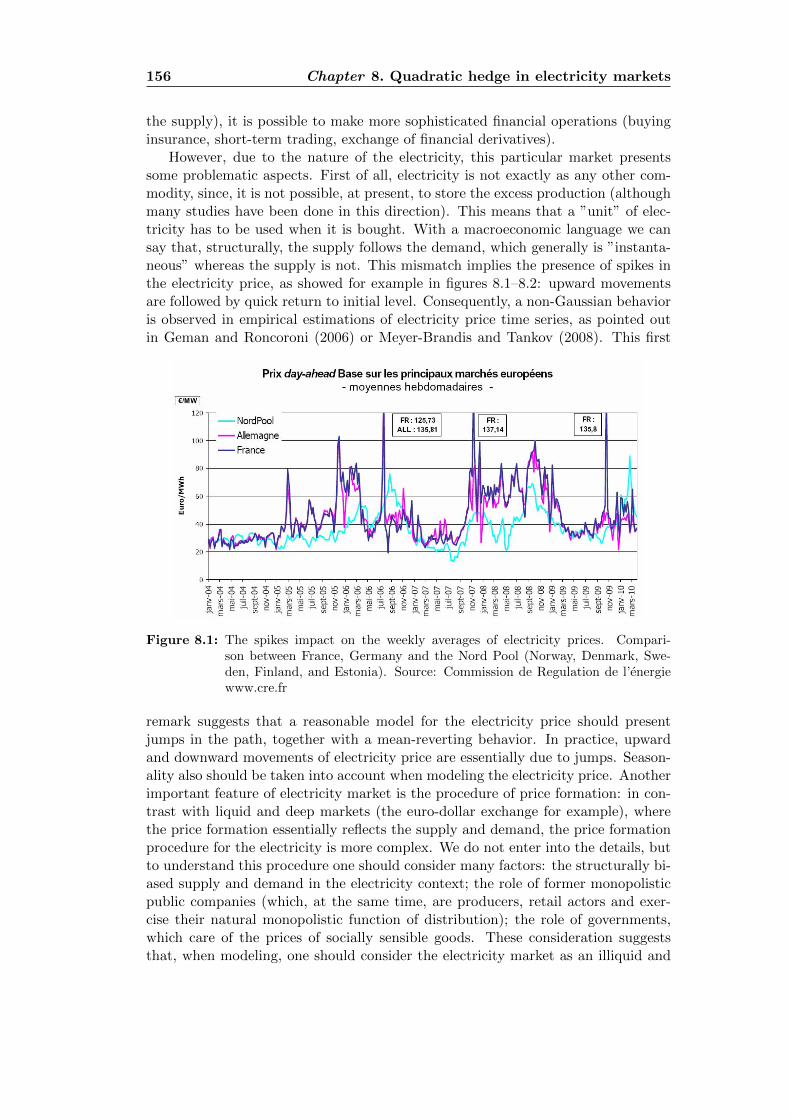
156 Chapter 8. Quadratic hedge in electricity markets
the supply), it is possible to make more sophisticated financial operations (buyinginsurance, short-term trading, exchange of financial derivatives).
However, due to the nature of the electricity, this particular market presentssome problematic aspects. First of all, electricity is not exactly as any other com-modity, since, it is not possible, at present, to store the excess production (althoughmany studies have been done in this direction). This means that a ”unit” of elec-tricity has to be used when it is bought. With a macroeconomic language we cansay that, structurally, the supply follows the demand, which generally is ”instanta-neous” whereas the supply is not. This mismatch implies the presence of spikes inthe electricity price, as showed for example in figures 8.1–8.2: upward movementsare followed by quick return to initial level. Consequently, a non-Gaussian behavioris observed in empirical estimations of electricity price time series, as pointed outin Geman and Roncoroni (2006) or Meyer-Brandis and Tankov (2008). This first
Figure 8.1: The spikes impact on the weekly averages of electricity prices. Compari-son between France, Germany and the Nord Pool (Norway, Denmark, Swe-den, Finland, and Estonia). Source: Commission de Regulation de l’energiewww.cre.fr
remark suggests that a reasonable model for the electricity price should presentjumps in the path, together with a mean-reverting behavior. In practice, upwardand downward movements of electricity price are essentially due to jumps. Season-ality also should be taken into account when modeling the electricity price. Anotherimportant feature of electricity market is the procedure of price formation: in con-trast with liquid and deep markets (the euro-dollar exchange for example), wherethe price formation essentially reflects the supply and demand, the price formationprocedure for the electricity is more complex. We do not enter into the details, butto understand this procedure one should consider many factors: the structurally bi-ased supply and demand in the electricity context; the role of former monopolisticpublic companies (which, at the same time, are producers, retail actors and exer-cise their natural monopolistic function of distribution); the role of governments,which care of the prices of socially sensible goods. These consideration suggeststhat, when modeling, one should consider the electricity market as an illiquid and
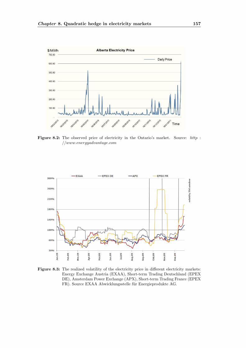
Chapter 8. Quadratic hedge in electricity markets 157
Figure 8.2: The observed price of electricity in the Ontario’s market. Source: http ://www.energyadvantage.com
Figure 8.3: The realized volatility of the electricity price in different electricity markets:Energy Exchange Austria (EXAA), Short-term Trading Deutschland (EPEXDE), Amsterdam Power Exchange (APX), Short-term Trading France (EPEXFR). Source EXAA Abwicklungsstelle fur Energieprodukte AG.
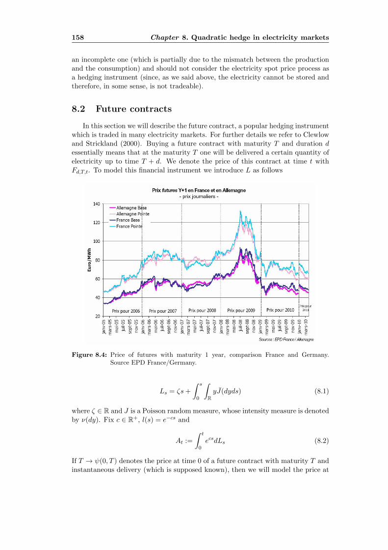
158 Chapter 8. Quadratic hedge in electricity markets
an incomplete one (which is partially due to the mismatch between the productionand the consumption) and should not consider the electricity spot price process asa hedging instrument (since, as we said above, the electricity cannot be stored andtherefore, in some sense, is not tradeable).
8.2 Future contracts
In this section we will describe the future contract, a popular hedging instrumentwhich is traded in many electricity markets. For further details we refer to Clewlowand Strickland (2000). Buying a future contract with maturity T and duration dessentially means that at the maturity T one will be delivered a certain quantity ofelectricity up to time T + d. We denote the price of this contract at time t withFd,T,t. To model this financial instrument we introduce L as follows
Figure 8.4: Price of futures with maturity 1 year, comparison France and Germany.Source EPD France/Germany.
Ls = ζs+
∫ s
0
∫RyJ(dyds) (8.1)
where ζ ∈ R and J is a Poisson random measure, whose intensity measure is denotedby ν(dy). Fix c ∈ R+, l(s) = e−cs and
At :=
∫ t
0ecsdLs (8.2)
If T → ψ(0, T ) denotes the price at time 0 of a future contract with maturity T andinstantaneous delivery (which is supposed known), then we will model the price at
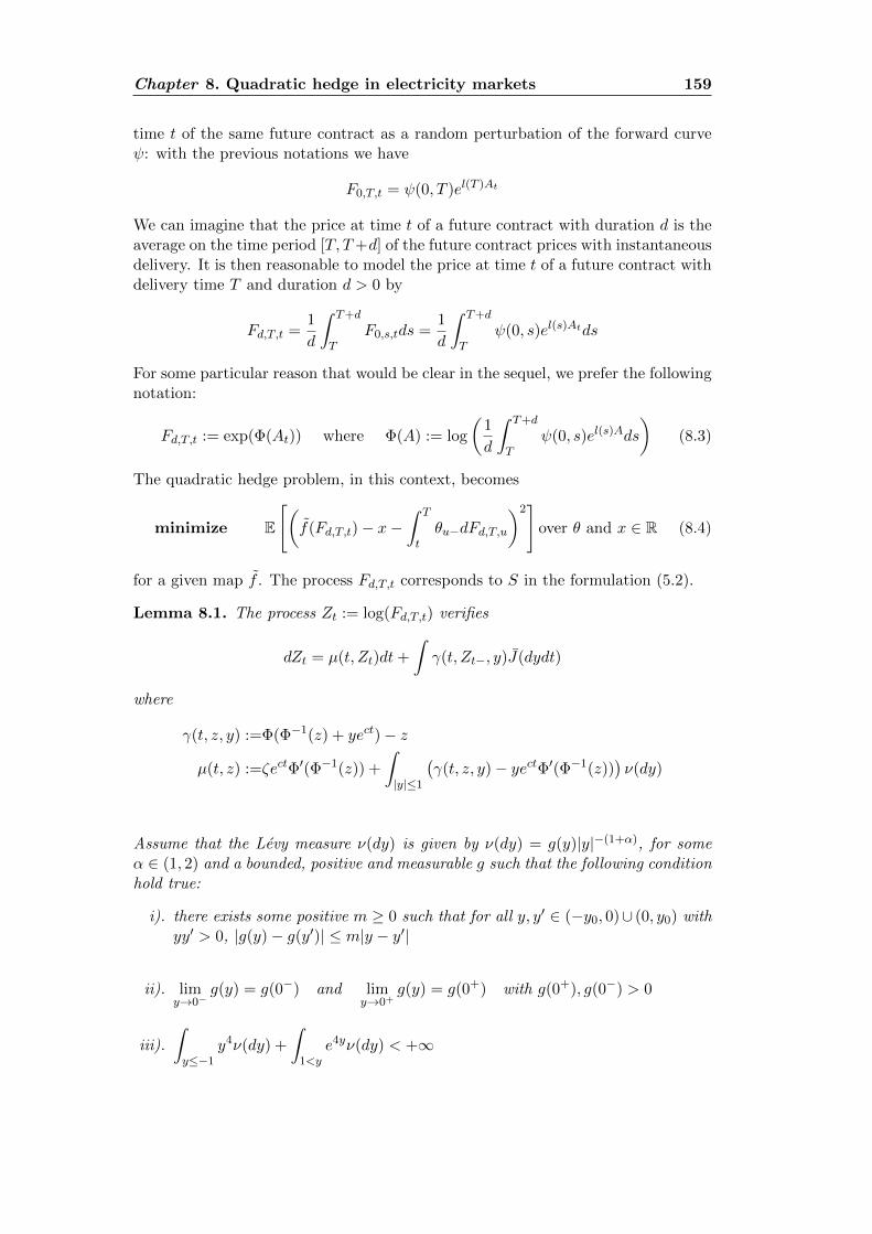
Chapter 8. Quadratic hedge in electricity markets 159
time t of the same future contract as a random perturbation of the forward curveψ: with the previous notations we have
F0,T,t = ψ(0, T )el(T )At
We can imagine that the price at time t of a future contract with duration d is theaverage on the time period [T, T+d] of the future contract prices with instantaneousdelivery. It is then reasonable to model the price at time t of a future contract withdelivery time T and duration d > 0 by
Fd,T,t =1
d
∫ T+d
TF0,s,tds =
1
d
∫ T+d
Tψ(0, s)el(s)Atds
For some particular reason that would be clear in the sequel, we prefer the followingnotation:
Fd,T,t := exp(Φ(At)) where Φ(A) := log
(1
d
∫ T+d
Tψ(0, s)el(s)Ads
)(8.3)
The quadratic hedge problem, in this context, becomes
minimize E
[(f(Fd,T,t)− x−
∫ T
tθu−dFd,T,u
)2]
over θ and x ∈ R (8.4)
for a given map f . The process Fd,T,t corresponds to S in the formulation (5.2).
Lemma 8.1. The process Zt := log(Fd,T,t) verifies
dZt = µ(t, Zt)dt+
∫γ(t, Zt−, y)J(dydt)
where
γ(t, z, y) :=Φ(Φ−1(z) + yect)− z
µ(t, z) :=ζectΦ′(Φ−1(z)) +
∫|y|≤1
(γ(t, z, y)− yectΦ′(Φ−1(z))
)ν(dy)
Assume that the Levy measure ν(dy) is given by ν(dy) = g(y)|y|−(1+α), for someα ∈ (1, 2) and a bounded, positive and measurable g such that the following conditionhold true:
i). there exists some positive m ≥ 0 such that for all y, y′ ∈ (−y0, 0)∪ (0, y0) withyy′ > 0, |g(y)− g(y′)| ≤ m|y − y′|
ii). limy→0−
g(y) = g(0−) and limy→0+
g(y) = g(0+) with g(0+), g(0−) > 0
iii).
∫y≤−1
y4ν(dy) +
∫1<y
e4yν(dy) < +∞

160 Chapter 8. Quadratic hedge in electricity markets
then the functions µ and γ verify the Assumptions 5.1–7.1, where the function τintroduced in Assumption 5.1-[I1] is given by
τ(y) = ecd max (|y|, |ey − 1|)
Furthermore the function γ verifies the Assumptions 7.6-[H1,H3,H4].
Proof.Before we start, remark that the function A 7→ Fd,T (A) is strictly increasing, soinvertible, and infinitely differentiable: in particular
Φ′(A) =
∫ T+dT ψ(0, s)l(s)el(s)Ads∫ T+dT ψ(0, s)el(s)Ads
Φ′′(A) =
(∫ T+dT ψ(0, s)l2(s)el(s)Ads
)(∫ T+dT ψ(0, s)el(s)Ads
)−(∫ T+d
T ψ(0, s)l(s)el(s)Ads)2
(∫ T+dT ψ(0, s)el(s)Ads
)2
from which we deduce
e−c(T+d) ≤ Φ′(A) ≤ e−cT and e−2c(T+d) − e−2cT ≤ Φ′′(A) ≤ e−2cT − e−2c(T+d)
From Ito’s formula, we obtain
dZt =
(Φ′(At)e
ctζ +
∫|y|≤1
(Φ(At− + ecty)− Φ(At−)− yectΦ′(At−)
)ν(dy)
)dt
+
∫R
(Φ(At− + ecty)− Φ(At−)
)J(dydt)
or equivalently
dZt = µ(t, Zt)dt+
∫γ(t, Zt−, y)J(dydt)
We can now prove that µ and γ verify the Assumptions 5.1. We detail the compu-tations only for the function γ, since similar computations can be done for µ. Firstwe remark that z → γ(t, z, y) is differentiable and we can compute this derivativeto obtain
∂zγ(t, z, y) =− 1 + (Φ′(Φ−1(z)))−1Φ′(Φ−1(z) + yect)
=ecty(Φ′(Φ−1(z)))−1
∫ 1
0Φ′′(Φ−1(z) + rect)dr
so that
|∂zγ(t, z, y)| =∣∣∣∣ecty(Φ′(Φ−1(z)))−1
∫ 1
0Φ′′(Φ−1(z) + rect)dr
∣∣∣∣≤|y|ecT (inf
A|Φ(A)|)−1
∥∥Φ′′∥∥∞ ≤ e
cT e−c(T+d)∥∥Φ′′
∥∥∞
≤|y|ecT ec(T+d)(e−2cT − e−2c(T+d)
)≤ ecd|y|
Chapter 8. Quadratic hedge in electricity markets 161
From the bounds on the first and second derivative of Φ we obtain supt,z |∂zγ(t, z, y)| ≤ecd|y|, which gives us the function ρ introduced in Assumptions 5.1. From thebounds on the first and second derivative of Φ we obtain supt,z |∂zγ(t, z, y)| ≤e−cd|y|, which gives us the function ρ introduced in Assumptions 5.1. Also bythe definition of Φ in (8.3) we have
exp(e−c(T+d)y)− 1 ≤ eγ(t,z,y) − 1 ≤ ey − 1
if y > 0 and the inverse inequality stands in force if y < 0, which yield supt,z |eγ(t,z,y)−1| ≤ |ey − 1|. According to the definition of the function τ given in Assumptions5.1 and the estimations above we deduce that
τ (y) := max
(supt,u,z
(|γ (t, z, y) |,
∣∣∣eγ(t,z,y) − 1∣∣∣) , ρ(y)
)= ecd max (|y|, |ey − 1|)
which verifies Assumptions 5.1-[I1, I2] and Assumptions 7.1-[I] from iii). For As-sumption 7.1-[ND] we have, from the definition of γ(
eγ(t,z,y) − 1)2≥(
exp(e−c(T+d)y)− 1)2
so then, for some positive M > 0 we have
Γ(y) :=
∫R
inft,z
(eγ(t,z,y) − 1
)2ν(dy) ≥
∫R
inft,z
(exp(e−c(T+d)y)− 1
)2ν(dy)
≥M∫|y|≤ε|y|1−αg(y)dy > 0
since g(0+) and g(0−) are strictly positive, we can select ε small enough and obtain
Γ(y) ≥M∫|y|≤ε|y|1−αdy > 0
For the Assumptions 7.6 we can differentiate γ w.r.t y to obtain ∂yγ(t, z, y) =
ectΦ′(Φ−1(z) + ecty) so then e−c(T+d) ≤ |∂yγ(t, z, y)| ≤ 1, which proves that As-sumption 7.6-[H1] holds true. For Assumption 7.6-[H3], one can differentiate ∂yγw.r.t. z and give for it an upper bound to prove that z → ∂yγ(t, z, y) is Lipschitzcontinuous, uniformly in t, y. Assumption 7.6-[H4] trivially holds true.
We can transform the problem (8.4) by using the process Z to obtain
vf (t, z, x) = infθ∈X (t,z,x)
E
[(f(Zt,zT )− x−
∫ T
tθu−d exp(Zt,zu )
)2], x, z ∈ R (8.5)
where X (t, z, x) is defined in (5.10) and f(z) = f(ez).In order to apply our results (Theorems 7.14 and 7.17) we need to verify all the
Assumptions 7.6. It is easy to prove that the function γ does not verify Assumption7.6-[H2]: however, as we have already seen, this can be avoided by using Lemma
162 Chapter 8. Quadratic hedge in electricity markets
7.16, whose assumptions are verified by γ. We could change the state variable Zinto a new one, say Z ′, study the problem (8.5) in the new state variable Z ′ (see thediscussion in Section 7.5, page 141) and finally obtain the characterization of theoptimal Markovian strategy as a function of the state variable Z ′. And by applyingthe inverse change of variable, we can express this optimal strategy in terms of Z.From a practical and numerical point of view, one can avoid to make this change ofvariable, and apply directly Theorem 5.14 to obtain the optimal strategy.
To conclude this section, we want to introduce a special class of options one canuse in problem (8.5). First define, for some G > 0 the function p(x) : (G− x)+, theusual put function, and
h(A) :=1
d′
∫ T+d′
Tψ(0, s)el(s)Ads
for some d′ 6= d. From (8.3) it follows that h Φ−1(Zt) = Fd′,T,t, and then, bydefining f := p h Φ−1, we obtain f(Zt) = (G − Fd′,T,t)+, which is a put optionwritten on a future contract with different duration d′. Using this particular optionwe can rewrite problem (8.5) as follows
minimize over θ E
[((G− Fd′,T,t)+ − x−
∫ T
tθu−dFd,T,u
)2]
The financial meaning of the above problem is particularly interesting: one triesto hedge (in the quadratic sense) a put option written on a future contract withduration d′ 6= d only by using, as hedging instrument, the future contract withduration d. This may be useful when, for example, one sells a future contract witha non-standardized duration in the OTC market and hedges its position only byusing the instruments available in the market.
8.3 Numerical approximation of the functions a and b
In this section we will briefly discuss how one can solve the PIDEs obtainedin Theorems 5.11–5.14 in the particular example presented in Section 8.2. Thiswas done with the precious collaboration of Xavier Warin, EDF R&D (De Franco,Tankov, and Warin, 2012).
As we proved in Theorem 7.17, the optimal Markovian strategy in problem (8.5)is given by θ∗t = θ(t, Zt−, Xt−), where
θ∗(t, z, x) :=e−z(π∗(t, z)x− 1
2
Qtb(t, z)Gta(t, z)
)and
π∗(t, z) :=− Qta(t, z)
Gta(t, z)(:= πt[a])
and the optimal price is given in (5.42) x∗ := −b(t, z)(2a(t, z))−1 To solve theproblem then we only need to compute the function a and b, which in this case,
Chapter 8. Quadratic hedge in electricity markets 163
verify
0 =− ∂a
∂t− µ∂a
∂z− Bta− inf
|π|≤Π
2πQta+ π2Gta
, a(T, z) = 1
0 =− ∂b
∂t− µ∂b
∂z− Btb− πt[a]Qtb, b(T, z) = −2f
We will present here a numerical method to approximate the functions a and b.For this, we prefer to rewrite the above PIDEs in a more comfortable way: with anabuse of notation, we first invert the time direction µ(t, z) 7→ µ(T − t, z), and weredefine our operators as follows:
µ(t, z)redef:= µ(t, z) +
∫|y|≥1
γ(t, z, y)ν(dy)
Bϕ(t, z)redef:=
∫R
(ϕ(t, z + γ(t, z, y))− ϕ(t, z, y)− γ(t, z, y)
∂ϕ
∂z(t, z)
)ν(dy)
Qϕ(t, z)redef:=
[µ(t, z) +
∫R
(eγ(t,z,y) − 1− γ(t, z, y)
)ν(dy)
]ϕ(t, z)
+
∫R
(eγ(t,z,y) − 1
)(ϕ(t, z + γ(t, z, y))− ϕ(t, z)) ν(dy)
Gϕ(t, z)redef:=
∫R
(eγ(t,z,y) − 1
)2ϕ(t, z + γ(t, z, y))ν(dy)
In particular, we will write π[ϕ]redef:= −Qϕ(t, z)(Gϕ(t, z))−1, where Q and G are the
redefined operators above. With these notations we obtain the new PIDEs verifiedby a and b
0 =− ∂a
∂t+ µ
∂a
∂z+ Ba+ inf
|π|≤Π
2πQa+ π2Ga
, a(0, z) = 1 (8.6)
0 =− ∂b
∂t+ µ
∂b
∂z+ Bb+ π[a]Qb, b(0, z) = −2f (8.7)
In order to solve the above PIDEs, we need to truncate the domain, i.e. we willnumerically solve the above PIDEs in [0, T ] × [−Z,Z]. Due to the presence of theintegro-differential operator, the boundary conditions must be imposed not only atthe boundary ∂[0, T ]× Z, Z but also outside this parabolic boundary, let us sayon the region [0, T ] × [−Z, −Z] ∪ [Z, Z]. Moreover, we also need to truncate atsome Y the integrals appearing in the definition of the coefficients in (8.6)–(8.7).We finally assume the following condition:
for all t ∈ [0, T ]
Z + supz∈R,y∈[−Y ,Y ]
γ(t, z, y) ≤ Z and − Z + infz∈R,y∈[−Y ,Y ]
γ(t, z, y) ≥ −Z
8.3.1 The algorithm for the function a: truncation and first ap-proximation
The truncation procedure transforms PIDE (8.6) into the following:
164 Chapter 8. Quadratic hedge in electricity markets
• on [0, T ]× [−Z, Z] we solve
∂a
∂t+ supπ∈[−Π,Π]
−µ∂a
∂z− Btra− 2πQtra− π2Gtra
= 0, a(0, z) = 1 (8.8)
where Π is the constant given in (5.44) and the truncated operators are defined asfollows:
Btra(t, z) :=
∫ Y
−Y
(a(t, z + γ(t, z, y))− a(t, z, y)− γ(t, z, y)
∂a
∂z(t, z)
)ν(dy)
µQ(t, z) :=µ(t, z) +
∫ Y
−Y
(eγ(t,z,y) − 1− γ(t, z, y)
)ν(dy)
Qtra(t, z) :=µQ(t, z)a(t, z) +
∫ Y
−Y
(eγ(t,z,y) − 1
)(a(t, z + γ(t, z, y))− a(t, z)) ν(dy)
Gtra(t, z) :=
∫ Y
−Y
(eγ(t,z,y) − 1
)2a(t, z + γ(t, z, y)ν(dy)
• on [0, T ]× [−Z, −Z) ∪ (Z, Z] we impose
a(t, z) := 1
Remark 8.2. The effect of truncating the coefficients in the PIDE has been studiedin Jakobsen and Karlsen (2005) and we refer to it for an error estimation.
The choice of the boundary condition a(t, z) = 1 is motivated as follows: ifexp(Z) was a martingale, this is the value of the function a (see for example Remark5.13). When exp(Z) fails to be a martingale, we should expect that the effect of thedrift term should not be too strong. Alternatively, one can replace the process Z,outside the boundary, by a Levy process, for which the solution can be computedexplicitly (it will be a simple time-dependent function).
We now adapt the methodology proposed by Forsyth et al. (2007) to solve thetruncated PIDE (8.8) on a regular grid zj = j∆z, for some ∆z > 0 and j ∈ (−N,N).We also define two integers j−Z and jZ such that kj ∈ (−Z, Z) if and only ifj−Z < j < jZ . To avoid interpolation of the values of a when estimating theintegral term, we use a space and time dependent grid to define the intervals ofintegration: the integration points yi are chosen to verify γ(t, z, yi(t, z)) = i∆z.(Remark that this is possible since the function γ is invertible in the variable y).For an integer k ≥ 1 we split the region [−Y , Y ] in three domains:
Ω0(t, z) =y|y−k− 1
2(t, z) ≤ y ≤ yk+ 1
2(t, z)
,
Ω1(t, z) =y|yk+ 1
2(t, z) < y < 1 or − 1 < y < y−k− 1
2(t, z)
, (8.9)
Ω2(t, z) = y|1 ≤ |y| ≤ Y ,
The parameter k is used to fit the size of the domain Ω0(t, z). Due to the very highinfinite activity of the jump process near 0, we will numerically fix k equal to 2 or3 whereas Forsyth et al. (2007) take k = 1. We can write then
Btra(t, z) :=
∫Ω0(t,z)
· · ·+∫
Ω1(t,z)· · ·+
∫Ω2(t,z)
. . .
Chapter 8. Quadratic hedge in electricity markets 165
For the first term we define
D(t, z) :=
∫Ω0(t,z)
γ2(t, z, y)ν(dy)
so that ∫Ω0(t,z)
(a(t, z + γ(t, z, y))− a(t, z)− γ(t, z, y)
∂a
∂z(t, z)
)ν(dy)
=D(t, z)
2
∂2a
∂z2+
∫Ω0(t,z)
O(γ3)ν(dy)
Since |γ(t, z, y)| ≤ M |y| around zero for some positive M (see Lemma 8.1), wededuce∫
Ω0(z)
(a(t, z + γ(t, z, y))− a(t, z)− γ(t, z, y)
∂a
∂z(t, z)
)ν(dy)
=D(t, z)
2
∂2a
∂z2+
∫Ω0
O(|y|3)ν(dy) =D(t, z)
2
∂2a
∂z2+O(|yk+1/2(t, z)− y−(k+1/2)|3−α)
=D(t, z)
2
∂2a
∂z2+O(∆z3−α) (8.10)
since for some ξ ∈ Ω0 we have
(2k + 1)∆z =|γ(t, z, yk+1/2(t, z))− γ(t, z, y−(k+1/2)(t, z))|=|∂yγ(t, z, ξ)||yk+1/2(t, z)− y−(k+1/2)|
and ∂yγ is bounded from below.
In the region Ω2, away from zero, we can subdivide the domain in disjointintervals centered in yi and expand the function γ around the integration points yi,as it is done in Forsyth et al. (2007), to obtain∫
Ω2(z)
(a(t, z + γ(t, z, y))− a(t, z)− γ(t, z, y)
∂a
∂z(t, z)
)ν(dy)
=∑yi∈Ω2
ω(t, z, yi)
(a(t, z + γ(t, z, yi))− a(t, z)− γ(t, z, yi)
∂a
∂z
)+O(∆z2)
=∑yi∈Ω2
ω(t, z, yi)
(a(t, z + i∆z)− a(t, z)− z∆z ∂a
∂z
)+O(∆z2)
where
ω(t, z, yi) :=
∫ yi+1/2(t,z)
yi−1/2(t,z)ν(dy), yi ∈ Ω2
For the region Ω1 we need to transform the Levy measure since it has infinite activityclose to zero. Following Forsyth et al. (2007), define ν(dy) := ν(y)y2dy and then

166 Chapter 8. Quadratic hedge in electricity markets
y−2
(a(t, z + γ(t, z, y))− a(t, z)− γ(t, z, y)
∂a
∂z(t, z)
)= y−2
i
(a(t, z + γ(t, z, yi))− a(t, z)− γ(t, z, yi)
∂a
∂z(t, z)
)+ e(i, y)
e(i, y) := (y − yi)d
dy
(y−2
(a(t, z + γ(t, z, y))− a(t, z, y)− γ(t, z, y)
∂a
∂z(t, z)
))|y=yi
+(y − yi)2
2
∫ 1
0dθ∫ θ
0
d2
dy2
(y−2
(a(t, z + γ(t, z, u))− a(t, z, u)− γ(t, z, u)
∂a
∂z(t, z)
)) ∣∣u=yi+r(y−yi) dr
Then, as before,∫Ω1
(a(t, z + γ(t, z, y))− a(t, z)− γ(t, z, y)
∂a
∂z(t, z)
)ν(dy)
=∑
i: yi∈Ω1
ω(t, z, yi)
(a(t, z + γ(t, z, yi))− a(t, z)− γ(t, z, yi)
∂a
∂z(t, z)
)
+∑
i: yi∈Ω1
∫ yi+1/2
yi−1/2
e(i, y)ν(dy)
where
ω(t, z, yi) := y−2i
∫ yi+1/2(t,z)
yi−1/2(t,z)|y|1−αg(y)dy, yi ∈ Ω1
We can use the bound on the function γ and its derivative w.r.t. y to control theerror term (See appendix A in Forsyth et al. (2007))∑
i: yi∈Ω1
∫ yi+1/2
yi−1/2
e(i, y)ν(dy) = O(∆zmin(2−ε,3−α))
for any ε > 0. We finally add up all the above estimations to obtain
Btra(t, z) :=D(t, z)
2
∂2a
∂z2
+∑
yi, |i|>k
ω(t, z, yi)
(a(t, z + i∆z)− a(t, z)− i∆z ∂a
∂z(t, z)
)+O
(∆zmin(2−ε,3−α)
)where
ω(t, z, yi) :=
y−2i
∫ yi+1/2(t,z)
yi−1/2(t,z)|y|1−αg(y)dy if yi+1/2(t, z), yi−1/2(t, z) ∈ Ω1
∫ yi+1/2(t,z)
yi−1/2(t,z)|y|−(1+α)g(y)dy otherwise
(8.11)
Chapter 8. Quadratic hedge in electricity markets 167
The above terms can be calculated with the trapezoidal rule with an integration over5 points, if the function g is twice continuously differentiable with bounded secondderivative away from zero: when yi ∈ Ω1 we obtain an error of order O(∆z3−α)whereas for yi ∈ Ω2 we obtain an error of order O(∆z3).
Similarly we will treat the operators Qtr and Gtr. We skip the details to obtain:
Qtra(t, z) :=µQ(t, z)a(t, z) +D(t, z)∂a
∂z
+∑
yi, |i|>k
IQ(t, z, yi) (a(t, z + i∆z)− a(t, z)) +O(∆zmin(2−ε,3−α))
Gtra(t, z) :=D(t, z)a(t, z) +∑
yi, |i|>k
IG(t, z, yi)a(t, z + i∆z) +O(∆z2−ε)
where
IQ(t, z, yi) :=
y−2i
∫ yi+1/2(t,z)
yi−1/2(t,z)(eγ − 1) |y|1−αg(y)dy if yi+1/2(t, z), yi−1/2(t, z) ∈ Ω1
∫ yi+1/2(t,z)
yi−1/2(t,z)(eγ − 1) |y|−(1+α)g(y)dy otherwise
and
IG(t, z, yi) :=
y−2i
∫ yi+1/2(t,z)
yi−1/2(t,z)(eγ − 1)2 |y|1−αg(y)dy if yi+1/2(t, z), yi−1/2(t, z) ∈ Ω1
∫ yi+1/2(t,z)
yi−1/2(t,z)(eγ − 1)2 |y|−(1+α)g(y)dy otherwise
Again a five point approximation can be used to estimate the above integrals.The above computation allows us to rewrite PIDE (8.8) into the following:
∂a
∂t(t, z)− D(t, z)
2
∂2a
∂z2− µ(t, z)
∂a
∂z+ supπ∈[−Π,Π]
(V (t, z) −2πD(t, z))
∂a
∂z
−∑|i|≥k
W (t, z, yi, π)a(t, z + i∆z) + R(t, z, π)a(t, z)
a(0, z) = 1 (8.12)
where
W (t, z, yi, π) := ω(t, z, yi) + 2πIQ(t, z, yi) + π2IG(t, z, yi)
V (t, z) :=∑|i|≥k
i∆zω(t, z, yi)
R(t, z, π) :=∑|i|>k
(ω(t, z, yi) + 2πIG(t, z, yi)
)− 2πµQ(t, z)− π2D(t, z)
168 Chapter 8. Quadratic hedge in electricity markets
Remark 8.3. The same type of computations can be used to approximate the coef-ficients appearing in the PIDEs (8.6)–(8.7), like, for example,∫
|y|≥1γ(t, z, y)ν(dy) and
∫R
(eγ(t,z,y) − 1− γ(t, z, y)
)ν(dy)
8.3.2 The algorithm for the function a: numerical scheme and con-vergence
Fix n ∈ N, ∆t = T/n and consider tn = n∆t. To solve PIDE (8.12) we use animplicit scheme for linear part, which basically corresponds to a classical diffusion,and an explicit one is used for the integral part: if an stands for a(n∆t, .) then thiswill lead to
an+1 − an
∆t− D(tn+1, .)
2
∂2an+1
∂z2−
µ(tn+1, z)∂an+1
∂z+ supπ∈[−Π,Π]
[(V (tn, .)− 2πD(tn, z))
∂an
∂z+
R(tn, .π)an −∑|i|>k
W (tn, ., yi, π)an(z + i∆z)
= 0 (8.13)
For the implicit term a classical central difference scheme (order two) is used forthe first order differential term coupled with forward/backward differencing whenmatrix coefficients due to diffusion are negative (see for example Forsyth et al.(2005)). The explicit first order differential term is treated to have monotony of thescheme. This transforms equations (8.13) into
an+1j (1 + ∆t(αj(t
n+1) + βj(tn+1))−∆tαj(t
n+1)an+1j−1 −∆tβj(t
n+1)an+1j+1
+ supπ∈[−Π,Π]
[anj (−1 + ∆t(R(tn, zj , π
n) +|V (tn, zj)− 2πD(tn, zj)|
∆z)
−anj−1∆t(V (tn, zj)− 2πD(tn, zj))
+
∆z− anj+1∆t
(V (tn, zj)− 2πD(tn, zj))−
∆z
−∆t∑|i|>k
W (tn, zj , yi, πnj )anj+i
= 0 (8.14)
where an+1j stands for an approximation of an+1(zj) calculated at point zj and αj
and βj are positive weights (see for example Forsyth and Labahn (2007)) given by :
αj,central(t, ) =D(t, zj)
2∆z2− µ(t, zj)
2∆z
βj,central(t) =D(t, zj)
2∆z2+µ(t, zj)
2∆z
if αj,central(t) or βj,central(t, π) is negative, we use
αj,forward/backward(t) =D(t, zj)
2∆z2+max(0,−µ(t, zj)
∆z)
βj,forward/backward(t) =D(t, zj)
2∆z2+max(0,
µ(t, zj)
∆z)
Chapter 8. Quadratic hedge in electricity markets 169
Denote with M the matrix
Mj,j(tn+1) = αj(t
n+1) + βj(tn+1),
Mj,j+1(tn+1) = βj(tn+1),
Mj,j−1(tn+1) = αj(tn+1),
and with B the matrix
Bj,j(tn, π) = R(tn, π, zj) +
|V (tn, zj)− 2πD(tn, zj)|∆z
,
Bj,j−1(tn, π) = −(V (tn, zj)− 2πD(tn, zj))+,
Bj,j+1(tn, π) = −(V (tn, zj)− 2πD(tn, zj))−,
Bj,j+i(tn, π) = −W (tn, π, zj , yi), if |i| > k,
Bj,j+i(tn, π) = 0, for 1 < |i| ≤ k,
The system can be written in terms of these matrices:
(I + ∆tM(tn+1))an+1 + supπ∈(−Π,Π)
(−I + ∆tB(tn, π))an = 0 (8.15)
Theorem 8.4. Under the CFL condition
supt,j
[V (t, zj)
∆z+ 2Π(|µ(t, zj)|+D(t, zj))+
∑|i|>k
(2ΠIQ(t, zj , yi) + ω(t, zj , yi)) + Π2D(t, zj))+
∆t < 1
the scheme 8.15 is consistent, monotone, L∞ stable and converges to the viscositysolution of equation (8.8).
The proof of this result can be found in De Franco, Tankov, and Warin (2012). Wejust remark that the integer k ≥ 1 in (8.9) is chosen to improve the convergenceof the scheme. This is needed since the jump activity of the process may be veryhigh, and then the error we do in our approximations (in the Taylor expansionsas, for example, in (8.10), or in the approximated integrals as (8.11)) can be veryimportant. Taking k ≥ 1 means that we extend the critical region Ω0(t, z) in (8.9)and this allows us to be more precise.
8.3.3 Resolution methodology to calculate the function b
We will use the same methodology developed in paragraphs 8.3.1–8.3.2 for thePIDE (8.7): we first rescale the function b to b(t, z) := e−ηtb(t, z) and then weproceed by truncating the domain of definition of b to obtain the new PIDE:
• on [−Z, Z] ∂b
∂t− µ∂b
∂z− Btr b+ ηb− πtr[a]Qtrb = 0
b(0, z) = −2f(z)(8.16)
where πtr[a] := −Qtra(Gtra
)−1
170 Chapter 8. Quadratic hedge in electricity markets
• on [−Z, −Z) ∪ (Z, Z] we impose
b(t, z) = −2f(z)a(t, z)e−ηt
Remark 8.5. The choice of the boundary condition outside the domain is justifiedas follows: the value −b(t, z)/2a(t, z) can be interpreted as the cost of hedging thepay-off f , that is, the wealth at time t which leads to the minimal hedging error atmaturity, as stated in (5.42). In the regions far from the money (and under theassumption of zero interest rate), the cost of hedging can be approximated by theoption’s pay-off, whence the boundary condition for b.
Using the same discretization as before we get the following equation to solveon [−Z,Z]:
∂b
∂t− D(t, z)
2
∂2b
∂z2+∂b
∂z
((V (t, z)− µ(t, z)− πtr[a]D(t, z)
)+b(η + R(t, z, πtr[a])
)−∑|i|≥k
W (t, z, yi, πtr[a])b(t, z + i∆z)
b(0, z) = −2f(z) (8.17)
where
W (t, z, yi, πtr[a]) := ω(t, z, yi) + πtr[a]IQ(t, z, yi)
R(t, z, πtr[a]) :=∑|i|>k
(ω(t, z, yi) + πtr[a]IQ(t, z, yi)
)− πtr[a]µQ(t, z)
and V and D(t, z) are the functions introduced in paragraph 8.3.1. We propose, asin paragraph 8.3.2, the following time discretization scheme :
bn+1 − bn
∆t− D(tn+1, .)
2
∂2bn+1
∂z2+
(V (tn+1, .)− π[a]n+1D(tn+1, z)− µ(tn+1, z))∂bn+1
∂z+ (R(tn+1, ., π[a]n+1) + η)bn+1 −∑
|i|>k
(W (tn+1, ., yi, π[a]n+1))+bn(z + i∆z) +
∑|i|>k
(W (tn+1, ., yi, π[a]n+1))−bn(z + i∆z) = 0
which becomes
bn+1j (1 + ∆t(αj(t
n+1) + βj(tn+1) + R(tn+1, zj , π[a]n+1) + η)−
∆tαj(tn+1)bn+1
j−1 −∆tβj(tn+1)bn+1
j+1 + ∆t∑|i|>k
(W (tn+1, zj , yi, π[a]n+1))−bn+1j+i
−∆t∑|i|>k
(W (tn+1, zj , yi, π[a]n+1))+bnj+i = 0 (8.18)

Chapter 8. Quadratic hedge in electricity markets 171
where bnj is the approximated value of b at (tn, zj), and αj , βj positive weights givenby :
αj,central(t, π) =D(t, zj)
2∆z2+V (t, .)− πD(t, z)− µ(t, zj)
2∆z
βj,central(t, π) =D(t, zj)
2∆z2− V (t, .)− πD(t, z)− µ(t, zj)
2∆z
if αj,central(t, π) or βj,central(t, π) is negative, we use
αj,forward/backward(t, π) =D(t, zj)
2∆z2+
(V (t, .)− πD(t, z)− µ(t, zj)
∆z
)+
βj,forward/backward(t, π) =D(t, zj)
2∆z2+
(V (t, .)− πD(t, z)− µ(t, zj)
∆z
)−Proposition 8.6. For a space discretization accurate enough (∆z small enough),taking
η = (Π + ε) ‖µ‖∞ + 2
∫|y|>1
(1 + Π|ey − 1|)ν(dy)
the scheme (8.18) is consistent and stable so it converges to the viscosity solutionof the PIDE (8.16).
Again, the proof of the above result is given in De Franco, Tankov, and Warin(2012). Remark that this result is not the same of Theorem 8.4: the function bdepends on a through the optimal control π, for which we do not control the sign.This has an important impact on the convergence of the Scheme for b.
8.4 A numerical example
In this last paragraph we will study the problem (8.5) when L in (8.1) is aNormal Inverse Gaussian process with parameter α, β, δ, µ: Lt ∼ NIG(α, β, δt, µt).
Remark 8.7. Remark that α should not be mistaken for the parameter in Lemma8.1; similarly µ is not the drift function given in the same Lemma. We use thisnotation because it is standard in the literature.
We can write then
Lt =
(µ+
βδ
α2 − β2+
∫|y|≥1
yν(dy)
)t+
∫ t
0
∫RyJ(dyds)
where J is a Poisson random measure with intensity
ν(dy) =αδ
π|y|K1(α|y|)eβydy ν(dy)
y→0∼ 1
|y|2dy
ν(dy)y→+∞∼ 1
|y|3/2e−(α−β)ydy ν(dy)
y→−∞∼ 1
|y|3/2e−(α+β)|y|dy
where K1 is the modified Bessel function of the second kind (paragraph 4.4.3 inCont and Tankov (2004)).
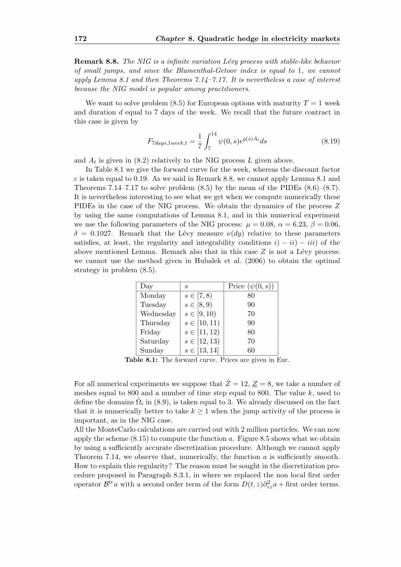
172 Chapter 8. Quadratic hedge in electricity markets
Remark 8.8. The NIG is a infinite variation Levy process with stable-like behaviorof small jumps, and since the Blumenthal-Getoor index is equal to 1, we cannotapply Lemma 8.1 and then Theorems 7.14–7.17. It is nevertheless a case of interestbecause the NIG model is popular among practitioners.
We want to solve problem (8.5) for European options with maturity T = 1 weekand duration d equal to 7 days of the week. We recall that the future contract inthis case is given by
F7days,1week,t =1
7
∫ 14
7ψ(0, s)eg(s)Atds (8.19)
and At is given in (8.2) relatively to the NIG process L given above.In Table 8.1 we give the forward curve for the week, whereas the discount factor
c is taken equal to 0.19. As we said in Remark 8.8, we cannot apply Lemma 8.1 andTheorems 7.14–7.17 to solve problem (8.5) by the mean of the PIDEs (8.6)–(8.7).It is nevertheless interesting to see what we get when we compute numerically thesePIDEs in the case of the NIG process. We obtain the dynamics of the process Zby using the same computations of Lemma 8.1, and in this numerical experimentwe use the following parameters of the NIG process: µ = 0.08, α = 6.23, β = 0.06,δ = 0.1027. Remark that the Levy measure ν(dy) relative to these parameterssatisfies, at least, the regularity and integrability conditions i) − ii) − iii) of theabove mentioned Lemma. Remark also that in this case Z is not a Levy process:we cannot use the method given in Hubalek et al. (2006) to obtain the optimalstrategy in problem (8.5).
Day s Price (ψ(0, s))
Monday s ∈ [7, 8) 80Tuesday s ∈ [8, 9) 90Wednesday s ∈ [9, 10) 70Thursday s ∈ [10, 11) 90Friday s ∈ [11, 12) 80Saturday s ∈ [12, 13) 70Sunday s ∈ [13, 14] 60
Table 8.1: The forward curve. Prices are given in Eur.
For all numerical experiments we suppose that Z = 12, Z = 8, we take a number ofmeshes equal to 800 and a number of time step equal to 800. The value k, used todefine the domains Ωi in (8.9), is taken equal to 3. We already discussed on the factthat it is numerically better to take k ≥ 1 when the jump activity of the process isimportant, as in the NIG case.All the MonteCarlo calculations are carried out with 2 million particles. We can nowapply the scheme (8.15) to compute the function a. Figure 8.5 shows what we obtainby using a sufficiently accurate discretization procedure. Although we cannot applyTheorem 7.14, we observe that, numerically, the function a is sufficiently smooth.How to explain this regularity? The reason must be sought in the discretization pro-cedure proposed in Paragraph 8.3.1, in where we replaced the non local first orderoperator Btra with a second order term of the form D(t, z)∂2
zza+ first order terms.
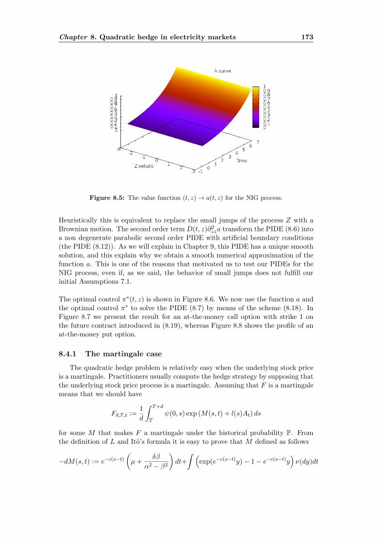
Chapter 8. Quadratic hedge in electricity markets 173
Figure 8.5: The value function (t, z)→ a(t, z) for the NIG process.
Heuristically this is equivalent to replace the small jumps of the process Z with aBrownian motion. The second order term D(t, z)∂2
zza transform the PIDE (8.6) intoa non degenerate parabolic second order PIDE with artificial boundary conditions(the PIDE (8.12)). As we will explain in Chapter 9, this PIDE has a unique smoothsolution, and this explain why we obtain a smooth numerical approximation of thefunction a. This is one of the reasons that motivated us to test our PIDEs for theNIG process, even if, as we said, the behavior of small jumps does not fulfill ourinitial Assumptions 7.1.
The optimal control π∗(t, z) is shown in Figure 8.6. We now use the function a andthe optimal control π∗ to solve the PIDE (8.7) by means of the scheme (8.18). InFigure 8.7 we present the result for an at-the-money call option with strike 1 onthe future contract introduced in (8.19), whereas Figure 8.8 shows the profile of anat-the-money put option.
8.4.1 The martingale case
The quadratic hedge problem is relatively easy when the underlying stock priceis a martingale. Practitioners usually compute the hedge strategy by supposing thatthe underlying stock price process is a martingale. Assuming that F is a martingalemeans that we should have
Fd,T,t :=1
d
∫ T+d
Tψ(0, s) exp (M(s, t) + l(s)At) ds
for some M that makes F a martingale under the historical probability P. Fromthe definition of L and Ito’s formula it is easy to prove that M defined as follows
−dM(s, t) := e−c(s−t)(µ+
δβ
α2 − β2
)dt+
∫ (exp(e−c(s−t)y)− 1− e−c(s−t)y
)ν(dy)dt
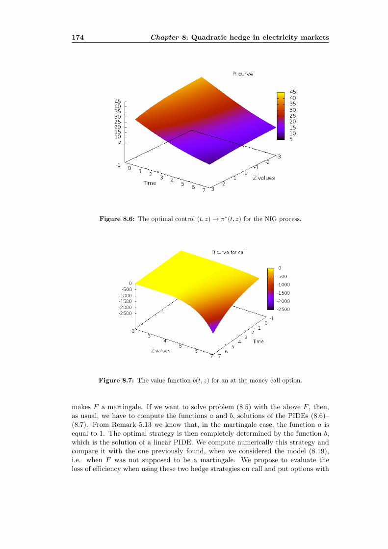
174 Chapter 8. Quadratic hedge in electricity markets
Figure 8.6: The optimal control (t, z)→ π∗(t, z) for the NIG process.
Figure 8.7: The value function b(t, z) for an at-the-money call option.
makes F a martingale. If we want to solve problem (8.5) with the above F , then,as usual, we have to compute the functions a and b, solutions of the PIDEs (8.6)–(8.7). From Remark 5.13 we know that, in the martingale case, the function a isequal to 1. The optimal strategy is then completely determined by the function b,which is the solution of a linear PIDE. We compute numerically this strategy andcompare it with the one previously found, when we considered the model (8.19),i.e. when F was not supposed to be a martingale. We propose to evaluate theloss of efficiency when using these two hedge strategies on call and put options with
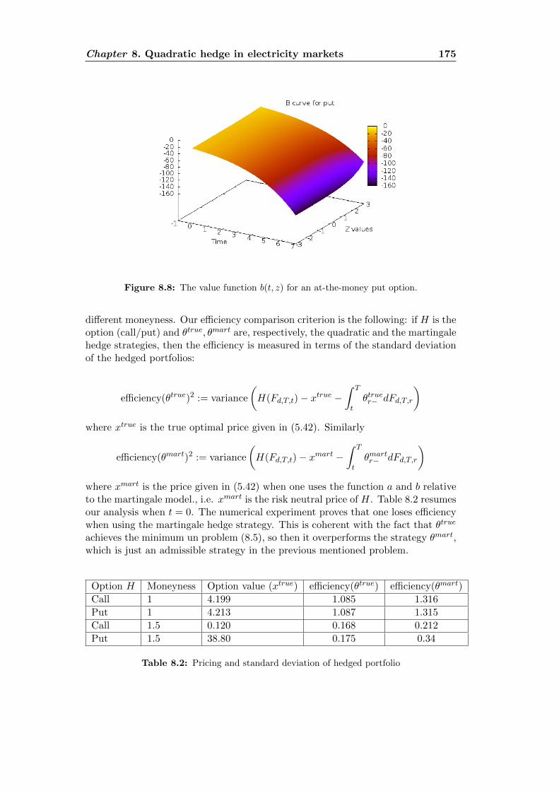
Chapter 8. Quadratic hedge in electricity markets 175
Figure 8.8: The value function b(t, z) for an at-the-money put option.
different moneyness. Our efficiency comparison criterion is the following: if H is theoption (call/put) and θtrue, θmart are, respectively, the quadratic and the martingalehedge strategies, then the efficiency is measured in terms of the standard deviationof the hedged portfolios:
efficiency(θtrue)2 := variance
(H(Fd,T,t)− xtrue −
∫ T
tθtruer− dFd,T,r
)where xtrue is the true optimal price given in (5.42). Similarly
efficiency(θmart)2 := variance
(H(Fd,T,t)− xmart −
∫ T
tθmartr− dFd,T,r
)where xmart is the price given in (5.42) when one uses the function a and b relativeto the martingale model., i.e. xmart is the risk neutral price of H. Table 8.2 resumesour analysis when t = 0. The numerical experiment proves that one loses efficiencywhen using the martingale hedge strategy. This is coherent with the fact that θtrue
achieves the minimum un problem (8.5), so then it overperforms the strategy θmart,which is just an admissible strategy in the previous mentioned problem.
Option H Moneyness Option value (xtrue) efficiency(θtrue) efficiency(θmart)
Call 1 4.199 1.085 1.316
Put 1 4.213 1.087 1.315
Call 1.5 0.120 0.168 0.212
Put 1.5 38.80 0.175 0.34
Table 8.2: Pricing and standard deviation of hedged portfolio

Chapter 9
The PIDE truncation effect
The chapter is organized as follows: we start by explaining why it is important tostudy the semi linear PIDE verified by the value function of the pure investmentproblem, when one truncates the domain of solvability (Section 9.1). For this, wefirst provide an approximation of this value function by cutting the small jumpsof the Levy measure and replace them with a term involving the second derivative,and then we prove the convergence of this approximation to the true value function(Section 9.2). We then prove that the truncated PIDE relative to this approximationhas a unique smooth solution (Section 9.3), and we finally prove an estimate on theerror due to the truncation of the domain (Section 9.4).
Contents
9.1 Motivations . . . . . . . . . . . . . . . . . . . . . . . . . . . 1779.2 A first approximation . . . . . . . . . . . . . . . . . . . . . 1799.3 The semi linear PIDE on a bounded domain . . . . . . . 182
9.3.1 Existence and Uniqueness in the viscosity sense . . . . . . 1829.3.2 Existence and Uniqueness in the viscosity sense . . . . . . 184
9.4 Estimate on the truncated PIDE . . . . . . . . . . . . . . 191
9.1 Motivations
In the example proposed in Chapter 8 we showed how to solve the PIDEs (8.6)–(8.7) to obtain the value function and the optimal control of problem (8.5). Ourtheoretical results ensured that these PIDEs have a smooth classical solution onthe domain [0, T ]×R. Nevertheless, in order to implement a numerical scheme, weneeded to truncate the solvability domain of these PIDEs: we consider (8.6)–(8.7) ina bounded domain of the form [0, T ]× [−Z,Z] with artificial Dirichlet conditions atthe boundary. It is then natural to ask whenever these truncated PIDEs still havea smooth solution and how the artificial boundary conditions affect the solution.
To simplify the presentation we consider the model of Chapter 6 and we assumethat the process Z in (5.5) does not depend on U . We will also concentrate onthe PIDE verified by the function a, since a similar approach can be used for b.Remark that, from a practical point of view, one only needs of a and b to compute
177
178 Chapter 9. The PIDE truncation effect
the optimal strategy of problem (5.11), which is given in (5.50).
We recall that if a denotes the function in (5.13), then (t, z) → a(t, z)eηt is theunique solution of
0 = −∂a∂t
+ ηa+Ata− Bta−H[a], a(T, z) = eηT
and it belongs to C(1−δ)/2+1,2+(1−δ)([0, T ] × R), for any η ≥ 0. From a numericalpoint of view one is instead interested in
0 = −∂a∂t
+ ηa+Ata− Bta−Ht[a] (t, z) ∈ [0, T )× (−Z, Z)
a(T, z) = eηT z ∈ (−Z, Z)
a(t, z) = eηtq(t, z) (t, z) ∈ [0, T ]× (−Z, Z)c
(9.1)
for some artificial Dirichlet boundary condition q. Remark that it is possible toconsider a more general domain of the form (Z1, Z2): in general the choice of thedomain depends on the particular needs of the numerical discretization. However,it is important for the sequel that the domain has a smooth boundary: in theone dimensional case this is trivially true if one considers open intervals. For themultidimensional case one should consider, for example, bounded cylinders. Theabove truncated PIDE naturally arises when one wants to compute numericallythe function a. Our aim is then to prove that it has a unique solution, whichalso is smooth inside the domain, and give some estimate of the error between thefunction a and the solution of the above PIDE. The analysis of this PIDE may bevery difficult when the intensity measure is not finite. This is related to the behaviorof the non local operator
(t, z)→ Ba(t, z) :=
∫ (a(t, z + γ(t, z, y))− a(t, z)− γ(t, z, y)
∂a
∂z(t, z)1|y|≤1
)ν(dy)
when z reaches the boundary of the truncated domain. Heuristically, we can remarkthat the operator B behaves as ∂2
zza(t, z)+ ”first order operator”. Since there is nohope to prove that the solution of PIDE (9.1) is twice continuously differentiableat the boundary [0, T ] × −Z,Z, the operator B will be not properly defined onthe above boundary, and the map (t, z) → Ba(t, z), for |z| ≤ Z, may fail to beuniformly Holder continuous. Much more tractable is the case when the intensitymeasure ν(dy) is finite. For this, before considering the truncated PIDE (9.1), weshow how to transform the initial parameters of the model (5.5), (µ, σ2, γ, ν(dy)) inorder to obtain a finite intensity measure. As we will see in Section 9.2, this is doneby cutting the small jumps of the process Z and ”replace” them with a Brownianmotion, as we did in Paragraph 8.3.1. This replacing transforms, at the same time,the jump measure of the process into a finite intensity measure and the volatilityfunction σ. Our task then reduces to considering the value function of the pureinvestment problem when the process Z has finite jumps. In the sequel, we willdenote this new function ah, where h > 0 is the level at which we cut the smalljumps. A first result is to prove that this new value function ah converges to the
Chapter 9. The PIDE truncation effect 179
function a when h → 0. In Section 9.3 we then study the truncated PIDE whichcharacterizes the function ah, which has the same structure as PIDE (9.1), exceptfor the fact that the non local operators are all of order zero.
Throughout the chapter we denote ΩT := [0, T ] × [−Z,Z] and fT := [0, T ] ×(−Z,Z)c. Moreover, for a function ϕ defined on ΩT , ‖ϕ‖l/2,l,ΩT denotes the Holder
norm of ϕ relatively to ΩT : for example,
‖ϕ‖∞,ΩT := supt≤T,|z|≤Z
|ϕ(t, z)| and 〈ϕ〉(l)z,ΩT
:= sup(t,z),(t,z′)∈ΩT
|ϕ(t, z)− ϕ(t, z′)||z − z′|l
The same convention stands in force for the Holder norm of type 2, and for theHolder norm on the domain fT .
9.2 A first approximation
Let h > 0 and consider
γh(t, z) :=
∫|y|≤h
γ2(t, z, y)ν(dy)
Assumptions 5.1–6.1 on γ show that γh is bounded, Lipschitz continuous w.r.t. tand z and that γh → 0 when h→ 0, uniformly in t, z. Since
Bϕ(t, z) =
∫ 1
0dθ
∫ θ
0dθ′∫|y|≤h
γ2∂2ϕ
∂z2(t, z + θ′γ(t, z, y))ν(dy)
+
∫|y|>h
(ϕ(t, z + γ(t, z, y))− ϕ(t, z)− γ(t, z, y)
∂ϕ
∂z(t, z)1|y|≤1
)ν(dy)
then we could replace the above operator with
γh(t, z)
2
∂2ϕ
∂z2(t, z) +
∫|y|>h
(ϕ(t, z + γ(t, z, y))− ϕ(t, z)− γ(t, z, y)
∂ϕ
∂z(t, z)1|y|≤1
)ν(dy)
This is equivalent to consider the pure investment problem (5.13) with the newparameters (
µ, σ2 + γh, γ, ν(dy)1|h|<y
)(9.2)
If ah denotes the value function of the pure investment problem corresponding tothese initial parameters, then from Theorems 5.11–6.8 we obtain that the map(t, z)→ ah(t, z)eηt is the unique solution of
0 = −∂ah
∂t+ ηah +Aht ah − Bht ah −Hh[ah], ah(T, z) = eηT (9.3)
180 Chapter 9. The PIDE truncation effect
provided that T < T ∗,h, where T ∗,h is the maximal time given in Theorem 5.4relatively to the new parameters. The above operators are given by
Aht ah :=− µ∂ah
∂z− 1
2
(σ2 + γh
) ∂2ah
∂z2
Bht ah :=
∫h<|y|
(ah(t, z + γ)− ah(t, z)− γ ∂a
h
∂z1|y|≤1
)ν(dy)
Qht ah :=µhah +(σ2 + γh
) ∂ah∂z
+
∫h<|y|
(eγ − 1)(ah(t, z + γ)− ah(t, z)1|y|≤1
)ν(dy)
Ght ah :=(σ2 + γh
)ah +
∫h<|y|
(eγ − 1)2ah(t, z + γ)ν(dy)
Hht [ah] := inf|π|≤Πh
2πQht ah + π2Ght ah
(9.4)
where µh is given in (5.6) with the new parameters and Πh in (5.38) is the a prioribound corresponding to the new parameters. The main advantage when consideringthe value function ah is due to the fact that the intensity measure is now finite andthen we could write, for example,
Bht ah =
∫h<|y|
(ah(t, z + γ)− ah(t, z)
)ν(dy)− ∂ah
∂z
∫h<|y|≤1
γ(t, z, y)ν(dy)
It is relatively easy to check the regularity of the right hand side when z approachesthe boundary of the truncated domain. Our aim now is to prove that the function ah
converges in some functional space to a and the optimal control (πh)∗ also convergesto π∗, the optimal control relative to the function a. For this we will suppose that
T < T ∗ ∧ T ∗,h (9.5)
in order to guarantee that both a and ah are smooth solutions of their respectivePIDEs.
Theorem 9.1. Let Assumptions 5.1–6.1 hold true together with the condition (9.5).Then
i).∥∥a− ah∥∥
2−δ,H ≤Mη%(h)
ii).∥∥π∗ − (πh)∗
∥∥1−δ,H ≤Mη%(h)
where (πh)∗ is the optimal control given in (5.47) relatively to ah, M(η) is a positiveconstant that depends on η > 0 but not on h and %(h) is the function introduced inLemma 6.2:
%(h) :=
∫|y|≤h
τ2(y)ν(dy)→ 0, when h→ 0
Proof.From Proposition 6.5 we know that there exists a sequence ϕn ∈ C1+(1−δ)/2,2+(1−δ)([0, T ]×R) that converges in H2−δ([0, T ]× R) to a:
‖ϕn − a‖2−δ,H → 0, n→∞
Chapter 9. The PIDE truncation effect 181
and the same holds true when considering the function ah:∥∥∥ϕn,h − ah∥∥∥2−δ,H
→ 0, n→∞
where ϕn,h is another sequence that also belongs to C1+(1−δ)/2,2+(1−δ)([0, T ] × R).Since∥∥∥a− ah∥∥∥
2−δ,H≤ ‖ϕn − a‖2−δ,H +
∥∥∥ϕn − ϕn,h∥∥∥2−δ,H
+∥∥∥ϕn,h − ah∥∥∥
2−δ,H(9.6)
we can concentrate on the middle term∥∥ϕn − ϕn,h∥∥
2−δ,H . Let M denote a positiveconstant that does not depend on η or h whereas Mη is a positive constant thatdoes depend on η but not on h. They may change from line to line.
If ∆nh := ϕn − ϕn,h then we can write
− ∂
∂t4n+1h +Aht4n+1
h + η4n+1h = Bht4n
h +Ht[ϕn]−Hht [ϕn,h]
−1
2γh∂2ϕn+1
∂2z+
∫|y|≤h
(ϕn(t, z + γ)− ϕn(t, z)− γ ∂ϕ
n
∂z1|y|≤1
)ν(dy)
4n+1h (T, z) = 0
where we basically used the definition of these sequences stated in (6.3).First we can estimate the second derivative appearing in the above PDE:∥∥∥∥∥1
2γh∂2ϕn+1
∂2z−∫|y|≤h
(ϕn(t, z + γ)− ϕn(t, z)− γ ∂ϕ
n
∂z1|y|≤1
)ν(dy)
∥∥∥∥∥∞
≤M supn‖ ϕn‖2,H
∫|y|≤h
τ2(y)ν(dy) ≤Mη%(h) (9.7)
by using Lemma 6.9. We can proceed as in the proof of Lemma 6.2 to prove thatfor any r, ε > 0∥∥∥Bh4n
h
∥∥∥∞≤M
((%(r) + ς(r)ε1−δ
)‖4n
h‖2−δ,H + ς(r)ε−1 ‖4nh‖∞
)(9.8)
where ς(r) → ∞ if the function τ is not integrable around zero. To conclude, wereadapt the proof of Lemma 6.3 and obtain∥∥∥H[ϕn]−Hh[ϕn,h]
∥∥∥∞≤M
(∥∥∥Qϕn −Qhϕn,h∥∥∥∞
+∥∥∥Gϕn − Ghϕn,h∥∥∥
∞
)≤M
(‖4n
h‖1+λ,H + %(h) ‖ϕn‖2,H)
for some 0 < λ < 1 − δ, where we used the structure of the operators Q,G andQh,Gh. Apply then Proposition C.3 to deduce∥∥∥H[ϕn]−Hh[ϕn,h]
∥∥∥∞≤M
(ε1−δ−λ ‖4n
h‖2−δ,H + ε−(1+λ) ‖4nh‖∞ + %(h) ‖ϕn‖2,H
)We now use the above estimation and (9.7)–(9.8) as in the proof of Proposition 6.5to obtain, for some η big enough and some β ∈ (0, 1)∥∥4n+1
h
∥∥2−δ,H,η ≤ β ‖4
nh‖2−δ,H,η +M(η)%(h)
182 Chapter 9. The PIDE truncation effect
where, as usual, ‖ ‖2−δ,H,η := ‖ ‖2−δ,H + η ‖ ‖∞. It follows then∥∥4n+1h
∥∥2−δ,H,η ≤M(η)
(βn+1 + %(h)
)Finally, we use the above estimate in (9.6) and let n → ∞ to prove part i). Forpart ii) we have ∥∥∥π∗ − (πh)∗
∥∥∥1−δ,H
=
∥∥∥∥QaGa − QhahGhah
∥∥∥∥1−δ,H
Using the estimation given in i) and the structure of the above operators it is notdifficult to prove that ∥∥∥π∗ − (πh)∗
∥∥∥1−δ,H
≤M(η)%(h)
Remark that the optimal control depends on the first derivative of a: this explainswhy we can just give an estimate on the Holder norm of order 1− δ.
This result proves that we can approximate with arbitrary precision the valuefunction a and the optimal control π∗ by taking h small enough. This allows us tostudy the truncated PIDE for ah instead of a.
9.3 The semi linear PIDE on a bounded domain
9.3.1 Existence and Uniqueness in the viscosity sense
From now on we assume fixed h > 0. We start by making some simplificationsin the definition of the differential operators in (9.4): define first µh(t, z) := µ(t, z)−∫h<|h|≤1 γ(t, z, y)ν(dy), then redefine the operators as follows:
Aht ahredef:= − µh∂a
h
∂z− 1
2
(σ2 + γh
) ∂2ah
∂z2
Bht ahredef:=
∫h<|y|
(ah(t, z + γ)− ah(t, z)
)ν(dy)
Qht ahredef:=
(µh +
1
2
(σ2 + γh
))ah +
(σ2 + γh
) ∂ah∂z
+
∫h<|y|
(eγ − 1) ah(t, z + γ)ν(dy)
Ght ahredef:=
(σ2 + γh
)ah +
∫h<|y|
(eγ − 1)2ah(t, z + γ)ν(dy)
Hht [ah]redef:= inf
|π|≤Πh
2πQht ah + π2Ght ah
(9.9)
The function (t, z)→ ah(t, z)eηt verifies
0 = −∂ah
∂t+ ηah +Aht ah − Bht ah −Hh[ah], ah(T, z) = eηT (9.10)
From the above definition we remark that the non local operators are all of orderzero, which will substantially simplify our computations. Remark however that at
Chapter 9. The PIDE truncation effect 183
this point we cannot let anymore h→ 0, since the above coefficients and operatorsmay not be properly defined if the Levy measure ν is infinite. According to Theorem9.1, we assume then that h > 0 is selected and fixed in order to have a suitablysmall error when replacing the function a with ah.
Remark 9.2. From now on, all the constants appearing in our estimates maydepend on h.
As we already anticipated in Section 9.1, let Z > 0 and consider the problem (9.10)in the bounded parabolic domain [0, T ]× [−Z, Z]:
0 = −∂atr
∂t+ ηatr +Aht atr − Bht atr −Hh[atr] (t, z) ∈ [0, T )× (−Z, Z)
atr(T, z) = eηT z ∈ (−Z, Z)
atr(t, z) = eηtq(t, z) (t, z) ∈ [0, T ]× (−Z, Z)c
(9.11)
Here the superscript tr stands for truncated. In the rest of the Chapter we willprove that the above PIDE has a unique solution which is smooth in the domain[0, T ] × [−Z, Z] and give an estimate on the error between atr and ah. One canthen use Theorem 9.1 to deduce an estimate on the error between atr and a.
Note that, due to the non local component, the Dirichlet condition q has to bespecified on the entire domain [0, T ] × (−Z, Z)c. We assume that q has the sameregularity as the function ah outside the domain1: q ∈ C(1−δ)/2+1,2+(1−δ)(fT ) and
limt→T,|z|≥Z
q(t, z) = 1 (9.12)
to ensure continuity at time t = T .
Lemma 9.3. Under Assumptions 5.1–6.1 there exists a unique viscosity solutionof PIDE (9.11). If (9.12) also holds true then it is continuous and it assumes theboundary condition in the classical sense.
Proof.The result is a direct application2 of Theorem 3 in Barles, Chasseigne, and Imbert(2008). Remark that we would have a unique viscosity solution even under lessconstraining Assumptions.
1This is actually not necessary and one could consider some other Dirichlet boundary conditionthat belongs to C(1−δ′)/2+1,2+(1−δ′)(fT ) for some δ′ ∈ (0, 1). We prefer to take q in the same spaceof ah for sake of coherence.
2Theorem 3 in Barles, Chasseigne, and Imbert (2008) proves existence and uniqueness for ellipticdifferential problems. However, as the authors precise in Section 4.3 of the same paper, the proofcan be easily adapted to the parabolic case.
184 Chapter 9. The PIDE truncation effect
9.3.2 Existence and Uniqueness in the viscosity sense
In this paragraph we will first prove that the unique viscosity solution of PIDE(9.11) belongs to C2−δ(ΩT ). This will allow us to remove the non linearity inthe PIDE (9.11) and finally prove that this unique viscosity solution belongs toC1+(1−δ)/2,2+(1−δ)(ΩT ).
For this, we will need to assume that the function q verifies a compatibilitycondition at time t = T . Condition (9.12) gives the continuity of q, but we also haveto impose that the derivative w.r.t. t of the function atr, which can be computedfrom the equation and the initial conditions, is equal to the derivative of the Dirichletboundary condition. In particular one must have
∂atr
∂t(T, z) = ηeηT −Hh[atr(T, z)]
from (9.11). If we impose that
∂eηtq
∂t(T, z) =
∂atr
∂t(T, z), z ∈ −Z,Z
then we should have
∂q
∂t(T, z) =
(Qhatr(T, z)
)2Ghatr(T, z)
, z ∈ −Z,Z
By using the terminal condition of atr and the definition of Ah and Gh, we willobtain
∂q
∂t(T, z)
=
((µ+ 1
2σ2)
+∫R((eγ − 1− γ1|y|≤1
)1|h|<y + 1
2γ21|y|≤h
)ν(dy)
)2σ2 +
∫h<|y|
((eγ − 1)21|h|<y + γ21|y|≤h
)ν(dy)
(9.13)
where the coefficients are evaluated at the point (T, z) and z ∈ −Z,Z. We alsoneed to assume some regularity on the function γ and σ:
There exists δ′ ∈ (0, 1) such that ∂zσ, ∂zγ ∈ Hδ′([0, T ]× R), for any t, y. (9.14)
We will explain later where these assumptions are needed. Define then
κ := min(1− δ, δ′) (9.15)
As we already did many times (see Sections 6.2.2–7.4.1), we prove that the uniqueviscosity solution of PIDE (9.11) belongs to C1+(1−δ)/2,2+(1−δ)(ΩT ) by introducinga sequence of smooth function ϕn and proving that it converges to the uniqueviscosity solution in the above mentioned Holder space. Let us start with someϕ0 ∈ Hκ/2+1,2+κ([0, T ]× R) and consider (ϕn)n∈N defined by
ϕn+1(t, z) :=
ϕn+1(t, z) (t, z) ∈ [0, T ]× [−Z, Z]
eηtq(t, z) (t, z) ∈ [0, T ]× [−Z, Z]c(9.16)
where ϕn+1 verifies
Chapter 9. The PIDE truncation effect 185
−∂ϕn+1
∂t+ ηϕn+1 +Ahϕn+1 = Bht ϕn −Hh[ϕn] (t, z) ∈ [0, T )× (−Z, Z)
ϕn+1(T, z) = eηT z ∈ (−Z, Z)
ϕn+1(t, z) = eηtq(t, z) (t, z) ∈ [0, T ]× −Z, Z
(9.17)
Remark 9.4. From now on we will adopt the following notation: for any functionψ : ΩT → R, we denote with ψ the extension of this map on the domain [0, T ]× Rwith the Dirichlet boundary condition:
ψn+1(t, z) :=
ψn+1(t, z) (t, z) ∈ [0, T ]× [−Z, Z]
eηtq(t, z) (t, z) ∈ [0, T ]× [−Z, Z]c
Our first objective is to prove that the sequence in (9.16) is well defined. For thiswe need a preliminary result on the properties on the operators Bh and Hh:
Lemma 9.5. Let Assumptions 5.1–6.1 hold true. There exists some positive con-stant M > 0 such that for all ψ ∈ Cκ/2+1,2+κ(ΩT ) we have∥∥∥Bhϕn∥∥∥
∞,ΩT≤M
(‖ϕn‖∞,ΩT + eηT ‖q‖∞,fT
)∥∥∥Hh[ϕn]
∥∥∥∞,ΩT
≤M(‖ϕn‖1,H,ΩT + eηT ‖q‖∞,fT
)and ∥∥∥Bhϕn∥∥∥
κ/2,κ,ΩT≤M
(‖ϕn‖κ/2,κ,ΩT + eηT ‖q‖κ/2,κ,fT
)∥∥∥Hh[ϕn]
∥∥∥κ/2,κ,ΩT
+∥∥∥Qhϕn∥∥∥
κ/2,κ,ΩT+∥∥∥Ghϕn∥∥∥
κ/2,κ,ΩT≤
M(‖ϕn‖(κ+1)/2,1+κ,ΩT + eηT ‖q‖κ/2,κ,fT
)where ψ denotes the extension of ψ according to the Remark 9.4. The constant Mdoes not depend on η.
Proof.The proof can be completed with the type of computations we made for Lemmas6.2–6.3, by using the fact that outside the domain ΩT , the map ψ is equal to eηtq.
The only difference arises when one has to estimate 〈Bhϕn〉(κ)
z,ΩT(or 〈Hhϕn〉(κ)
z,ΩTand
so on), since one has to take into account the particular form of ψ. We detail this
computation for 〈Bhϕn〉(κ)
z,ΩT: we first have
〈Bhϕn〉(κ)
z,ΩT≤∫h<|y|〈ϕn(t, z + γ(t, z, y))− ϕn(t, z)〉(κ)
z,ΩTν(dy)
186 Chapter 9. The PIDE truncation effect
Fix z, z′ ∈ [−Z,Z]: it follows∣∣ϕn(t, z + γ(t, z, y))− ϕn(t, z)− ϕn(t, z′ + γ(t, z′, y)) + ϕn(t, z′)∣∣
≤〈ϕn〉(κ)
z,ΩT|z − z′|κ +
∣∣ϕn(t, z + γ(t, z, y))− ϕn(t, z′ + γ(t, z′, y))∣∣
If z + γ(t, z, y), z′ + γ(t, z′, y) ∈ (−Z,Z) then∣∣ϕn(t, z + γ(t, z, y))− ϕn(t, z′ + γ(t, z′, y))∣∣ ≤M(1 + ρ(y)κ)|z − z′|κ〈ϕn〉(κ)
z,ΩT
If instead z + γ(t, z, y) ∈ (−Z,Z) but z′ + γ(t, z′, y) /∈ (−Z,Z), then we can findsome λ ∈ [0, 1] such that zλ +γ(t, zλ, y) ∈ [0, T ]×Z,Z, where zλ := z+λ(z′− z).This is due to the continuity of the map z → γ(t, z, y). We deduce then∣∣ϕn(t, z + γ(t, z, y))− ϕn(t, z′ + γ(t, z′, y))
∣∣≤ |ϕn(t, z + γ(t, z, y))− ϕn(t, zλ + γ(t, zλ, y))|+∣∣ϕn(t, zλ + γ(t, zλ, y))− ϕn(t, z′ + γ(t, z′, y))
∣∣≤M(1 + ρ(y)κ)|z − zλ|κ
(〈ϕn〉(κ)
z,ΩT+ 〈q〉(κ)
fT
)≤M(1 + ρ(y)κ)|z − z′|κ
(〈ϕn〉(κ)
z,ΩT+ eηT 〈q〉(κ)
fT
)Finally, if both are outside the interval (−Z,Z) then, we can distinguish two cases
• both z+ γ(t, z, y) and z′+ γ(t, z′, y) are on the same side w.r.t. (−Z,Z), andthen∣∣ϕn(t, z + γ(t, z, y))− ϕn(t, z′ + γ(t, z′, y))
∣∣ ≤M(1 + ρ(y)κ)eηT |z − z′|κ〈q〉(κ)
fT
• one is bigger than Z whereas the other is smaller that −Z: in this case thetriangular inequality yields∣∣ϕn(t, z + γ(t, z, y))− ϕn(t, z′ + γ(t, z′, y))
∣∣≤M(1 + ρ(y)κ)|z − z′|κ
(〈ϕn〉(κ)
z,ΩT+ eηT 〈q〉(κ)
fT
)Adding up all the above estimates we obtain
〈Bhϕn〉(κ)
z,ΩT≤M
(‖ϕn‖κ/2,κ,ΩT + eηT ‖q‖κ/2,κ,fT
)The same argument can be used to estimate 〈Bhϕn〉((κ)/2)
t,ΩT.
The above Lemma allows us to prove that the sequence in (9.16) is well defined.Assume that the compatibility conditions (9.12)–(9.13) hold true. By recurrence, ifϕn ∈ Cκ/2+1,2+κ(ΩT ) is well defined then Lemma 9.5 yields
Bhϕn +Hh[ϕn] ∈ Cκ/2,κ(ΩT )
Chapter 9. The PIDE truncation effect 187
We can use Theorem 5.2, Chapter IV in Ladyzenskaja et al. (1967) to deduce thatPIDE (9.17) has a unique solution which belongs to Cκ/2+1,2+κ(ΩT ). This provesthat ϕn+1 is also well defined. Furthermore
∥∥ϕn+1∥∥κ2
+1,2+κ,ΩT≤M
(eηT +
∥∥∥Bhϕn +Hh[ϕn]∥∥∥κ/2,κ,ΩT
+∥∥eηtq∥∥κ
2,2+κ,fT
)Remark 9.6. The function ϕn is Lipschitz continuous at the boundary [0, T ] ×−Z,Z: since ϕn ∈ Cκ/2+1,2+κ(ΩT ) then
∥∥Dzϕn+1∥∥∞,ΩT is finite. But
∥∥Dz(eηtq)
∥∥∞,fT
is also finite for any t ≤ T . This means that the function z → ϕn+1(t, z) is contin-uous and has bounded left and right derivatives on the boundary [0, T ] × −Z,Z,which proves that ϕn+1 is Lipschitz continuous on [0, T ]× −Z,Z.
The analog of Proposition 6.5 is this case it the following:
Proposition 9.7. Let Assumptions 5.1–6.1 hold true together with the compatibilityconditions (9.12)–(9.13). Assume also that condition (9.14) stands in force. For ηbig enough, the sequence ϕn defined in (9.16) converges to some ϕ∗ ∈ H2−δ(ΩT ).Furthermore for any υ ∈ (0, 1) there exists some positive constant Mυ which dependson υ such that ∣∣ϕ∗(t, z)− ϕ∗(t′, z)∣∣ ≤Mυ|t− t′|υ, for any t, t′, z
and ∣∣Dzϕ∗(t, z)−Dzϕ
∗(t′, z)∣∣ ≤Mυ|t− t′|υ/2, for any t, t′, z
Proof.If 4n+1 := ϕn+1 − ϕn and 4n+1 := ϕn+1 − ϕn then
−∂4n+1
∂t+ η4n+1 +Ah4n+1 = Bht 4n +Hh[ϕn]−Hh[ϕn−1] (t, z) ∈ [0, T )× (−Z, Z)
ϕn+1(T, z) = 0 z ∈ (−Z, Z)
ϕn+1(t, z) = 0 (t, z) ∈ [0, T ]× −Z, Z
The unique solution of the above linear PDE is explicitly given in Ladyzenskajaet al. (1967), Section §16,
4n+1(t, z) =
∫ T
te−η(s−t)ds
∫ Z
−ZG(T − t, z, T − s, ξ)Rn(y, ξ)dξ (9.18)
where Rn := Bh4n + Hh[ϕn] − Hh[ϕn−1] and G the Green’s function given inTheorem 16.3 of Ladyzenskaja et al. (1967), Chapter IV, §16, which verifies
i). For 2r + s ≤ 2,
∣∣DitD
jyG(t, z, s, ξ)
∣∣ ≤ m1(t− s)−1+2i+j
2 exp
(−m2
|z − ξ|2
t− s
)
188 Chapter 9. The PIDE truncation effect
ii). For 2i+ j = 2 and any ι ∈ (0, 1)
∣∣DitD
jzG(t, z, s, ξ)−Di
tDjzG(t, z′, s, ξ)
∣∣ ≤ m1|z − z′|ι(t− s)−3+ι2 exp
(−m2
|z′′ − ξ|2
t− s
)
Here z′′ is the closest point to ξ which belongs to the segment−→zz′.
iii). For 2i+ j = 1, 2 and s < t′ < t.∣∣DitD
jzG(t, z, s, ξ)−Di
tDjzG(t′, z, s, ξ)
∣∣ ≤m1|t′ − s|−3+ι2 |t− t′|
2−2i−j+ι2
exp
(−m2
|w − ξ|2
s− t
)
for 0 ≤ s < t and positive constants m1,m2.
We can follow the scheme of the proof of Proposition 6.5 to deduce that (ϕn)nis a Cauchy sequence in H2−δ(ΩT ). There exists then some ϕ∗ ∈ H2−δ(ΩT ) suchthat ϕn → ϕ∗.
Let us now prove the regularity of ϕ∗ w.r.t. t. From (9.18) we can write, for t′ < t,∣∣4n+1(t, z)−4n+1(t′, z)∣∣
≤‖Rn‖∞,ΩT∫ T
te−η(s−t)
∫ Z
−Z
∣∣G(T − t, z, T − s, ξ)−G(T − t′, z, T − s, ξ)∣∣ dξds
+ ‖Rn‖∞,ΩT∫ t
t′e−η(s−t′)
∫ Z
−Z
∣∣G(T − t′, z, T − s, ξ)∣∣ dξds
+ ‖Rn‖∞,ΩT∣∣∣eη(t′−t) − 1
∣∣∣ ∫ T
te−η(s−t)
∫ Z
−Z
∣∣G(T − t′, z, T − s, ξ)∣∣ dξds
By using Lemma 6.4 we have∫ Z
−Z
∣∣G(T − t, z, T − s, ξ)−G(T − t′, z, T − s, ξ)∣∣ dξ ≤M
but also∫ Z
−Z
∣∣G(T − t, z, T − s, ξ)−G(T − t′, z, T − s, ξ)∣∣ dξ ≤M |t− t′||s− t|−1
so that∫ Z
−Z
∣∣G(T − t, z, T − s, ξ)−G(T − t′, z, T − s, ξ)∣∣ dξ ≤Mυ|t− t′|υ|s− t|−υ
The first term in the right hand side is then estimated with∫ T
te−η(s−t)
∫ Z
−Z
∣∣G(T − t, z, T − s, ξ)−G(T − t′, z, T − s, ξ)∣∣ dξds ≤Mυ|t− t′|υ
Chapter 9. The PIDE truncation effect 189
For the second it is straightforward∫ t
t′e−η(s−t′)
∫ Z
−Z
∣∣G(T − t′, z, T − s, ξ)∣∣ dξds ≤M |t− t′|
whereas for the third one, there is some λ ∈ [0, 1] such that∣∣∣eη(t′−t) − 1∣∣∣ ∫ T
te−η(s−t)
∫ Z
−Z
∣∣G(T − t′, z, T − s, ξ)∣∣ dξds
≤M |t− t′|ηeλη(t′−t)∫ T
te−η(s−t)ds ≤M |t− t′|
since t′ < t. We conclude then∣∣4n+1(t, z)−4n+1(t′, z)∣∣ ≤Mυ ‖Rn‖∞,ΩT |t− t
′|υ
for some positive Mυ which depends on υ. We can finally readapt the argument ofthe proof of Proposition 6.5 to prove that the sequence of functions t → ϕn(t, .) isalso a Cauchy sequence in the Holder space Hυ ([0, T ]), and then its limit, ϕ∗, hasto belong to this space. In particular∣∣ϕ∗(t, z)− ϕ∗(t′, z)∣∣ ≤Mυ|t− t′|υ, for any t, t′, z
With the same type of computations we prove that the sequence of functions t →Dzϕ
n(t, z) is a Cauchy sequence in the Holder space Hυ/2 ([0, T ]) for any υ ∈ (0, 1).It follows that also Dzϕ
∗ has to belongs to this space.
Corollary 9.8. Let Assumptions 5.1–6.1 hold true together with the compatibilityconditions (9.12)–(9.13). Let ϕ∗ be the limit in H2−δ(ΩT ) of the sequence ϕn. Itsextension to [0, T ]× R, ϕ∗ is the unique viscosity solution of PIDE (9.11):
ϕ∗(t, z) = atr(t, z) (9.19)
Proof. We define
ψ(t, z) := E
[∫ βt,z
te−η(s−t)
(Bht ϕn −Hh[ϕn]
)(s, Zt,zs ) + eηβ
t,zq(βt,z, Zt,z
βt,z
)]
where βt,z is the hitting time of the boundary:
βt,z := T ∧ infs > t :
∣∣∣Zt,zs ∣∣∣ ≥ Z (9.20)
anddZt,zs := µh(s, Zt,zs )ds+
(√σ2 + γh
)(s, Zt,zs )dWs, Zt,zt = z
Remark that from the Markov property of the process Z we have
βt,z = βθ,Zt,zθ for any stopping time t ≤ θ ≤ βt,z
190 Chapter 9. The PIDE truncation effect
In particular, according to Remark 9.4, we can write
ψ(t, z) := E[∫ θ
te−η(s−t)
(Bht ϕn −Hh[ϕn]
)(s, Zt,zs )ds+ eηθψ
(θ, Zt,zθ
)]As in Step 3 of the proof of Theorem 6.8, we deduce that ψ is the unique viscositysolution3 of (9.17). Since ϕn+1 is the unique smooth solution of (9.17), we deduceψ = ϕn+1, and then
ϕn+1(t, z) := E[∫ θ
te−η(s−t)
(Bht ϕn −Hh[ϕn]
)(s, Zt,zs )ds+ eηθϕn+1
(θ, Zt,zθ
)]Since ϕn → ϕ∗ in H2−δ(ΩT ) (Proposition 9.7) and the operators Bh and Hh arebounded and continuous, we can let n→∞ and obtain
ϕ∗(t, z) := E[∫ θ
te−η(s−t)
(Bht ϕ∗ −Hh[ϕ∗]
)(s, Zt,zs ) + eηθϕ∗
(θ, Zt,zθ
)]For t = T we have ϕ∗(T, z) = ϕ∗(T, z) = eηT , by construction of the sequence ϕn,which converges to ϕ∗. If instead |z| ≥ Z, i.e., we are outside the domain, thentrivially βt,z = t, from which we deduce ϕ(t, z) = eηtq(t, z). Again by following theStep 3 of the proof of Theorem 6.8 we deduce that ϕ∗ is a viscosity solution of PIDE(9.11): form the uniqueness of this solution (Lemma 9.3) we deduce
ϕ∗(t, z) = atr(t, z)
We are now able to prove the main result of this chapter:
Theorem 9.9. Let Assumptions 5.1–6.1 stand in force and assume also that thefunctions σ and γ verify (9.14). If the Dirichlet boundary condition q belongs toC(1−δ)/2+1,2+(1−δ)(fT ) and verifies the compatibility conditions (9.12)–(9.13), thenthe PIDE (9.11) has a unique solution atr which verifies
atr∣∣∣ΩT ∈ Cκ/2+1,κ+2(ΩT )
where κ is given in (9.15). Trivially
atr∣∣∣fT ∈ Cκ/2+1,κ+2(fT )
since q belongs to this space, and z → atr(t, z) is Lipschitz continuous for all t ≤ T .
Proof.The only thing we need to prove is that atr
∣∣ΩT ∈ Cκ/2+1,κ+2(ΩT ) . Remark that
Hh[atr] = 2πtrQhatr + (πtr)2Gatr
3According to the definition of viscosity solution, one replaces the function ψ with a twicecontinuously differentiable test function, for which we can apply Ito’s formula. Then we do notneed to take care of the non smoothness of ψ at the boundary (0, T ) × −Z,Z. In other words,the Feynman-Kac formula holds true and gives a probabilistic representation of the function ϕn+1.
Chapter 9. The PIDE truncation effect 191
where
πtr := −Πh ∨ −Qhatr
Gatr∧ Πh (9.21)
from the definition of Hh[atr] in (9.9). Proposition 9.7, Corollary 9.8 and the regu-larity of q imply that πtr ∈ C(1−δ)/2,1−δ([0, T ] × R) and in particular, from (9.15),we have πtr ∈ Cκ/2,κ([0, T ] × R). This allows us to linearize the PIDE (9.11): asalready seen many times, we define the map Ξη(ψ) as follows
−∂Ξη(ψ)
∂t+ ηΞη(ψ) +AhΞη(ψ) = Bht ψ + 2πtrQhψ + (πtr)2Ghψ [0, T )× (−Z, Z)
Ξη(ψ)(T, z) = eηT z ∈ (−Z, Z)
Ξη(ψ)(t, z) = eηtq(t, z) [0, T ]× −Z, Z
for ψ ∈ Cκ/2+1,2+κ(ΩT ). Theorem 5.2, Chapter IV in Ladyzenskaja et al. (1967)guarantees that this map is well defined in Cκ/2+1,2+κ(ΩT ). We can now proceedas in Step 2 of the proof of Theorem 6.8 to deduce that, for η big enough, the mapΞη is a contraction in n Cκ/2+1,2+κ(ΩT )4. If call ψ∗ its unique fixed then, accordingto Remark 9.4, it verifies
−∂ψ∗
∂t+ ηψ∗ +Ahψ∗ = Bht ψ∗ + 2πtrQhψ∗ + (πtr)2Ghψ∗ (t, z) ∈ [0, T )× (−Z, Z)
ψ∗(T, z) = eηT z ∈ (−Z, Z)
ψ∗(t, z) = eηtq(t, z) (t, z) ∈ [0, T ]× −Z, Z
Since atr is the unique viscosity solution of the above PIDE (Lemma 9.3) we deducethat ψ∗ = atr, i.e. the restriction to ΩT of atr belongs to Cκ/2+1,2+κ(ΩT ). Thisproves that PIDE (9.11) has a unique solution, whose restriction to ΩT belongsto Cκ/2+1,2+κ(ΩT ). It is clear that this solution atr is Lipschitz continuous atthe boundary: we already know that it was continuous (Lemma 9.3), and sincethe derivative w.r.t. z of atr and q are bounded, we deduce that atr is Lipschitzcontinuous at the boundary. Clearly atr = q outside the boundary.
9.4 Estimate on the truncated PIDE
Theorem 9.9 tells us that there exists a unique solution of PIDE (9.11), whichis smooth in ΩT . For the remainder of this section we will concentrate on the errorestimation between the function ah introduced in Section 9.2 and the function atr.
4This is done by writing the Feynman-Kac formula for Ξη(ψ), and we explained in the proof ofCorollary 9.8 how it can be done.
192 Chapter 9. The PIDE truncation effect
For this, we will prove that the function atr is the value function of a stochasticoptimization problem. Let us start with the definition of ah:
x2ah(t, z) := infθ∈X (t,z,x)
E[(Xt,z,x,θT
)2]
where X is the wealth process given in (5.9) corresponding to the new parametersin (9.2), and X (t, z, x) is the set of admissible strategies in (5.10). The function ah
belongs to Cκ/2+1,2+κ([0, T ]×R) and the optimal control π∗,h of the above stochasticproblem is given in (5.47). In particular
x2ah(t, z) := infθ∈ET (t,z,x)
E[(Xt,z,x,θT
)2]
where
Eα(t, z, x) :=
θs := θ(s, Zt,zs−, X
t,z,x,θs−
) ∣∣∣∣∣∣θ(t, z, x) := e−zπ(t, z)x and
π ∈ C(1+κ)/2,1+κ([0, T ]× R), t ≤ s ≤ α
since the optimal control π∗,h belongs to the above subset of admissible strategies.Furthermore for any stopping times t ≤ α ≤ T we have
x2ah(t, z) := infθ∈Eα(t,z,x)
E[(Xt,z,x,θα
)2ah(α,Zt,zα
)](9.22)
Remark that this is the dynamic programming principle when we restrict ourselvesto the Markovian strategies in E(t, z, x). The following result proves that atr canalso be represented as in (9.22).
Lemma 9.10. Let the Assumptions of Theorem 9.9 hold true. Then
x2atr(t, z) = infθ∈Eβ(t,z,x)
E[(Xt,z,x,θβt,z
)2q(βt,z, Zt,zβt,z
)]where
βt,z := T ∧ infs > t;
∣∣Zt,zs ∣∣ ≥ Z (9.23)
and Z is the process given in (5.5) when using the parameters in(9.2).
Proof.Let us define the Markovian strategy
θtrs := πtr(s, Zt,zs−)e−Zt,zs−Xt,z,x,θtr
s− , Xt,z,x,θtr
s := x+
∫ s
tθtrs−de
−Zt,zs− (9.24)
where πtr is the optimal control given in (9.21) and
w(t, z, x) := E
(x+
∫ βt,z
tθtrr−de
−Zt,zs−
)2
q(βt,z, Zt,zβt,z
) := x2ϕ(t, z)
Chapter 9. The PIDE truncation effect 193
The flow (t, z) → Zt,z· is continuous in the topology of uniform convergence oncompacts (Theorem 37, Chapter V, Protter (2004)), so then (t, z)→ βt,z is at leastlower semi-continuous (Theorem 38, Chapter V, Protter (2004)). It follows that(t, z, x)→ w(t, z, x) is continuous w.r.t. x and at least measurable w.r.t (t, z). Letnow α ∈
[t, βt,z
]be a stopping time: it follows
w(t, z, x) =E
EFα(x+
∫ α
tθtrr−de
−Zt,zs− +
∫ βt,z
αθtrr−de
−Zt,zs−
)2
q(βt,z, Zt,zβt,z
)=E
EFαXt,z,x,θtr
α +
∫ βα,Zt,zα
αθtrr−de
−Zt,zs−
2
q
(βα,Z
t,zα , Zt,z
βα,Zt,zα
)=E
[w(α,Zt,zα , Xt,z,x,θ
α
)]since the strategy θtr is Markovian. As in the proof of Theorem 6.8 we deduce thatϕ is a viscosity solution of PIDE (9.11) for η = 0, and then, from the uniqueness,ϕ = atr. It follows then
x2atr(t, z) =E
(1 +
∫ βt,z
tθtrr−de
−Zt,zs−
)2
q(βt,z, Zt,zβt,z
)≥ infθ∈Eβ(t,z,x)
E[(Xt,z,x,θβt,z
)2q(βt,z, Zt,zβt,z
)]If now
x2atr(t, z) > infθ∈Eβ(t,z,x)
E[(Xt,z,x,θβt,z
)2q(βt,z, Zt,zβt,z
)]then there would exist some π ∈ C(1+κ)/2,1+κ([0, T ]× R) such that
x2atr(t, z) > E[(Xt,z,xβt,z
)2q(βt,z, Zt,zβt,z
)]:= x2ψ(t, z)
where dXt,z,xs := Xt,z,x
s− π(s, Zt,zs−)e−Zt,zs−deZ
t,zs , Xt,z,x
t = x. It is not complicated to
prove that ψ is the unique solution of
−∂ψ∂t
+Ahψ = Bht ψ + 2πQhψ + π2Ghψ (t, z) ∈ [0, T )× (−Z, Z)
ψ(T, z) = 1 z ∈ (−Z, Z)
ψ(t, z) = q(t, z) (t, z) ∈ [0, T ]× (−Z, Z)c
and it belongs to C1+κ/2,2+κ(ΩT ). See for example the computations we did in theproof of Theorem 9.9. Since atr verifies the PIDE (9.11) we deduce that ϕ := ψ−atrshould verify
194 Chapter 9. The PIDE truncation effect
−∂ϕ∂t
+Ahϕ− Bht ϕ− 2πQhϕ− π2Ghϕ = F (t, z) ∈ [0, T )× (−Z, Z)
ϕ(T, z) = 0 z ∈ (−Z, Z)
ϕ(t, z) = 0 (t, z) ∈ [0, T ]× (−Z, Z)c
where F (t, z) :=(2πQhatr + π2Ghatr −Hh[atr]
)(t, z) ≥ 0 for all (t, z), simply from
the definition of Hh[atr] in (9.9). We can also rearrange the terms in the left handside of the above PIDE in the following way:
µnew(t, z) :=−(µh + 2π
(σ2 + γh
))σnew(t, z) :=
√σ2 + γh
rnew(t, z) :=− 2π
(µh +
1
2
(σ2 + γh
)+
∫h<|y|
(eγ − 1) ν(dy)
)
− π2
(σ2 + γh +
∫h<|y|
(eγ − 1)2 ν(dy)
)νnew(t, z, dy) := (1 + π (eγ − 1))2 ν(dy)1h<|y|
where µh stands for µh(t, z) and so on. With these notations we can write
−∂ϕ∂t− µnew
∂ϕ
∂z− 1
2σ2new
∂2ϕ
∂z2− Bnewϕ− rnewϕ = F (t, z) ∈ [0, T )× (−Z, Z)
ϕ(T, z) = 0 z ∈ (−Z, Z)
ϕ(t, z) = 0 (t, z) ∈ [0, T ]× (−Z, Z)
where Bnew is the non local operator when one uses the Levy measure νnew. TheFeynman-Kac formula5 yields
ϕ(t, z) = E
[∫ βt,z
tF (s, Znew,t,zs ) exp
(∫ s
trnew(u, Znew,t,zu )du
)ds
](9.25)
where
dZnew,t,zs =µnew(s, Znew,t,zs )ds+ σnew(s, Znew,t,zs )dWs
+
∫γ(s, Znew,t,zs− , y)J (s, Znew,t,zs− , dyds)
and J is a Poisson random measure such that, for all Borel set O whose closuredoes not contain zero and any t, z, the process
ξs := J (t, z, [0, s]×O)−∫ s
t
∫O∩|y|>h
(1 + π(t, z)
(eγ(t,z,y) − 1
))2ν(dy)
5See the proof of Corollary 9.8 to justify the Feynman-Kac formula for PIDE in truncateddomains.
Chapter 9. The PIDE truncation effect 195
is a martingale. From (9.25) and F ≥ 0 we deduce ϕ := ψ − atr ≥ 0, which is acontradiction since we assumed that atr(t, z) > ψ(t, z). It follows then that
x2atr(t, z) ≤ infθ∈Eβ(t,z,x)
E[(Xt,z,x,θβt,z
)2q(βt,z, Zt,zβt,z
)]which concludes the proof.
We conclude the chapter with an estimate on the error ah − atr:
Theorem 9.11. Let the Assumptions of Theorem9.9 hold true. Then there existsa positive constant M1 which only depends on the model parameters such that∣∣∣ah(t, z)− atr(t, z)
∣∣∣ ≤M1
∥∥∥ah − q∥∥∥∞,fT
P(βt,z < T
)1/2where βt,z is the hitting time of the process Z introduced in (9.23). Moreover, thereexists a positive constant M2 which only depends on the parameters of the processZ such that
P(βt,z < T
)≤M2
Z2 (1 + z2)
Proof.From (9.22) and Lemma 9.10 we have
x2(ah(t, z)− atr(t, z)
)≤ E
[(Xt,z,x,θtr
βt,z
)2 (ah − q
)(βt,z, Zt,zβt,z
)]where θtr is the optimal strategy given in (9.24). But also
x2(ah(t, z)− atr(t, z)
)≥ E
[(Xt,z,x,θh
βt,z
)2 (ah − q
)(βt,z, Zt,zβt,z
)]where θh is the optimal strategy associated to the value function ah. Cauchy-Schwarz inequality and standard estimate on the wealth process imply∣∣∣ah(t, z)− atr(t, z)
∣∣∣ ≤M1E[∣∣∣ah − q∣∣∣2 (βt,z, Zt,zβt,z)]1/2
for some positive M1 > 0 that only depends on the parameters market. Remarkthat this is possible since θtr and θh belong to the space E(t, z, x) and then therelated πtr and πh are bounded. We conclude by remarking that
E[∣∣∣ah − q∣∣∣2 (βt,z, Zt,zβt,z)] = E
[∣∣∣ah − q∣∣∣2 (βt,z, Zt,zβt,z)1βt,z<T]because on the set βt,z = T the compatibility condition (9.12) yields q(T, .) =1 = ah(T, .). It follows∣∣∣ah(t, z)− atr(t, z)
∣∣∣ ≤M1
∥∥∥ah − q∥∥∥∞,fT
P(βt,z < T
)1/2
196 Chapter 9. The PIDE truncation effect
We conclude the proof with the estimate on P(βt,z < T
), using Chebyshev type
inequality : from
E[(Zt,zβt,z
)2]≥ E
[(Zt,zβt,z
)21βt,z<T
]we deduce
P(βt,z < T
)≤Z−2E
[(Zt,zβt,z
)2]≤ 2
(z2 + E
[(Zt,zβt,z − z
)2])
We can readapt the proof of Lemma A.1 to deduce
P(βt,z < T
)≤M2Z
−2(1 + z2)
for some positive constant M2 which only depends on the parameters of Z.
We remark that the estimate in Theorem 9.11 makes only use of the L∞-norm ofah−q outside the boundary. It also makes explicit the dependence of the error withrespect to the probability that the process Z exits from the domain of truncation[−Z,Z]. Nevertheless this estimate cannot be used to control the error between theoptimal strategies associated to ah and atr, since these optimal strategies dependon the first derivative of their respective value functions, which are not taken intoaccount in the estimate of the above Theorem.

Part III
Appendix
197

Appendix A
Doleans-Dade exponential andother estimations
The main objective of this appendix is to give an exhaustive description of theprocesses used in Chapter 5.
Notations.In this Appendix, E denotes the expectation under the historical probability P,t ∈ [0, T ] and (u, z, x) ∈ R3. Also, ϑh denotes a positive function which onlydepends on h > 0 and ϑh → 1 when h→ 0+. M denotes a positive constant, whichmay change from line to line of our proofs, which does not depend on h, t or (u, z, x).
We will systematically omit high order terms of the form o(h) in our estimations.
We start by giving a short list of properties for the processes U and Z given in(5.5).
Lemma A.1. Let Assumptions 5.1-[C, I1] hold true. For all t ∈ [0, T ), h > 0 andz, u ∈ R2
E[(Zt,u,zt+h − z
)2]≤Cz,2hϑh, Cz,2 = 2(σ2
max + ‖τ‖22,ν)
E[(U t,ut+h − u
)2]≤Cu,2hϑh, Cu,2 = 2
(σ2max +
∥∥τU∥∥2
2,νn
)and for all ε > 0 one has
E[∣∣∣Zt,u+η,z+ε
t+h − Zt,u,zt+h
∣∣∣2] ≤M (η2 + ε2
)ϑh (A.1)
E[∣∣∣U t,u+η
t+h − U t,ut+h∣∣∣2] ≤Mη2ϑh (A.2)
where M > 0 does not depend on u, z, ε, η, t or h
Proof.
199
200 Appendix A. Doleans-Dade exponential and other estimations
The first estimation can be obtained by the Ito-Levy isometry:
E[(Zt,u,zt+h − z
)2]≤ 2
∫ t+h
tE[σ2(r, U t,ur , Zt,u,zr ) +
∫Rγ2(r, U t,ur− , Z
t,u,zr− , y)ν(dy)
]dr
≤ 2(σ2max + ‖τ‖22,ν
)h
The same type of computations can be done for the process U to prove the result.For (A.1)–(A.2) one can apply Lemma 3.1 in Pham (1998).
The other two processes appearing in Chapter 5, exp(Z) and the derivative offlow DZ, are two examples of stochastic exponentials: let L be a R-valued semi-martingale on a filtered probability space (Ω,P, (Ft)t≤T ) driven by a Brownianmotion W and an independent Poisson random measure J whose Levy measure isdenoted by ν(dy):
Lt,ls := l +
∫ s
tb(r)dr +
∫ s
ta(r)dWr +
∫ s
t
∫Rs(r, y)J (dydr)
where b and a are caglad, bounded and measurable real valued processes. We set
β := supr∈[0,T ],ω∈Ω
|b(r, ω)| and α := supr∈[0,T ],ω∈Ω
|a(r, ω)|
We assume that s also is a caglad adapted real valued process such that g(y) :=supr,ω |s(r, ω, y)| verifies g ∈ L2 (R, ν(dy)). We define
Ψ1 =
∫|y|≥1
g (y) ν (dy) Ψ2 =
∫Rg2 (y) ν (dy)
The stochastic exponential or Doleans-Dade exponential (DDE) (Doleans-Dade,1970; Ash and Doleans-Dade, 2000) of the process L, usually denoted by E(L), is
the unique semimartingale solution of dV t,lr = V t,l
r−dLt,lr , V
t,lt = 1. The solution of
this SDE can be explicitly given in terms of L (Protter, 2004):
V t,lr = exp
(Lt,lr −
1
2
[Lt,l, Lt,l
]cr
) ∏t≤u≤r
(1 + ∆Lt,lu
)e−∆Lt,lu (A.3)
where [L,L]c stands for the continuous part of the quadratic variation of L. Thenext Lemma gives some classical estimations on the moments of the process V .
Lemma A.2. Let t ∈ [0, T ), l ∈ R and h ≥ 0. Then
E[(V t,lt+h
)2]≤ eCV,1h, CV,1 = 2β + α2 + 2Ψ1 + Ψ2
E[(V t,lt+h − 1
)2]≤ CV,2hϑh, CV,2 = 2(α2 + Ψ2)
∣∣∣E [V t,lt+h − 1
]∣∣∣ ≤ CV,3hϑh, CV,3 = β + Ψ1
Appendix A. Doleans-Dade exponential and other estimations 201
Proof.The proof is basically based on the Ito’s formula and the Gronwall’s inequality.First we have
E[(V t,lt+h
)2]
=1 + E[∫ t+h
t
(V t,lr
)2(
2br + a2r +
∫R
(s2 (r, y) + 2s (r, y)1|y|≤1
)ν(dy)
)dr
]≤1 + CV,1
∫ t+h
tE[(V t,lr
)2]dr
From the Gronwall’s inequality we conclude E[(V t,lt+h
)2]≤ eCV,1h. Convexity and
Ito-Levy isometry yield
E[(V t,lt+h − 1
)2]≤ 2E
(∫ t+h
tV t,lr
(br +
∫|y|≥1
s (r, y) ν (dy)
)dr
)2
+ 2E[∫ t+h
t
(V t,lr
)2(a2r +
∫Rs2 (r, y) ν (dy)
)dr
]≤ CV,2
∫ t+h
tE[(V t,lr
)2]dr + o(h)
and then E[(V t,lt+h − 1
)2]≤ CV,2hϑh + o(h). For the last inequality we have
∣∣∣E [V t,lt+h − 1
]∣∣∣ =
∣∣∣∣∣E[∫ t+h
tV t,lr
(brdr +
∫|y|≥1
s (r, y) ν (dy)
)dr
]∣∣∣∣∣≤∫ t+h
tE
[∣∣∣V t,lr
∣∣∣ ∣∣∣∣∣br +
∫|y|≥1
s (r, y) ν (dy)
∣∣∣∣∣]dr ≤ CV,3
∫ t+h
tE[(V t,lr
)2] 1
2
dr
so that∣∣∣E [V t,l
t+h − 1]∣∣∣ ≤ CV,3hϑh
The process exp(Z). By using Ito’s formula one has
deZt,u,zr = eZ
t,u,zr−
(µdr + σdW 1
r +
∫R
(eγ − 1) J(dydr)
), eZ
t,u,zt = ez (A.4)
where µ = µ(r, U t,ur , Zt,u,zr
)is defined in (5.6). We deduce that exp(Zr − z) is a
stochastic exponential.
Corollary A.3. Suppose that Assumptions 5.1-[C, I1] hold true. For all t,∈ [0, T ),
202 Appendix A. Doleans-Dade exponential and other estimations
h ≥ 0 and z, u ∈ R one has
E[(eZ
t,u,zt+h −z
)2]≤ eCe,1h, Ce,1 = 2 ‖µ‖+ σ2
max + 2 ‖τ‖1,ν + ‖τ‖22,ν
E[(eZ
t,u,zt+h −z − 1
)2]≤ Ce,2hϑh, Ce,2 = 2(σ2
max + ‖τ‖22,ν)
∣∣∣E [eZt,u,zt+h −z − 1]∣∣∣ ≤ Ce,3hϑh, Ce,3 = ‖µ‖+ ‖τ‖1,ν
E[(eZ
t,u,zt+h −z − 1
)2]≥ Ce,5h, Ce,5 = (σ2
min ∨ |Γ|)
Moreover
E[(eZ
t,u+η,z+εt+h − eZ
t,u,zt+h
)2]≤M(ez)2(η2 + ε2)ϑηϑεϑh (A.5)
where M > 0 does not depend on u, z, h, η or ε. If Assumption 5.1-[I2] also holdstrue then
E[(eZ
t,u,zt+h −z − 1
)4]≤ Ce,4hϑh, Ce,4 =
(2 ‖τ‖44,ν + σ2
max + 2 ‖τ‖22,ν)hϑh
Proof.For the first three estimations we use Lemma A.2 with β = ‖µ‖, α = σmax andg = τ . For the fourth inequality we remark that
E[(eZ
t,u,zt+h −z − 1
)2]
= 2E[∫ t+h
t
(eZ
t,u,zr −z − 1
)d(eZ
t,u,zr −z)
]+ E
[[eZ
t,u,zt+h − 1
]t+h
]Since
2E[∫ t+h
t
(eZ
t,u,zr− −z − 1
)d(eZ
t,u,zr −z)
]≥ −Mh
32
for some M > 0, we can omit this high order term. By using Jensen’s inequality weget
E[[eZ
t,u,zt+h −z − 1
]t+h
]≥(σ2
min ∨ |Γ|)∫ t+h
tE[(eZ
t,u,zr −z)2
]dr
≥(σ2min ∨ |Γ|)
∫ t+h
te2E[Zt,u,zr −z]dr (A.6)
and
E[Zt,u,zr − z] =
∫ r
tE
[µ(s, U t,us , Zt,u,zs ) +
∫|y|≥1
γ(s, U t,us− , Zt,u,zs− , y)ν(dy)
]ds
From Assumptions 5.1 we have µ(t, u, z) ≥ −‖µ‖∞ whereas∫|y|≥1
γ(s, u, z, y)ν(dy) ≥−∫|y|≥1
|γ(s, u, z, y)|ν(dy) ≥ −‖τ‖1,ν

Appendix A. Doleans-Dade exponential and other estimations 203
so then E[Zt,u,zr − z] ≥ −M(r − t) for some positive M . From (A.6) we conclude
E[(eZt+ht,u,z−z − 1
)2]≥ (σ2
min ∨ |Γ|)h
For estimation (A.5) we apply Lemma 3.1 in Pham (1998).
For the last inequality we first apply Ito’s formula to (eZ−z − 1)2 to obtain dedecomposition
(eZt,u,zt+h −z − 1)2 =
∫ t+h
tα(1)s ds+
∫ t+h
tα(2)s dWs +
∫ t+h
t
∫Rα(3)s J(dyds)
Since we are interested to (eZt,u,zt+h −z− 1)4 we can forget the process α(1) since it will
contribute with a high order term o(h). We are left with
α(2)s =2σeZ
t,u,zs −z
(eZ
t,u,zs −z − 1
)α(3)s =
(eZ
t,u,zs −z+γ − 1
)2−(eZ
t,u,zs −z − 1
)2
=eZt,u,zs −z(eγ − 1)
((eZ
t,u,zs −z
)(eγ − 1) + 2
(eZ
t,u,zs −z − 1
))The Ito-Levy isometry yields
E[(eZ
t,u,zt+h −z − 1
)4]≤ 2 ‖τ‖44,ν
∫ t+h
tE[(eZ
t,u,zs −z
)4]ds
+(
4σ2max + 8 ‖τ‖22,ν
)∫ t+h
tE[(eZ
t,u,zs −z
)4]1/2
E[(eZ
t,u,zt+h −z − 1
)4]1/2
ds
Since E
[(eZ
t,u,zs −z
)4]≤ e2M(s−t) for some M > 0 and
√x ≤ x+ 1/4 for all x ≥ 0
we obtain
E[(eZ
t,u,zt+h −z − 1
)4]≤2 ‖τ‖44,ν hϑh
+(
4σ2max + 8 ‖τ‖22,ν
)∫ t+h
teM(s−t)(
1
4+ E
[(eZ
t,u,zs −z − 1
)4])ds
≤(
2 ‖τ‖44,ν + σ2max + 2 ‖τ‖22,ν
)hϑh
The derivative of flow DZ. The second example of stochastic exponential as-sociated to Z is the so called derivative of flow , defined by
DZt,u,zs = 1 +
∫ s
tDZt,u,zr−
(∂µr∂z
dr +∂σr∂z
dW 1r +
∫R
∂γr(y)
∂zJ (dydr)
)(A.7)
where ∂µr/∂u stands for ∂µ/∂z(r, U t,ur , Zt,u,zr
)and so on.
204 Appendix A. Doleans-Dade exponential and other estimations
Corollary A.4. Suppose that Assumptions 5.1-[C, I1] hold true. For all t ∈ [0, T ), h ≥ 0 and u, z ∈ R
E[(DZt,u,zt+h
)2]≤ eCdz,1h, Cdz,1 = Kmax
(2(1 + ‖τ‖1,ν) +Kmax(1 + ‖τ‖22,ν)
)
E[(DZt,u,zt+h − 1
)2]≤ Cdz,2hϑh, Cdz,2 = 2K2
max(1 + ‖τ‖22,ν)
∣∣∣E [DZt,u,zt+h − 1]∣∣∣ ≤ Cdz,3hϑh, Cdz,3 = Kmax(1 + ‖τ‖1,ν)
If we define for ε > 0
D]Zε,u,zs := ε−1
(Zt,u,z+εs − Zt,u,zs
)(A.8)
thenE[∣∣D]Z
ε,t,u,zs −DZt,u,zs
∣∣]→ 0 when ε→ 0
Proof.For the first three inequalities we apply Lemma A.2 with β = α = Kmax and g =
Kmaxτ . For D]Z, we remark that Lemma A.1 gives E[∣∣∣D]Z
ε,t,u,zs
∣∣∣2] ≤ Mϑs−t, so
then the family ε→ D]Zε,t,u,zs is uniformly bounded in L2(P,Fs), which in particular
means that it is uniformly integrable. If we prove that D]Zε,t,u,zs
P→ DZt,u,zs thendominated convergence applies and we obtain the result. We first remark that theprocess D]Z
ε,t,u,z is a Doleans-Dade exponential: dD]Zε,t,u,zs = D]Z
ε,t,u,zs− dP ε,t,u,zs
where
P ε,t,u,zr :=
∫ r
tv1,εs ds+
∫ r
tv2,εs dW 1
s +
∫ r
t
∫Rv3,εs (y)J(dyds)
v1,εs :=
∫ 1
0∂zµ
(s, U t,us , Zt,u,zs + x
(Zt,u,z+εs − Zt,u,zs
))dx
v2,εs :=
∫ 1
0∂zσ
(s, U t,us , Zt,u,zs + x
(Zt,u,z+εs − Zt,u,zs
))dx
v3,εs (y) :=
∫ 1
0∂zγ
(s, U t,us− , Z
t,u,zs− + x
(Zt,u,z+εs− − Zt,u,zs−
), y)dx
Let us define
P ∗,t,u,zs :=
∫ s
t∂zµrdr +
∫ s
t∂zσrdW
1r +
∫ r
t
∫R∂zγr(y)J(dydr)
where ∂zµr stands for ∂zµ(r, U t,zr , Zt,u,zr ) and so on. From Assumptions 5.1, LemmaA.1 and Doob’s inequalities it is not complicate to prove that
E
[supt≤s≤T
(P ε,t,u,zs − P ∗,t,u,zs
)2]→ 0, ε→ 0
Appendix A. Doleans-Dade exponential and other estimations 205
and then, by using the Ito’s formula and Gronwall’s inequality
E
[supt≤s≤T
(D]Z
ε,t,u,zs −DZt,u,zs
)2]→ 0, ε→ 0
We deduce then that D]Zε,t,u,z ucp→ DZt,u,z when ε→ 0, which concludes our proof.
Another inequality used in the proof of Theorem 5.4 mixes the exponential eZ and|DZ|
Lemma A.5. Let Assumption 5.1-[C, I1, I2] hold true. Then for all l ∈ R and(t, u, z ∈ [0, T )× R2)
E[(
1− l(eZ
t,u,zt+h −z − 1
))2 ∣∣∣DZt,u,zt+h
∣∣∣] ≤ 1 + Cdz,e(l)hϑh
where
Cdz,e(l) = (Cdz,3 + Cdz,2) + 2|l|(Ce,3 +Kmax(σmax + 3 ‖τ‖22,ν)
)+|l|2
2(3Ce,2 +KmaxCe,4)
Proof.In order to simplify our notations, we will always omit arguments in the coefficientsµ, σ and γ and, when there is no ambiguity, we also omit the superscript (t, u, z) inthe processes eZ and DZ.From (A.3) we can derive the explicit solution of the SDE (A.7). In particular it isstraightforward to prove that the process Rs := |DZs| verifies
dRsRs
= ∂zµds+ ∂zσdW1s +
∫A−s
(−2− ∂zγ)J(dyds) +
∫A+s
∂zγJ(dydu)
where
A−s := A−(s, u, z) := y ∈ R | ∂zγ(s, u, z, y) < −1A+s := A+(s, u, z) := y ∈ R | ∂zγ(s, u, z, y) ≥ −1
and from Assumptions 5.1 we have
A−(s, u, z) := y ∈ R | ∂zγ(s, u, z, y) < −1 ⊆ y ∈ R | Kmaxτ(y) > 1
For sake of compactness let us define
α(s, u, z, y) := ∂zγ(s, u, z, y)1A+(s,u,z) − (2 + ∂zγ(s, u, z, y))1A−(s,u,z) (A.9)
which trivially verifies
sups,u,z|α(s, u, z, y)| ≤ Kmaxτ(y) + 21Kmaxτ(y)>1 (A.10)
206 Appendix A. Doleans-Dade exponential and other estimations
Remark that
ν(y ∈ R | Kmaxτ(y) > 1) ≤K2max ‖τ‖
22,ν (A.11)
If now Vs := leZs−z−(l+1) then our aim is to estimate E[V 2t+hRt+h
]. Let us denote
∆Vs := Vs − Vs− and ∆Rs := Rs −Rs−
The Ito’s formula yields:
V 2s Ru =1 +Gs + Is + martingales
dGs :=(V 2s Rs∂zµ+ 2VsRsle
Zs−zµ+Rsl2e2(Zs−z)σ2 + 2Vs
(leZs−zσRs∂zσ
))ds
dIs :=
∫|y|≥1
(2Vs−Rs−∆Vs + V 2
s−∆Rs)ν(dy)ds
+
∫R
(∆V 2
s Rs− + ∆V 2s ∆Rs + 2Vs−∆Vs∆Rs
)ν(dy)ds
where Gt = It = 0. Elementary estimations yield∣∣∣∣E [∫ t+h
tdGs
]∣∣∣∣ ≤ Kmax
∫ t+h
tE[V 2s Rs
]ds+ l2σ2
max
∫ t+h
tE[e2(Zs−z)Rs
]ds
+ 2|l| (‖µ‖+Kmaxσmax)
∫ t+h
tE[V 2s Rs
]1/2 E [Rse2(Zs−s)]1/2
ds
where we used the estimations given in Assumptions 5.1. From Corollaries A.3 andA.4 we also have E
[e2(Zs−z)Rs
]≤ eM(s−t) for some positive M > 0: it follows∣∣∣∣E [∫ t+h
tdGs
]∣∣∣∣ ≤ Kmax
∫ t+h
tE[V 2s Rs
]ds+ l2σ2
maxhϑh
+ 2|l| (‖µ‖+Kmaxσmax)
∫ t+h
tE[V 2s Rs
]1/2eM(s−t)/2du
For the process I we first have ∆Vs = leZs−−z(eγ − 1) and ∆Rs = Rs−αs where αis defined in (A.9). It follows∣∣∣∣E [∫ t+h
tdIs
]∣∣∣∣ ≤ ∫ t+h
tE
[V 2s−Rs−
∫|y|≥1
|αs|ν(dy)
]ds
+ 2|l|∫ t+h
tE[|Vs−|Rs−eZs−−z
∫R
(|eγ − 1|1|y|≤1 + |αs−||eγ − 1|)ν(dy)
]ds
+ |l|2∫ t+h
tE[e2(Zs−−z)Rs−
∫R
(eγ − 1)2(1 + |αs−|)ν(dy)
]ds
Using Assumptions 5.1 and estimations (A.11)–(A.10) we obtain∣∣∣∣E [∫ t+h
tdIs
]∣∣∣∣ ≤ (Kmax ‖τ‖1,ν + 2K2max ‖τ‖
22,ν
)∫ t+h
tE[V 2s−Rs−
]ds
+ 2|l|(‖τ‖1,ν + 3Kmax ‖τ‖22,ν
)∫ t+h
tE[V 2s Rs
]1/2 E [Rs−e2(Zs−−z)]1/2
ds
+ |l|2(
3 ‖τ‖22,ν +Kmax ‖τ‖33,ν)∫ t+h
tE[e2(Zs−−z)Rs−
]ds
Appendix A. Doleans-Dade exponential and other estimations 207
As for the process G, after simplifications, the above reduces to∣∣∣∣E [∫ t+h
tdIs
]∣∣∣∣ ≤ (Kmax ‖τ‖1,ν + 2K2max ‖τ‖
22,ν
)∫ t+h
tE[V 2s−Rs−
]ds
+ 2|l|(‖τ‖1,ν + 3Kmax ‖τ‖22,ν
)∫ t+h
tE[V 2s Rs
]1/2eM(s−t)/2ds
+ |l|2(σ2max + 3 ‖τ‖22,ν +Kmax ‖τ‖33,ν
)hϑh
By adding the above estimation with the one we found for the process G we provethat
E[V 2t+hRt+h
]≤ 1 +
(Kmax +Kmax ‖τ‖1,ν + 2K2
max ‖τ‖22,ν
)∫ t+h
tE[V 2s Rs
]ds
+ 2|l|(‖µ‖+Kmaxσmax + ‖τ‖1,ν + 3Kmax ‖τ‖22,ν
)∫ t+h
tE[V 2s Rs
]1/2eM(s−t)/2ds
+ |l|2(σ2max + 3 ‖τ‖22,ν +Kmax ‖τ‖33,ν
)hϑh
We can simplify the above estimate by using the constants introduced in CorollariesA.3–A.4: since
Kmax +Kmax ‖τ‖1,ν :=Cdz,3 2K2max ‖τ‖
22,ν ≤ Cdz,2
‖µ‖+ ‖τ‖1,ν :=Ce,3 σ2max + 3 ‖τ‖22,ν ≤
3
2Ce,2
and
Kmax ‖τ‖33,ν ≤ Kmax
(∫y:τ(y)≤1
τ2(y)ν(dy) +
∫y:τ(y)>1
τ4(y)ν(dy)
)≤ Kmax
2Ce,4
we obtain
E[V 2t+hRt+h
]≤ 1 + (Cdz,3 + Cdz,2)
∫ t+h
tE[V 2s Rs
]ds
+ 2|l|(Ce,3 +Kmax(σmax + 3 ‖τ‖22,ν)
)∫ t+h
tE[V 2s Rs
]1/2eM(s−t)/2ds
+|l|2
2(3Ce,2 +KmaxCe,4)hϑh
Also∫ t+ht eM(s−t)/2 = h+ o(h) and
√x ≤ px+ (4p)−1 for any p > 0: it follows then
E[V 2t+hRt+h
]≤ 1 +
1
2p|l|(Ce,3 +Kmax(σmax + 3 ‖τ‖22,ν)
)hϑh
+|l|2
2(3Ce,2 +KmaxCe,4)hϑh
+
∫ t+h
t
(Cdz,3 + Cdz,2 + 2p|l|
(Ce,3 +Kmax(σmax + 3 ‖τ‖22,ν)ϑh
))E[V 2s Rs
]ds
208 Appendix A. Doleans-Dade exponential and other estimations
We can finally apply Gronwall’s inequality to deduce
E[V 2t+hRt+h
]≤ 1 +
1
2p|l|(Ce,3 +Kmax(σmax + 3 ‖τ‖22,ν)
)hϑh
+|l|2
2(3Ce,2 +KmaxCe,4)hϑh
+ (Cdz,3 + Cdz,2)hϑh + 2p|l|(Ce,3 +Kmax(σmax + 3 ‖τ‖22,ν)ϑh
)hϑh
We minimize over p > 0 and find the optimal estimate for p = 1/2, which concludesour proof.

Appendix B
About a cubic ordinarydifferential equation
In this part we want to study the following ODE
− L′(t) = Λ + ΨL(t)(L2(t) + 1), L(T ) = 0, t ∈ [0, T ] (B.1)
where Ψ ≥ 0 and Λ ≥ 0 are given constants. We can assume that Λ > 0, otherwisethe solution will be null on [0, T ]. It follows that L is non increasing and thenpositive. In particular
L (0) = supt∈[0,T ]
L(t)
We are interested in the behavior of L in the neighborhood of zero, and in findingconditions on Λ and Ψ under which the function L has no explosion at t = 0, i.e.L(0) < +∞.
Lemma B.1. Let y∗ < 0 be the unique real root of l → Ψl3 + Ψl + Λ and 4 :=√3(y∗)2 + 4. Define
Q(L) :=1
2(3(y∗)2 + 1)
[log
((L− y∗)3
L3 + L+ Λ/Ψ
)− 6y∗
4arctan
(2L+ y∗
4
)]which depends only on the ratio Λ/Ψ. The solution of the ODE in (B.1) is implicitlygiven by Q(L(t)) = Ψ(T − t) +Q(0). If we set
T (y∗) := − 1
Ψ
(3y∗π
2(3(y∗)2 + 1)4+Q(0)
)(B.2)
then L (0) < +∞ if and only if T < T (y∗). Moreover T (y∗) → +∞ when Λ → 0and Ψ remains fixed.
Proof.Let 0 < λ := Λ/Ψ and q(l) := l3 + l + λ. Since q′ > 0 and q(0) = λ > 0 wededuce that there exists a unique y∗ < 0 such that q(y∗) = 0 and then q(l) =(l−y∗)(l2 +y∗l+1+(y∗)2). Finally remark that y∗ only depends on the ratio Λ/Ψ.One may use Cardano’s formulae to find y∗ exactly.
209
210 Appendix B. About a cubic ordinary differential equation
The ODE (B.1) can be integrated separately so then, at least formally, we canwrite ∫
dL
L3 + L+ λ= Ψ(ζ − t), for some ζ ∈ R
In particular if Q(l) is a primitive of 1/q then the solution of (B.1) will be given byQ(L(t)) = Ψ(ζ − t) with ζ such that L(T ) = 0. Elementary computations give usthis primitive Q:
Q(L) =1
2(3(y∗)2 + 1)
[log
((L− y∗)3
L3 + L+ λ
)− 6y∗
4arctan
(2L+ y∗
4
)]According to the initial condition L(T ) = 0 we have Q(L(t)) = Q(0) + Ψ(T − t)where
Q(0) =1
2(3(y∗)2 + 1)
[log
((y∗)2
1 + (y∗)2
)− 6y∗
4arctan
(y∗
4
)]≤ 0
since λ = −y∗(1 + (y∗)2). If we can invert this primitive then the solution of ODE(B.1) is given by L(t) = Q−1 (Ψ(T − t) +Q(0)). But remark that Q′(L) > 0 ifL > 0. Furthermore
limL→+∞
Q(L) = − 3y∗π
2(3(y∗)2 + 1)4It follows then that we can invert the primitive if and only if
Q(0) ≤ Ψ(T − t) +Q(0) ≤ − 3y∗π
2(3(y∗)2 + 1)4
for all t ∈ [0, T ], and this is possible if and only if
T ≤ − 1
Ψ
(Q(0) +
3y∗π
2(3(y∗)2 + 1)4
):= T ∗(y∗)
Remark that since y∗ < 0 and Q(0) ≤ 0 it follows that T ∗(y∗) > 0. In particular ifT < T (y∗) then L(0) = supt L(t) < +∞. To conclude remark that when Λ→ 0 wehave y∗ → 0 and then Q(0)→ −∞ , so T (y∗)→ +∞.
Appendix C
Holder spaces
C.1 Introduction
We give here a complete definition of the functional spaces used in Chapters 6and 7. We call elliptic those spaces of functions which take values in Rn, whereasparabolic are those spaces of functions defined in [0, T ]×Rn. The difference betweenHolder spaces of type 1 and type 2 arises in their parabolic version. This distinctionis needed since the natural space in which one has to work is not the same if onedeals with processes leaded by a Brownian motion and a Poisson random measure(Chapter 6) or only by a Poisson random measure (Chapter 7).
For any l > 0 we define
l =blc+ l− where l− ∈ [0, 1), blc ∈ Nl =dle+ l+ where l+ ∈ (0, 1], dle ∈ N
From now on M denotes a positive constant which may change from line to lineand ϕ : Rn → E is a measurable map, where E equipped with ‖ ‖ is a Banach space.Often E is some Rn or Sn(R), the space of symmetric matrices. For β ∈ (0, 1] wedefine
〈ϕ〉(β) := sup|x−x′|≤1
|ϕ(x)− ϕ(x′)||x− x′|β
(C.1)
We start with elliptic Holder spaces: for a non negative l let Cdle(Rn) denote thespace of differentiable functions on Rn which are continuous together with theirderivative of all order j ≤ dle. On this space define the norm
‖ϕ‖l,e :=
dle∑j=0
∑(j)
∥∥Djxϕ∥∥∞ +
∑(dle)
〈Ddlex ϕ〉(l+) (C.2)
The elliptic Holder space of order l is defined as the subset of Cdle(Rn) of functionswith finite norm:
H le(Rn) := Cdle(Rn) ∩
‖ϕ‖l,e <∞
We make the convention that H0
e (Rn) = L∞m (Rn), the space of bounded and mea-surable functions. Equipped with the above norm they all are Banach spaces.
211
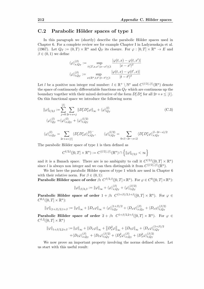
212 Appendix C. Holder spaces
C.2 Parabolic Holder spaces of type 1
In this paragraph we (shortly) describe the parabolic Holder spaces used inChapter 6. For a complete review see for example Chapter I in Ladyzenskaja et al.(1967). Let QT := (0, T ) × Rn and QT its closure. For ϕ : [0, T ] × Rn → E andβ ∈ (0, 1) we define
〈ϕ〉(β)x,QT
:= supt≤T,x,x′:|x−x′|≤1
|ϕ(t, x)− ϕ(t, x′)||x− x′|β
〈ϕ〉(β)t,QT
:= supx∈Rn,t,t′:|t−t′|≤1
|ϕ(t, x)− ϕ(t′, x)||t− t′|β
Let l be a positive non integer real number: l ∈ R+ \ N∗ and Cbl/2c,blc(Rn) denotethe space of continuously differentiable functions on QT which are continuous up theboundary together with their mixed derivative of the form Dr
tDsx for all 2r+s ≤ blc.
On this functional space we introduce the following norm
‖ϕ‖l/2,l :=
blc∑j=0
∑2r+s=j
‖DrtD
sxϕ‖∞ + 〈ϕ〉(l)QT (C.3)
〈ϕ〉(l)QT =〈ϕ〉(l)x,QT + 〈ϕ〉(l/2)t,QT
〈ϕ〉(l)x,QT =∑
2r+s=blc
〈DrtD
sxϕ〉l−x,QT
, 〈ϕ〉(l/2)t,QT
=∑
0<l−2r−s<2
〈DrtD
sxϕ〉
(l−2r−s)/2x,QT
The parabolic Holder space of type 1 is then defined as
C l/2,l([0, T ]× Rn) := Cbl/2c,blc(Rn) ∩‖ϕ‖l/2,l <∞
and it is a Banach space. There are is no ambiguity to call it C l/2,l([0, T ] × Rn)since l is always non integer and we can then distinguish it from Cbl/2c,blc(Rn).
We list here the parabolic Holder spaces of type 1 which are used in Chapter 6with their relative norm. For β ∈ (0, 1):Parabolic Holder space of order β: Cβ/2,β([0, T ]×Rn). For ϕ ∈ C0([0, T ]×Rn):
‖ϕ‖β/2,β := ‖ϕ‖∞ + 〈ϕ〉(β)x,QT
+ 〈ϕ〉(β/2)t,QT
Parabolic Holder space of order 1 + β: C(1+β)/2,1+β([0, T ] × Rn). For ϕ ∈C0,1([0, T ]× Rn):
‖ϕ‖(1+β)/2,1+β := ‖ϕ‖∞ + ‖Dxϕ‖∞ + 〈ϕ〉(1+β)/2t,QT
+ 〈Dxϕ〉(β)x,QT
+ 〈Dxϕ〉(β/2)t,QT
Parabolic Holder space of order 2 + β: C1+β/2,2+β([0, T ] × Rn). For ϕ ∈C1,2([0, T ]× Rn)
‖ϕ‖1+β/2,2+β := ‖ϕ‖∞ + ‖Dxϕ‖∞ +∥∥D2
xϕ∥∥∞ + ‖Dtϕ‖∞ + 〈Dxϕ〉(1+β)/2
t,QT
+〈Dtϕ〉(β)x,QT
+ 〈Dtϕ〉(β/2)t,QT
+ 〈D2xϕ〉
(β)x,QT
+ 〈D2xϕ〉
(β/2)t,QT
We now prove an important property involving the norms defined above. Letus start with this useful result:
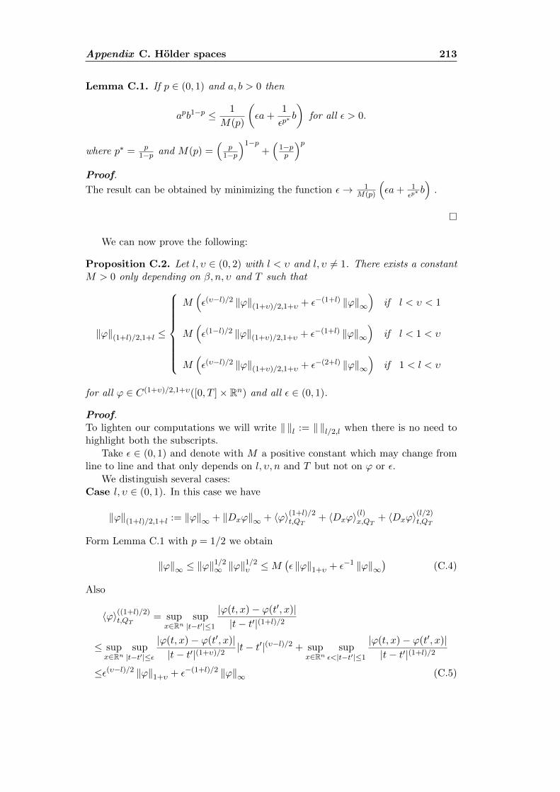
Appendix C. Holder spaces 213
Lemma C.1. If p ∈ (0, 1) and a, b > 0 then
apb1−p ≤ 1
M(p)
(εa+
1
εp∗b
)for all ε > 0.
where p∗ = p1−p and M(p) =
(p
1−p
)1−p+(
1−pp
)pProof.
The result can be obtained by minimizing the function ε→ 1M(p)
(εa+ 1
εp∗b)
.
We can now prove the following:
Proposition C.2. Let l, υ ∈ (0, 2) with l < υ and l, υ 6= 1. There exists a constantM > 0 only depending on β, n, υ and T such that
‖ϕ‖(1+l)/2,1+l ≤
M(ε(υ−l)/2 ‖ϕ‖(1+υ)/2,1+υ + ε−(1+l) ‖ϕ‖∞
)if l < υ < 1
M(ε(1−l)/2 ‖ϕ‖(1+υ)/2,1+υ + ε−(1+l) ‖ϕ‖∞
)if l < 1 < υ
M(ε(υ−l)/2 ‖ϕ‖(1+υ)/2,1+υ + ε−(2+l) ‖ϕ‖∞
)if 1 < l < υ
for all ϕ ∈ C(1+υ)/2,1+υ([0, T ]× Rn) and all ε ∈ (0, 1).
Proof.To lighten our computations we will write ‖ ‖l := ‖ ‖l/2,l when there is no need tohighlight both the subscripts.
Take ε ∈ (0, 1) and denote with M a positive constant which may change fromline to line and that only depends on l, υ, n and T but not on ϕ or ε.
We distinguish several cases:Case l, υ ∈ (0, 1). In this case we have
‖ϕ‖(1+l)/2,1+l := ‖ϕ‖∞ + ‖Dxϕ‖∞ + 〈ϕ〉(1+l)/2t,QT
+ 〈Dxϕ〉(l)x,QT + 〈Dxϕ〉(l/2)t,QT
Form Lemma C.1 with p = 1/2 we obtain
‖ϕ‖∞ ≤ ‖ϕ‖1/2∞ ‖ϕ‖
1/2υ ≤M
(ε ‖ϕ‖1+υ + ε−1 ‖ϕ‖∞
)(C.4)
Also
〈ϕ〉((1+l)/2)t,QT
= supx∈Rn
sup|t−t′|≤1
|ϕ(t, x)− ϕ(t′, x)||t− t′|(1+l)/2
≤ supx∈Rn
sup|t−t′|≤ε
|ϕ(t, x)− ϕ(t′, x)||t− t′|(1+υ)/2
|t− t′|(υ−l)/2 + supx∈Rn
supε<|t−t′|≤1
|ϕ(t, x)− ϕ(t′, x)||t− t′|(1+l)/2
≤ε(υ−l)/2 ‖ϕ‖1+υ + ε−(1+l)/2 ‖ϕ‖∞ (C.5)
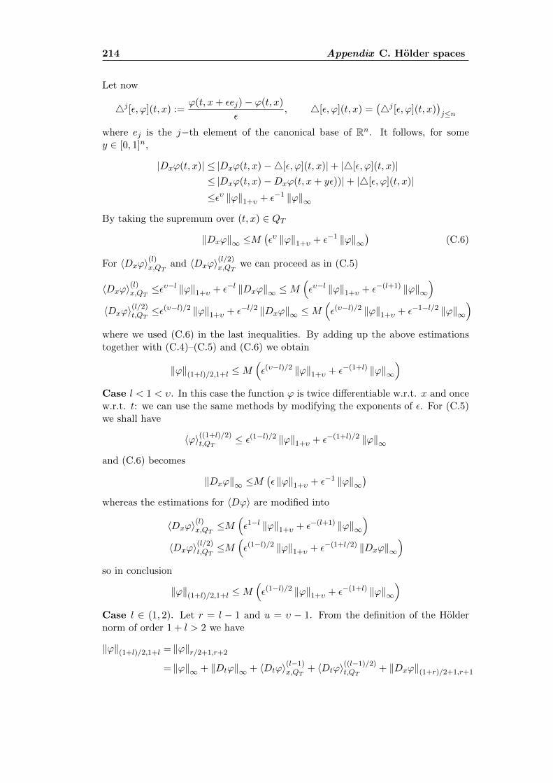
214 Appendix C. Holder spaces
Let now
4j [ε, ϕ](t, x) :=ϕ(t, x+ εej)− ϕ(t, x)
ε, 4[ε, ϕ](t, x) =
(4j [ε, ϕ](t, x)
)j≤n
where ej is the j−th element of the canonical base of Rn. It follows, for somey ∈ [0, 1]n,
|Dxϕ(t, x)| ≤ |Dxϕ(t, x)−4[ε, ϕ](t, x)|+ |4[ε, ϕ](t, x)|≤ |Dxϕ(t, x)−Dxϕ(t, x+ yε))|+ |4[ε, ϕ](t, x)|≤ευ ‖ϕ‖1+υ + ε−1 ‖ϕ‖∞
By taking the supremum over (t, x) ∈ QT
‖Dxϕ‖∞ ≤M(ευ ‖ϕ‖1+υ + ε−1 ‖ϕ‖∞
)(C.6)
For 〈Dxϕ〉(l)x,QT and 〈Dxϕ〉(l/2)x,QT
we can proceed as in (C.5)
〈Dxϕ〉(l)x,QT ≤ευ−l ‖ϕ‖1+υ + ε−l ‖Dxϕ‖∞ ≤M
(ευ−l ‖ϕ‖1+υ + ε−(l+1) ‖ϕ‖∞
)〈Dxϕ〉(l/2)
t,QT≤ε(υ−l)/2 ‖ϕ‖1+υ + ε−l/2 ‖Dxϕ‖∞ ≤M
(ε(υ−l)/2 ‖ϕ‖1+υ + ε−1−l/2 ‖ϕ‖∞
)where we used (C.6) in the last inequalities. By adding up the above estimationstogether with (C.4)–(C.5) and (C.6) we obtain
‖ϕ‖(1+l)/2,1+l ≤M(ε(υ−l)/2 ‖ϕ‖1+υ + ε−(1+l) ‖ϕ‖∞
)Case l < 1 < υ. In this case the function ϕ is twice differentiable w.r.t. x and oncew.r.t. t: we can use the same methods by modifying the exponents of ε. For (C.5)we shall have
〈ϕ〉((1+l)/2)t,QT
≤ ε(1−l)/2 ‖ϕ‖1+υ + ε−(1+l)/2 ‖ϕ‖∞
and (C.6) becomes
‖Dxϕ‖∞ ≤M(ε ‖ϕ‖1+υ + ε−1 ‖ϕ‖∞
)whereas the estimations for 〈Dϕ〉 are modified into
〈Dxϕ〉(l)x,QT ≤M(ε1−l ‖ϕ‖1+υ + ε−(l+1) ‖ϕ‖∞
)〈Dxϕ〉(l/2)
t,QT≤M
(ε(1−l)/2 ‖ϕ‖1+υ + ε−(1+l/2) ‖Dxϕ‖∞
)so in conclusion
‖ϕ‖(1+l)/2,1+l ≤M(ε(1−l)/2 ‖ϕ‖1+υ + ε−(1+l) ‖ϕ‖∞
)Case l ∈ (1, 2). Let r = l − 1 and u = υ − 1. From the definition of the Holdernorm of order 1 + l > 2 we have
‖ϕ‖(1+l)/2,1+l = ‖ϕ‖r/2+1,r+2
= ‖ϕ‖∞ + ‖Dtϕ‖∞ + 〈Dtϕ〉(l−1)x,QT
+ 〈Dtϕ〉((l−1)/2)t,QT
+ ‖Dxϕ‖(1+r)/2+1,r+1
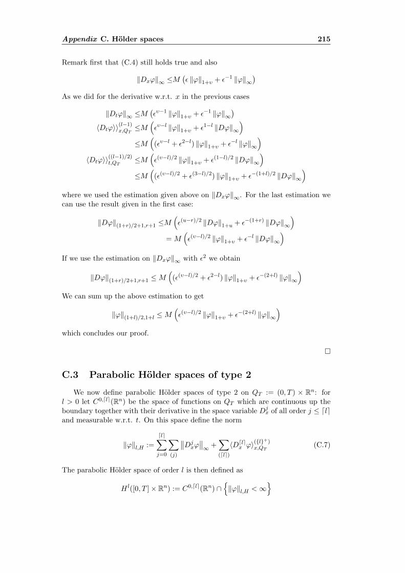
Appendix C. Holder spaces 215
Remark first that (C.4) still holds true and also
‖Dxϕ‖∞ ≤M(ε ‖ϕ‖1+υ + ε−1 ‖ϕ‖∞
)As we did for the derivative w.r.t. x in the previous cases
‖Dtϕ‖∞ ≤M(ευ−1 ‖ϕ‖1+υ + ε−1 ‖ϕ‖∞
)〈Dtϕ〉〉(l−1)
x,QT≤M
(ευ−l ‖ϕ‖1+υ + ε1−l ‖Dϕ‖∞
)≤M
((ευ−l + ε2−l) ‖ϕ‖1+υ + ε−l ‖ϕ‖∞
)〈Dtϕ〉〉((l−1)/2)
t,QT≤M
(ε(υ−l)/2 ‖ϕ‖1+υ + ε(1−l)/2 ‖Dϕ‖∞
)≤M
((ε(υ−l)/2 + ε(3−l)/2) ‖ϕ‖1+υ + ε−(1+l)/2 ‖Dϕ‖∞
)where we used the estimation given above on ‖Dxϕ‖∞. For the last estimation wecan use the result given in the first case:
‖Dϕ‖(1+r)/2+1,r+1 ≤M(ε(u−r)/2 ‖Dϕ‖1+u + ε−(1+r) ‖Dϕ‖∞
)= M
(ε(υ−l)/2 ‖ϕ‖1+υ + ε−l ‖Dϕ‖∞
)If we use the estimation on ‖Dxϕ‖∞ with ε2 we obtain
‖Dϕ‖(1+r)/2+1,r+1 ≤M(
(ε(υ−l)/2 + ε2−l) ‖ϕ‖1+υ + ε−(2+l) ‖ϕ‖∞)
We can sum up the above estimation to get
‖ϕ‖(1+l)/2,1+l ≤M(ε(υ−l)/2 ‖ϕ‖1+υ + ε−(2+l) ‖ϕ‖∞
)which concludes our proof.
C.3 Parabolic Holder spaces of type 2
We now define parabolic Holder spaces of type 2 on QT := (0, T ) × Rn: forl > 0 let C0,dle(Rn) be the space of functions on QT which are continuous up theboundary together with their derivative in the space variable Dj
x of all order j ≤ dleand measurable w.r.t. t. On this space define the norm
‖ϕ‖l,H :=
dle∑j=0
∑(j)
∥∥Djxϕ∥∥∞ +
∑(dle)
〈Ddlex ϕ〉(l+)
x,QT(C.7)
The parabolic Holder space of order l is then defined as
H l([0, T ]× Rn) := C0,dle(Rn) ∩‖ϕ‖l,H <∞
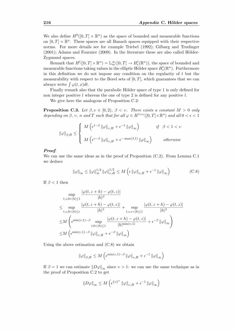
216 Appendix C. Holder spaces
We also define H0([0, T ] × Rn) as the space of bounded and measurable functionson [0, T ] × Rn. These spaces are all Banach spaces equipped with their respectivenorms. For more details see for example Triebel (1992); Gilbarg and Trudinger(2001); Adams and Fournier (2009). In the literature these are also called Holder-Zygmund spaces.
Remark that H l([0, T ]×Rn) = L∞m ([0, T ]→ H le(Rn)), the space of bounded and
measurable functions taking values in the elliptic Holder spaceH le(Rn). Furthermore
in this definition we do not impose any condition on the regularity of t but themeasurability with respect to the Borel sets of [0, T ], which guarantees that we canalways write
∫ϕ(t, x)dt.
Finally remark also that the parabolic Holder space of type 1 is only defined fornon integer positive l whereas the one of type 2 is defined for any positive l.
We give here the analogous of Proposition C.2:
Proposition C.3. Let β, υ ∈ [0, 2), β < υ. There exists a constant M > 0 onlydepending on β, υ, n and T such that for all ϕ ∈ H1+υ([0, T ]×Rn) and all 0 < ε < 1
‖ϕ‖β,H ≤
M(ε1−β ‖ϕ‖υ,H + ε−1 ‖ϕ‖∞
)if β < 1 < υ
M(ευ−β ‖ϕ‖υ,H + ε−max(β,1) ‖ϕ‖∞
)otherwise
Proof.We can use the same ideas as in the proof of Proposition (C.2). From Lemma C.1we deduce
‖ϕ‖∞ ≤ ‖ϕ‖1/2∞ ‖ϕ‖
1/2υ,H ≤M
(ε ‖ϕ‖υ,H + ε−1 ‖ϕ‖∞
)(C.8)
If β < 1 then
supt,z,0<|h|≤1
|ϕ(t, z + h)− ϕ(t, z)||h|β
≤ supt,z,0<|h|≤ε
|ϕ(t, z + h)− ϕ(t, z)||h|β
+ supt,z,ε<|h|≤1
|ϕ(t, z + h)− ϕ(t, z)||h|β
≤M
(εmin(υ,1)−β sup
t,0<|h|≤1
|ϕ(t, z + h)− ϕ(t, z)||h|min(υ,1)
+ ε−β ‖ϕ‖∞
)≤M
(εmin(υ,1)−β ‖ϕ‖υ,H + ε−β ‖ϕ‖∞
)Using the above estimation and (C.8) we obtain
‖ϕ‖β,H ≤M(εmin(υ,1)−β ‖ϕ‖υ,H + ε−1 ‖ϕ‖∞
)If β = 1 we can estimate ‖Dϕ‖∞ since υ > 1: we can use the same technique as inthe proof of Proposition C.2 to get
‖Dϕ‖∞ ≤M(ευ
+ ‖ϕ‖υ,H + ε−1 ‖ϕ‖∞)

Appendix C. Holder spaces 217
and then again
‖ϕ‖1,H ≤M(ευ−1 ‖ϕ‖υ,H + ε−1 ‖ϕ‖∞
)since υ+ = υ − 1. Finally if β > 1 we can repeat the argument as in the caseβ < 1:
〈Dϕ〉(β−1)z,QT
≤M(ευ−β ‖ϕ‖υ,H + ε1−β ‖Dϕ‖∞
)≤M
(ευ−β ‖ϕ‖υ,H + ε−β ‖ϕ‖∞
)by using the estimation on ‖Dϕ‖∞ so then
‖ϕ‖β,H ≤M(ευ−β ‖ϕ‖υ,H + ε−β ‖ϕ‖∞
)which concludes our proof.

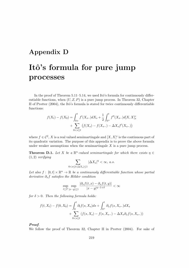
Appendix D
Ito’s formula for pure jumpprocesses
In the proof of Theorem 5.11–5.14, we used Ito’s formula for continuously differ-entiable functions, when (U,Z, P ) is a pure jump process. In Theorem 32, ChapterII of Protter (2004), the Ito’s formula is stated for twice continuously differentiablefunctions:
f(Xt)− f(X0) =
∫ t
0+f ′(Xs−)dXs +
1
2
∫ t
0+f ′′(Xs−)d[X,X]cs
+∑
0<s≤t
(f(Xs)− f(Xs−)−∆Xsf
′(Xs−))
where f ∈ C2, X is a real valued semimartingale and [X,X]c is the continuous part ofits quadratic variation. The purpose of this appendix is to prove the above formulaunder weaker assumptions when the semimartingale X is a pure jump process.
Theorem D.1. Let X be a Rn-valued semimartingale for which there exists η ∈(1, 2) verifying ∑
0<s≤t:|∆Xs|≤1
|∆Xs|η <∞, a.s.
Let also f : [0, t] × Rn → R be a continuously differentiable function whose partialderivative ∂xf satisfies the Holder condition
supt≤T
sup|x−y|≤1
|∂xf(t, x)− ∂xf(t, y)||x− y|η−1+δ
<∞
for δ > 0. Then the following formula holds:
f(t,Xt)− f(0, X0) =
∫ t
0∂tf(s,Xs)ds+
∫ t
0+∂xf(s,Xs−)dXs
+∑
0<s≤t(f(s,Xs)− f(s,Xs−)−∆Xs∂xf(s,Xs−))
Proof.We follow the proof of Theorem 32, Chapter II in Protter (2004). For sake of
219
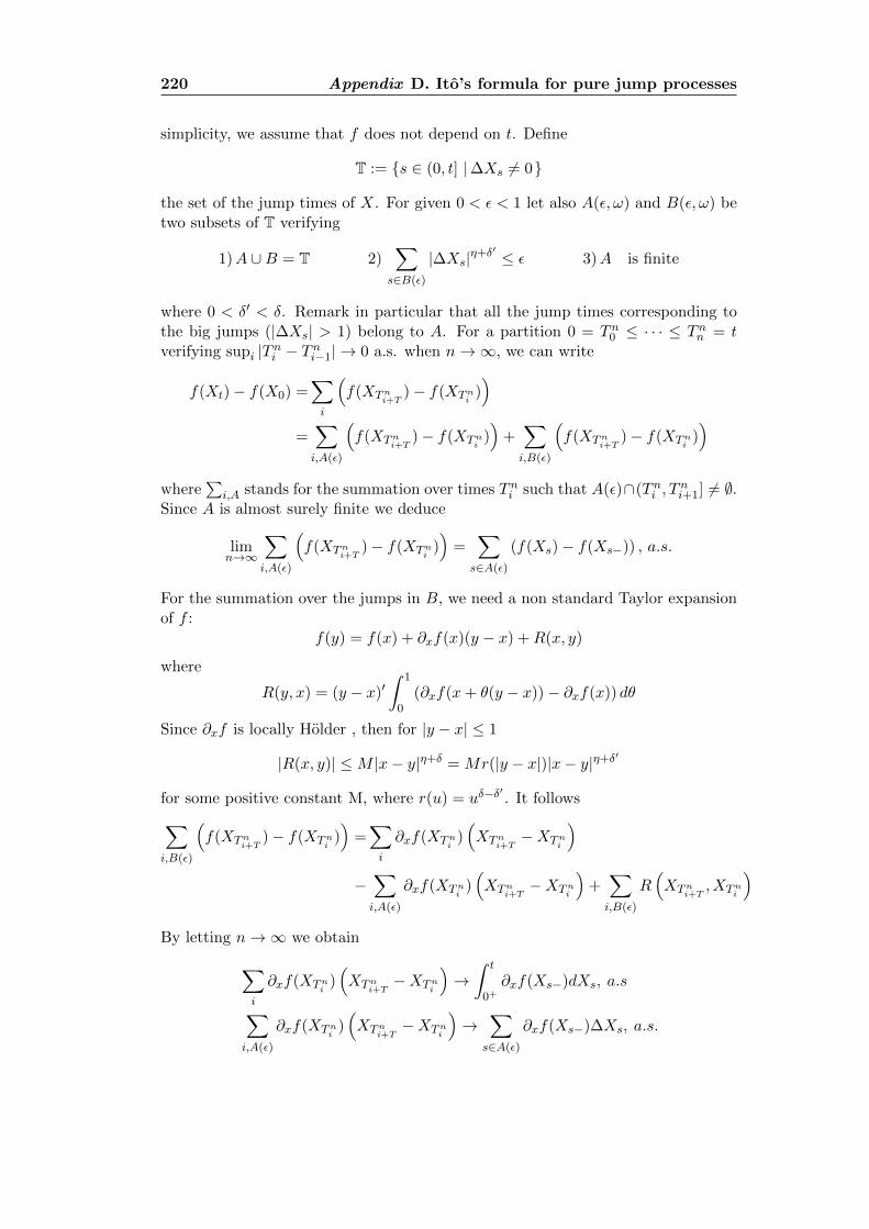
220 Appendix D. Ito’s formula for pure jump processes
simplicity, we assume that f does not depend on t. Define
T := s ∈ (0, t] |∆Xs 6= 0
the set of the jump times of X. For given 0 < ε < 1 let also A(ε, ω) and B(ε, ω) betwo subsets of T verifying
1)A ∪B = T 2)∑s∈B(ε)
|∆Xs|η+δ′ ≤ ε 3)A is finite
where 0 < δ′ < δ. Remark in particular that all the jump times corresponding tothe big jumps (|∆Xs| > 1) belong to A. For a partition 0 = Tn0 ≤ · · · ≤ Tnn = tverifying supi |Tni − Tni−1| → 0 a.s. when n→∞, we can write
f(Xt)− f(X0) =∑i
(f(XTni+T
)− f(XTni))
=∑i,A(ε)
(f(XTni+T
)− f(XTni))
+∑i,B(ε)
(f(XTni+T
)− f(XTni))
where∑
i,A stands for the summation over times Tni such that A(ε)∩(Tni , Tni+1] 6= ∅.
Since A is almost surely finite we deduce
limn→∞
∑i,A(ε)
(f(XTni+T
)− f(XTni))
=∑s∈A(ε)
(f(Xs)− f(Xs−)) , a.s.
For the summation over the jumps in B, we need a non standard Taylor expansionof f :
f(y) = f(x) + ∂xf(x)(y − x) +R(x, y)
where
R(y, x) = (y − x)′∫ 1
0(∂xf(x+ θ(y − x))− ∂xf(x)) dθ
Since ∂xf is locally Holder , then for |y − x| ≤ 1
|R(x, y)| ≤M |x− y|η+δ = Mr(|y − x|)|x− y|η+δ′
for some positive constant M, where r(u) = uδ−δ′. It follows∑
i,B(ε)
(f(XTni+T
)− f(XTni))
=∑i
∂xf(XTni)(XTni+T
−XTni
)−∑i,A(ε)
∂xf(XTni)(XTni+T
−XTni
)+∑i,B(ε)
R(XTni+T
, XTni
)By letting n→∞ we obtain∑
i
∂xf(XTni)(XTni+T
−XTni
)→∫ t
0+∂xf(Xs−)dXs, a.s∑
i,A(ε)
∂xf(XTni)(XTni+T
−XTni
)→
∑s∈A(ε)
∂xf(Xs−)∆Xs, a.s.
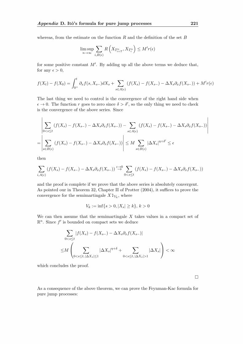
Appendix D. Ito’s formula for pure jump processes 221
whereas, from the estimate on the function R and the definition of the set B
lim supn→∞
∑i,B(ε)
R(XTni+T
, XTni
)≤M ′r(ε)
for some positive constant M ′. By adding up all the above terms we deduce that,for any ε > 0,
f(Xt)− f(X0) =
∫ t
0+∂xf(s,Xs−)dXs +
∑s∈A(ε)
(f(Xs)− f(Xs−)−∆Xs∂xf(Xs−)) +M ′r(ε)
The last thing we need to control is the convergence of the right hand side whenε→ 0. The function r goes to zero since δ > δ′, so the only thing we need to checkis the convergence of the above series. Since∣∣∣∣∣∣
∑0<s≤t
(f(Xs)− f(Xs−)−∆Xs∂xf(Xs−))−∑s∈A(ε)
(f(Xs)− f(Xs−)−∆Xs∂xf(Xs−))
∣∣∣∣∣∣=
∣∣∣∣∣∣∑s∈B(ε)
(f(Xs)− f(Xs−)−∆Xs∂xf(Xs−))
∣∣∣∣∣∣ ≤M∑s∈B(ε)
|∆Xs|η+δ′ ≤ ε
then∑i,A(ε)
(f(Xs)− f(Xs−)−∆Xs∂xf(Xs−))ε→0→
∑0<s≤t
(f(Xs)− f(Xs−)−∆Xs∂xf(Xs−))
and the proof is complete if we prove that the above series is absolutely convergent.As pointed our in Theorem 32, Chapter II of Protter (2004), it suffices to prove theconvergence for the semimartingale X1Vk , where
Vk := infs > 0, |Xs| ≥ k, k > 0
We can then assume that the semimartingale X takes values in a compact set ofRn. Since f ′ is bounded on compact sets we deduce∑
0<s≤t|f(Xs)− f(Xs−)−∆Xs∂xf(Xs−)|
≤M
∑0<s≤t, |∆Xs|≤1
|∆Xs|η+δ +∑
0<s≤t, |∆Xs|>1
|∆Xs|
<∞
which concludes the proof.
As a consequence of the above theorem, we can prove the Feynman-Kac formula forpure jump processes:
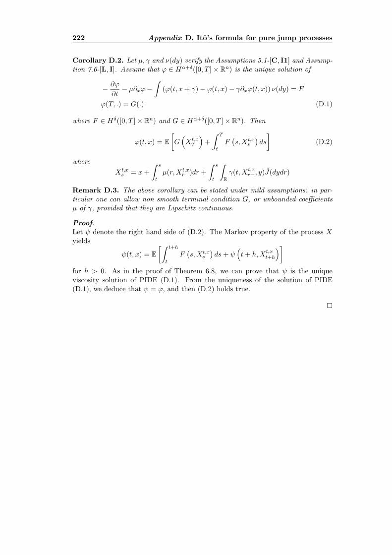
222 Appendix D. Ito’s formula for pure jump processes
Corollary D.2. Let µ, γ and ν(dy) verify the Assumptions 5.1-[C, I1] and Assump-tion 7.6-[L, I]. Assume that ϕ ∈ Hα+δ([0, T ]× Rn) is the unique solution of
− ∂ϕ
∂t− µ∂xϕ−
∫(ϕ(t, x+ γ)− ϕ(t, x)− γ∂xϕ(t, x)) ν(dy) = F
ϕ(T, .) = G(.) (D.1)
where F ∈ Hδ([0, T ]× Rn) and G ∈ Hα+δ([0, T ]× Rn). Then
ϕ(t, x) = E[G(Xt,xT
)+
∫ T
tF(s,Xt,x
s
)ds
](D.2)
where
Xt,xs = x+
∫ s
tµ(r,Xt,x
r )dr +
∫ s
t
∫Rγ(t,Xt,x
r−, y)J(dydr)
Remark D.3. The above corollary can be stated under mild assumptions: in par-ticular one can allow non smooth terminal condition G, or unbounded coefficientsµ of γ, provided that they are Lipschitz continuous.
Proof.Let ψ denote the right hand side of (D.2). The Markov property of the process Xyields
ψ(t, x) = E[∫ t+h
tF(s,Xt,x
s
)ds+ ψ
(t+ h,Xt,x
t+h
)]for h > 0. As in the proof of Theorem 6.8, we can prove that ψ is the uniqueviscosity solution of PIDE (D.1). From the uniqueness of the solution of PIDE(D.1), we deduce that ψ = ϕ, and then (D.2) holds true.
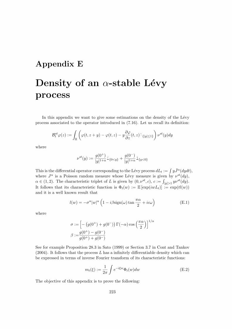
Appendix E
Density of an α-stable Levyprocess
In this appendix we want to give some estimations on the density of the Levyprocess associated to the operator introduced in (7.16). Let us recall its definition:
Bstt ϕ(z) :=
∫R
(ϕ(t, z + y)− ϕ(t, z)− y∂ϕ
∂z(t, z)1|y|≤1
)νst(y)dy
where
νst(y) :=g(0+)
|y|1+α10<y +
g(0−)
|y|1+α1y<0
This is the differential operator corresponding to the Levy process dLt :=∫yJα(dydt),
where Jα is a Poisson random measure whose Levy measure is given by νst(dy),α ∈ (1, 2). The characteristic triplet of L is given by (0, νst, c), c :=
∫|y|>1 yν
st(dy).
It follows that its characteristic function is Φt(w) := E [exp(iwLt)] := exp(tl(w))and it is a well known result that
l(w) = −σα|w|α(
1− iβsign(ω) tanπα
2+ icω
)(E.1)
where
σ :=[−(g(0+) + g(0−)
)Γ(−α) cos
(πα2
)]1/α
β :=g(0+)− g(0−)
g(0+) + g(0−)
See for example Proposition 28.3 in Sato (1999) or Section 3.7 in Cont and Tankov(2004). It follows that the process L has a infinitely differentiable density which canbe expressed in terms of inverse Fourier transform of its characteristic functions:
mt(ξ) :=1
2π
∫e−iξwΦt(w)dw (E.2)
The objective of this appendix is to prove the following:
223
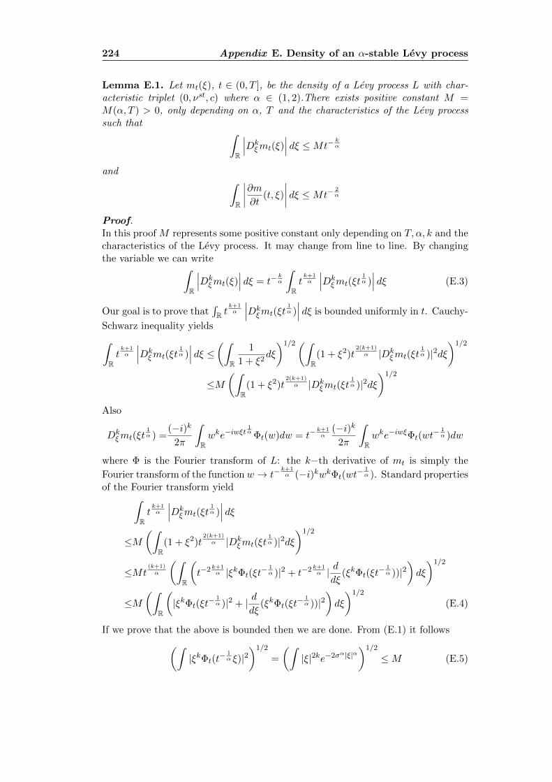
224 Appendix E. Density of an α-stable Levy process
Lemma E.1. Let mt(ξ), t ∈ (0, T ], be the density of a Levy process L with char-acteristic triplet (0, νst, c) where α ∈ (1, 2).There exists positive constant M =M(α, T ) > 0, only depending on α, T and the characteristics of the Levy processsuch that ∫
R
∣∣∣Dkξmt(ξ)
∣∣∣ dξ ≤Mt−kα
and ∫R
∣∣∣∣∂m∂t (t, ξ)
∣∣∣∣ dξ ≤Mt−2α
Proof.In this proof M represents some positive constant only depending on T, α, k and thecharacteristics of the Levy process. It may change from line to line. By changingthe variable we can write∫
R
∣∣∣Dkξmt(ξ)
∣∣∣ dξ = t−kα
∫Rtk+1α
∣∣∣Dkξmt(ξt
1α )∣∣∣ dξ (E.3)
Our goal is to prove that∫R t
k+1α
∣∣∣Dkξmt(ξt
1α )∣∣∣ dξ is bounded uniformly in t. Cauchy-
Schwarz inequality yields∫Rtk+1α
∣∣∣Dkξmt(ξt
1α )∣∣∣ dξ ≤(∫
R
1
1 + ξ2dξ
)1/2(∫R
(1 + ξ2)t2(k+1)α |Dk
ξmt(ξt1α )|2dξ
)1/2
≤M(∫
R(1 + ξ2)t
2(k+1)α |Dk
ξmt(ξt1α )|2dξ
)1/2
Also
Dkξmt(ξt
1α ) =
(−i)k
2π
∫Rwke−iwξt
1α Φt(w)dw = t−
k+1α
(−i)k
2π
∫Rwke−iwξΦt(wt
− 1α )dw
where Φ is the Fourier transform of L: the k−th derivative of mt is simply the
Fourier transform of the function w → t−k+1α (−i)kwkΦt(wt
− 1α ). Standard properties
of the Fourier transform yield∫Rtk+1α
∣∣∣Dkξmt(ξt
1α )∣∣∣ dξ
≤M(∫
R(1 + ξ2)t
2(k+1)α |Dk
ξmt(ξt1α )|2dξ
)1/2
≤Mt(k+1)α
(∫R
(t−2 k+1
α |ξkΦt(ξt− 1α )|2 + t−2 k+1
α | ddξ
(ξkΦt(ξt− 1α ))|2
)dξ
)1/2
≤M(∫
R
(|ξkΦt(ξt
− 1α )|2 + | d
dξ(ξkΦt(ξt
− 1α ))|2
)dξ
)1/2
(E.4)
If we prove that the above is bounded then we are done. From (E.1) it follows(∫|ξkΦt(t
− 1α ξ)|2
)1/2
=
(∫|ξ|2ke−2σα|ξ|α
)1/2
≤M (E.5)

Appendix E. Density of an α-stable Levy process 225
For the second term, we first remark that
ξkΦt(ξt− 1α ) = ξk exp
(−σα|ξ|α
(1− iβ tan(
απ
2)sign(ξ)
)+ ict1−1/αξ
)from which we deduce
| ddξ
(ξkΦt(ξt− 1α ))| ≤M
(1 + ξk
)exp (−σα|ξ|α)
so then (∫| ddξ
(ξkΦt(ξt− 1α ))|2dξ
)1/2
≤M
since 1 < α < 2. We use the above estimations and (E.5) in (E.4) to prove the firstpart of the Lemma.
For the second part, we can remark that the density function of the Levy processLt,ls , ξ → m(s− t, ξ − l), verifies
∂m
∂t(s− t, ξ − l)
+
∫ (m(s− t, ξ − l − y)−m(s− t, ξ − l)− y∂m
∂ξ(s− t, ξ − l)1|y|≤1
)νst(dy) = 0,
m(0, ξ) = δl(ξ)
where δl(ξ) is the Dirac mass at the point l. It follows∣∣∣∣∂m∂t (t, ξ − l)∣∣∣∣ ≤1
2
∫|y|≤1
|y|2∫ 1
0dθ
∣∣∣∣∂2m
∂ξ2(t, ξ − l − θy)
∣∣∣∣ νst(dy)
+
∫|y|>1
|m(t, ξ − l − y)−m(t, ξ − l)| νst(dy)
We now integrate over ξ, and by using the previous estimate, we obtain∫R
∣∣∣∣∂m∂t (t, ξ)
∣∣∣∣ dξ ≤Mt−2α

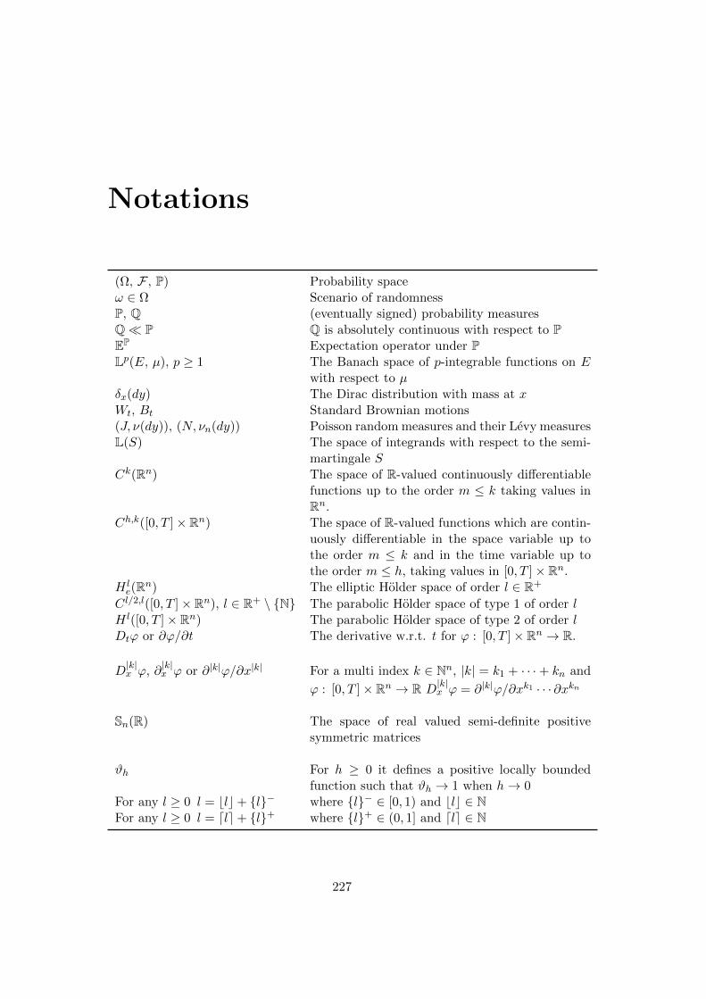
Notations
(Ω, F , P) Probability spaceω ∈ Ω Scenario of randomnessP, Q (eventually signed) probability measuresQ P Q is absolutely continuous with respect to PEP Expectation operator under PLp(E, µ), p ≥ 1 The Banach space of p-integrable functions on E
with respect to µδx(dy) The Dirac distribution with mass at xWt, Bt Standard Brownian motions(J, ν(dy)), (N, νn(dy)) Poisson random measures and their Levy measuresL(S) The space of integrands with respect to the semi-
martingale SCk(Rn) The space of R-valued continuously differentiable
functions up to the order m ≤ k taking values inRn.
Ch,k([0, T ]× Rn) The space of R-valued functions which are contin-uously differentiable in the space variable up tothe order m ≤ k and in the time variable up tothe order m ≤ h, taking values in [0, T ]× Rn.
H le(Rn) The elliptic Holder space of order l ∈ R+
C l/2,l([0, T ]× Rn), l ∈ R+ \ N The parabolic Holder space of type 1 of order lH l([0, T ]× Rn) The parabolic Holder space of type 2 of order lDtϕ or ∂ϕ/∂t The derivative w.r.t. t for ϕ : [0, T ]× Rn → R.
D|k|x ϕ, ∂
|k|x ϕ or ∂|k|ϕ/∂x|k| For a multi index k ∈ Nn, |k| = k1 + · · ·+ kn and
ϕ : [0, T ]× Rn → R D|k|x ϕ = ∂|k|ϕ/∂xk1 · · · ∂xkn
Sn(R) The space of real valued semi-definite positivesymmetric matrices
ϑh For h ≥ 0 it defines a positive locally boundedfunction such that ϑh → 1 when h→ 0
For any l ≥ 0 l = blc+ l− where l− ∈ [0, 1) and blc ∈ NFor any l ≥ 0 l = dle+ l+ where l+ ∈ (0, 1] and dle ∈ N
227

Index
Acceptance set, 33
BSDEs with jumps, 115
Copulae, 57CVaR, 36, 60
Density of a α-stable Levy process, 223Derivative of flow, 85, 203Dirichlet boundary condition, 178, 183Doleans-Dade Exponential, 199Dynamic programming principle, 98
Electricity markets, 155Entropy, 37, 51
Future contracts, 158
G-divergence, 37, 61Galtchouk-Kunita-Watanabe decomposi-
tion, 68Generalized inverse distribution, 35, 56Green’s function, 187
Holder spaces, 211Hitting time, 189
Linear PDE fundamental solution, 106
Normal Inverse Gaussian process, 22, 171
Optimal quadratic hedge price, 89, 96
Portfolio insurance, 40, 63Pure investment problem, 69, 73, 74, 124,
147, 179
Quadratic hedge, 68
Risk measures, 31, 41spectral, 35coherent, 33continuous from above, 34
continuous from below, 34convex, 33law invariant, 32, 40minimal penalty function, 34, 45, 51on Lp spaces, 38representation, 33spectral, 36, 56
Sobolev space, 116
Utility-based hedging, 68
VaR, 35Variance-optimal signed martingale mea-
sure, 74Viscosity solution, 96, 140, 150, 183, 191
229

Bibliography
Adams, R. and J. Fournier (2009). Sobolev spaces, II edition, Volume 65. Academicpress New York.
Artzner, P., F. Delbaen, J. Eber, and D. Heath (1999). Coherent measures of risk.Mathematical finance 9 (3), 203–228.
Ash, R. and C. Doleans-Dade (2000). Probability and measure theory. AcademicPress.
Barles, G., R. Buckdahn, and E. Pardoux (1997). Backward stochastic differentialequations and integral-partial differential equations. Stochastics: An Interna-tional Journal of Probability and Stochastic Processes 60 (1-2), 57–83.
Barles, G., E. Chasseigne, and C. Imbert (2008). The dirichlet problem for second-order elliptic integro-differential equations. Indiana University Mathematics Jour-nal 57 (1), 213–146.
Barles, G. and C. Imbert (2008). Second-order elliptic integro-differential equations:viscosity solutions’ theory revisited. 25 (3), 567–585.
Barrieu, P. and N. El Karoui (2004). Optimal derivatives design under dynamicrisk measures. 351, 13.
Barrieu, P. and N. El Karoui (2008). Pricing, hedging and optimally designingderivatives via minimization of risk measures. Indifference Pricing , 77–141.
Basak, S. and A. Shapiro (2001). Value-at-risk-based risk management: optimalpolicies and asset prices. Review of Financial Studies 14 (2), 371.
Basel Committee(1996). Overview of the amendment to the capital accord to in-corporate market risks. www.bsi.org .
Basel Committee(2004). International convergence of capital measurement and cap-ital standards: a revised framework. www.bsi.org .
Bensoussan, A. and J. Lions (1984). Impulse control and quasi-variational inequal-ities, Volume 216. Gauthier-Villars Paris.
Biagini, S. and M. Frittelli (2009). On the extension of the namioka-klee theoremand on the fatou property for risk measures. Optimality and Risk-Modern Trendsin Mathematical Finance, 1–28.
231
232 Bibliography
Bion-Nadal, J. (2008). Dynamic risk measures: time consistency and risk measuresfrom bmo martingales. Finance and Stochastics 12 (2), 219–244.
Bion-Nadal, J. (2009). Time consistent dynamic risk processes. Stochastic Processesand their Applications 119 (2), 633–654.
Black, F. and A. Perold (1992). Theory of constant proportion portfolio insurance.Journal of Economic Dynamics and Control 16 (3-4), 403–426.
Bouchard, B., R. Elie, and C. Imbert (2010). Optimal control under stochastictarget constraints. SIAM Journal on Control and Optimization 48, 5.
Bouchard, B., R. Elie, and N. Touzi (2009). Stochastic target problems with con-trolled loss. SIAM Journal on Control and Optimization 48 (5), 3123–3150.
Boyle, P. and W. Tian (2007). Portfolio management with constraints. MathematicalFinance 17 (3), 319–343.
Cannarsa, P. and C. Sinestrari (2004). Semiconcave functions, Hamilton-Jacobiequations, and optimal control. Birkhauser.
Cerny, A. and J. Kallsen (2007). On the structure of general mean-variance hedgingstrategies. The Annals of probability 35 (4), 1479–1531.
Cerny, A. and J. Kallsen (2008). Mean–Variance Hedging and Optimal Investmentin Heston’s Model with Correlation. Mathematical Finance 18 (3), 473–492.
Clewlow, L. and C. Strickland (2000). Energy derivatives: pricing and risk man-agement, Volume 124. Lacima publications Warwick.
Cont, R. and P. Tankov (2004). Financial modelling with jump processes. Chapman& Hall.
Cont, R. and P. Tankov (2009). Constant proportion portfolio insurance in thepresence of jumps in asset prices. Mathematical Finance 19 (3), 379–401.
Cont, R., P. Tankov, and E. Voltchkova (2007). Hedging with options in modelswith jumps. Stochastic analysis and applications, 197–217.
Crandall, M., H. Ishii, and P. Lions (1992). User’s guide to viscosity solutions ofsecond order partial differential equations, Volume 27. American MathematicalSociety.
Crepey, S. and A. Matoussi (2008). Reflected and doubly reflected bsdes with jumps:a priori estimates and comparison. The Annals of Applied Probability 18 (5),2041–2069.
Csiszar, I. (1967). On topological properties of f-divergences. Studia Sci. Math.Hungarica 2, 329–339.
De Franco, C. and P. Tankov (2011). Portfolio insurance under a risk-measureconstraint. Insurance: Mathematics and Economics 49 (3), 361–370.
Bibliography 233
De Franco, C., P. Tankov, and X. Warin (2012). Quadratic hedge in electricitymarkets. working paper .
Delbaen, F., P. Grandits, T. Rheinlander, D. Samperi, M. Schweizer, and C. Stricker(2002). Exponential hedging and entropic penalties. Mathematical Finance 12 (2),99–123.
Doleans-Dade, C. (1970). Quelques applications de la formule de changement devariables pour les semimartingales. Probability Theory and Related Fields 16 (3),181–194.
Doob, J. (1994). Measure theory, Volume 143. Springer.
Ekeland, I., A. Galichon, and M. Henry (2009). Comonotonic measures of multi-variate risks. Mathematical Finance.
Ekeland, I. and W. Schachermayer (2011). Law invariant risk measures on Rn.Working paper .
El Karoui, N., M. Jeanblanc, and V. Lacoste (2005). Optimal portfolio manage-ment with american capital guarantee. Journal of Economic Dynamics and Con-trol 29 (3), 449–468.
El Karoui, N., S. Peng, and M. Quenez (1997). Backward stochastic differentialequations in finance. Mathematical finance 7 (1), 1–71.
El Karoui, N. and R. Rouge (2000). Pricing via utility maximization and entropy.Mathematical Finance 10 (2), 259–276.
Emmer, S., C. Kluppelberg, and R. Korn (2001). Optimal portfolios with boundedcapital at risk. Mathematical Finance 11 (4), 365–384.
Follmer, H. and P. Leukert (1999). Quantile hedging. Finance and Stochastics 3 (3),251–273.
Follmer, H. and A. Schied (2004). Stochastic finance. an introduction in discretetime. de Gruyter Studies in Mathematics, 648.
Forsyth, P., Y. d’Halluin, and K. Vetzal (2005). Robust numerical methods forcontingent claims under jump diffusion processes. IMA Journal of NumericalAnalysis 25 (1), 87–112.
Forsyth, P. and G. Labahn (2007). Numerical methods for controlled hamilton-jacobi-bellman pdes in finance. Journal of Computational Finance 11 (2).
Forsyth, P., J. Wan, and I. Wang (2007). Robust numerical valuation of euro-pean and american options under the cgmy process. Journal of ComputationalFinance 10 (4), 31.
Friedman, A. (1964). Partial differential equations of parabolic type, Volume 196.Prentice-Hall Englewood Cliffs, NJ.
234 Bibliography
Frittelli, M. and E. Gianin (2004). Dynamic convex risk measures. Risk measuresfor the 21st century , 227–248.
Galtchouk, L. (1976). Representation des martingales engendrees par un processusa accroissements independants (cas des martingales de carre integrable). Annalesde Henri Poincare (B) 12, 199–211.
Geman, H. and A. Roncoroni (2006). Understanding the fine structure of electricityprices. Journal of Business 79 (3).
Gilbarg, D. and N. Trudinger (2001). Elliptic partial differential equations of secondorder. Springer Verlag.
Gundel, A. and S. Weber (2007). Robust utility maximization with limited downsiderisk in incomplete markets. Stochastic Processes and Their Applications 117 (11),1663–1688.
He, X. and X. Zhou (2010). Portfolio choice via quantiles. Preprint .
Hubalek, F., J. Kallsen, and L. Krawczyk (2006). Variance-optimal hedging forprocesses with stationary independent increments. The Annals of Applied Prob-ability 16 (2), 853–885.
Ishii, H. (1989). On uniqueness and existence of viscosity solutions of fully nonlin-ear second-order elliptic pde’s. Communications on pure and applied mathemat-ics 42 (1), 15–45.
Jacod, J. and A. Shiryaev (2003). Limit Theorems for Stochastic Processes. Berlin:Springer.
Jakobsen, E. and K. Karlsen (2005). Continuous dependence estimates for viscositysolutions of integro-pdes. Journal of Differential Equations 212 (2), 278–318.
Jakobsen, E. and K. Karlsen (2006). A maximum principle for semicontinuousfunctions applicable to integro-partial differential equations. NoDEA: NonlinearDifferential Equations and Applications 13 (2), 137–165.
Jeanblanc, M., M. Mania, M. Santacroce, and M. Schweizer (2011). Mean-VarianceHedging via Stochastic Control and BSDEs for General Semimartingales. Work-ing paper .
Jensen, R. (1988). The maximum principle for viscosity solutions of fully nonlinearsecond order partial differential equations. Archive for Rational Mechanics andAnalysis 101 (1), 1–27.
Jin, H. and X. Yu Zhou (2008). Behavioral portfolio selection in continuous time.Mathematical Finance 18 (3), 385.
Jouini, E., M. Meddeb, and N. Touzi (2004). Vector-valued coherent risk measures.Finance and Stochastics 8 (4), 531–552.
Jouini, E., W. Schachermayer, and N. Touzi (2006). Law invariant risk measureshave the fatou property. Advances in mathematical economics, 49–71.
Bibliography 235
Kaina, M. and L. Ruschendorf (2009). On convex risk measures on lp-spaces. Math-ematical methods of operations research 69 (3), 475–495.
Kallsen, J. and R. Vierthauer (2009). Quadratic hedging in affine stochastic volatil-ity models. Review of Derivatives Research 12 (1), 3–27.
Karatzas, I. and S. Shreve (1998). Methods of mathematical finance. SpringerVerlag.
Kunita, H. and S. Watanabe (1967). On square integrable martingales. NagoyaMathematical Journal 30, 209–245.
Ladyzenskaja, O., V. Solonnikov, and N. Ural’ceva (1967). Linear and quasilinearequations of parabolic type, Translations of Mathematical Monographs, Vol. 23.
Laurent, J. and H. Pham (1999). Dynamic programming and mean-variance hedg-ing. Finance and Stochastics 3 (1), 83–110.
Liese, F. and I. Vajda (1987). Convex statistical distances. Teubner-Texte zurMathematik 95. Teubner Verlagsgesellschaft, Leipzig,.
Lions, P. (1983). Optimal control of diffusion processes and hamilton–jacobi–bellman equations. Communications in partial differential equations 8 (11), PartI 1101–1134, Part II 1229–1276.
Meyer-Brandis, T. and P. Tankov (2008). Multi-factor jump-diffusion models ofelectricity prices. International Journal of Theoretical and Applied Finance 11 (5),503–528.
Mikulevicius, R. and H. Pragarauskas (2009). On Holder solutions of the integro-differential Zakai equation. Stochastic Processes and their Applications 119 (10).
Mikulevicius, R. and H. Pragarauskas (2011). On the cauchy problem for inte-gro differential operators in Holder classes and the uniqueness of the martingaleproblem. preprint, arXiv:1103.3492.
Pham, H. (1998). Optimal stopping of controlled jump diffusion processes: a vis-cosity solution approach. Journal of Mathematical Systems, Estimation and Con-trol 8 (1), 1–27.
Pham, H. (2000). On quadratic hedging in continuous time. Mathematical Methodsof Operations Research 51 (2), 315–339.
Pham, H. (2007). Optimisation et controle stochastique appliques a la finance.Springer Verlag.
Protter, P. (2004). Stochastic integration and differential equations. Springer Verlag.
Rockafellar, R. and S. Uryasev (2000). Optimization of conditional value-at-risk.Journal of risk 2, 21–42.
Rogers, L. (2009). Optimal and robust contracts for a risk-constrained principal.Mathematics and Financial Economics 2 (3), 151–171.

236 Bibliography
Rong, S. (1997). On solutions of backward stochastic differential equations withjumps and applications. Stochastic Processes and their Applications 66 (2), 209–236.
Royer, M. (2006). Backward stochastic differential equations with jumps and re-lated non-linear expectations. Stochastic processes and their applications 116 (10),1358–1376.
Sato, K. (1999). Levy processes and infinitely divisible distributions. CambridgeUniv Pr.
Schweizer, M. (2001). A guided tour through quadratic hedging approaches . In:Option Pricing, Interest Rates and Risk Management (eds: Jouini E, Cvitanic Jand Musiela M), 538–574.
Triebel, H. (1992). Theory of function spaces II. Modern Birkhauser Classics.