Embed Size (px)
Citation preview
Two-Way ANOVA
Chapter 11
Golf anyone?
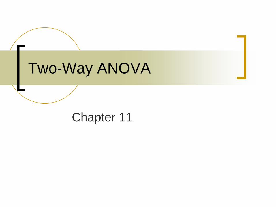
A sports psychologist is interest in comparing the
effects of two instructional methods on golf performance.
100 novice golfers (50 boys and 50 girls)
Method I Method II
65 55
IV: Method Type
DV: Golf proficiency
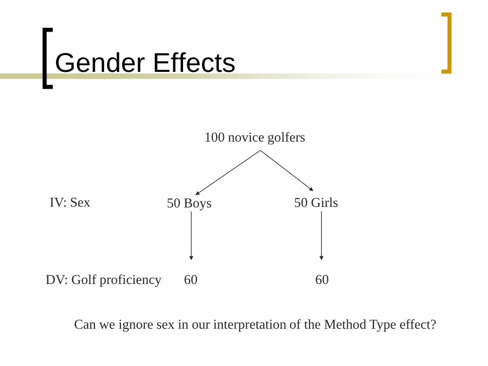
Gender Effects
100 novice golfers
50 Boys 50 Girls
60 60
IV: Sex
DV: Golf proficiency
Can we ignore sex in our interpretation of the Method Type effect?
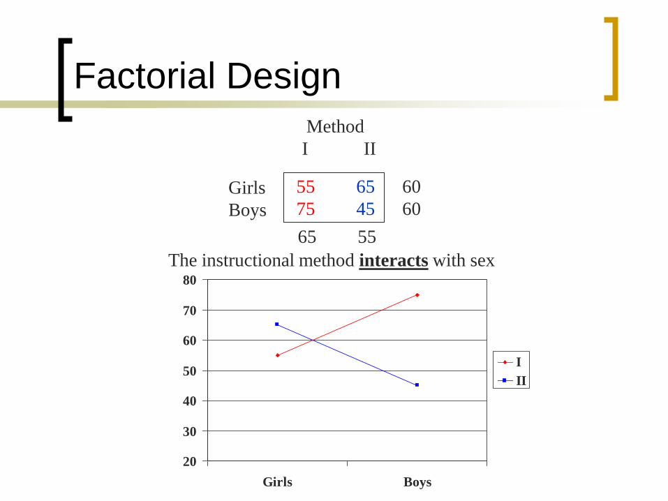
Factorial Design
Method
I II
65 55
60
60
Girls
Boys
55 65
75 45
20
30
40
50
60
70
80
Girls Boys
I
II
The instructional method interacts with sex
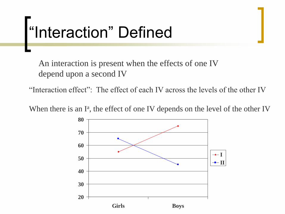
“Interaction” Defined
An interaction is present when the effects of one IV
depend upon a second IV
“Interaction effect”: The effect of each IV across the levels of the other IV
When there is an Ia, the effect of one IV depends on the level of the other IV
20
30
40
50
60
70
80
Girls Boys
I
II
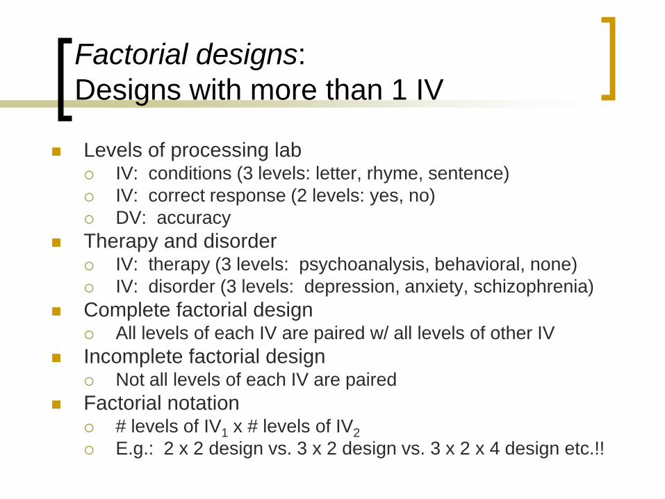
Factorial designs:
Designs with more than 1 IV
Levels of processing lab IV: conditions (3 levels: letter, rhyme, sentence)
IV: correct response (2 levels: yes, no)
DV: accuracy
Therapy and disorder IV: therapy (3 levels: psychoanalysis, behavioral, none)
IV: disorder (3 levels: depression, anxiety, schizophrenia)
Complete factorial design All levels of each IV are paired w/ all levels of other IV
Incomplete factorial design Not all levels of each IV are paired
Factorial notation # levels of IV1 x # levels of IV2
E.g.: 2 x 2 design vs. 3 x 2 design vs. 3 x 2 x 4 design etc.!!
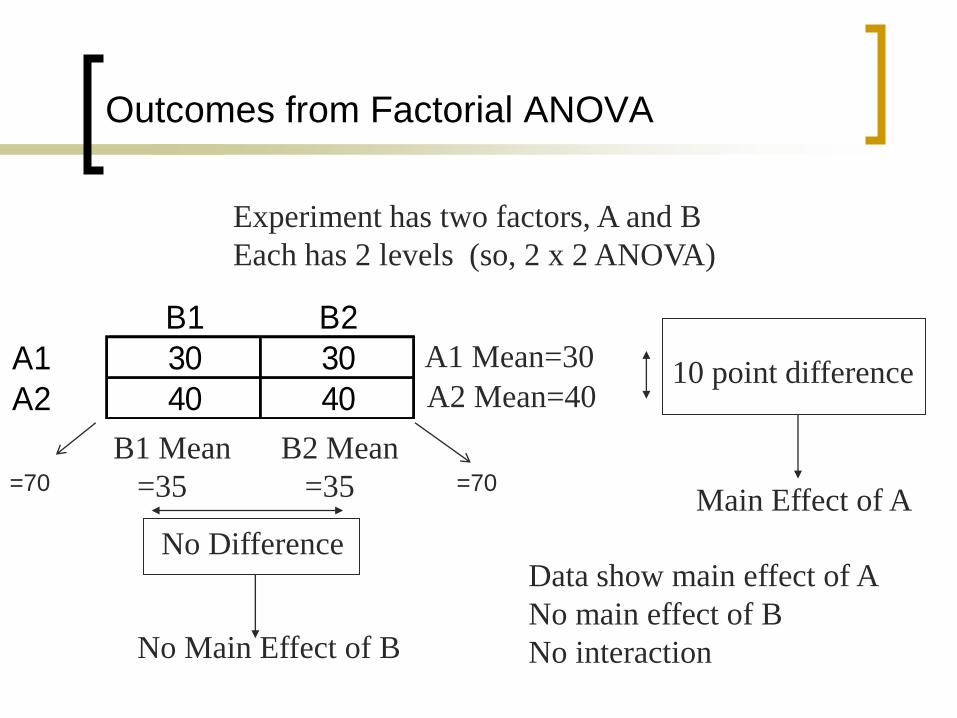
Outcomes from Factorial ANOVA
B1 B2
A1 30 30
A2 40 40
Experiment has two factors, A and B
Each has 2 levels (so, 2 x 2 ANOVA)
A1 Mean=30
A2 Mean=40
B1 Mean
=35
B2 Mean
=35
10 point difference
No Difference
Main Effect of A
No Main Effect of B
Data show main effect of A
No main effect of B
No interaction
=70=70
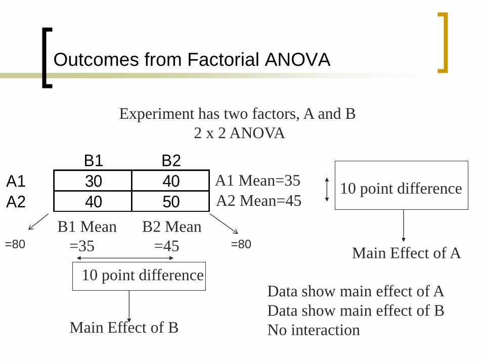
Outcomes from Factorial ANOVA
B1 B2
A1 30 40
A2 40 50
Experiment has two factors, A and B
2 x 2 ANOVA
A1 Mean=35
A2 Mean=45
B1 Mean
=35
B2 Mean
=45
10 point difference
10 point difference
Main Effect of A
Main Effect of B
Data show main effect of A
Data show main effect of B
No interaction
=80=80
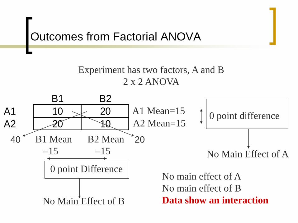
Outcomes from Factorial ANOVA
B1 B2
A1 10 20
A2 20 10
Experiment has two factors, A and B
2 x 2 ANOVA
A1 Mean=15
A2 Mean=15
B1 Mean
=15
B2 Mean
=15
0 point difference
No Main Effect of A
0 point Difference
No Main Effect of B
No main effect of A
No main effect of B
Data show an interaction
2040
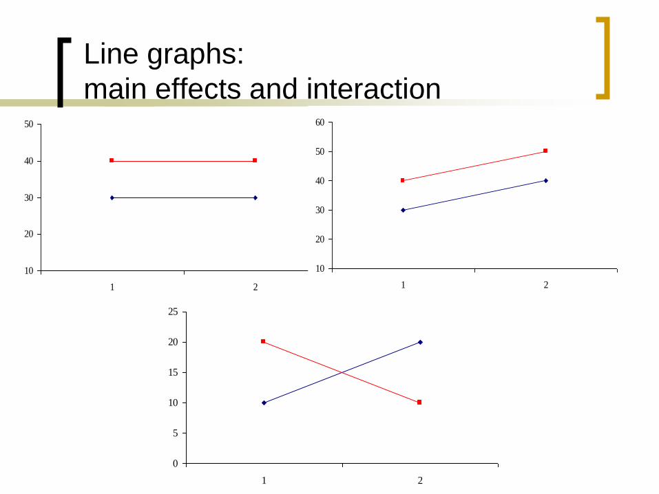
Line graphs:
main effects and interaction
10
20
30
40
50
1 2
10
20
30
40
50
60
1 2
0
5
10
15
20
25
1 2
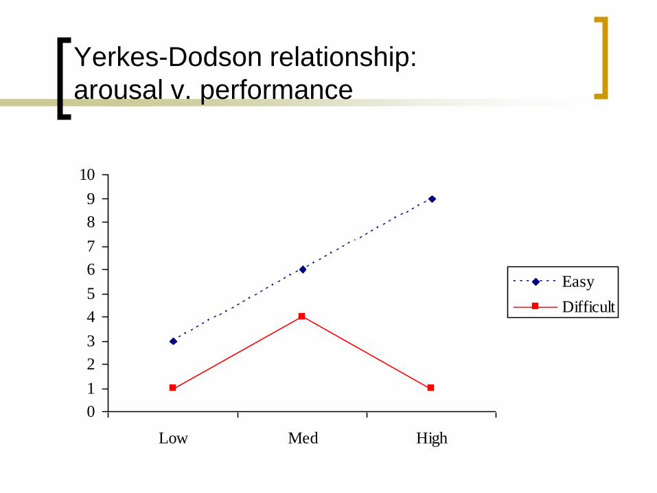
Yerkes-Dodson relationship:
arousal v. performance
0
1
2
3
4
5
6
7
8
9
10
Low Med High
Easy
Difficult
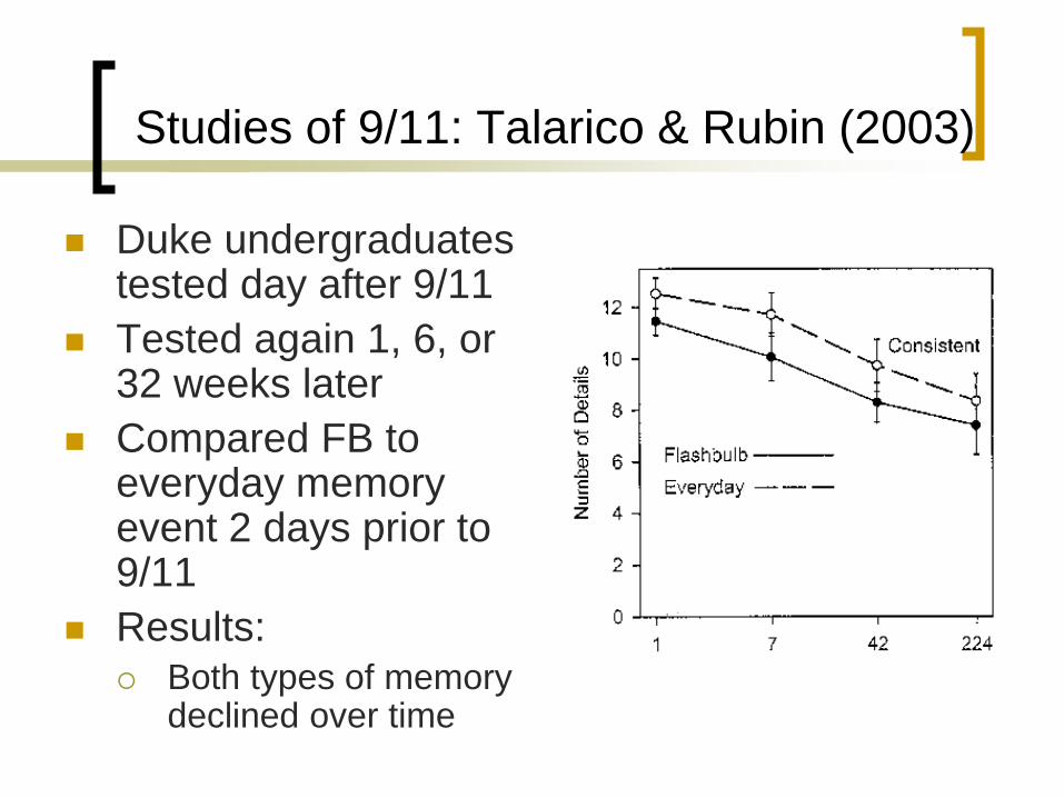
Studies of 9/11: Talarico & Rubin (2003)
Duke undergraduates tested day after 9/11
Tested again 1, 6, or 32 weeks later
Compared FB to everyday memory event 2 days prior to 9/11
Results: Both types of memory
declined over time
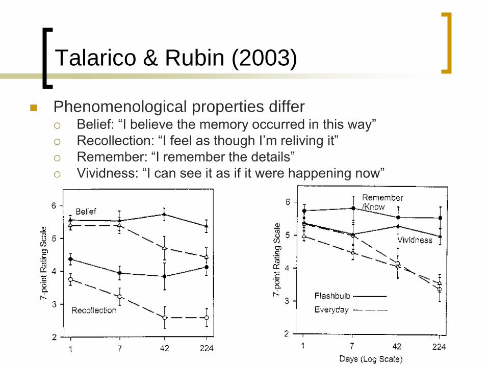
Talarico & Rubin (2003)
Phenomenological properties differ Belief: “I believe the memory occurred in this way”
Recollection: “I feel as though I’m reliving it”
Remember: “I remember the details”
Vividness: “I can see it as if it were happening now”
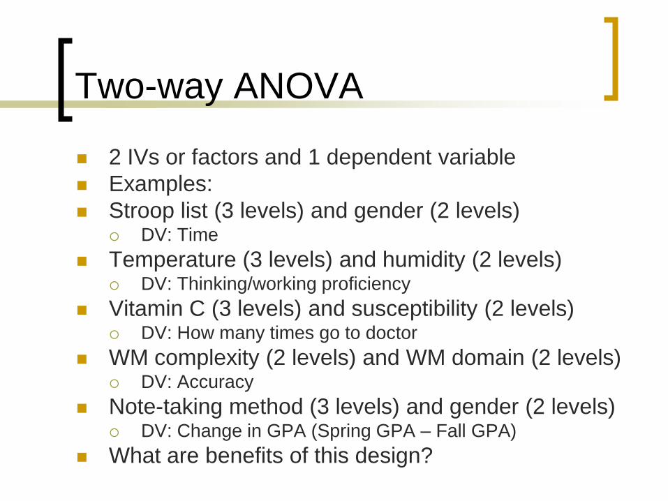
Two-way ANOVA
2 IVs or factors and 1 dependent variable
Examples:
Stroop list (3 levels) and gender (2 levels) DV: Time
Temperature (3 levels) and humidity (2 levels) DV: Thinking/working proficiency
Vitamin C (3 levels) and susceptibility (2 levels) DV: How many times go to doctor
WM complexity (2 levels) and WM domain (2 levels) DV: Accuracy
Note-taking method (3 levels) and gender (2 levels) DV: Change in GPA (Spring GPA – Fall GPA)
What are benefits of this design?
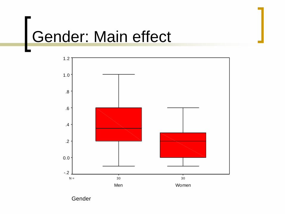
Gender: Main effect
3030N =
Gender
WomenMen
Ch
an
ge
in
GP
A
1.2
1.0
.8
.6
.4
.2
0.0
-.2
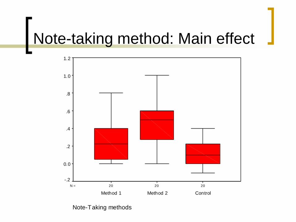
Note-taking method: Main effect
202020N =
Note-Taking methods
ControlMethod 2Method 1
Ch
an
ge
in
GP
A
1.2
1.0
.8
.6
.4
.2
0.0
-.2
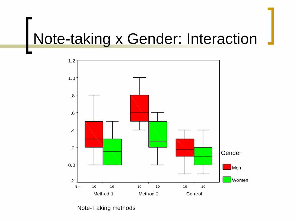
Note-taking x Gender: Interaction
101010 101010N =
Note-Taking methods
ControlMethod 2Method 1
Ch
an
ge
in
GP
A
1.2
1.0
.8
.6
.4
.2
0.0
-.2
Gender
Men
Women
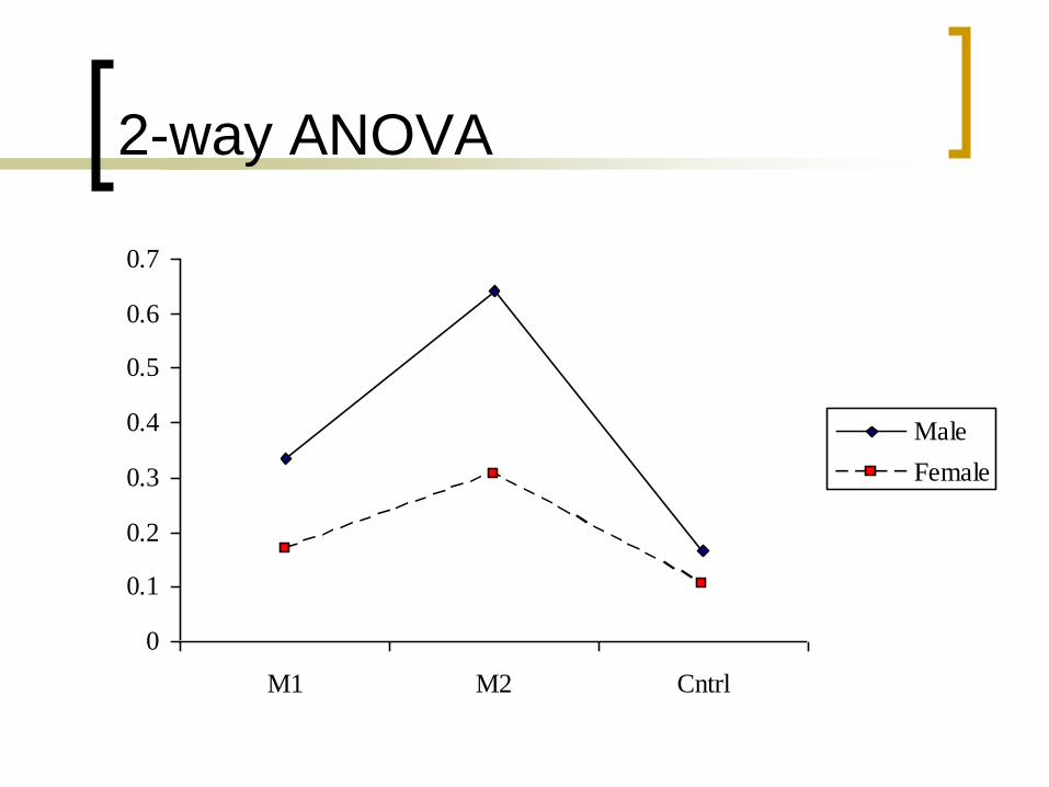
2-way ANOVA
0
0.1
0.2
0.3
0.4
0.5
0.6
0.7
M1 M2 Cntrl
Male
Female
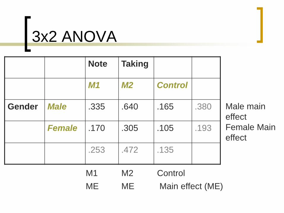
3x2 ANOVA
Note Taking
M1 M2 Control
Gender Male .335 .640 .165 .380
Female .170 .305 .105 .193
.253 .472 .135
Male main
effect
Female Main
effect
M1 M2 Control
ME ME Main effect (ME)
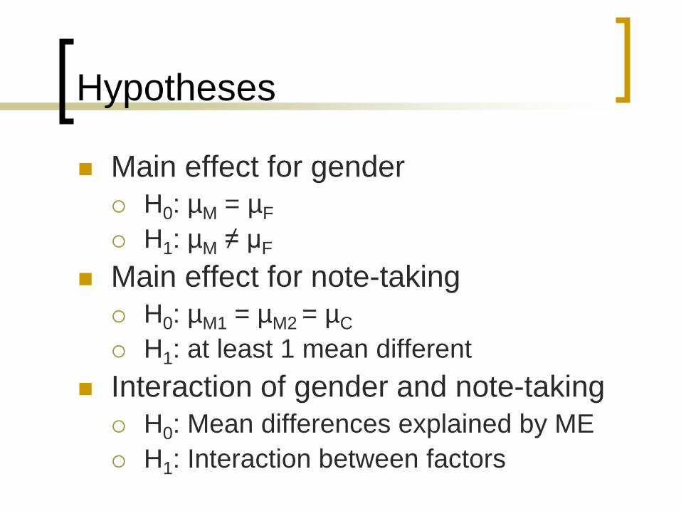
Hypotheses
Main effect for gender
H0: µM = µF
H1: µM ≠ µF
Main effect for note-taking
H0: µM1 = µM2 = µC
H1: at least 1 mean different
Interaction of gender and note-taking
H0: Mean differences explained by ME
H1: Interaction between factors
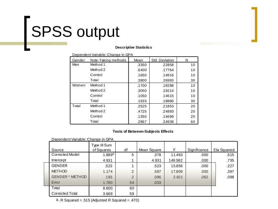
SPSS outputDescriptive Statistics
Dependent Variable: Change in GPA
.3350 .22858 10
.6400 .17764 10
.1650 .14916 10
.3800 .26993 30
.1700 .18288 10
.3050 .19214 10
.1050 .14615 10
.1933 .18880 30
.2525 .21853 20
.4725 .24893 20
.1350 .14699 20
.2867 .24938 60
Note-Taking methods
Method 1
Method 2
Control
Total
Method 1
Method 2
Control
Total
Method 1
Method 2
Control
Total
Gender
Men
Women
Total
Mean Std. Deviation N
Tests of Between-Subjects Effects
Dependent Variable: Change in GPA
1.889a 5 .378 11.463 .000 .515
4.931 1 4.931 149.582 .000 .735
.523 1 .523 15.856 .000 .227
1.174 2 .587 17.809 .000 .397
.193 2 .096 2.921 .062 .098
1.780 54 .033
8.600 60
3.669 59
Source
Corrected Model
Intercept
GENDER
METHOD
GENDER * METHOD
Error
Total
Corrected Total
Type III Sum
of Squares df Mean Square F Significance Eta Squared
R Squared = .515 (Adjusted R Squared = .470)a.
2-way ANOVA
0
0.1
0.2
0.3
0.4
0.5
0.6
0.7
M1 M2 Cntrl
Male
Female
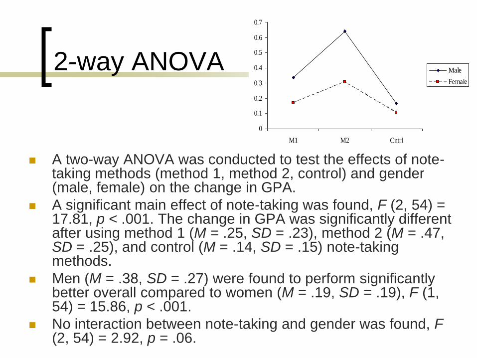
A two-way ANOVA was conducted to test the effects of note-taking methods (method 1, method 2, control) and gender (male, female) on the change in GPA.
A significant main effect of note-taking was found, F (2, 54) = 17.81, p < .001. The change in GPA was significantly different after using method 1 (M = .25, SD = .23), method 2 (M = .47, SD = .25), and control (M = .14, SD = .15) note-taking methods.
Men (M = .38, SD = .27) were found to perform significantly better overall compared to women (M = .19, SD = .19), F (1, 54) = 15.86, p < .001.
No interaction between note-taking and gender was found, F(2, 54) = 2.92, p = .06.
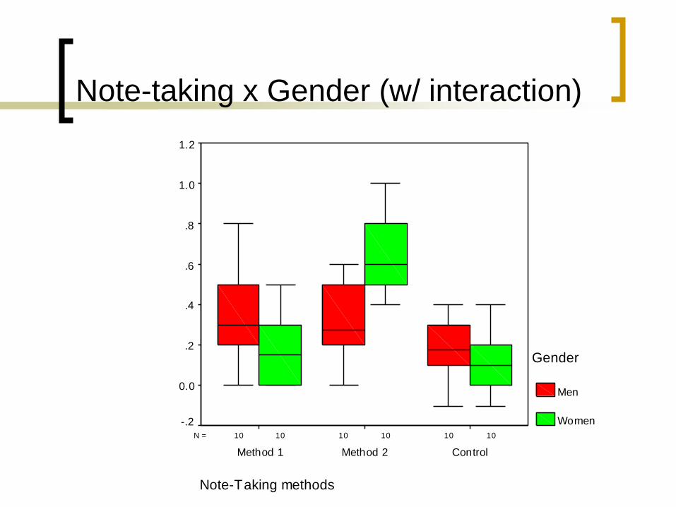
Note-taking x Gender (w/ interaction)
101010 101010N =
Note-Taking methods
ControlMethod 2Method 1
Ch
an
ge
in
GP
A
1.2
1.0
.8
.6
.4
.2
0.0
-.2
Gender
Men
Women
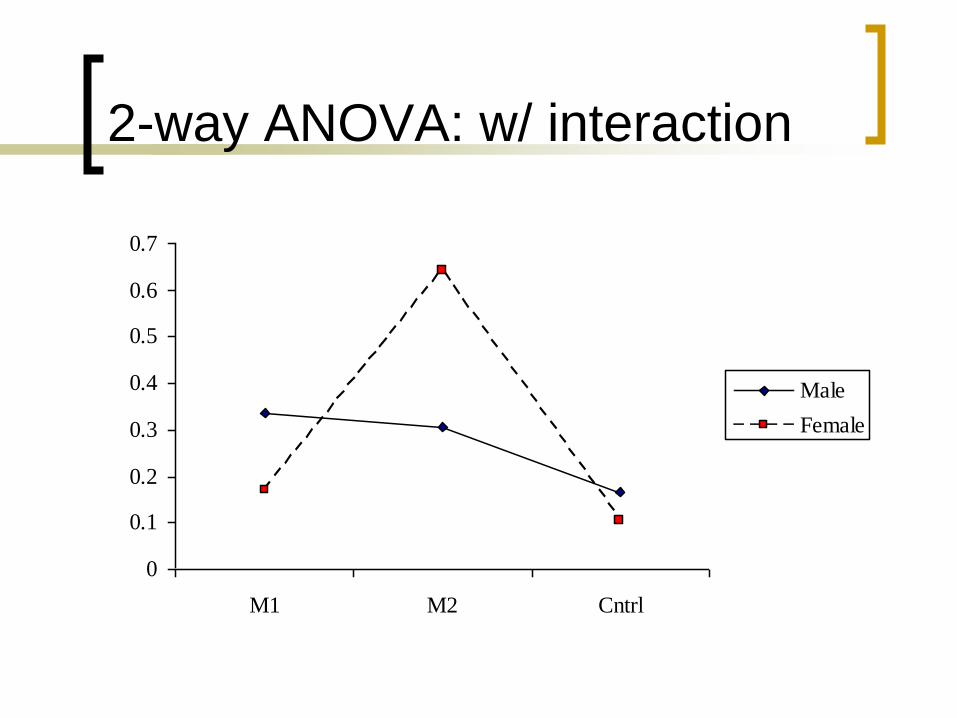
2-way ANOVA: w/ interaction
0
0.1
0.2
0.3
0.4
0.5
0.6
0.7
M1 M2 Cntrl
Male
Female
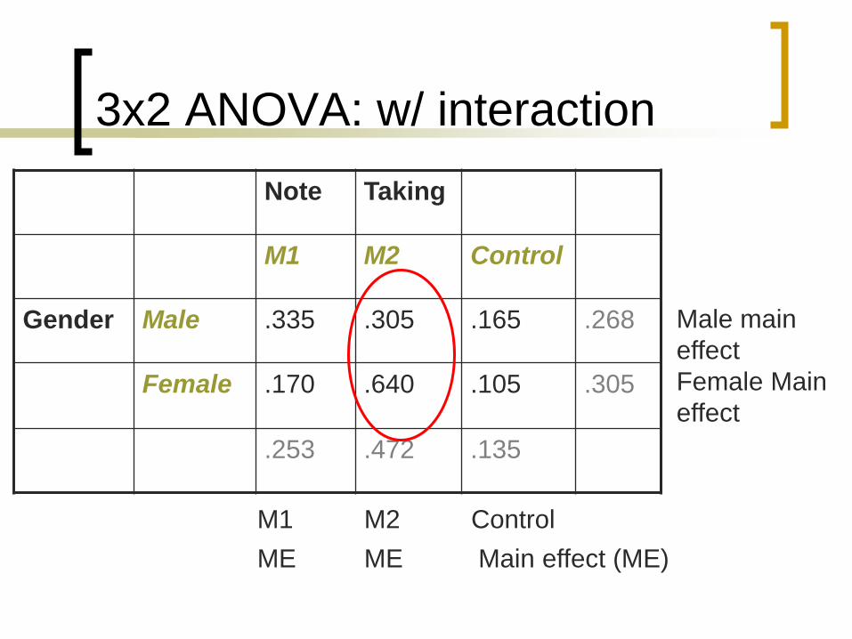
3x2 ANOVA: w/ interaction
Note Taking
M1 M2 Control
Gender Male .335 .305 .165 .268
Female .170 .640 .105 .305
.253 .472 .135
Male main
effect
Female Main
effect
M1 M2 Control
ME ME Main effect (ME)
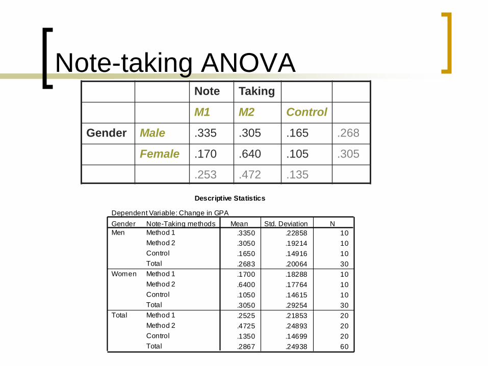
Note-taking ANOVANote Taking
M1 M2 Control
Gender Male .335 .305 .165 .268
Female .170 .640 .105 .305
.253 .472 .135
Descriptive Statistics
Dependent Variable: Change in GPA
.3350 .22858 10
.3050 .19214 10
.1650 .14916 10
.2683 .20064 30
.1700 .18288 10
.6400 .17764 10
.1050 .14615 10
.3050 .29254 30
.2525 .21853 20
.4725 .24893 20
.1350 .14699 20
.2867 .24938 60
Note-Taking methods
Method 1
Method 2
Control
Total
Method 1
Method 2
Control
Total
Method 1
Method 2
Control
Total
Gender
Men
Women
Total
Mean Std. Deviation N
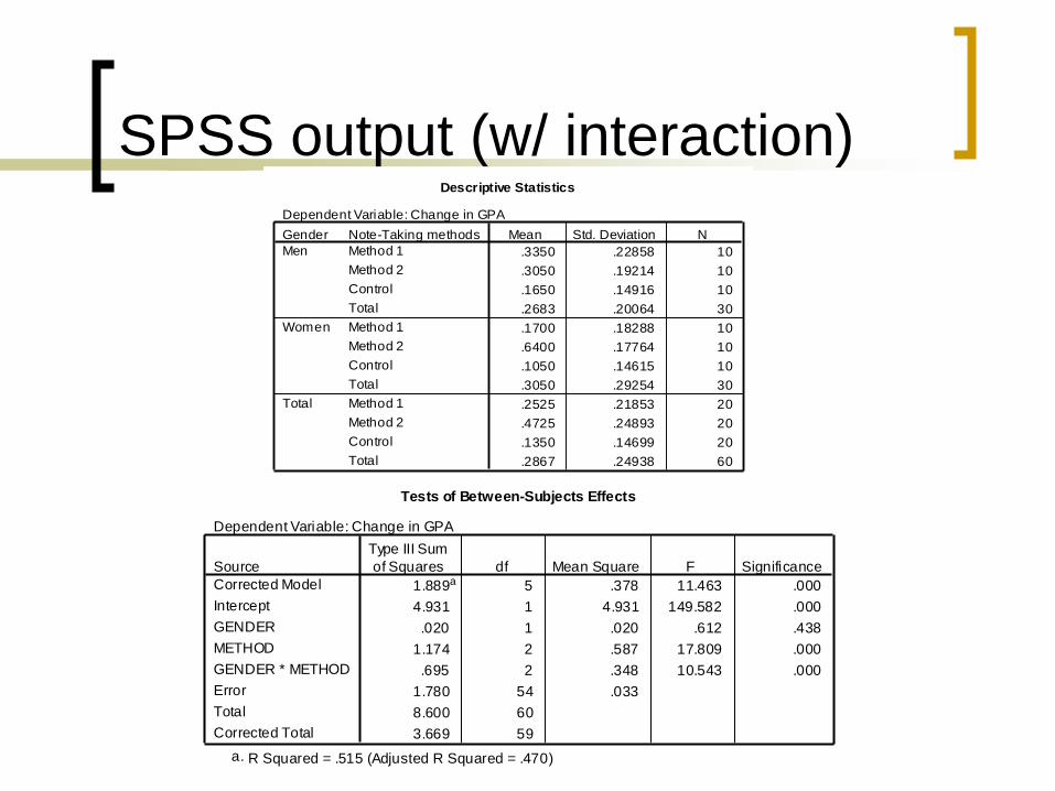
SPSS output (w/ interaction)Descriptive Statistics
Dependent Variable: Change in GPA
.3350 .22858 10
.3050 .19214 10
.1650 .14916 10
.2683 .20064 30
.1700 .18288 10
.6400 .17764 10
.1050 .14615 10
.3050 .29254 30
.2525 .21853 20
.4725 .24893 20
.1350 .14699 20
.2867 .24938 60
Note-Taking methods
Method 1
Method 2
Control
Total
Method 1
Method 2
Control
Total
Method 1
Method 2
Control
Total
Gender
Men
Women
Total
Mean Std. Deviation N
Tests of Between-Subjects Effects
Dependent Variable: Change in GPA
1.889a 5 .378 11.463 .000
4.931 1 4.931 149.582 .000
.020 1 .020 .612 .438
1.174 2 .587 17.809 .000
.695 2 .348 10.543 .000
1.780 54 .033
8.600 60
3.669 59
Source
Corrected Model
Intercept
GENDER
METHOD
GENDER * METHOD
Error
Total
Corrected Total
Type III Sum
of Squares df Mean Square F Significance
R Squared = .515 (Adjusted R Squared = .470)a.
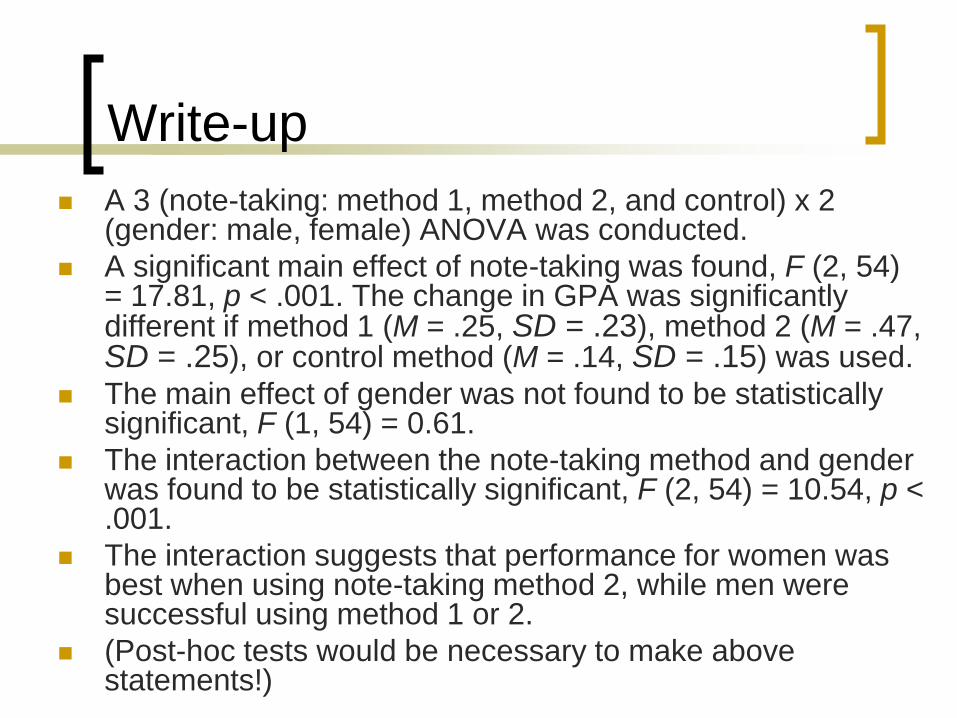
Write-up
A 3 (note-taking: method 1, method 2, and control) x 2 (gender: male, female) ANOVA was conducted.
A significant main effect of note-taking was found, F (2, 54) = 17.81, p < .001. The change in GPA was significantly different if method 1 (M = .25, SD = .23), method 2 (M = .47, SD = .25), or control method (M = .14, SD = .15) was used.
The main effect of gender was not found to be statistically significant, F (1, 54) = 0.61.
The interaction between the note-taking method and gender was found to be statistically significant, F (2, 54) = 10.54, p < .001.
The interaction suggests that performance for women was best when using note-taking method 2, while men were successful using method 1 or 2.
(Post-hoc tests would be necessary to make above statements!)
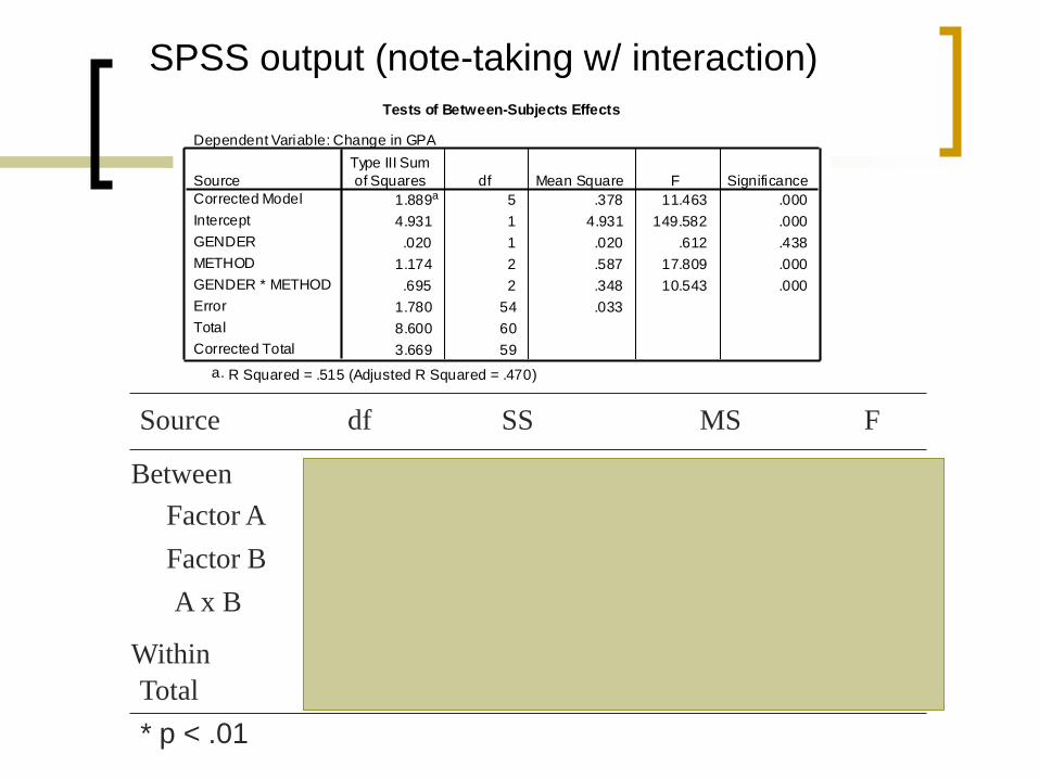
SPSS output (note-taking w/ interaction)
Tests of Between-Subjects Effects
Dependent Variable: Change in GPA
1.889a 5 .378 11.463 .000
4.931 1 4.931 149.582 .000
.020 1 .020 .612 .438
1.174 2 .587 17.809 .000
.695 2 .348 10.543 .000
1.780 54 .033
8.600 60
3.669 59
Source
Corrected Model
Intercept
GENDER
METHOD
GENDER * METHOD
Error
Total
Corrected Total
Type III Sum
of Squares df Mean Square F Significance
R Squared = .515 (Adjusted R Squared = .470)a.
Source df SS MS F
Between
Within
Total
Factor A
Factor B
A x B
5
1
1.889
0.020 0.6120.020
2 1.174 17.809*
2 0.695 10.543*0.348
0.587
54 1.780 0.033
59 3.669
* p < .01
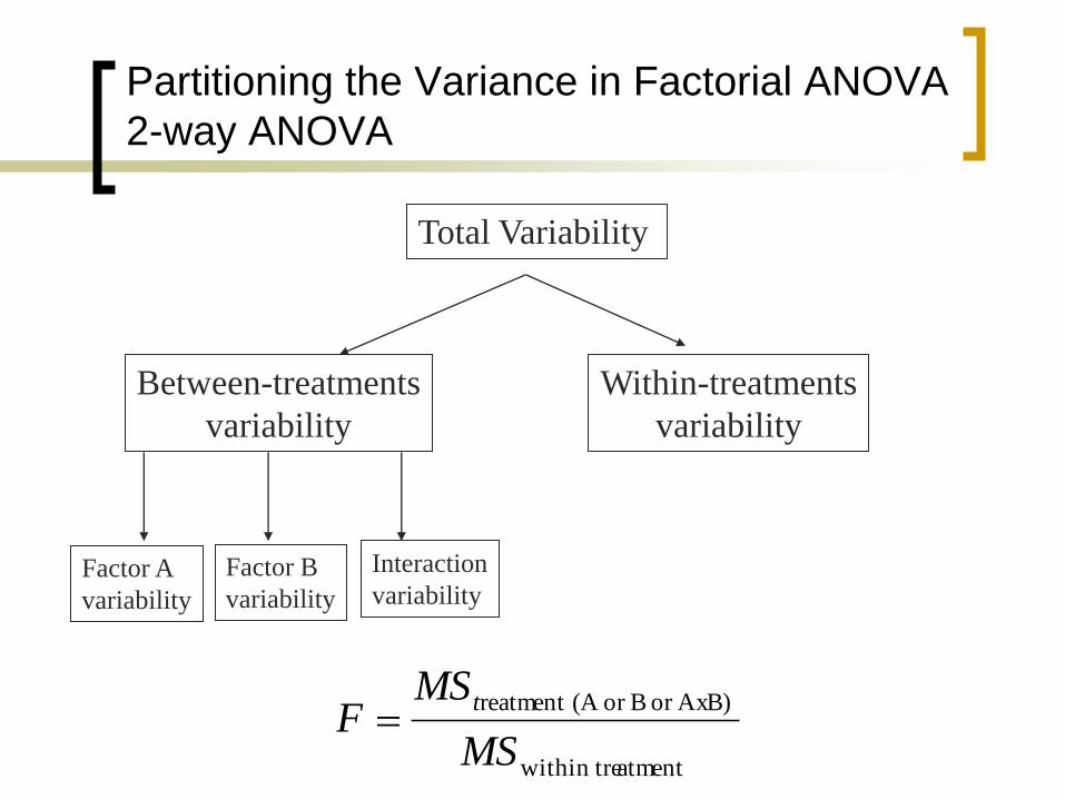
Partitioning the Variance in Factorial ANOVA
2-way ANOVA
Total Variability
Between-treatments
variability
Within-treatments
variability
Factor A
variability
Factor B
variability
Interaction
variability
atmentwithin tre
AxB)or Bor (A reatment
MS
MSF
t
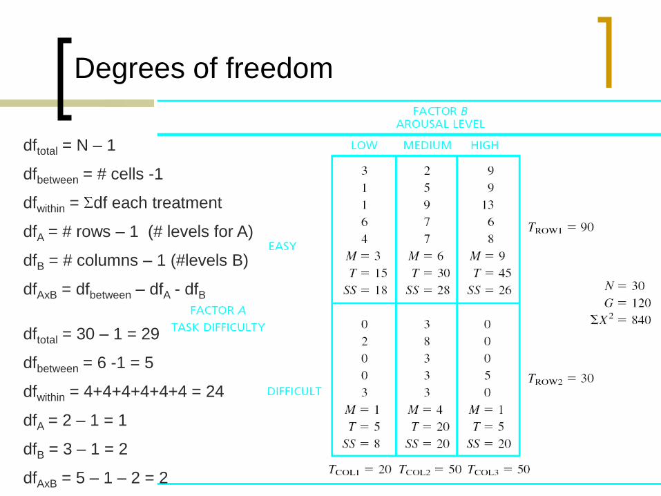
Degrees of freedom
dftotal = N – 1
dfbetween = # cells -1
dfwithin = df each treatment
dfA = # rows – 1 (# levels for A)
dfB = # columns – 1 (#levels B)
dfAxB = dfbetween – dfA - dfB
dftotal = 30 – 1 = 29
dfbetween = 6 -1 = 5
dfwithin = 4+4+4+4+4+4 = 24
dfA = 2 – 1 = 1
dfB = 3 – 1 = 2
dfAxB = 5 – 1 – 2 = 2
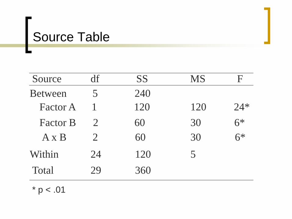
Source Table
Source df SS MS F
Between
Within
Total
Factor A
Factor B
A x B
5
1
240
120 120 24*
2 60 30
2 60 30 6*
6*
24 120 5
29 360
* p < .01