Type-II Generalized Family-Wise Error RateFormulas with Application to Sample Size

Determination

Benoit Liquet1,2, Pierre Lafaye de Micheaux3 and Jeremie Riou4

1 University de Pau et Pays de l’Adour, LMAP.2 ARC Centre of Excellence for Mathematical and Statistical Frontiers

Queensland University of Technology (QUT)

3 CREST-ENSAI (France)

4 Universite d’Angers (France)

Contents

1. Framework: Multiple testing in clinical trial

2. At least one win

3. At lest r wins

4. R code: rPowerSampleSize

5. Concluding remarks

Clinical Context

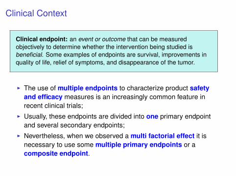
Clinical endpoint: an event or outcome that can be measuredobjectively to determine whether the intervention being studied isbeneficial. Some examples of endpoints are survival, improvements inquality of life, relief of symptoms, and disappearance of the tumor.

I The use of multiple endpoints to characterize product safetyand efficacy measures is an increasingly common feature inrecent clinical trials;

I Usually, these endpoints are divided into one primary endpointand several secondary endpoints;

I Nevertheless, when we observed a multi factorial effect it isnecessary to use some multiple primary endpoints or acomposite endpoint.

Clinical Context

Clinical endpoint: an event or outcome that can be measuredobjectively to determine whether the intervention being studied isbeneficial. Some examples of endpoints are survival, improvements inquality of life, relief of symptoms, and disappearance of the tumor.

I The use of multiple endpoints to characterize product safetyand efficacy measures is an increasingly common feature inrecent clinical trials;

I Usually, these endpoints are divided into one primary endpointand several secondary endpoints;

I Nevertheless, when we observed a multi factorial effect it isnecessary to use some multiple primary endpoints or acomposite endpoint.

Industrial Statistical Challenge in Nutrition

Effects of dairy products are often Multifactorial, Smaller thanpharmaceutical products, with an Higher Variability

Industrial statistical challenge

1. Sample Size Determination in the context of MultiplePrimary Endpoints;

2. Data Analysis in the context of Multiple Primary Endpoints.

Multiple Primary endpoints

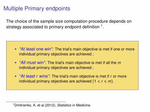
The choice of the sample size computation procedure depends onstrategy associated to primary endpoint definition 1.

I “At least one win”: The trial’s main objective is met if one or moreindividual primary objectives are achieved ;

I “All must win”: The trial’s main objective is met if all the mindividual primary objectives are achieved ;

I “At least r wins”: The trial’s main objective is met if r or moreindividual primary objectives are achieved (1 6 r 6 m).

1Dmitrienko, A. et al.(2012), Statistics in Medicine.

Today Aims

1. Brief description on Sample Size Computation and DataAnalysis in the context of “At least one win” primarycontinuous endpoints;Lafaye de Micheaux P., Liquet B., Marques S. and Riou J., Power and sample size determination in clinical trials

with multiple primary continuous correlated end points. Journal of Biopharmaceutical Statistics 24:2, 378-97,

(2014).

2. More Details on Sample Size Computation Methodology inthe context of “‘At least r wins” primary endpoints.Delorme P., Lafaye de Micheaux P., Liquet B. and Riou J., Type-II Generalized Family-Wise Error Rate Formulas

with Application to Sample Size Determination. Statistics in Medicine (2016) In press.

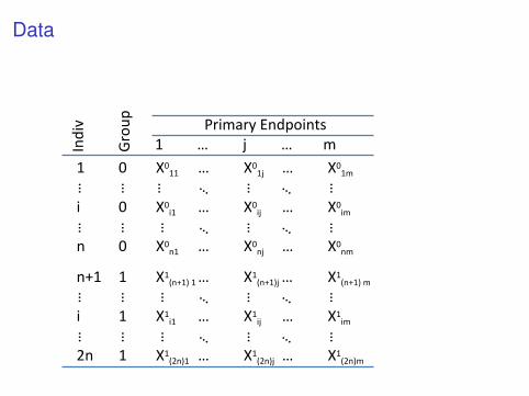
Data

1 0

i 0

n 0

1 … j … m

Primary Endpoints

n+1 1

i 1

2n 1

……

……

……

……

Gro

up

Ind

iv

X011 … X0

1j … X01m

X0i1 … X0

ij … X0im

X0n1 … X0

nj … X0nm

X1(n+1) 1 … X1

(n+1)j … X1(n+1) m

X1i1 … X1

ij … X1im

X1(2n)1 … X1

(2n)j … X1(2n)m

……

……

……

……

……

……

…

…

…

…

… …

…

…

Sample size for one endpoint: single hypothesis testingTrue state of NatureH0 is true H1 is true

DecisionWe decide H1 Type I error No errorWe decide H0 No error Type II error

The Type I error is when one decides H1 while it is H0 that is true.The Type II error is when one decides H0 while it is H1 that is true.

power function = P [not decide H0 when H1 is true]

≡ 1 − β.

Generally easy to determine the necessary sample size n to usein order to control (with some given thresholds) both the maximalType I error rate (under H0) and a Type II error rate (under H1).

Sample size for one endpoint: single hypothesis testingTrue state of NatureH0 is true H1 is true

DecisionWe decide H1 Type I error No errorWe decide H0 No error Type II error

The Type I error is when one decides H1 while it is H0 that is true.The Type II error is when one decides H0 while it is H1 that is true.

power function = P [not decide H0 when H1 is true]

≡ 1 − β.

Generally easy to determine the necessary sample size n to usein order to control (with some given thresholds) both the maximalType I error rate (under H0) and a Type II error rate (under H1).

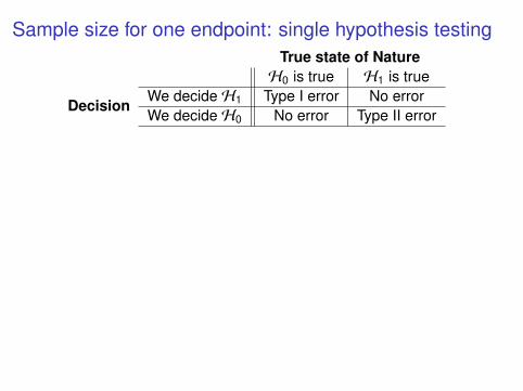
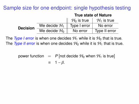
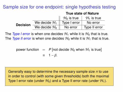
Sample size for one endpoint: single hypothesis testingTrue state of NatureH0 is true H1 is true

DecisionWe decide H1 Type I error No errorWe decide H0 No error Type II error

The Type I error is when one decides H1 while it is H0 that is true.The Type II error is when one decides H0 while it is H1 that is true.

power function = P [not decide H0 when H1 is true]

≡ 1 − β.

Generally easy to determine the necessary sample size n to usein order to control (with some given thresholds) both the maximalType I error rate (under H0) and a Type II error rate (under H1).

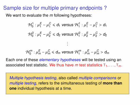
Sample size for multiple primary endpoints ?We want to evaluate the m following hypotheses:

H10 : µE

1 − µC1 6 d1 versus H1

1 : µE1 − µ

C1 > d1

H20 : µE

1 − µC2 6 d2 versus H2

1 : µE2 − µ

C2 > d2

...

Hm0 : µE

m − µCm 6 dm versus Hm

1 : µEm − µ

Cm > dm

Each one of these elementary hypotheses will be tested using anassociated test statistic. We thus have m test statistics T1, . . . , Tm.

Multiple hypothesis testing, also called multiple comparisons ormultiple testing, refers to the simultaneous testing of more thanone individual hypothesis at a time.

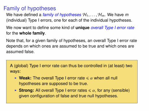
Family of hypothesesWe have defined a family of hypotheses H1, . . . ,Hm. We have m(individual) Type I errors, one for each of the individual hypotheses.

We now want to define some kind of unique overall Type I error ratefor the whole family.

Note that, for a given family of hypotheses, an overall Type I error ratedepends on which ones are assumed to be true and which ones areassumed false.

A (global) Type I error rate can thus be controlled in (at least) twoways:I Weak: The overall Type I error rate 6 α when all null

hypotheses are supposed to be true.I Strong: All overall Type I error rates 6 α, for any (sensible)

given configuration of false and true null hypotheses.

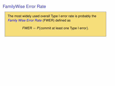
FamilyWise Error Rate

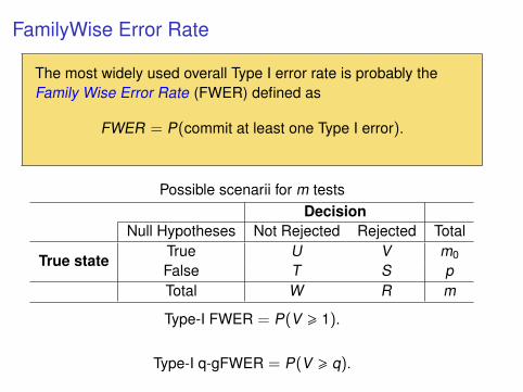
The most widely used overall Type I error rate is probably theFamily Wise Error Rate (FWER) defined as

FWER = P(commit at least one Type I error).

Possible scenarii for m testsDecision

Null Hypotheses Not Rejected Rejected Total

True stateTrue U V m0

False T S pTotal W R m

Type-I FWER = P(V > 1).

Type-I q-gFWER = P(V > q).

FamilyWise Error Rate

The most widely used overall Type I error rate is probably theFamily Wise Error Rate (FWER) defined as

FWER = P(commit at least one Type I error).

Possible scenarii for m testsDecision

Null Hypotheses Not Rejected Rejected Total

True stateTrue U V m0

False T S pTotal W R m

Type-I FWER = P(V > 1).

Type-I q-gFWER = P(V > q).

Power control

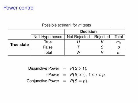
Possible scenarii for m tests

DecisionNull Hypotheses Not Rejected Rejected Total

True stateTrue U V m0

False T S pTotal W R m

Disjunctive Power = P(S > 1),

r-Power = P(S > r), 1 6 r 6 p,

Conjunctive Power = P(S = p).

At least one win: Individual testing approach

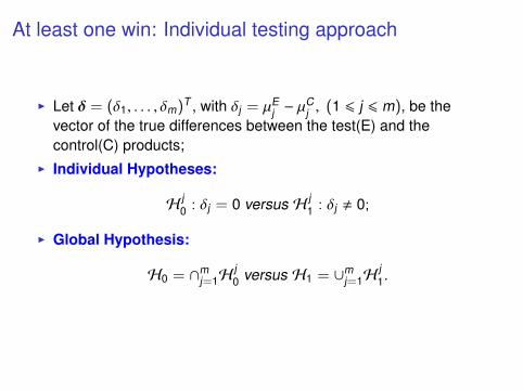
I Let δ = (δ1, . . . , δm)T , with δj = µEj − µ

Cj , (1 6 j 6 m), be the

vector of the true differences between the test(E) and thecontrol(C) products;

I Individual Hypotheses:

Hj0 : δj = 0 versus H j

1 : δj , 0;

I Global Hypothesis:

H0 = ∩mj=1H

j0 versus H1 = ∪m

j=1Hj1.

Statistics

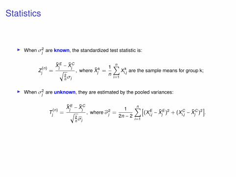
I When σ2j are known, the standardized test statistic is:

Z(n)j =

XEj − XC

j√2nσj

, where Xkj =

1n

n∑i=1

Xki,j are the sample means for group k;

I When σ2j are unknown, they are estimated by the pooled variances:

T (n)j =

XEj − XC

j√2n σj

, where σ2j =

12n − 2

n∑i=1

[(XE

i,j − XEj )2 + (XC

i,j − XCj )2

].

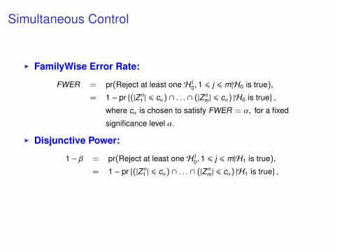
Simultaneous Control

I FamilyWise Error Rate:

FWER = pr(Reject at least one H j0, 1 6 j 6 m|H0 is true),

= 1 − pr{(|Zn

1 | 6 cα) ∩ . . . ∩ (|Znm | 6 cα) |H0 is true

},

where cα is chosen to satisfy FWER = α, for a fixed

significance level α.

I Disjunctive Power:

1 − β = pr(Reject at least one H j0, 1 6 j 6 m|H1 is true),

= 1 − pr{(|Zn

1 | 6 cα) ∩ . . . ∩ (|Znm | 6 cα) |H1 is true

},

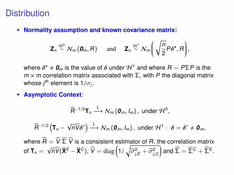
Distribution

I Normality assumption and known covariance matrix:

ZnH0

∼ Nm (0m,R) and ZnH1

∼ Nm

√n2

Pδ∗,R ,

where δ∗ , 0m is the value of δ under H1 and where R = PΣP is them ×m correlation matrix associated with Σ, with P the diagonal matrixwhose jth element is 1/σj .

I Asymptotic Context:

R−1/2TnL−→ Nm (0m, Im) , under H0,

R−1/2(Tn −

√nVδ∗

) L−→ Nm (0m, Im) , under H1 : δ = δ∗ , 0m,

where R = V Σ V is a consistent estimator of R, the correlation matrixof Tn =

√nV(XE − XC), V = diag

(1/

√σ2

j,E + σ2j,C

)and Σ = ΣC + ΣE .

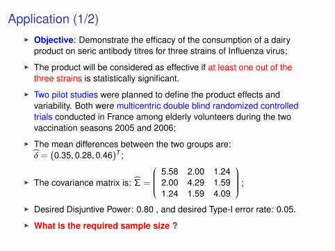
Application (1/2)I Objective: Demonstrate the efficacy of the consumption of a dairy

product on seric antibody titres for three strains of Influenza virus;

I The product will be considered as effective if at least one out of thethree strains is statistically significant.

I Two pilot studies were planned to define the product effects andvariability. Both were multicentric double blind randomized controlledtrials conducted in France among elderly volunteers during the twovaccination seasons 2005 and 2006;

I The mean differences between the two groups are:δ = (0.35, 0.28, 0.46)T ;

I The covariance matrix is: Σ =

5.58 2.00 1.242.00 4.29 1.591.24 1.59 4.09

;

I Desired Disjuntive Power: 0.80 , and desired Type-I error rate: 0.05.

I What is the required sample size ?

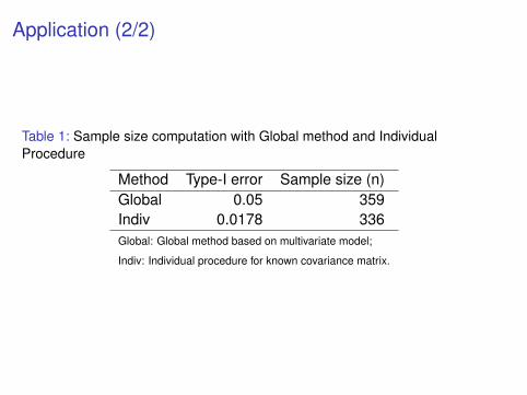
Application (2/2)

Table 1: Sample size computation with Global method and IndividualProcedure

Method Type-I error Sample size (n)Global 0.05 359Indiv 0.0178 336Global: Global method based on multivariate model;

Indiv: Individual procedure for known covariance matrix.

At least r wins

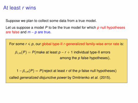
Suppose we plan to collect some data from a true model.

Let us suppose a model P to be the true model for which p null hypothesesare false and m − p are true.

For some r 6 p, our global type-II r-generalized family-wise error rate is:

βr ,m(P) = P(make at least p − r + 1 individual type-II errors

among the p false hypotheses),

1 − βr ,m(P) = P(reject at least r of the p false null hypotheses)

called generalized disjunctive power by Dmitrienko et al. (2015).

Motivation: Clinical trial in vaccinationANRS 114 Pneumovac trial: measure the effect of two vaccinestrategies against Streptococcus pneumoniae in adults infected bythe HIV, which are more susceptible to infections caused by thisbacterial pathogen.

Seven (m = 7) clinical endpoints: log-transformed (towardsGaussianity) measurements of serotype-specific antibody titerconcentrations (continuous measurements in µg/ml).

Note: serotype refers to distinct variations within a species of bacteriaor viruses or among immune cells of different individuals.

Pedrono et al. (2009) suggest that one vaccine strategy might beconsidered as superior to the other when at least 3, 5 or 7serotypes are found significant.

Aim: compute the sample sizes necessary for a weak control ofthe r-power for r = 3, 5, 7 for different multiple procedure.

Motivation: Clinical trial in vaccinationANRS 114 Pneumovac trial: measure the effect of two vaccinestrategies against Streptococcus pneumoniae in adults infected bythe HIV, which are more susceptible to infections caused by thisbacterial pathogen.

Seven (m = 7) clinical endpoints: log-transformed (towardsGaussianity) measurements of serotype-specific antibody titerconcentrations (continuous measurements in µg/ml).

Note: serotype refers to distinct variations within a species of bacteriaor viruses or among immune cells of different individuals.

Pedrono et al. (2009) suggest that one vaccine strategy might beconsidered as superior to the other when at least 3, 5 or 7serotypes are found significant.

Aim: compute the sample sizes necessary for a weak control ofthe r-power for r = 3, 5, 7 for different multiple procedure.

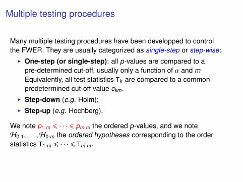
Multiple testing procedures

Many multiple testing procedures have been developped to controlthe FWER. They are usually categorized as single-step or step-wise:I One-step (or single-step): all p-values are compared to a

pre-determined cut-off, usually only a function of α and mEquivalently, all test statistics Tk are compared to a commonpredetermined cut-off value ckm.

I Step-down (e.g. Holm);I Step-up (e.g. Hochberg).

We note p1:m 6 · · · 6 pm:m the ordered p-values, and we noteH0:1, . . . ,H0:m the ordered hypotheses corresponding to the orderstatistics T1:m 6 · · · 6 Tm:m.

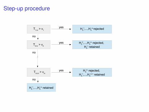
Step-up procedure

T1:m

> v1

H0

1,...,H0

m rejected

T2:m

> v2

H02,...,H

0m rejected,

H0

1 retained

Tm:m

> vm

H0

m rejected, H

01,...,H

0m-1 retained

H0

1,...,H0

m retained

yes

yes

yes

no

no

no

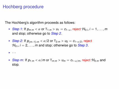
Hochberg procedure

The Hochberg’s algorithm proceeds as follows:

I Step 1: If pm:m < α or T1:m > u1 = c1−α, reject H0:i , i = 1, . . . ,mand stop; otherwise go to Step 2.

I Step 2: If p(m−1):m < α/2 or T2:m > u2 = c1−α/2, rejectH0:i , i = 2, . . . ,m and stop; otherwise go to Step 3.

I · · ·

I Step m: If p1:m < α/m or Tm:m > um = c1−α/m, reject H0:m andstop.

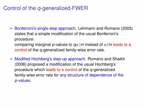
Control of the q-generalized-FWER

I Bonferroni’s single-step approach. Lehmann and Romano (2005)states that a simple modification of the usual Bonferroni’sprocedure:comparing marginal p-values to qα/m instead of α/m leads to acontrol of the q-generalized family-wise error rate.

I Modified Hochberg’s step-up approach. Romano and Shaikh(2006) proposed a modification of the usual Hochberg’sprocedure which leads to a control of the q-generalizedfamily-wise error rate for any structure of dependence of thep-values.

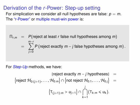
Derivation of the r-Power: Step-up settingFor simplication we consider all null hypotheses are false: p = m.The “r-Power” or multiple must-win power is:

Πr ,m = P(reject at least r false null hypotheses among m)

=m−r∑j=0

P (reject exactly m − j false hypotheses among m) .

For Step-Up methods, we have:

{reject exactly m − j hypotheses} ={reject H0:(j+1), . . . ,H0:m

}∩

{not reject H0:1, . . . ,H0:j

}={

T(j+1):m > uj+1

}∩

j⋂k=1

(Tk :m 6 uk ).

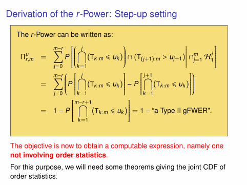
Derivation of the r-Power: Step-up setting

The r-Power can be written as:

Πur ,m =

m−r∑j=0

P

j⋂

k=1

(Tk :m 6 uk )

∩ (T(j+1):m > uj+1)

∣∣∣∣∣∣∣ ∩mj=1 H

j1

=

m−r∑j=0

P j⋂k=1

(Tk :m 6 uk )

− P

j+1⋂k=1

(Tk :m 6 uk )

= 1 − P

m−r+1⋂k=1

(Tk :m 6 uk )

= 1 − “a Type II gFWER”.

The objective is now to obtain a computable expression, namely onenot involving order statistics.

For this purpose, we will need some theorems giving the joint CDF oforder statistics.

Theorem of Maurer and Margolin (1976):

Let ` = (`1, . . . , `q) such that 1 6 `1 6 . . . 6 `q 6 m andu`1 6 . . . 6 u`q . We obtain the joint distribution of orderstatistics:

P

q⋂h=1

(T`h :m 6 u`h )

= (−1)`+

a∗∑a=`

(−1)a+Pa

q∏i=1

((∆ai) − 1

ai − `i

)

with `+ =∑q

h=1 `h , ∆ai = ai − ai−1 and

Pa =∑

j∈J (a,m)P[⋂q−1

i=0

(⋂ai+1k=ai+1 Tjk 6 u`i+1

)].

⇒We can now replace ordered statistics with unordered ones!

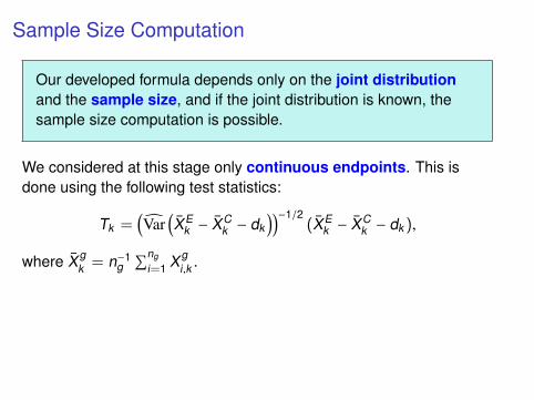
Sample Size Computation

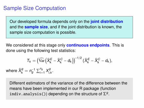
Our developed formula depends only on the joint distributionand the sample size, and if the joint distribution is known, thesample size computation is possible.

We considered at this stage only continuous endpoints. This isdone using the following test statistics:

Tk =(Var

(XE

k − XCk − dk

))−1/2(XE

k − XCk − dk ),

where Xgk = n−1

g∑ng

i=1 Xgi,k .

Different estimators of the variance of the difference between themeans have been implemented in our R package (functionindiv.analysis()) depending on the structure of Σg.

Sample Size Computation

Our developed formula depends only on the joint distributionand the sample size, and if the joint distribution is known, thesample size computation is possible.

We considered at this stage only continuous endpoints. This isdone using the following test statistics:

Tk =(Var

(XE

k − XCk − dk

))−1/2(XE

k − XCk − dk ),

where Xgk = n−1

g∑ng

i=1 Xgi,k .

Different estimators of the variance of the difference between themeans have been implemented in our R package (functionindiv.analysis()) depending on the structure of Σg.

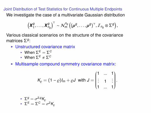
Joint Distribution of Test Statistics for Continuous Multiple EndpointsWe investigate the case of a multivariate Gaussian distribution(

Xg1, . . . ,X

gng

)>∼ N

ngm

((µg, . . . ,µg)>,Ing ⊗ Σg

),

Various classical scenarios on the structure of the covariancematrices Σg:I Unstructured covariance matrix

I When ΣE = ΣC

I When ΣE , ΣC

I Multisample compound symmetry covariance matrix:

K% = (1 − %)Im + %J with J =

1 ... 1... 1

...

1 ... 1

.I Σg = σ2,gK%

I ΣE = ΣC = σ2K%

Joint Distribution of Test Statistics for Continuous Multiple Endpoints

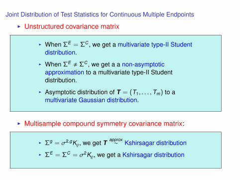
I Unstructured covariance matrix

I When ΣE = ΣC , we get a multivariate type-II Studentdistribution.

I When ΣE , ΣC , we get a a non-asymptoticapproximation to a multivariate type-II Studentdistribution.

I Asymptotic distribution of T = (T1, . . . ,Tm) to amultivariate Gaussian distribution.

I Multisample compound symmetry covariance matrix:

I Σg = σ2,gK%, we get T approx∼ Kshirsagar distribution

I ΣE = ΣC = σ2K%, we get a Kshirsagar distribution

Joint Distribution of Test Statistics for Continuous Multiple Endpoints

I Unstructured covariance matrix

I When ΣE = ΣC , we get a multivariate type-II Studentdistribution.

I When ΣE , ΣC , we get a a non-asymptoticapproximation to a multivariate type-II Studentdistribution.

I Asymptotic distribution of T = (T1, . . . ,Tm) to amultivariate Gaussian distribution.

I Multisample compound symmetry covariance matrix:

I Σg = σ2,gK%, we get T approx∼ Kshirsagar distribution

I ΣE = ΣC = σ2K%, we get a Kshirsagar distribution

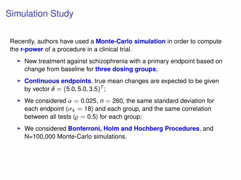
Simulation Study

Recently, authors have used a Monte-Carlo simulation in order to computethe r-power of a procedure in a clinical trial.

I New treatment against schizophrenia with a primary endpoint based onchange from baseline for three dosing groups;

I Continuous endpoints, true mean changes are expected to be givenby vector δ = (5.0, 5.0, 3.5)T ;

I We considered α = 0.025, n = 260, the same standard deviation foreach endpoint (σk = 18) and each group, and the same correlationbetween all tests (% = 0.5) for each group;

I We considered Bonferroni, Holm and Hochberg Procedures, andN=100,000 Monte-Carlo simulations.

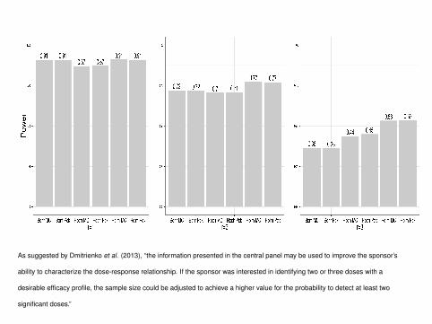
As suggested by Dmitrienko et al. (2013), “the information presented in the central panel may be used to improve the sponsor’s

ability to characterize the dose-response relationship. If the sponsor was interested in identifying two or three doses with a

desirable efficacy profile, the sample size could be adjusted to achieve a higher value for the probability to detect at least two

significant doses.”

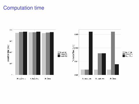
Computation time

Application to he Pneumovac trialI Endpoints used for the evaluation of immunogenicity in the

Vaccine trials are means of antibody concentrations for eachserotype;

I Data comes from ANRS 114 Pneumovac Trial, where themultivalent vaccine yields a response on 7 serotypes;

I Effect size and correlation were taken in Pedrono et al. (2009).I We assume a common unstructured covariance matrix for both

vaccinal strategies

Normal Kshirsagarr = 3 r = 5 r = 7 r = 3 r = 5 r = 7

Bonferroni 21 50 201 22 52 202Hochberg (modified) 23 48 147 24 49 148Holm 20 41 116 21 42 116

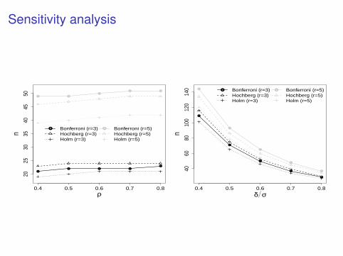
Sensitivity analysis

●

● ● ●

●

0.4 0.5 0.6 0.7 0.8

2025

3035

4045

50

ρ

n

● ●

●

● ●

● ●Bonferroni (r=3)Hochberg (r=3)Holm (r=3)

Bonferroni (r=5)Hochberg (r=5)Holm (r=5)

●

●

●

●

●

0.4 0.5 0.6 0.7 0.840

6080

100

120

140

δ σ

n

●

●

●

●

●

● ●Bonferroni (r=3)Hochberg (r=3)Holm (r=3)

Bonferroni (r=5)Hochberg (r=5)Holm (r=5)

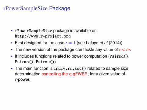
rPowerSampleSize Package

I rPowerSampleSize package is available onhttp://www.r-project.org

I First designed for the case r = 1 (see Lafaye et al (2014))I The new version of the package can tackle any value of r 6 m.I It includes functions related to power computation (Psirmd(),Psirms(), Psirmu())

I The main function is indiv.rm.ssc() related to sample sizedetermination controlling the q-gFWER, for a given value ofr-power.

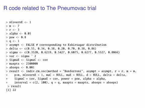
R code related to The Pneumovac trial

> nCovernE <- 1

> m <- 7

> r <- 3

> alpha <- 0.05

> pow <- 0.8

> q <- 1

> asympt <- FALSE # corresponding to Kshirsagar distribution

> delta <- c(0.55, 0.34, 0.38, 0.20, 0.70, 0.38, 0.86)

> sigma <- c(0.3520, 0.6219, 0.5427, 0.6075, 0.6277, 0.5527, 0.8066)

> var <- sigma ˆ 2

> SigmaE <- SigmaC <- cov

> maxpts <- 2500000

> abseps <- 0.001

> result <- indiv.rm.ssc(method = "Bonferroni", asympt = asympt, r = r, m = m,

+ p=m, nCovernE = 1, muC = NULL, muE = NULL, d = NULL, delta = delta,

+ SigmaC = cov, SigmaE = cov, power = pow, alpha = alpha,

+ interval = c(2, 100), q = q, maxpts = maxpts, abseps = abseps)

> result

[1] 22

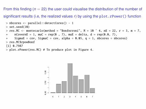
From this finding (n = 22) the user could visualise the distribution of the number of

significant results (i.e, the realized values r) by using the plot.rPower() function

> nbcores <- parallel::detectCores() - 1

> set.seed(10)

> res.MC <- montecarlo(method = "Bonferroni", M = 10 ˆ 4, nE = 22, r = 3, m = 7,

+ nCovernE = 1, muC = rep(0 , 7), muE = delta, d = rep(0.0, 7),

+ SigmaE = cov, SigmaC = cov, alpha = 0.05, q = 1, nbcores = nbcores)

> res.MC$rpowBonf

[1] 0.7987

> plot.rPower(res.MC) # To produce plot in Figure 4.

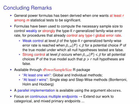
Concluding RemarksI General power formulas has been derived when one wants at least r

among m statistical tests to be significant.

I Formulas have been used to compute the necessary sample size tocontrol weakly or strongly the type-II r-generalized family-wise errorrate, for procedures that already control any type-I global error rate.

I Weak control at level β of the type-II r-generalized family-wiseerror rate is reached when βr ,m(P) 6 β for a potential choice P ofthe true model under which all null hypotheses tested are false.

I Strong control at level β occurs when βr ,m(P) 6 β for all potentialchoices P of the true model such that p > r null hypotheses arefalse.

I Available through rPowerSampleSize R packageI “At least one win”: Global and Individual methods;I “At least r wins”: Single step and Step-Wise methods (Bonferroni,

Holm and Hocberg)

I A parallel implementation is available using the argument nbcores.

I Focus on continuous multiple endpoints→ Extend our work tocategorical, and mixed primary endpoints ...

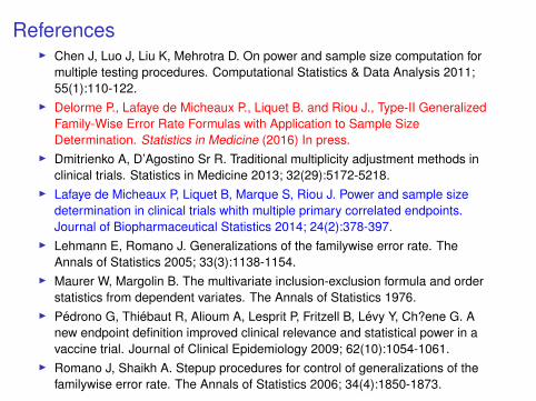
ReferencesI Chen J, Luo J, Liu K, Mehrotra D. On power and sample size computation for

multiple testing procedures. Computational Statistics & Data Analysis 2011;55(1):110-122.

I Delorme P., Lafaye de Micheaux P., Liquet B. and Riou J., Type-II GeneralizedFamily-Wise Error Rate Formulas with Application to Sample SizeDetermination. Statistics in Medicine (2016) In press.

I Dmitrienko A, D’Agostino Sr R. Traditional multiplicity adjustment methods inclinical trials. Statistics in Medicine 2013; 32(29):5172-5218.

I Lafaye de Micheaux P, Liquet B, Marque S, Riou J. Power and sample sizedetermination in clinical trials whith multiple primary correlated endpoints.Journal of Biopharmaceutical Statistics 2014; 24(2):378-397.

I Lehmann E, Romano J. Generalizations of the familywise error rate. TheAnnals of Statistics 2005; 33(3):1138-1154.

I Maurer W, Margolin B. The multivariate inclusion-exclusion formula and orderstatistics from dependent variates. The Annals of Statistics 1976.

I Pedrono G, Thiebaut R, Alioum A, Lesprit P, Fritzell B, Levy Y, Ch?ene G. Anew endpoint definition improved clinical relevance and statistical power in avaccine trial. Journal of Clinical Epidemiology 2009; 62(10):1054-1061.

I Romano J, Shaikh A. Stepup procedures for control of generalizations of thefamilywise error rate. The Annals of Statistics 2006; 34(4):1850-1873.

ANY QUESTIONS ?