TZAR TIME ZONE BASED APPROXIMATION TO RING: AN …

TZAR – TIME ZONE BASED APPROXIMATION TO RING:

AN AUTONOMOUS PROTECTION SWITCHING ALGORITHM

FOR GLOBALLY RESILIENT OPTICAL TRANSPORT NETWORKS

A THESIS SUBMITTED TO

THE GRADUATE SCHOOL OF NATURAL AND APPLIED SCIENCES

OF

MIDDLE EAST TECHNICAL UNIVERSITY

BY

FATİH DÜZGÜN

IN PARTIAL FULFILLMENT OF THE REQUIREMENTS

FOR

THE DEGREE OF MASTER OF SCIENCE

IN

ELECTRICAL AND ELECTRONICS ENGINEERING

FEBRUARY 2016

Approval of the thesis:


AN AUTONOMOUS PROTECTION SWITCHING ALGORITHM


submitted by FATİH DÜZGÜN in partial fulfillment of the requirements for the

degree of Master of Science in Electrical and Electronics Engineering

Department, Middle East Technical University by,

Prof. Dr. Gülbin Dural Ünver _________________

Dean, Graduate School of Natural and Applied Sciences

Prof. Dr. Gönül Turhan Sayan _________________

Head of Department, Electrical and Electronics Eng.

Assoc. Prof. Dr. Şenan Ece Schmidt _________________

Supervisor, Electrical and Electronics Eng. Dept., METU

Examining Committee Members:

Prof. Dr. Gözde Bozdağı Akar _________________

Electrical and Electronics Engineering Dept., METU

Assoc. Prof. Dr. Şenan Ece Schmidt _________________


Assoc. Prof. Dr. Cüneyt Bazlamaçcı _________________


Assoc. Prof. Dr. İlkay Ulusoy _________________


Assoc. Prof. Dr. Asaf Behzat Şahin _________________

Electrical and Electronics Engineering Dept., YBU

Date: February 3rd

, 2016

iv

I hereby declare that all information in this document has been obtained and

presented in accordance with academic rules and ethical conduct. I also

declare that, as required by these rules and conduct, I have fully cited and

referenced all material and results that are not original to this work.

Name, Last name : Fatih Düzgün

Signature :

v

ABSTRACT


AN AUTONOMOUS PROTECTION SWITCHING ALGORTIHM


Düzgün, Fatih

M. S., Department of Electrical and Electronics Engineering

Supervisor: Assoc. Prof. Dr. Şenan Ece Schmidt

February 2016, 109 pages

Widespread deployment of new generation high-speed networks, developments in

large capacity DWDM technologies, and continuous demand for increasingly

resilient global Internet services necessitates a revision on optical transport

networks. Considered to be one of the most promising recent phenomena in that

sense, OTN is evolving to become a major core switching platform.

In this thesis, we briefly present the progress in optical transport networking from

hardware architecture and software hierarchy points of views. Then, trends in

protection switching are pointed out through a peculiar taxonomy on computational,

topological, and efficiency aspects. Finally, an autonomous, low complexity and

inter-disciplinary (incorporating automatic protection switching of optical networks

with distance vector routing of mobile ad-hoc networks) lightpath recovery

algorithm is offered based on time-zone awareness of OTN nodes to fulfill the basic

requirements expected from mesh optical networks. The proposed algorithm is

evaluated with simulation in comparison to two well-known algorithms.

Keywords: optical transport networks, protection switching, global resilience

vi

ÖZ

TZAR – ZAMAN DİLİMİ TEMELLİ HALKA YAKLAŞIMI:

OPTİK İLETİM AĞLARININ KÜRESEL DAYANIKLILIĞI İÇİN

ÖZERK KORUMA ANAHTARLAMASI ALGORİTMASI

Düzgün, Fatih

Yüksek Lisans, Elektrik – Elektronik Mühendisliği Bölümü

Tez Yöneticisi: Asst. Prof. Dr. Şenan Ece Schmidt

Şubat 2016, 109 sayfa

Yeni nesil hızlı ağların yaygınlaşması, yüksek kapasiteli DWDM teknolojilerindeki

gelişmeler, küresel Internet servislerinin dayanıklılığını artırmaya yönelik süregelen

talepler optik iletim ağlarını yeniden gözden geçirmeyi gerektiriyor. Bu bağlamda,

güncel olguların en gelecek vadedenlerinden biri olarak değerlendirilen OTN, temel

omurga anahtarlama platformu olarak evrilmektedir.

Tezimizde, optik iletim ağlarının donanımsal mimari ve yazılımsal hiyerarşi

açılarından geldikleri nokta özetlendi. Koruma anahtarlama yöntemlerine ilişkin

hesaplama, topoloji ve verimlilik bakımından özgün bir sınıflandırma yapıldı.

Örgün optik iletim ağlarının temel gereksinimlerine cevap verebilecek nitelikte,

OTN nodlarının zaman dilimi farkındalığına dayandırılan, özerk, hesaplama

karmaşıklığı düşük ve disiplinlerarası (optik ağların otomatik koruma anahtarlaması

ile geçici mobil ağların vektörel mesafe yönlendirmesini birleştiren) bir ışıkyolu

onarım algoritması önerildi. Önerilen yöntem iki iyi bilinen algoritma ile benzetim

yoluyla karşılaştırmalı olarak değerlendirildi.

Anahtar Kelimeler: optik iletim ağları, koruma anahtarlaması, küresel dayanıklılık

vii

To my dear wife, Esra

viii

ACKNOWLEDGEMENTS

I hereby have to notify a sincere gratitude to my supervisor Assoc. Prof. Dr. Şenan

Ece Schmidt for her extremely positive guidance and constructive criticism during

this thesis studies.

I shall acknowledge time and attentiveness of our jury members Prof. Dr. Gözde

Bozdağı Akar, Assoc. Prof. Dr. Asaf Behzat Şahin, Assoc. Prof. Dr. İlkay Ulusoy,

and Assoc. Prof. Dr. Cüneyt Bazlamaçcı, without comments of whom this thesis

would not be that presentable.

I wish to express my thankfulness to Prof. Dr. Hasan Güran, Prof. Dr. Buyurman

Baykal, Prof. Dr. Cengiz Beşikçi, and Prof. Dr. İsmet Erkmen for their mental

contributions in my educational and professional career.

I would also like to thank all my family members for their lovely presence and

invaluable moral support throughout my life and continuously keen encouragement

especially for the last couple of years.

ix

TABLE OF CONTENTS

ABSTRACT ............................................................................................................... V

ÖZ ............................................................................................................................. VI

ACKNOWLEDGEMENTS .................................................................................... VIII

TABLE OF CONTENTS .......................................................................................... IX

LIST OF TABLES..................................................................................................... XI

LIST OF FIGURES .................................................................................................. XII

ABBREVIATIONS................................................................................................. XIV

CHAPTERS ............................................................................................................... 1

1. INTRODUCTION ....................................................................................... 1

1.1. Thesis Objective and Motivation ........................................................ 2

1.2. Focal Terminology ............................................................................. 4

1.3. Organization of the Thesis .................................................................. 5

2. OPTICAL TRANSPORT NETWORKS ...................................................... 7

2.1. Optical Transport Network ................................................................. 7

2.1.1 OTN Architecture ................................................................... 8

2.1.2 Encapsulation Hierarchy ......................................................... 9

2.1.3 OTN as a successor to SDH .................................................. 12

2.2 Optical Network Components .......................................................... 14

2.2.1 Optical Fiber ......................................................................... 15

2.2.2 Optical Transceivers ............................................................. 15

2.2.3 Optical Amplifiers ................................................................ 16

2.2.4 Reconfigurable Optical Add-Drop Multiplexers .................. 17

2.2.5 Optical Cross Connects ......................................................... 18

2.3 Wavelength Division Multiplexing .................................................. 18

2.4 Routing and Wavelength Assignment .............................................. 19

3. PROTECTION SWITCHING IN OTN ..................................................... 23

x

3.1. Computational Concerns .................................................................. 25

3.2. Resource Efficiency .......................................................................... 29

3.3. Topological Facts .............................................................................. 32

4. PROBLEM DEFINITION AND PROPOSED SOLUTION ...................... 39

4.1. Assumptions ..................................................................................... 39

4.2. TZAR – Time Zone based Approximation to Ring .......................... 40

4.3. Heuristics .......................................................................................... 46

5. COMPARATIVE PERFORMANCE EVALUATION .............................. 51

5.1. Definition of Packet Formats ............................................................ 51

5.2. Optical Link Model ........................................................................... 53

5.3. Processing Node Model .................................................................... 54

5.3.1. Node Model .......................................................................... 55

5.3.2. Process Model ....................................................................... 57

5.4. Simulation Scenarios ........................................................................ 62

5.4.1. Topology Definition.............................................................. 62

5.4.2. Types of Failures................................................................... 64

5.4.3. Number of Wavelengths ....................................................... 65

5.4.4. Lightpath Demand Factor ..................................................... 66

5.4.5. Algorithm Selection .............................................................. 67

5.5. Results Collected .............................................................................. 68

5.5.1. Confidence Interval ............................................................... 69

5.5.2. Blocking Probability ............................................................. 72

5.5.3. Recovery Success Ratio ........................................................ 74

5.5.4. Speed of Recovery ................................................................ 81

6. CONCLUSION .......................................................................................... 87

REFERENCES ......................................................................................................... 89

APPENDICES .......................................................................................................... 97

A. PROTECTION SWITCHING REQUIREMENTS .................................... 97

B. A SAMPLE DEMONSTRATION OF TZAR .......................................... 101

xi

LIST OF TABLES

TABLES

Table 1 – Set of ODU clients and serving OTU rates .............................................. 12

Table 2 – OTN versus SDH ..................................................................................... 14

Table 3 – Types of Optical Fiber ............................................................................. 15

Table 4 – Comparison of Optical Amplifiers ........................................................... 17

Table 5 – CWDM versus DWDM ........................................................................... 19

Table 6 – Relation of AODV with TZAR ................................................................ 46

Table 7 – TZAR Heuristics ...................................................................................... 48

Table 8 – Confidence Levels Matrix ........................................................................ 71

Table 9 – Protection Switching Algorithm Comparison .......................................... 86

xii

LIST OF FIGURES

FIGURES

Figure 1 – OTN Functional Architecture ................................................................... 8

Figure 2 – OTN Operational Architecture ................................................................. 9

Figure 3 – Optical Transport Module (OTM) .......................................................... 10

Figure 4 – Optical Line Structure Breakdown ......................................................... 11

Figure 5 – Global Internetworking Topology .......................................................... 13

Figure 6 – A sample Optical Cross Connect ............................................................ 18

Figure 7 – Protection Switching Temporal Model ................................................... 26

Figure 8 – APS Signaling Alternatives .................................................................... 27

Figure 9 - Shared Risk Groups ................................................................................. 31

Figure 10 – Alternative Protection Schemes ............................................................ 32

Figure 11 – Protection Switching in Ring Topologies ............................................. 35

Figure 12 – Alternative p-Cycle Structures .............................................................. 36

Figure 13 – Geographical correspondence of time zone with longitudes ................ 41

Figure 14 – Autonomous Systems peering at Internet Exchange Points ................. 43

Figure 15 – Content Delivery Network leasing dark fibers of Tier-1 ISPs .............. 44

Figure 16 – Time Zone based Approximation to Ring for a global mesh................ 45

Figure 17 – APS Signaling scheme for TZAR ......................................................... 47

Figure 18 – TZAR Packet Formats .......................................................................... 52

Figure 19 – DWDM Link Model ............................................................................. 53

Figure 20 – Wavelength Attribute of DWDM Links ............................................... 54

Figure 21 – Optical Cross Connect with 6 ports ...................................................... 55

Figure 22 – Verify Connectivity for OXC Module .................................................. 56

Figure 23 – Channel Table for Transmitter and Receiver Modules ......................... 56

Figure 24 – OXC Root Process Model ..................................................................... 58

Figure 25 – Child Process Model for OTN Clients .................................................. 59

xiii

Figure 26 – Child Process Model for OTN Gateways ............................................. 60

Figure 27 – Part of OXC_WSS_Parent Function Block .......................................... 61

Figure 28 – Project Startup Wizard .......................................................................... 62

Figure 29 – Rapid Configuration Tool ..................................................................... 63

Figure 30 – A Sample OTN Scenario of 10 Nodes .................................................. 64

Figure 31 – Failure Recovery Object Attributes to Schedule a Failure ................... 65

Figure 32 – Wavelengths Compound Attribute ....................................................... 65

Figure 33 – DWDM Link Model Attributes ............................................................ 66

Figure 34 – A Sample Discrete Event Simulation Sequence ................................... 66

Figure 35 – Global Attributes Configuration in a Simulation Set ........................... 67

Figure 36 – Manage Scenarios Screen ..................................................................... 68

Figure 37 – DES Execution Manager Window ........................................................ 68

Figure 38 – Sources for Stochastic Behavior ........................................................... 70

Figure 39 – Blocking Probability vs Number of Wavelengths (distribution) .......... 72

Figure 40 – Blocking Probability vs Number of Wavelengths (mean values) ........ 73

Figure 41 – Blocking Probability vs Number of Wavelengths (confidence) ........... 73

Figure 42 – Recovery Success Ratio vs Lightpath Demand .................................... 74

Figure 43 – Recovery Success Ratio vs Number of Wavelengths ........................... 76

Figure 44 – Recovery Success Ratio vs Number of Nodes ..................................... 79

Figure 45 – Average Recovery Time vs Number of Nodes ..................................... 82

Figure 46 – TZAR Demonstration Phase 1 ............................................................ 101









xiv

ABBREVIATIONS

AODV Ad-hoc On-demand Distance Vector

AON All Optical Networks

APS Automatic Protection Switching

AS Autonomous System

ASE Amplified Spontaneous Emission

ASON Automatically Switched Optical Networks

ATM Asynchronous Transfer Mode

BLSR Bidirectional Line-Switched Rings

BGP Border Gateway Protocol

CD Chromatic Dispersion

CDN Content Delivery Network

CWDM Coarse Wavelength Division Multiplexing

DBPP Dedicated Backup Path Protection

DWDM Dense Wavelength Division Multiplexing

EDFA Erbium Doped Fiber Amplifier

FC Fibre Channel

FCAPS Fault, Configuration, Accounting, Performance, and Security

FTTX Fiber to the X, where x can be home, building or curb

GbE Gigabit Ethernet

GMPLS Generalized MPLS

GPS Global Positioning System

HAMP Hamiltonian p-Cycle

ICT Information and Communications Technologies

IP Internet Protocol

ISP Internet Services Provider

IT Information Technologies

xv

ITU International Telecommunication Union

ITU-T Telecommunication Standardization Sector of ITU

IXP Internet Exchange Point

KSPF k-Shortest Path First

MAN Metropolitan Area Network

MANET Mobile Ad-hoc Networks

MPLS Multiprotocol Label Switching

MTTF Mean Time To Failure

NTP Network Time Protocol

OAM Operations, Administration, and Maintenance

OCC Optical Carrier Channel

OCh Optical Channel

ODU OCh Data Unit

OEO Optical-Electrical-Optical

OH Overhead

OMS Optical Multiplex Section

OOS OTM Overhead Signal

OPU OCh Payload Unit

OSNR Optical Signal to Noise Ratio

OTN Optical Transport Network

OTM Optical Transport Module

OTS Optical Transmission Section

OTU OCh Transport Unit

OXC Optical Cross Connect

PMD Polarization Mode Dispersion

PON Passive Optical Network

POP Point Of Presence

PXC Photonic Cross Connect

PXT Pre-Cross-Connected Trails

ROADM Reconfigurable Optical Add-Drop Multiplexer

ROW Right Of Way

RR Reverse Request

xvi

RWA Routing and Wavelength Assignment

SBPP Shared Backup Path Protection

SD Signal Degrade

SDH Synchronous Digital Hierarchy

SF Signal Fail

SLA Service Level Agreement

SOA Semiconductor Optical Amplifier

SONET Synchronous Optical Network

SRG Shared Risk Group

SRLG Shared Risk Link Group

SRNG Shared Risk Node Group

TZAR Time Zone based Approximation to Ring

UPSR Unidirectional Path-Switched Rings

UTC Coordinated Universal Time

WAN Wide Area Network

WDM Wavelength Division Multiplexing

WSS Wavelength Selective Switch

1

CHAPTER 1

INTRODUCTION

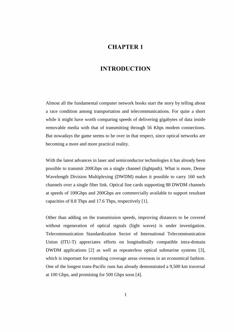
Almost all the fundamental computer network books start the story by telling about

a race condition among transportation and telecommunications. For quite a short

while it might have worth comparing speeds of delivering gigabytes of data inside

removable media with that of transmitting through 56 Kbps modem connections.

But nowadays the game seems to be over in that respect, since optical networks are

becoming a more and more practical reality.

With the latest advances in laser and semiconductor technologies it has already been

possible to transmit 200Gbps on a single channel (lightpath). What is more, Dense

Wavelength Division Multiplexing (DWDM) makes it possible to carry 160 such

channels over a single fiber link. Optical line cards supporting 88 DWDM channels

at speeds of 100Gbps and 200Gbps are commercially available to support resultant

capacities of 8.8 Tbps and 17.6 Tbps, respectively [1].

Other than adding on the transmission speeds, improving distances to be covered

without regeneration of optical signals (light waves) is under investigation.

Telecommunication Standardization Sector of International Telecommunication

Union (ITU-T) appreciates efforts on longitudinally compatible intra-domain

DWDM applications [2] as well as repeaterless optical submarine systems [3],

which is important for extending coverage areas overseas in an economical fashion.

One of the longest trans-Pacific runs has already demonstrated a 9,500 km traversal

at 100 Gbps, and promising for 500 Gbps soon [4].

2

1.1. Thesis Objective and Motivation

Networks are being constructed in a hierarchy to comply with the demand

characteristics of varying scopes. Access networks provide last mile connectivity to

clients for up to tens of km. Metropolitan Area Networks (MAN) serve as a

distribution layer within specific countries typically in a sub-1000 km range.

Transport networks constitute the core international/intercontinental Wide Area

Network (WAN) to provide global reach through interconnectivity among Tier1 and

Tier2 ISP domains.

During 1990s fiber optic systems started to dominate long-haul transmission for

WAN linear trails. Then in 2000s Synchronous Digital Hierarchy (SDH) and

Synchronous Optical Network (SONET) infrastructure matured the services for

MAN rings. And recently by 2010s Passive Optical Networks (PON) are being

deployed to provide full wavelength access through star or bus FTTX (Fiber to the

x, where x can be home, office, building or curb) topologies.

Hence, optical networking has eventually become a much more visible instrument

of our era. As Internet continues to evolve with many new bandwidth-hungry

applications (such as video on demand, cloud computing and social media) and

clients (such as smart phones/TVs and tablets) on top of it, huge traffic consumption

is expected to bounce back from access (PON) to distribution (MAN) and core

(WAN) networks [5].

To cope with such an aggressive demand, transport protocols will have to adapt to

efficient use of DWDM links for higher levels of throughput and reliability. That is

why core players of global Internet industry are concentrating and investing more

on optical networking both in terms of active equipment [6], and cabling

infrastructure [7]. Electronic router market leaders tend to merge with smaller-size

pure optical technology developers, while best circuit switching implementers

change their strategies to provide routed packets a new media [8].

3

Nevertheless, whatever developments will be done to increase performance on

active equipment, 70% of network downtime will continue to be related to physical

layer [9]. There are three major categories of physical failure sources, examples of

which are detailed in [10]:

I. Unfortunate natural disasters – floods, earthquakes, etc. (An earthquake with

aftershocks continuing for the next two days took place in 26 December

2006 near Taiwan. Submarine cables connecting Asia to North America

were damaged. Internet capacity of China was reduced to 26 %.)

II. Unintentional accidents – construction digging faults, human errors in cord

patching, etc. (A train derailed into a tunnel in 18 July 2001 in Baltimore,

which is one of the most critical ports for transoceanic fiber optic cabling

infrastructure in the Northeast United States. Resulting fire caused backbone

link failures for 7 major ISPs.)

III. Intentional cyber-attacks – well planned cable cuts approaching to or

emanating from a targeted victim (In January 2008 Internet connectivity of

most of Arabian Peninsula countries were tested via a series of cable cuts in

the Mediterranean Sea and Indian Ocean. More than 20 million clients were

suffered.)

Whenever such catastrophic events happen in physical layer, switching and routing

layers in sequence try to recover whole network services from the failed state.

However, uncorrelated nature and the random behavior of such failures make it

quite difficult to handle them at upper layers. For the above mentioned examples;

Taiwan 2006 – Although BGP was able to recover some part of the network,

traffic between Taiwan and China had to traverse Pacific Ocean twice until

manual traffic engineering was done.

Baltimore 2001 – Although most of the traffic was rerouted on alternative

links, overall network slowdown and the congestion could only be avoided

within 36 hours after new cables were laid to restore the failed physical

capacity.

4

As a result, highly realistic protection switching mechanisms should be deployed in

optical transport networks to recover from any scenario in an immediate manner.

This thesis offers a new approach, which we call “Time-Zone based Approximation

to Ring” (TZAR), to improve autonomous resilience of globally distributed OTN

over mesh topologies. Time zone parameter not only acts as a cross-layer carrier of

geo-location information, but also a diversity guarantee among primary and

protection (backup) lightpaths.

1.2. Focal Terminology

While focusing on resilience in OTN throughout this thesis, we will be using special

terms, some of which are necessary to clarify from the very beginning:

Resilience; is the ability of a network to provide accepted level of services

even after physical failures or operational faults. When used in the context

of networking, “survivability” has the same meaning.

Protection; is a resilience mechanism, in which backup resources are

provisioned with the primary services during initial network setup, i.e.

before any failures or faults happen.

Restoration; is a resilience mechanism, in which backup resources for the

affected traffic patterns are computed and configured dynamically right after

the detection of any failure or faults.

Lightpath; is a two-tuple (P,λ), where P represents a path (a sequence of

links connecting neighboring nodes) from a source to a destination and λ

represents the wavelength(s) associated with each link along that P.

Diversity; is a feature of at least two lightpaths. The less network resources

these lightpaths share, the more diverse they are. Ideal diversity of primary

and backup lightpaths for a specific connection is achieved, when they do

not share any links or nodes other than the communicating end points.

Protection Switching; is the operation performed at Data Link Layer

(Layer-2) to recover failed services via switching on to a pre-computed, pre-

configured, and/or pre-established connection.

5

Route Restoration; is the operation performed at Network Layer (Layer-3)

to recover failed services either via rerouting through a backup route, or by

invoking a new routing process.

Although there may be different understandings in literature, we believe that the

above descriptions are in line with the philosophy of ones given in relevant ITU-T

standards. Technical details and inter-relations of all these terms will be studied in

the following chapters as outlined below.

1.3. Organization of the Thesis

Starting with a brief introduction on Optical Transport Networks (OTN), we first

summarize state of the art components of All Optical Networks (AONs), physical

details of Wavelength Division Multiplexing (WDM), and principles of Routing

and Wavelength Assignment (RWA) techniques.

In the third chapter a critical discussion on the Protection Switching algorithms

offered and the performance metrics evaluated so far is presented. Then in the

fourth chapter, we introduce a new approach (TZAR) based on Time-Zone

parameter along with the assumptions made and benefits expected.

In the fifth chapter, after a description of simulation environment and data

collection tools used in our analysis, simulation scenarios and results collected are

detailed to evaluate the performance of TZAR in terms of optical path resiliency

and service restoration times.

At the end of the thesis, we will conclude with a summary of our major

contributions and suggestions for a couple of future works to be investigated

further. Appendix A is also provided as a benchmark to check for the applicability

of our new protection switching protocol.

6

7

CHAPTER 2

OPTICAL TRANSPORT NETWORKS

Optical Transport Network (OTN) is one of the most promising recent phenomena

in networking industry. Regardless of the applications and appliances pushed into

the Internet access market, OTN is expected to present the necessary core transport

services in an efficient and granular manner.

Though OTN has to be considered in numerous dimensions, for the sake of

simplicity we will be squeezing our scope to the standards published, key hardware

components, physical state of optical communications, and the software restrictions

on service provisioning.

2.1. Optical Transport Network

For decades voice-centric circuit switching networks and data-centric packet

routing networks were operated by service providers in parallel. By the beginning

of third millennium, sophistication of cloud computing, mobile applications, and

multimedia services introduced a new transport network optimization demand to

handle modern traffic patterns and content on a unified platform.

Thanks to the availability of Wavelength Division Multiplexing (WDM)

technologies, OTN is then defined as a payload-transparent lightpath management

infrastructure by Telecommunications Standardization Sector of International

Telecommunications Union (ITU-T) with a series of recommendations, such as

[11], [12], and [13].

8

2.1.1 OTN Architecture

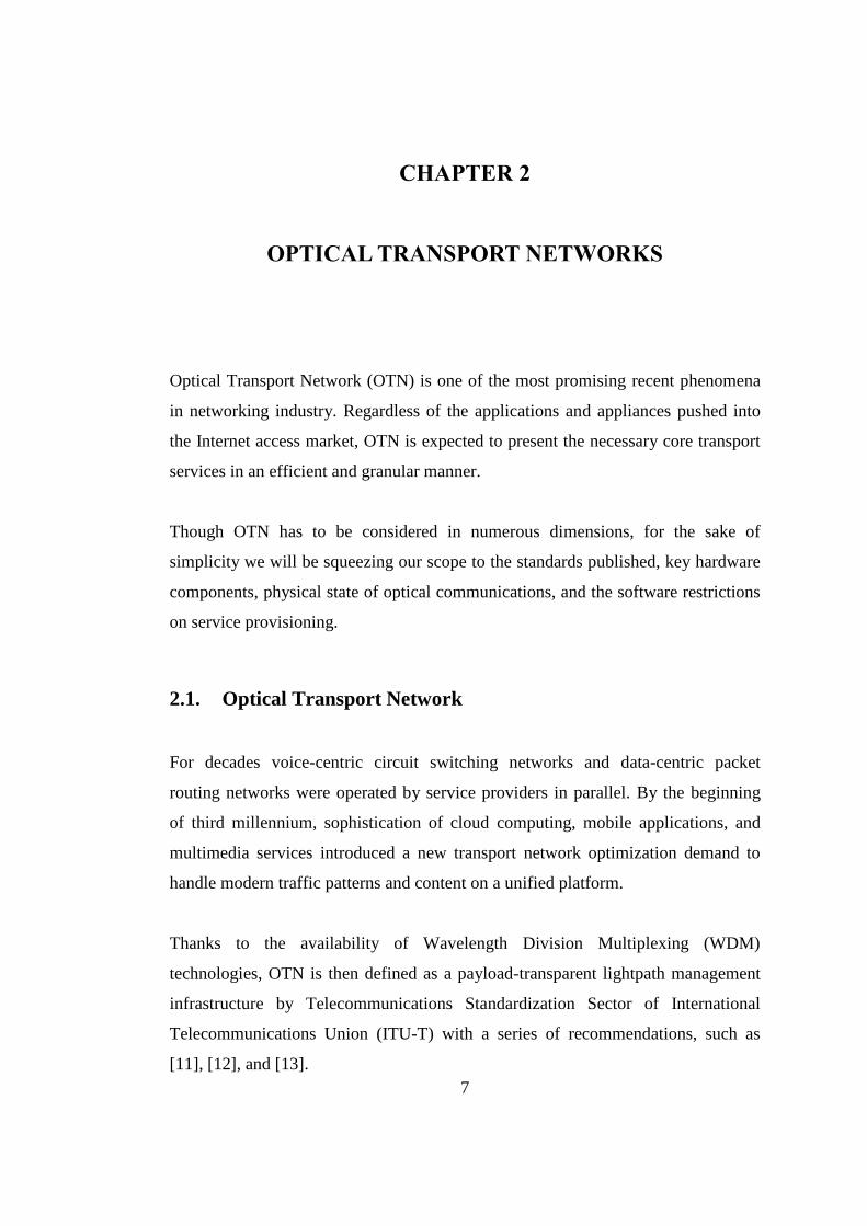
As illustrated in Figure 1, OTN is designed to function as a digital wrapper. It takes

optical signals generated by any upper layer services, and bundle them on specific

wavelengths in a DWDM system. This feature not only provides backward

compatibility with all the existing WAN protocols and equipment running them, but

also utilizes each wavelength with as many services as the line rate allows

asynchronously for achieving the best possible spectral efficiency. Details of how

OTN interfaces with upper layer services and how client signals are mapped on to

the OTN framing structure are given in [11].

OTN

Wrapper

Optical Transport Network Domain

DWDM Ligthpaths

Digital Circuits

Packet Networks

Service Applications

(Internet, Mobile, Video, Storage)

IP

SO

NE

T /

SD

H

Fib

re C

han

nel

Car

rier

Eth

ernet

MP

LS

OT

N

STM-256

10GbE

8GFC

2GBps

SDH

Ethernet

Fibre Channel

CBR Service

a. b.

Figure 1 – OTN Functional Architecture: a. Protocol Stack, b. Digital Wrapper

Once OTN is populated with critical amount of services and data; operations,

administration, and maintenance (OAM) of the network as well as fault,

configuration, accounting, performance, and security (FCAPS) features of client

payload have to be satisfied. A generic architecture in that respect is recommended

in [12].

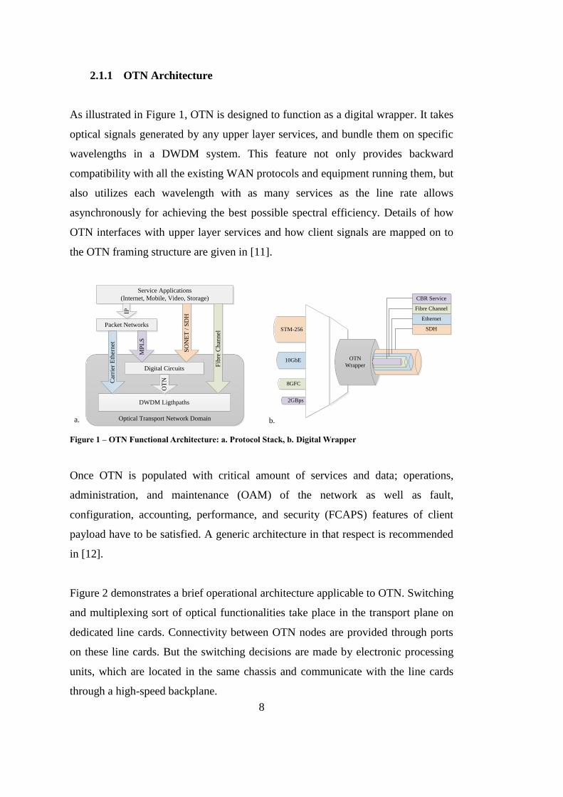
Figure 2 demonstrates a brief operational architecture applicable to OTN. Switching

and multiplexing sort of optical functionalities take place in the transport plane on

dedicated line cards. Connectivity between OTN nodes are provided through ports

on these line cards. But the switching decisions are made by electronic processing

units, which are located in the same chassis and communicate with the line cards

through a high-speed backplane.

9

Transport Plane

Control Plane

Man

agem

ent

Pla

ne

Transmission Line Cards

Processing Controllers

Configuration

& Signalling

Field Information

(Topology & Alarms)

Transmission Line Cards

MDS 9506

STATUSFAN

2

1

3

4

5

6

CONSOLE

MGMT

10/100 COM2

STA

TUS

SY

STE

M

AC

TIV

E

PW

R M

GM

T

RE

SE

T CF

SUPERVISOR

WS-X9530-SFI

CONSOLE

MGMT

10/100 COM2

STA

TUS

SY

STE

M

AC

TIV

E

PW

R M

GM

T

RE

SE

T CF

SUPERVISOR

WS-X9530-SFI

CONSOLE

WS-SUP720

SUPERVISOR 720 WITH INTEGRATED SWITCH FABRIC

PWR

MGM

TACTIV

E

SYSTEM

STATU

S E J E C T

E J E C TLI

NK

LINK

LINK

RESET

Disk 0

Disk 1

Port 1

Port 2

CONSOLE

WS-SUP720

SUPERVISOR 720 WITH INTEGRATED SWITCH FABRIC

PWR

MGM

TACTIV

E

SYSTEM

STATU

S E J E C T

E J E C TLI

NK

LINK

LINK

RESET

Disk 0

Disk 1

Port 1

Port 2

STATUS

10 Gbps FC Module

DS-X9704

1

LINK

2

LINK

3

LINK

4

LINK

STATUS

10 Gbps FC Module

DS-X9704

1

LINK

2

LINK

3

LINK

4

LINK

1 2 3 4 5 6 7 8

STATUS

LINK - - SPEED LINK -LINK - - SPEED

13 14 15 16

LINK - - SPEED

9 10 11 12

- SPEED

WS-X9016

1/2G FC Module

1 2 3 4 5 6 7 8

STATUS

LINK - - SPEED LINK -LINK - - SPEED

13 14 15 16

LINK - - SPEED

9 10 11 12

- SPEED

WS-X9016

1/2G FC Module

Figure 2 – OTN Operational Architecture

Processing controllers, which constitute the control plane, can either perform

decisions autonomously via probing local transmission line cards and collecting

information from neighboring nodes, or receive commands from a set of

management hosts. Both of these communications are performed through a

supervisory channel available in the encapsulation hierarchy (to be discussed in the

next sub-section) of OTN.

Being responsible for the OAM and FCAPS features, management plane has to

coordinate fixed hosts and mobile engineers. Harmonizing the signaling and alarms

on fixed hosts with the field information regarding environmental situation and

physical layout (such as equipment placement within cabinets and cable installation

along the path) received from mobile engineers, control plane is configured by

management plane.

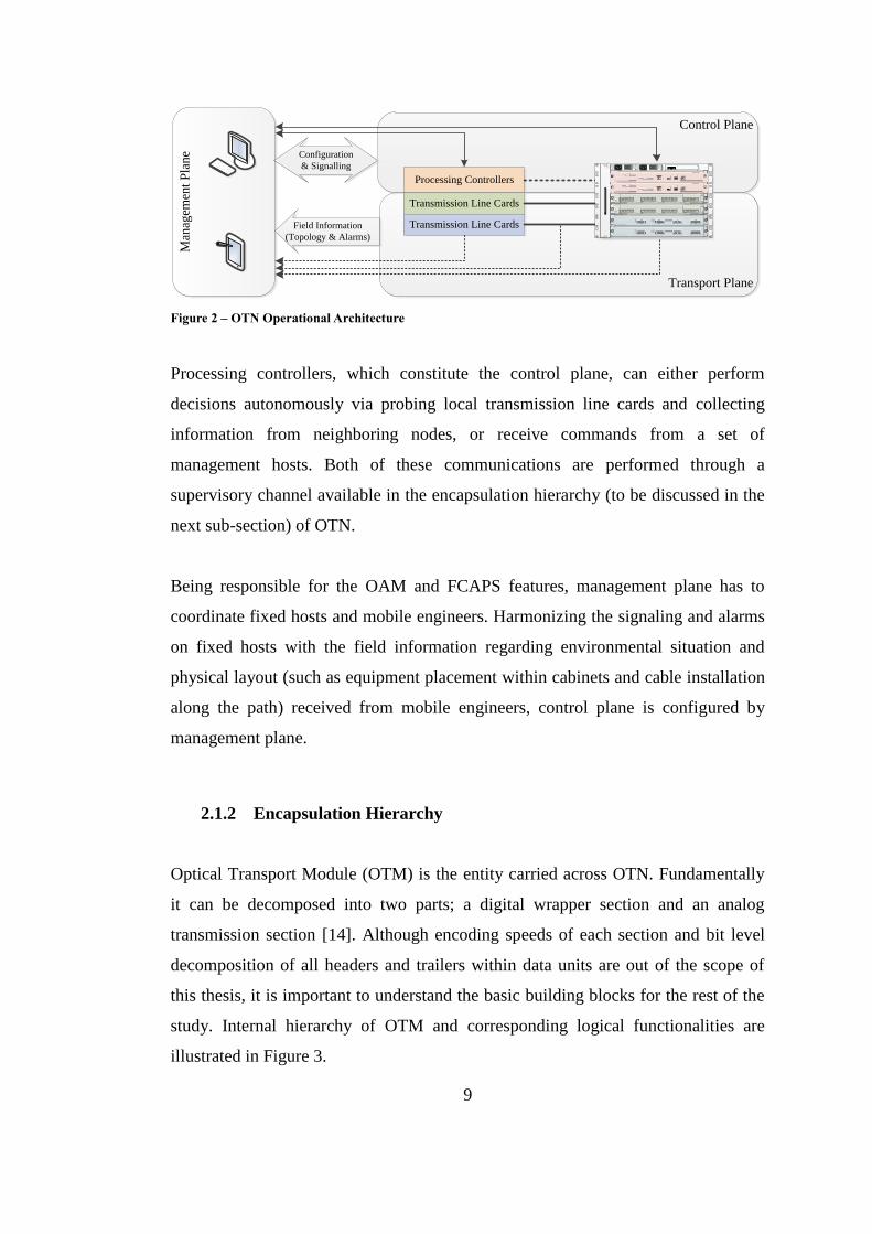
2.1.2 Encapsulation Hierarchy

Optical Transport Module (OTM) is the entity carried across OTN. Fundamentally

it can be decomposed into two parts; a digital wrapper section and an analog

transmission section [14]. Although encoding speeds of each section and bit level

decomposition of all headers and trailers within data units are out of the scope of

this thesis, it is important to understand the basic building blocks for the rest of the

study. Internal hierarchy of OTM and corresponding logical functionalities are

illustrated in Figure 3.

10

Optical channel Payload Unit (OPU) presents the client services, such as

ATM, GbE, FC, and SDH. OPU overhead (OH) defines the payload type.

Optical channel Data Unit (ODU) provides end-to-end path supervision in

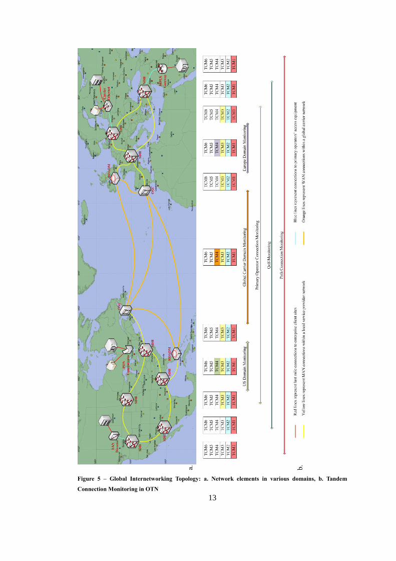
terms of switching and multiplexing control. ODU OH includes Path

Monitoring (PM) field to check for the multiplex section performance and

six Tandem Connection Monitoring (TCM) fields to let path monitoring

functionalities managed by different ISP domains in nested, overlapping,

and cascaded topologies as demonstrated in Figure 5.b.

Optical channel Transport Unit (OTU) conditions the signal transmitted via

3R – retiming, reshaping, and regeneration. Section Monitoring (SM) field

in OTU OH is basically used for alignment between OTN hops. General

Communication Channel (GCC) bytes are used as a supporter to protection

switching, service-level reporting, and control plane communications

signaling. Another critical functionality, which is a distinction of OTN when

compared to SDH, is provided by Forward Error Control (FEC) trailer in

OTU. Reed-Solomon RS(255,239) code, where 16 bytes of overhead data is

added to each 239 bytes of payload data, is used to detect 16 symbol errors

or to correct 8 symbol errors in any code word [15].

A

nal

og

Optical Transmission Section (OTS)

Optical Multiplex Section (OMS)

Optical Channel (OCh)

OCC OCC OCCOptical Carrier Channel (OCC)

Dig

ital

OCh Transport Unit (OTU)

OCh Data Unit (ODU)

Client Data

OCh Payload Unit (OPU)OPU

OH

ODU

OH

OTU

OH FEC

AdaptationAdaptation

OT

M O

ver

hea

d S

ign

al (

OO

S)

OCC

OH

OCC

OH

OCh

OH

OCC

OH

OCC

OH

OMS

OH

OTS

OH

Transmission

Switching and Multiplexing

Management

Client Service Mapping

Figure 3 – Optical Transport Module (OTM) [14]

11

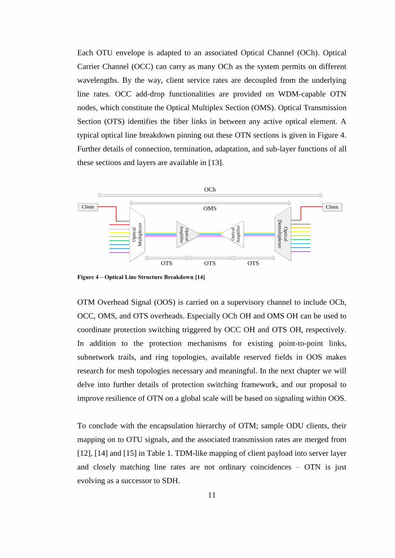
Each OTU envelope is adapted to an associated Optical Channel (OCh). Optical

Carrier Channel (OCC) can carry as many OCh as the system permits on different

wavelengths. By the way, client service rates are decoupled from the underlying

line rates. OCC add-drop functionalities are provided on WDM-capable OTN

nodes, which constitute the Optical Multiplex Section (OMS). Optical Transmission

Section (OTS) identifies the fiber links in between any active optical element. A

typical optical line breakdown pinning out these OTN sections is given in Figure 4.

Further details of connection, termination, adaptation, and sub-layer functions of all

these sections and layers are available in [13].

Client

Op

tica

l

Am

pli

fier

Client

Op

tical

Dem

ultip

lexer

OTS OTS OTS

OMS

OCh

Op

tica

l

Mu

ltip

lex

er Op

tical

Am

plifier

Figure 4 – Optical Line Structure Breakdown [14]

OTM Overhead Signal (OOS) is carried on a supervisory channel to include OCh,

OCC, OMS, and OTS overheads. Especially OCh OH and OMS OH can be used to

coordinate protection switching triggered by OCC OH and OTS OH, respectively.

In addition to the protection mechanisms for existing point-to-point links,

subnetwork trails, and ring topologies, available reserved fields in OOS makes

research for mesh topologies necessary and meaningful. In the next chapter we will

delve into further details of protection switching framework, and our proposal to

improve resilience of OTN on a global scale will be based on signaling within OOS.

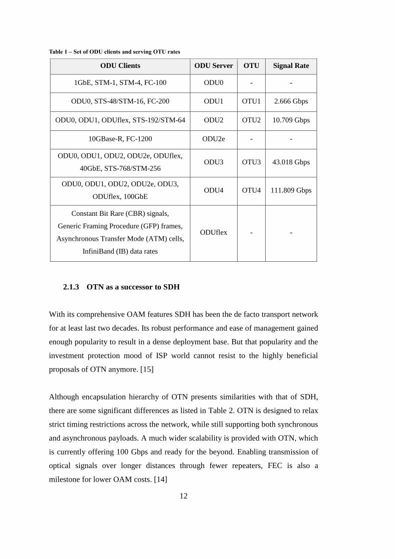
To conclude with the encapsulation hierarchy of OTM; sample ODU clients, their

mapping on to OTU signals, and the associated transmission rates are merged from

[12], [14] and [15] in Table 1. TDM-like mapping of client payload into server layer

and closely matching line rates are not ordinary coincidences – OTN is just

evolving as a successor to SDH.

12

Table 1 – Set of ODU clients and serving OTU rates

ODU Clients ODU Server OTU Signal Rate

1GbE, STM-1, STM-4, FC-100 ODU0 - -

ODU0, STS-48/STM-16, FC-200 ODU1 OTU1 2.666 Gbps

ODU0, ODU1, ODUflex, STS-192/STM-64 ODU2 OTU2 10.709 Gbps

10GBase-R, FC-1200 ODU2e - -

ODU0, ODU1, ODU2, ODU2e, ODUflex,

40GbE, STS-768/STM-256 ODU3 OTU3 43.018 Gbps

ODU0, ODU1, ODU2, ODU2e, ODU3,

ODUflex, 100GbE ODU4 OTU4 111.809 Gbps

Constant Bit Rare (CBR) signals,

Generic Framing Procedure (GFP) frames,

Asynchronous Transfer Mode (ATM) cells,

InfiniBand (IB) data rates

ODUflex - -

2.1.3 OTN as a successor to SDH

With its comprehensive OAM features SDH has been the de facto transport network

for at least last two decades. Its robust performance and ease of management gained

enough popularity to result in a dense deployment base. But that popularity and the

investment protection mood of ISP world cannot resist to the highly beneficial

proposals of OTN anymore. [15]

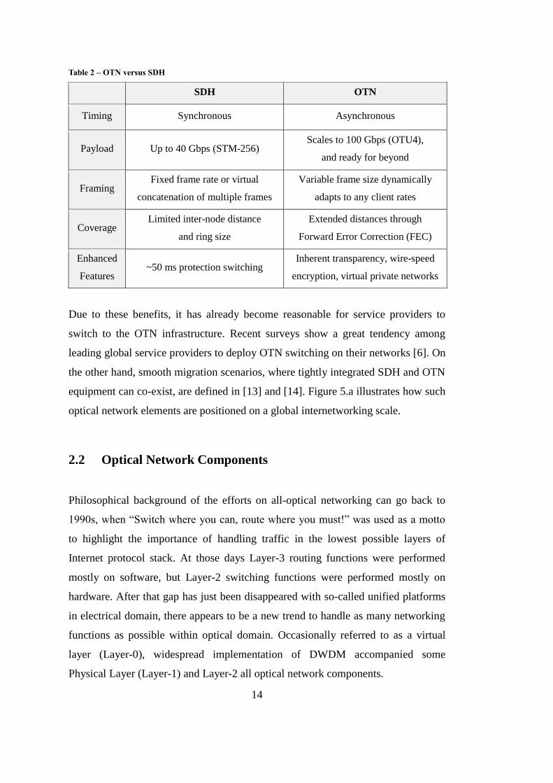
Although encapsulation hierarchy of OTN presents similarities with that of SDH,

there are some significant differences as listed in Table 2. OTN is designed to relax

strict timing restrictions across the network, while still supporting both synchronous

and asynchronous payloads. A much wider scalability is provided with OTN, which

is currently offering 100 Gbps and ready for the beyond. Enabling transmission of

optical signals over longer distances through fewer repeaters, FEC is also a

milestone for lower OAM costs. [14]

13

Figure 5 – Global Internetworking Topology: a. Network elements in various domains, b. Tandem

Connection Monitoring in OTN

14

Table 2 – OTN versus SDH

SDH OTN

Timing Synchronous Asynchronous

Payload Up to 40 Gbps (STM-256) Scales to 100 Gbps (OTU4),

and ready for beyond

Framing Fixed frame rate or virtual

concatenation of multiple frames

Variable frame size dynamically

adapts to any client rates

Coverage Limited inter-node distance

and ring size

Extended distances through

Forward Error Correction (FEC)

Enhanced

Features ~50 ms protection switching

Inherent transparency, wire-speed

encryption, virtual private networks

Due to these benefits, it has already become reasonable for service providers to

switch to the OTN infrastructure. Recent surveys show a great tendency among

leading global service providers to deploy OTN switching on their networks [6]. On

the other hand, smooth migration scenarios, where tightly integrated SDH and OTN

equipment can co-exist, are defined in [13] and [14]. Figure 5.a illustrates how such

optical network elements are positioned on a global internetworking scale.

2.2 Optical Network Components

Philosophical background of the efforts on all-optical networking can go back to

1990s, when “Switch where you can, route where you must!” was used as a motto

to highlight the importance of handling traffic in the lowest possible layers of

Internet protocol stack. At those days Layer-3 routing functions were performed

mostly on software, but Layer-2 switching functions were performed mostly on

hardware. After that gap has just been disappeared with so-called unified platforms

in electrical domain, there appears to be a new trend to handle as many networking

functions as possible within optical domain. Occasionally referred to as a virtual

layer (Layer-0), widespread implementation of DWDM accompanied some

Physical Layer (Layer-1) and Layer-2 all optical network components.

15

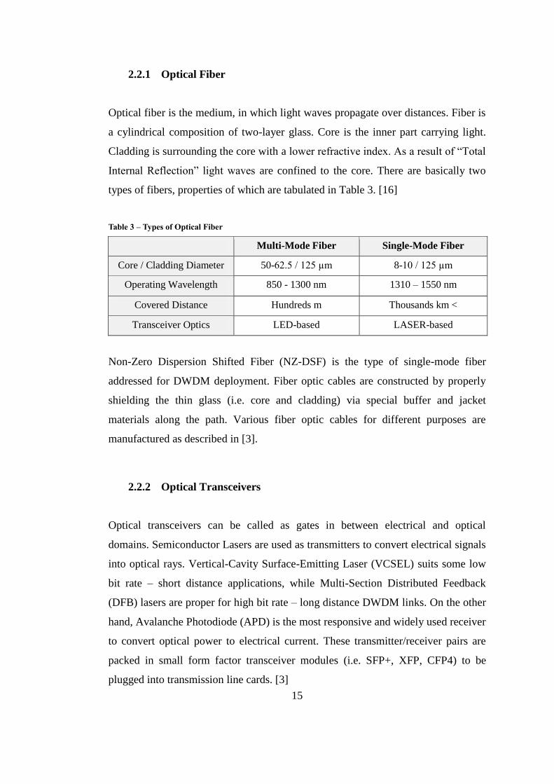
2.2.1 Optical Fiber

Optical fiber is the medium, in which light waves propagate over distances. Fiber is

a cylindrical composition of two-layer glass. Core is the inner part carrying light.

Cladding is surrounding the core with a lower refractive index. As a result of “Total

Internal Reflection” light waves are confined to the core. There are basically two

types of fibers, properties of which are tabulated in Table 3. [16]

Table 3 – Types of Optical Fiber

Multi-Mode Fiber Single-Mode Fiber

Core / Cladding Diameter 50-62.5 / 125 µm 8-10 / 125 µm

Operating Wavelength 850 - 1300 nm 1310 – 1550 nm

Covered Distance Hundreds m Thousands km <

Transceiver Optics LED-based LASER-based

Non-Zero Dispersion Shifted Fiber (NZ-DSF) is the type of single-mode fiber

addressed for DWDM deployment. Fiber optic cables are constructed by properly

shielding the thin glass (i.e. core and cladding) via special buffer and jacket

materials along the path. Various fiber optic cables for different purposes are

manufactured as described in [3].

2.2.2 Optical Transceivers

Optical transceivers can be called as gates in between electrical and optical

domains. Semiconductor Lasers are used as transmitters to convert electrical signals

into optical rays. Vertical-Cavity Surface-Emitting Laser (VCSEL) suits some low

bit rate – short distance applications, while Multi-Section Distributed Feedback

(DFB) lasers are proper for high bit rate – long distance DWDM links. On the other

hand, Avalanche Photodiode (APD) is the most responsive and widely used receiver

to convert optical power to electrical current. These transmitter/receiver pairs are

packed in small form factor transceiver modules (i.e. SFP+, XFP, CFP4) to be

plugged into transmission line cards. [3]

16

2.2.3 Optical Amplifiers

When it comes to traversing terrestrial and submarine links, amplification of the

carrier signal in optical domain without any OEO (optical to electronic and from

electronic back to optical) conversions has become a must. On transmitter side,

sending the data with maximum available power so as to reach the farthest next hop

has no any detrimental effects. On receiver side though, a rather attenuated signal

would be much safer [16]. However, too much attenuation would result in

unacceptable bit error rates (BER) because of the noise introduced on the way. To

provide more or less reasonable signal levels throughout the transmission link

following optical amplifiers are developed:

Erbium Doped Fiber Amplifier (EDFA); utilizes quantum properties of

rare-earth Erbium ions (Er3+), which perfectly matches the low loss region

of conventional (C band) and long wavelength (L band) telecom bands.

EDFA operates via a pump laser, which is mixed with the input signal

through a coupler. In the active medium Erbium ions are excited to higher

energy levels. Some of the signal photons collide with these excited ions and

cause stimulated emission. This action is the main source of signal

amplification, since signal photons are doubled with each such collision.

Gains on the order of 40 dB (10,000 photons out per photon in!) or more can

be achieved with such EDFA architectures. [17]

Semiconductor Optical Amplifier (SOA); uses electrons in the active

medium, which are excited electrically by a pump (if it is correct to say so)

current. Since upper-state life-time is rather short, lower energy can be

stored. And amplifier responds to pump power much more quickly (on the

order of hundred picoseconds). [18]

Raman Amplifiers; are also known as distributed amplifiers because of

their intrinsic behavior, which can take place on installed single-mode fiber

base. The principle behind their operation is stimulated Raman scattering.

They best perform with counter-propagating pump light on the receiver side,

and by the way they can be perfect complementary for EDFA. [3]

17

Table 4 – Comparison of Optical Amplifiers

EDFA SOA Raman

Gain (dB) >40 >30 >25

Waveband (nm) 1530-1560 1280-1650 1280-1650

Polarization No No Yes

Dispersion No Yes Yes

Size Rack-mount Chip-scale Moderate

Cost Factor Moderate Low High

Table 4 provides a comparative summary of available optical amplifier types.

EDFA is suitable to be used as a booster amplifier right after a transmitting end or

as a line amplifier in the middle of long haul multiplex sections. Raman is a natural

pre-amplifier to be positioned just before a receiving end. With its low cost and

small size SOA is an option to be considered within transceiver modules circuitry.

2.2.4 Reconfigurable Optical Add-Drop Multiplexers

Multiplexing is to combine multiple colors of light waves into a single fiber.

Demultiplexing is to split a light wave back into multiple colors. Shortly referred as

MUX/DMUX, multiplexer and demultiplexer modules are simple prism-like units.

Based on MUX/DMUX units, Reconfigurable Optical Add-Drop Multiplexer

(ROADM) selectively adds and drops certain wavelengths within a DWDM

channel. Not to disturb wavelengths passing through, following internal

components are used while doing these add-drop operations: [16]

Fiber Bragg Grating (FBG); is an optical bandpass filter used to reflect

selected wavelengths.

Circulator; is a 3-port fiber, where light coming from ports 1 and 2 goes out

from 2 and 3, respectively.

Splitter; is a tap to split optical signal into two. 50/50 splitter is used for

protection switching, while 99/1 is used for optical performance monitoring.

18

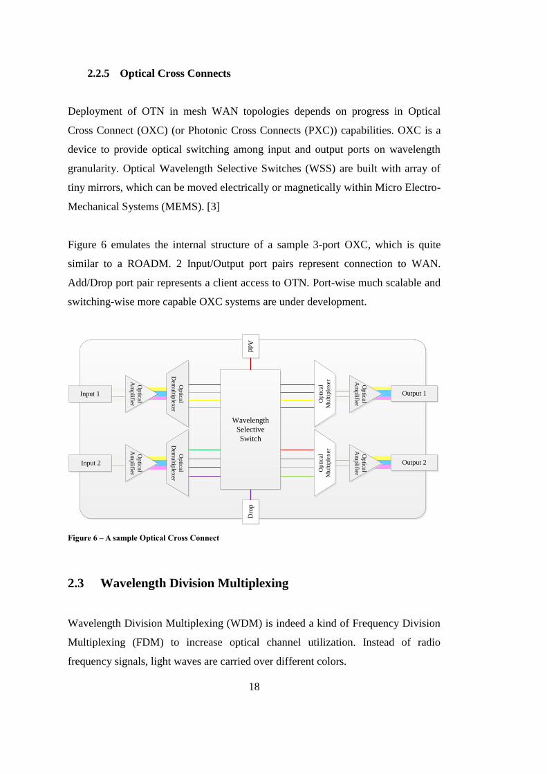
2.2.5 Optical Cross Connects

Deployment of OTN in mesh WAN topologies depends on progress in Optical

Cross Connect (OXC) (or Photonic Cross Connects (PXC)) capabilities. OXC is a

device to provide optical switching among input and output ports on wavelength

granularity. Optical Wavelength Selective Switches (WSS) are built with array of

tiny mirrors, which can be moved electrically or magnetically within Micro Electro-

Mechanical Systems (MEMS). [3]

Figure 6 emulates the internal structure of a sample 3-port OXC, which is quite

similar to a ROADM. 2 Input/Output port pairs represent connection to WAN.

Add/Drop port pair represents a client access to OTN. Port-wise much scalable and

switching-wise more capable OXC systems are under development.

Ad

d

Dro

p

Input 1

Op

tical

Am

plifier

Op

tical

Am

plifier

Output 1

Op

tical

Dem

ultip

lexer

Op

tica

l

Mu

ltip

lex

er

Input 2

Op

tical

Am

plifier

Op

tical

Am

plifier

Output 2

Op

tical

Dem

ultip

lexer

Op

tica

l

Mu

ltip

lex

er

Wavelength

Selective

Switch

Figure 6 – A sample Optical Cross Connect

2.3 Wavelength Division Multiplexing

Wavelength Division Multiplexing (WDM) is indeed a kind of Frequency Division

Multiplexing (FDM) to increase optical channel utilization. Instead of radio

frequency signals, light waves are carried over different colors.

19

There are basically two types of WDM applications – Coarse WDM (CWDM) and

Dense WDM (DWDM), spectral properties of which are given in [19] and [20],

respectively. Although underlying physical principles are the same for both CWDM

and DWDM, they have different implementations as outlined in Table 5.

Table 5 – CWDM versus DWDM

CWDM DWDM

Spectral Band 1271 – 1611 nm 1530 – 1625 nm

Channel Spacing 20 nm < 12.5 / 25 / 50 / 100 GHz

0.1 / 0.2 / 0.4 / 0.8 nm

Number of Channels 8 Channels are possible

in 160 nm of spectrum

160 Channels are possible

in 32 nm of spectrum

Implementation

Cheaper uncooled lasers,

Telecom band multiplexing

on to a single-strand fiber

Stays in C and L telecom

bands, Works with EDFA

in long haul systems

2.4 Routing and Wavelength Assignment

In optical domain connections refer to lightpaths, and corresponding connection

requests can be handled not only by finding a physical path from source to

destination, but also by assigning an appropriate wavelength. This is the most

primitive definition of Routing and Wavelength Assignment (RWA). As the

definition inspires, problem can be decomposed into two steps [21]:

i. Routing; to identify an appropriate path between source (S) and destination

(D) nodes. In accordance with the protection mechanism deployed, there can

be two or more paths – one primary path, and at least one backup path.

ii. Wavelength Assignment; to convert paths found in the routing step into

lightpaths by assigning an available wavelength to each request. In case

there are no any available wavelengths, the connection request is said to be

blocked.

20

Both of these steps have their own metrics and implementation difficulties, which

make exact solution for the problem unlikely to exist. Yet, the target of RWA

algorithms is to minimize blocking probability (maximize the number of lightpaths

set up successfully) [22] or to maximize mean time to failure (MTTF) [23] in

handling new connection requests while making use of least number of wavelengths

and traversing least number of hops [24].

Blocking probability and MTTF are sort of alarm triggers for service providers to

upgrade their capacities. That is why, all serious service providers have to solve

RWA problem in a continuous manner with their own methodology and cost/budget

estimations. Meanwhile two basic constraints have to be considered:

Wavelength Continuity: In case there is a lack of wavelength converters (a

pair of embedded transceivers) within the optical network, each lightpath

needs to use the same wavelength along the route (on each hop) from S to D.

When this constraint is relaxed via dynamic wavelength converters, RWA

problem simply turns into a version of circuit switching [25].

Wavelength Clash: On each link any wavelength can only be used once. As

a consequence, if two connections share a common link, they have to be

assigned different wavelengths. This constraint can also be somewhat

relaxed via installing parallel links (trunks) in between adjacent nodes [10].

As proved in [26] static RWA can be map-reduced to graph coloring problem. Bad

news; the problem is NP-Complete. Good news; some greedy heuristic algorithms

can be offered to achieve reasonable solutions within polynomial time.

Let N be the set of nodes (OXCs), L be the set of physical bidirectional links (a pair

of unidirectional fiber links in opposite directions) connecting neighboring nodes,

and W be the set of wavelengths that can be assigned on each link in an optical

network. Lightpath setup demand is an N x N matrix P, where P[S,D] represent the

number of lightpaths to be established from S (source node) to D (destination node)

subject to the below equations.

21

{

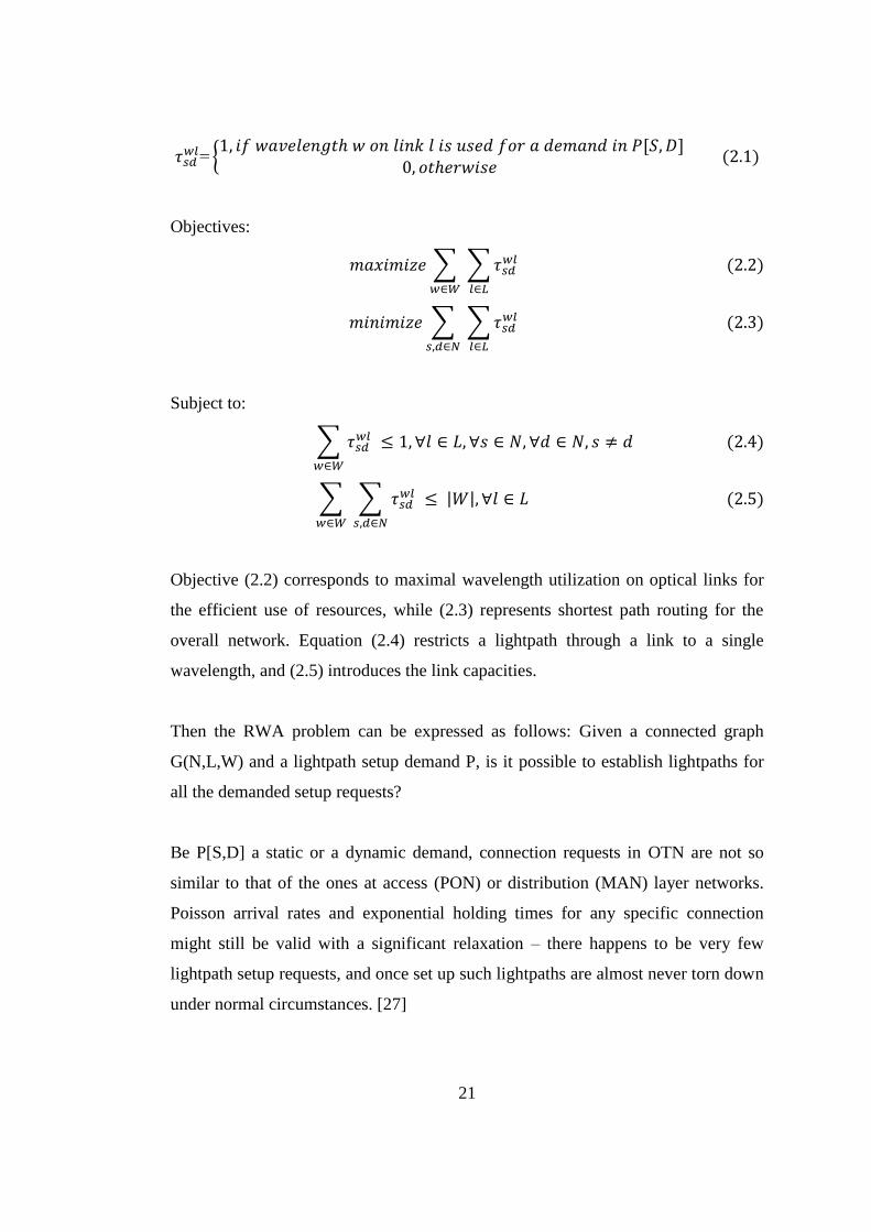
Objectives:

∑ ∑

∑ ∑

Subject to:

∑

∑ ∑

| |

Objective (2.2) corresponds to maximal wavelength utilization on optical links for

the efficient use of resources, while (2.3) represents shortest path routing for the

overall network. Equation (2.4) restricts a lightpath through a link to a single

wavelength, and (2.5) introduces the link capacities.

Then the RWA problem can be expressed as follows: Given a connected graph

G(N,L,W) and a lightpath setup demand P, is it possible to establish lightpaths for

all the demanded setup requests?

Be P[S,D] a static or a dynamic demand, connection requests in OTN are not so

similar to that of the ones at access (PON) or distribution (MAN) layer networks.

Poisson arrival rates and exponential holding times for any specific connection

might still be valid with a significant relaxation – there happens to be very few

lightpath setup requests, and once set up such lightpaths are almost never torn down

under normal circumstances. [27]

22

What is more, each lightpath has to be protected against failures. Since such

lightpaths in the optical core are used to transmit traffic related to thousands (if not

millions) of second level customers (customers’ customers), any service outage has

very dramatic effects. While 99.97% availability (~ 3 minutes of downtime per

week) might be enough for ordinary accounts [28], even six nines (99.9999% ~ 31.5

seconds of downtime per year) may be unacceptable for some highly critical core

layer ISP accounts [14]. Therefore, RWA problem has to be solved in conjunction

with the protection switching scenarios, so as to provide highest levels of resilience

and availability in OTN.

23

CHAPTER 3

PROTECTION SWITCHING IN OTN

Since optical cross connects (OXCs) and DWDM links, which do lie at the very

heart of international/intercontinental OTN, are responsible for delivery of the most

critical amount of traffic, proper route restoration mechanisms have to be deployed

to recover from any link and/or node failure. Main objective of recovery techniques

that are employed in any network architecture should be to autonomously, rapidly,

adaptively, and without great additional cost in terms of redundant capacity reroute

the affected traffic, so as to minimize the information lost during outages.

Taking into consideration that simultaneous multiple failures occur very

infrequently, major interest in literature is on recovery from a single link and/or

node failure. Especially for dense mesh topologies, it is enough safe to assume that

the next failure will likely to happen after all the previously affected traffic

(lightpaths) has been restored. With such an assumption, amount of redundant

capacity required to design a self-protecting network is significantly reduced.

In typical WAN, route restoration is a functionality offered at Layer-3. Whenever a

timer expires or an alarm is triggered routing process is invoked and new routes are

computed. Depending on the routing algorithm used and the complexity of network

topology convergence time may increase up to the order of minutes. However due

to the above-mentioned SLA reasons, in optical domain much tighter timing targets

have to be set for fast lightpath recovery. Because in case recovery cannot be

accomplished in a short period of time, upper layer route restoration mechanisms

take place. [29]

24

Protection switching is the set of tools and algorithms developed to replace any

failed network resource with a pre-assigned backup. Pre-assignment, which

constitutes the basic distinction from route restoration, avoids additional lightpath

setup/teardown events at intermediate nodes. As described in [30], protection

switching approaches should;

Run in a scalable manner to be able to recover numerous lightpath services

concurrently,

Be independent from upper layer protocols to support any client type (such

as SDH, ATM, GbE, FC, etc.),

Utilize a robust signaling methodology to circumvent any additional

failures, and

Not rely on non-time-critical functions (for example, fault localization

should not be a part of protection switching) for the most immediate

behavior.

After an extensive research and development, generic protection switching tools

and methodologies are more or less standardized for linear trails [31], ring

topologies [32], and mesh networks [33]. However due to the multi-dimensional

heterogeneity of transport networks and commercial ISP business practices, there is

still much to do for mesh optical core networks. Appendix A lists the principle

objectives of further investigations.

There are several metrics that may be used to evaluate the performance of a

protection switching technique/algorithm. Among these; recovery success ratio and

speed of recovery are the most vital ones, which do bother the OTN clients.

Capacity efficiency and implementation complexity are the two metrics, which refer

mostly to the operational costs of ISPs. The number of signaling messages

exchanged is already outdated with the out-of-band OOS in OTN encapsulation

hierarchy presented in 2.1.2. In the following sections we introduce the taxonomy

of protection switching in optical networks with a major focus on recovery success

ratio, speed of recovery, and resource efficiency.

25

3.1. Computational Concerns

Two questions to be addressed for evaluating protection switching computation

techniques in optical networks are;

I. When and in how much time backup lightpaths are assigned?

II. How backup lightpaths are computed and the decision is coordinated?

Answers to the first question can be either before failure happens, or right after any

link/node failure. Considering the fact that protection switching has to take place as

soon as possible, preplanned lightpath creation seems to be the best choice. In

literature the other approach is even called route restoration rather than protection

switching. [30, 34]

To catch up with the route restoration timers, switching from (originally working)

failed lightpath to (associated backup) protection lightpath has to complete in the

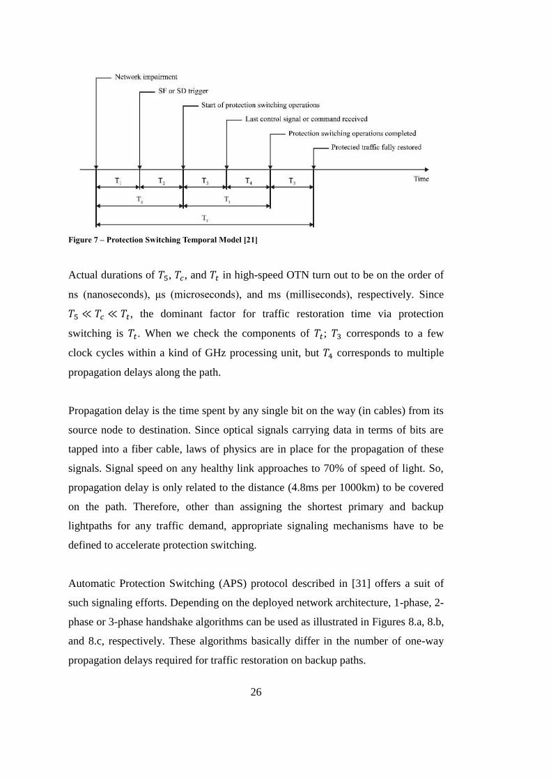
order of tens of milliseconds. Temporal model of protection switching given in

Figure 7 identifies the following happenings within that time; [31]

𝑇1: Network impairment should be detected either through sophisticated

alarm indicators, or simply via Signal Failure/Degradation (SF/SD),

𝑇2: Hold-off time (sometimes referred to as waiting time) should pass to

make sure that it was not a false alarm,

𝑇3: Protection path to be switched on to should be selected,

𝑇4: Decision should be propagated to both communicating end nodes,

𝑇5: Recovery time should elapse for data link frames to be synchronized.

Confirmation (protection switching is required) Time: 𝑇𝑐 = 𝑇1 + 𝑇2

Transfer (protection switching is carried out) Time: 𝑇𝑡 = 𝑇3 + 𝑇4

Traffic Restoration (lightpath services are up and running again) Time:

𝑇𝑟 = 𝑇1 + 𝑇2 + 𝑇3 + 𝑇4 + 𝑇5 = 𝑇𝑐 + 𝑇𝑡 + 𝑇5

26

Figure 7 – Protection Switching Temporal Model [21]

Actual durations of 𝑇5, 𝑇𝑐, and 𝑇𝑡 in high-speed OTN turn out to be on the order of

ns (nanoseconds), μs (microseconds), and ms (milliseconds), respectively. Since

𝑇5 𝑇𝑐 𝑇𝑡, the dominant factor for traffic restoration time via protection

switching is 𝑇𝑡. When we check the components of 𝑇𝑡; 𝑇3 corresponds to a few

clock cycles within a kind of GHz processing unit, but 𝑇4 corresponds to multiple

propagation delays along the path.

Propagation delay is the time spent by any single bit on the way (in cables) from its

source node to destination. Since optical signals carrying data in terms of bits are

tapped into a fiber cable, laws of physics are in place for the propagation of these

signals. Signal speed on any healthy link approaches to 70% of speed of light. So,

propagation delay is only related to the distance (4.8ms per 1000km) to be covered

on the path. Therefore, other than assigning the shortest primary and backup

lightpaths for any traffic demand, appropriate signaling mechanisms have to be

defined to accelerate protection switching.

Automatic Protection Switching (APS) protocol described in [31] offers a suit of

such signaling efforts. Depending on the deployed network architecture, 1-phase, 2-

phase or 3-phase handshake algorithms can be used as illustrated in Figures 8.a, 8.b,

and 8.c, respectively. These algorithms basically differ in the number of one-way

propagation delays required for traffic restoration on backup paths.

27

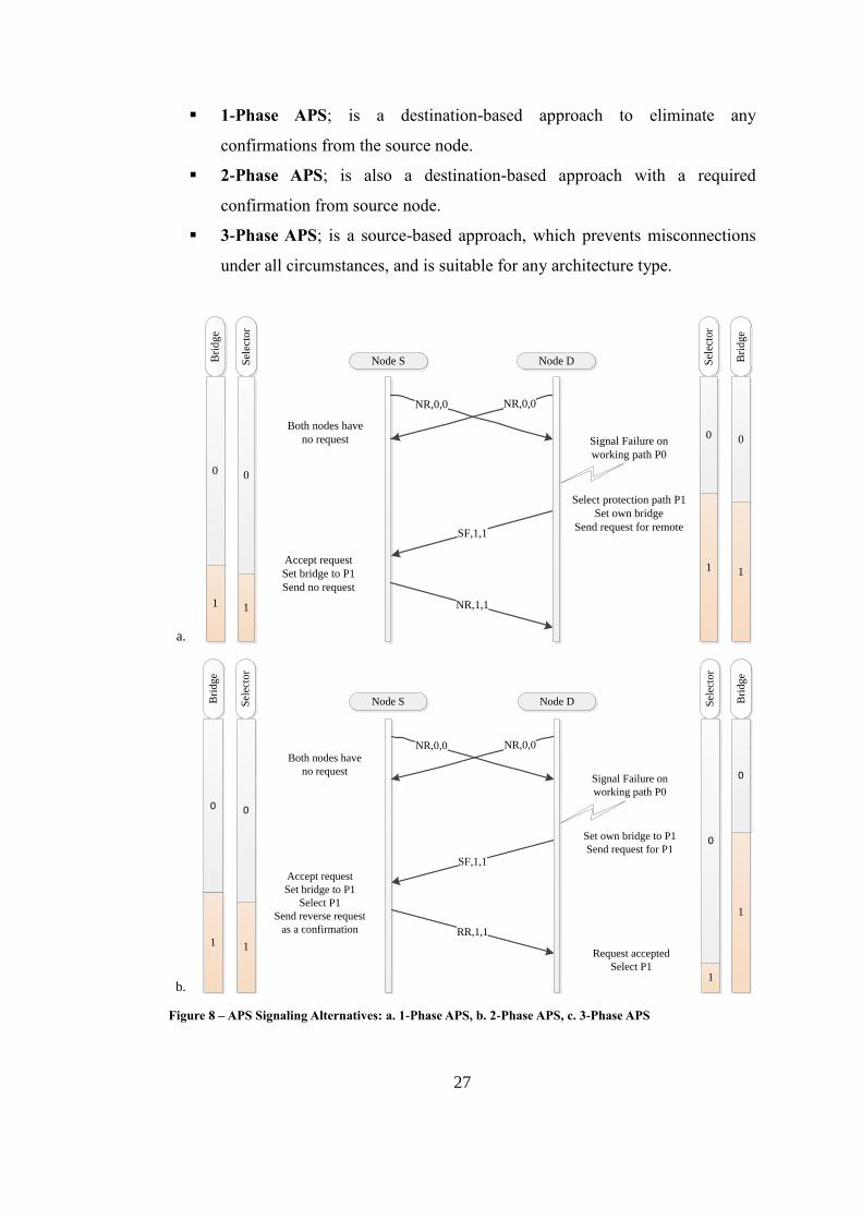
1-Phase APS; is a destination-based approach to eliminate any

confirmations from the source node.

2-Phase APS; is also a destination-based approach with a required

confirmation from source node.

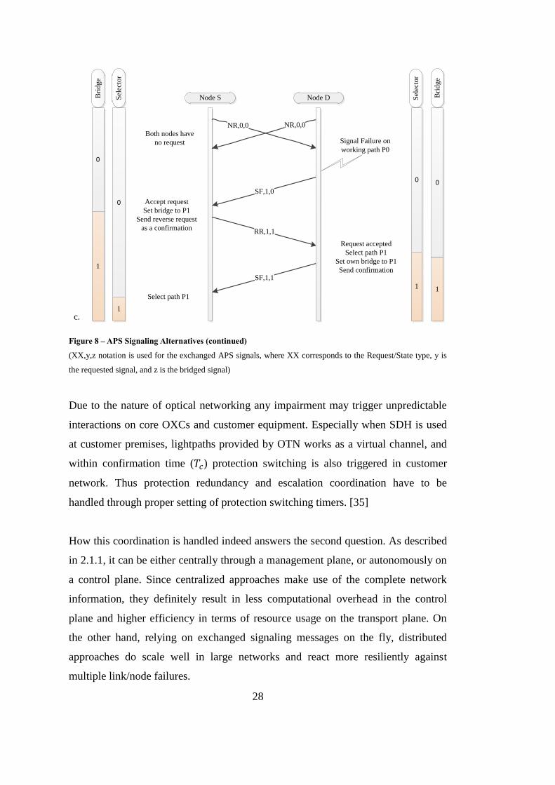
3-Phase APS; is a source-based approach, which prevents misconnections

under all circumstances, and is suitable for any architecture type.

Node S Node D

NR,0,0NR,0,0

Sel

ecto

r

Bri

dge

Bri

dge

Sel

ecto

r

Both nodes have

no request

Select protection path P1

Set own bridge

Send request for remote

Accept request

Set bridge to P1

Send no request

Signal Failure on

working path P0

NR,1,1

SF,1,1

00

0 0

a.

1 1

1 1

Bri

dg

e

0

Node S Node D

NR,0,0NR,0,0

Sel

ecto

r

Bri

dg

e

Sel

ecto

r

Both nodes have

no request

Set own bridge to P1

Send request for P1

Accept request

Set bridge to P1

Select P1

Send reverse request

as a confirmation

Signal Failure on

working path P0

RR,1,1

SF,1,1

00

0

Request accepted

Select P1

b.

1 1

1

1

Figure 8 – APS Signaling Alternatives: a. 1-Phase APS, b. 2-Phase APS, c. 3-Phase APS

28

Node S Node D

NR,0,0NR,0,0S

elec

tor

Bri

dge

Bri

dge

Sel

ecto

r

Both nodes have

no request

Select path P1

Accept request

Set bridge to P1

Send reverse request

as a confirmation

Signal Failure on

working path P0

RR,1,1

SF,1,0

0

0

0 0

Request accepted

Select path P1

Set own bridge to P1

Send confirmationSF,1,1

c.

1 1

1

1

Figure 8 – APS Signaling Alternatives (continued)

(XX,y,z notation is used for the exchanged APS signals, where XX corresponds to the Request/State type, y is

the requested signal, and z is the bridged signal)

Due to the nature of optical networking any impairment may trigger unpredictable

interactions on core OXCs and customer equipment. Especially when SDH is used

at customer premises, lightpaths provided by OTN works as a virtual channel, and

within confirmation time (𝑇𝑐) protection switching is also triggered in customer

network. Thus protection redundancy and escalation coordination have to be

handled through proper setting of protection switching timers. [35]

How this coordination is handled indeed answers the second question. As described

in 2.1.1, it can be either centrally through a management plane, or autonomously on

a control plane. Since centralized approaches make use of the complete network

information, they definitely result in less computational overhead in the control

plane and higher efficiency in terms of resource usage on the transport plane. On

the other hand, relying on exchanged signaling messages on the fly, distributed

approaches do scale well in large networks and react more resiliently against

multiple link/node failures.

29

Nevertheless, centralized control might not be that possible within the multi-domain

nature of real carriers. Limited (better to say summarized) information is available

on border nodes, and inter-domain links cannot guarantee to provide backup

lightpaths for all neighboring carriers [36]. Therefore, a broad set of network

topologies have to run distributed and/or hierarchical protection switching

algorithms by forming trust relationships and securely sharing any required

monitoring or billing information via peering mechanisms [37].

3.2. Resource Efficiency

The more a network is utilized the more efficient turns out to be the investment

made. While trying to provide the best protection switching performance in terms of

time, we cannot underestimate the cost of laying new optical cables or installing

more active devices. Therefore, equilibrium has to be reached between network

redundancy and efficiency. Computation of primary and backup lightpaths has to be

carried out in a manner to optimize resource utilization via sharing as many links as

possible. APS architectures in point-to-point systems could be a nice starter to

define the levels of efficiency in optical networks: [30, 38]

(1+1) Protection: In this approach, practically, there are two working

lightpaths. Transmitter-receiver pairs on both sides of a communication

channel select among the two incoming signals on a quality basis. And there

is no need for any signaling overhead in case of a failure. However, the

required split up at the transmitter result in 3dB optical signal loss.

(1:1) Protection: In this approach, there is one pre-computed backup path

(DBPP – Dedicated Backup Path Protection) for each working lightpath.

Advantage against (1+1) protection is backup paths can be utilized with

low-priority traffic when associated working lightpaths are functional. But

in case of failures, a low signaling overhead (either 1-phase or 2-phase APS)

takes place. And depending on the defined priorities, suspended traffic is

switched on to the backup path.

30

(M:N) Protection: This approach is an extension and generalization of (1:1)

protection. The only difference is there are M backup paths for N working

lightpaths. Since N is typically greater than M, resources are shared (SBPP –

Shared Backup Path Protection) with improved efficiency. Obviously,

signaling overhead in case of a failure is expected to be higher (3-phase

APS) for this implementation. For the most optimistic scenarios it may be

possible for a lightpath to survive even after up to M link faults, but when

failures effect all N working lightpaths only M of them can survive in this

scheme.

With proper sharing in a mesh network, protection capacity may be well below 60%

of the working capacity [39]. Though a value-based approach on service provider

reliability costs (capital investments and operational expenses) and beneficial

savings (reduced revenue loss and decreased SLA penalties) in [28] has shown that

shared mesh network design posts an 8% saving over the dedicated protection.

One of the main issues while trying to increase efficiency is to deal with the Shared

Risk Groups (SRG). Risk groups can be defined as a set = { | | | },

where is a set of links (Shared Risk Link Group (SRLG)) and nodes (Shared Risk

Node Group (SRNG)), or both. Given any two network elements and , if there

exists no any SRG , such that both and , then and are said to

be SRG-independent. Given a path = { 1 1 12 2 1 } and a

network element , if there exists no any SRG , such that both and either

or , then and are said to be SRG-independent. Given a pair of

paths 1 and 2, if each link and each node in 1 is SRG-independent with 2 and

vice versa, then 1 and 2 are said to be SRG-disjoint.

SRG is an important network design parameter especially when assigning

protection lightpaths. Nevertheless, construction and deployment of optical cables

introduce additional complexities, which can only be dealt with by human

interaction. As described in [3] there may be tens of fiber cores within an optical

cable. Lightpaths (i.e. wavelengths) on a fiber core can be distinguished on a node,

31

to which that specific core is connected. But there are no any means to understand

whether fibers connected to different ports of an active device are assembled in the

same ribbon with each other, or not. So, deployment procedures for optical cables

underground not only have to follow the technical guidelines, but also obey

standard documentation principles.

Fiber cables in optical transport systems are buried in a sequence of right of way

(ROW) structures, which are frequently obtained from railway or pipeline

companies. The economics of such ROW leasing in long-haul runs often

necessitates several carriers share the costs. However, this collaboration may turn

out to be a kind of fate sharing as well, since numerous carrier cables lay in close

proximity to each other. What is worse, physical layout of the network may nullify

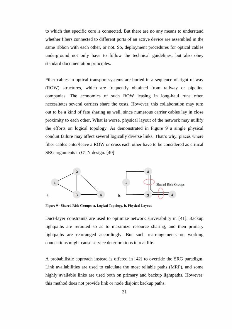
the efforts on logical topology. As demonstrated in Figure 9 a single physical

conduit failure may affect several logically diverse links. That’s why, places where

fiber cables enter/leave a ROW or cross each other have to be considered as critical

SRG arguments in OTN design. [40]

Figure 9 - Shared Risk Groups: a. Logical Topology, b. Physical Layout

Duct-layer constraints are used to optimize network survivability in [41]. Backup

lightpaths are rerouted so as to maximize resource sharing, and then primary

lightpaths are rearranged accordingly. But such rearrangements on working

connections might cause service deteriorations in real life.

A probabilistic approach instead is offered in [42] to override the SRG paradigm.

Link availabilities are used to calculate the most reliable paths (MRP), and some

highly available links are used both on primary and backup lightpaths. However,

this method does not provide link or node disjoint backup paths.

32

Two aspects have to be considered while trying to improve efficiency in OTN:

I. Load Balancing: Computing primary and backup lightpaths as diverse as

possible would utilize most of the network resources in a homogenous

fashion, and leave available wavelengths for further traffic demand.

II. Shared Risk Groups: Applying (M:N) protection techniques (SBPP) for

those primary lightpaths that do not have any SRG would avoid contention

in case of a failure, and reduce the blocking probability.

3.3. Topological Facts

There are two dimensions of topological discussions in lightpath protection:

I. Diversity of the primary and backup paths

II. Overall topology of the network

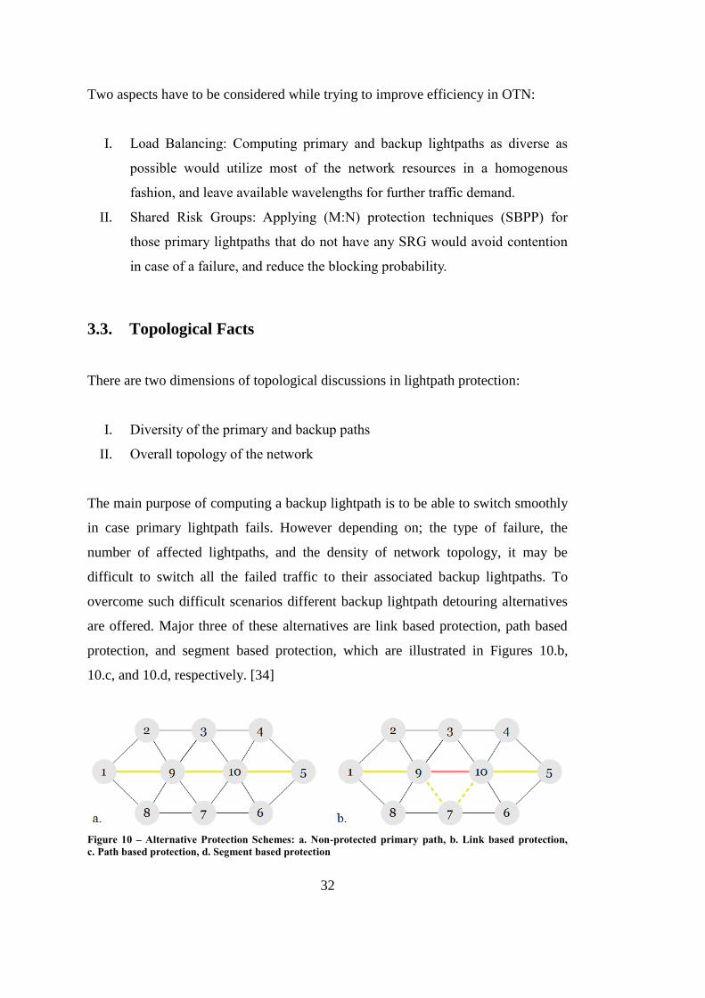
The main purpose of computing a backup lightpath is to be able to switch smoothly

in case primary lightpath fails. However depending on; the type of failure, the

number of affected lightpaths, and the density of network topology, it may be

difficult to switch all the failed traffic to their associated backup lightpaths. To

overcome such difficult scenarios different backup lightpath detouring alternatives

are offered. Major three of these alternatives are link based protection, path based

protection, and segment based protection, which are illustrated in Figures 10.b,

10.c, and 10.d, respectively. [34]

Figure 10 – Alternative Protection Schemes: a. Non-protected primary path, b. Link based protection,

c. Path based protection, d. Segment based protection

33

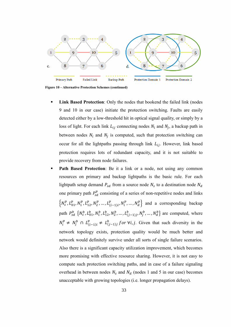
Figure 10 – Alternative Protection Schemes (continued)

Link Based Protection: Only the nodes that bookend the failed link (nodes

9 and 10 in our case) initiate the protection switching. Faults are easily

detected either by a low-threshold hit in optical signal quality, or simply by a

loss of light. For each link connecting nodes and , a backup path in

between nodes and is computed, such that protection switching can

occur for all the lightpaths passing through link . However, link based

protection requires lots of redundant capacity, and it is not suitable to

provide recovery from node failures.

Path Based Protection: Be it a link or a node, not using any common

resources on primary and backup lightpaths is the basic rule. For each

lightpath setup demand from a source node to a destination node

one primary path 𝑝 consisting of a series of non-repetitive nodes and links

{ 𝑝 1

𝑝 1𝑝 12

𝑝 2𝑝 1

𝑝 𝑝

𝑝} and a corresponding backup

path 𝑏 {

𝑏 1𝑏 1

𝑏 12𝑏 2

𝑏 1 𝑏

𝑏 𝑏} are computed, where

𝑝

𝑏 ∩ 1 𝑝 1

𝑏 𝑗. Given that such diversity in the

network topology exists, protection quality would be much better and

network would definitely survive under all sorts of single failure scenarios.

Also there is a significant capacity utilization improvement, which becomes

more promising with effective resource sharing. However, it is not easy to

compute such protection switching paths, and in case of a failure signaling

overhead in between nodes and (nodes 1 and 5 in our case) becomes

unacceptable with growing topologies (i.e. longer propagation delays).

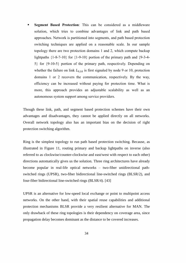
34

Segment Based Protection: This can be considered as a middleware

solution, which tries to combine advantages of link and path based

approaches. Network is partitioned into segments, and path based protection

switching techniques are applied on a reasonable scale. In our sample

topology there are two protection domains 1 and 2, which compute backup

lightpaths {1-8-7-10} for {1-9-10} portion of the primary path and {9-3-4-

5} for {9-10-5} portion of the primary path, respectively. Depending on

whether the failure on link 9 1 is first signaled by node 9 or 10, protection

domains 1 or 2 recovers the communication, respectively. By the way,

efficiency can be increased without paying for protection time. What is

more, this approach provides an adjustable scalability as well as an

autonomous system support among service providers.

Though these link, path, and segment based protection schemes have their own

advantages and disadvantages, they cannot be applied directly on all networks.

Overall network topology also has an important bias on the decision of right

protection switching algorithm.

Ring is the simplest topology to run path based protection switching. Because, as

illustrated in Figure 11, routing primary and backup lightpaths on inverse (also

referred to as clockwise/counter-clockwise and east/west with respect to each other)

directions automatically gives us the solution. Three ring architectures have already

become popular in real-life optical networks – two-fiber unidirectional path-

switched rings (UPSR), two-fiber bidirectional line-switched rings (BLSR/2), and

four-fiber bidirectional line-switched rings (BLSR/4). [43]

UPSR is an alternative for low-speed local exchange or point to multipoint access

networks. On the other hand, with their spatial reuse capabilities and additional

protection mechanisms BLSR provide a very resilient alternative for MAN. The

only drawback of these ring topologies is their dependency on coverage area, since

propagation delay becomes dominant as the distance to be covered increases.

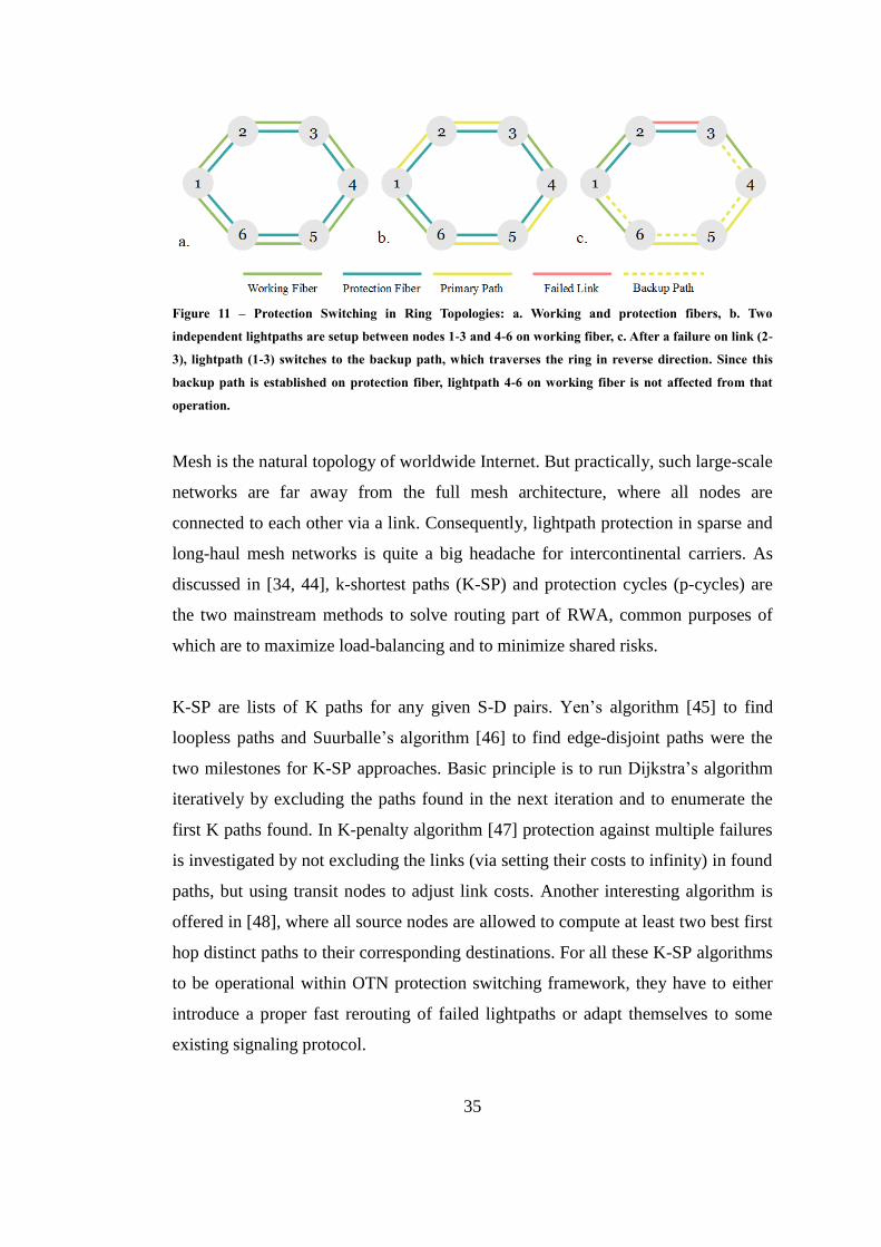
35

Figure 11 – Protection Switching in Ring Topologies: a. Working and protection fibers, b. Two

independent lightpaths are setup between nodes 1-3 and 4-6 on working fiber, c. After a failure on link (2-

3), lightpath (1-3) switches to the backup path, which traverses the ring in reverse direction. Since this

backup path is established on protection fiber, lightpath 4-6 on working fiber is not affected from that

operation.

Mesh is the natural topology of worldwide Internet. But practically, such large-scale

networks are far away from the full mesh architecture, where all nodes are

connected to each other via a link. Consequently, lightpath protection in sparse and

long-haul mesh networks is quite a big headache for intercontinental carriers. As

discussed in [34, 44], k-shortest paths (K-SP) and protection cycles (p-cycles) are

the two mainstream methods to solve routing part of RWA, common purposes of

which are to maximize load-balancing and to minimize shared risks.

K-SP are lists of K paths for any given S-D pairs. Yen’s algorithm [45] to find

loopless paths and Suurballe’s algorithm [46] to find edge-disjoint paths were the

two milestones for K-SP approaches. Basic principle is to run Dijkstra’s algorithm

iteratively by excluding the paths found in the next iteration and to enumerate the

first K paths found. In K-penalty algorithm [47] protection against multiple failures

is investigated by not excluding the links (via setting their costs to infinity) in found

paths, but using transit nodes to adjust link costs. Another interesting algorithm is

offered in [48], where all source nodes are allowed to compute at least two best first

hop distinct paths to their corresponding destinations. For all these K-SP algorithms

to be operational within OTN protection switching framework, they have to either

introduce a proper fast rerouting of failed lightpaths or adapt themselves to some

existing signaling protocol.

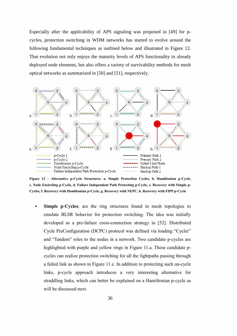
36

Especially after the applicability of APS signaling was proposed in [49] for p-

cycles, protection switching in WDM networks has started to evolve around the

following fundamental techniques as outlined below and illustrated in Figure 12.

That evolution not only enjoys the maturity levels of APS functionality in already

deployed node elements, but also offers a variety of survivability methods for mesh

optical networks as summarized in [50] and [51], respectively.

Figure 12 – Alternative p-Cycle Structures: a. Simple Protection Cycles, b. Hamiltonian p-Cycle,

c. Node Encircling p-Cycle, d. Failure Independent Path Protecting p-Cycle, e. Recovery with Simple p-

Cycles, f. Recovery with Hamiltonian p-Cycle, g. Recovery with NEPC, h. Recovery with FIPP p-Cycle

Simple p-Cycles; are the ring structures found in mesh topologies to

emulate BLSR behavior for protection switching. The idea was initially

developed as a pre-failure cross-connection strategy in [52]. Distributed

Cycle PreConfiguration (DCPC) protocol was defined via loading “Cycler”

and “Tandem” roles to the nodes in a network. Two candidate p-cycles are

highlighted with purple and yellow rings in Figure 11.a. These candidate p-

cycles can realize protection switching for all the lightpaths passing through

a failed link as shown in Figure 11.e. In addition to protecting such on-cycle

links, p-cycle approach introduces a very interesting alternative for

straddling links, which can better be explained on a Hamiltonian p-cycle as

will be discussed next.

37

Hamiltonian p-Cycle (introduced as Hamiltonian Cycle Protection in [53]);

is the longest possible p-cycle for a network, since it traverses all the nodes

once. What is more, all links in a network topology can be protected with a

single Hamiltonian p-cycle, because any link would be either an on-cycle

link, or a straddling link. Any link (edge), whose end-points are connected to

nodes (vertices) on a p-cycle, but the link itself is not a part of the p-cycle, is

called a straddling link. Existence (link (5-6)) and two diversely routed

protection path alternatives (paths {5-1-2-6} and {5-4-3-6}) of such

straddling links are illustrated in Figures 11.b and 11.f, respectively. Though

Hamiltonian cycles do not exist for all topologies, this can and should be

mitigated by service providers as a network design issue. Other than acting

as an option for protection switching, presence of a Hamiltonian cycle

makes resolution of graph coloring problem for spectrum allocation much

simpler, since the auxiliary graph would have only two nodes.

Node Encircling p-Cycle (NEPC); is developed to protect the traffic

passing through a particular node in [54]. Since there are no any means to

deal with the originated or terminated lightpaths on that specific node, only

the transit lightpaths are of concern. Beautiful thing is; each failed node

emulates a straddling link for all passing by lightpaths, so that two distinct

backup paths can be found on the p-cycle as illustrated in Figure 11.g. But it

is not always possible to allocate as simple p-cycles (i.e. traversing links and

nodes just once) as given in Figure 11.c to encircle each node. When it

comes to finding and configuring non-simple p-cycles, computation

complexity increases and management flexibility diminishes.

Failure Independent Path Protection (FIPP) p-Cycles; are structures for

defining compatible route sets to share the pre-cross-connected protection

resources. Figures 11.d and 11.h demonstrate how such a FIPP p-cycle can

be formed for 2 mutually disjoint paths and how lightpaths can be recovered

independent of the failure (i.e. node or link), respectively. Nevertheless,

since enumeration of compatible route groups for a given demand has

combinatorial complexity, a reverse engineering solution for a candidate

FIPP p-cycle is offered in [55], which is quite not practical in real networks.

38

Though all those projections of ring topologies on mesh networks sound impressive,

their implementation still needs to follow hybrid methodologies. At initial network

setup a central processing might be helpful to compute the most efficient primary

and backup lightpath provisioning. Whenever failures start to occur in runtime, next

backup lightpaths have to be addressed continuously in a distributed manner.

39

CHAPTER 4

PROBLEM DEFINITION AND PROPOSED SOLUTION

In this study we primarily focus on cases, which do replicate the real life

experiences regarding protection switching. Our main aim is to provide a new

protection switching framework in OTN.

We have several assumptions, and based on these assumptions we propose quasi-

ring decomposition for mesh networks. We call our approach TZAR – Time Zone

based Approximation to Ring. Currently we assume APS signaling described in 3.1

is used, however we believe that it is also possible to use GMPLS control plane.

4.1. Assumptions

I. If the maximum ring length can be relaxed from 1200 km (~6 ms

propagation delay) to 48000 km (~240 ms propagation delay), then resulting

worst-case service restoration time target can also be relaxed from 60 ms (up

to 10 ms for failure detection and 50 ms for switch time) to the order of 300

ms. Four justifications for the possibility of that relaxation are:

a. “Switch time” network objective has already been applied as 300 ms

for transoceanic Multiplex Section shared protection rings in [56].

This is also applicable to situations, where distances between the

nodes of a ring exceed 1500 km.

b. A “Hold-off timer” of up to 10 seconds in steps of 100 ms is suggested

across cascaded Ethernet linear protection switching groups to give

chance for an upstream ring to fix the encountered problem. [57]

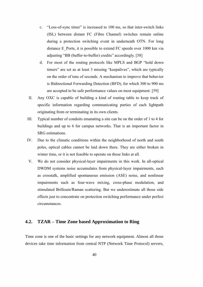
40

c. “Loss-of-sync timer” is increased to 100 ms, so that inter-switch links

(ISL) between distant FC (Fibre Channel) switches remain online

during a protection switching event in underneath OTN. For long

distance E_Ports, it is possible to extend FC speeds over 1000 km via

adjusting “BB (buffer-to-buffer) credits” accordingly. [58]

d. For most of the routing protocols like MPLS and BGP “hold down

timers” are set as at least 3 missing “keepalives”, which are typically

on the order of tens of seconds. A mechanism to improve that behavior

is Bidirectional Forwarding Detection (BFD), for which 300 to 900 ms

are accepted to be safe performance values on most equipment. [59]

II. Any OXC is capable of building a kind of routing table to keep track of

specific information regarding communicating parties of each lightpath

originating from or terminating in its own clients.

III. Typical number of conduits emanating a site can be on the order of 1 to 4 for

buildings and up to 6 for campus networks. That is an important factor in

SRG estimations.

IV. Due to the climatic conditions within the neighborhood of north and south

poles, optical cables cannot be laid down there. They are either broken in

winter time, or it is not feasible to operate on those links at all.

V. We do not consider physical-layer impairments in this work. In all-optical

DWDM systems noise accumulates from physical-layer impairments, such

as crosstalk, amplified spontaneous emission (ASE) noise, and nonlinear

impairments such as four-wave mixing, cross-phase modulation, and

stimulated Brillouin/Raman scattering. But we underestimate all those side

effects just to concentrate on protection switching performance under perfect

circumstances.

4.2. TZAR – Time Zone based Approximation to Ring

Time zone is one of the basic settings for any network equipment. Almost all those

devices take time information from central NTP (Network Time Protocol) servers,

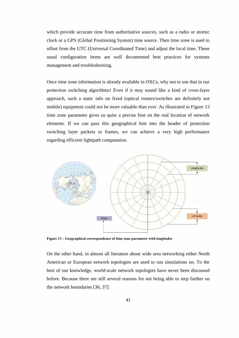
41

which provide accurate time from authoritative sources, such as a radio or atomic

clock or a GPS (Global Positioning System) time source. Then time zone is used to

offset from the UTC (Universal Coordinated Time) and adjust the local time. These

usual configuration items are well documented best practices for systems

management and troubleshooting.

Once time zone information is already available in OXCs, why not to use that in our

protection switching algorithms! Even if it may sound like a kind of cross-layer

approach, such a static info on fixed (optical routers/switches are definitely not

mobile) equipment could not be more valuable than ever. As illustrated in Figure 13

time zone parameter gives us quite a precise hint on the real location of network

elements. If we can pass this geographical hint into the header of protection

switching layer packets or frames, we can achieve a very high performance

regarding efficient lightpath computation.

Figure 13 – Geographical correspondence of time zone parameter with longitudes

On the other hand, in almost all literature about wide area networking either North

American or European network topologies are used to run simulations on. To the

best of our knowledge, world-scale network topologies have never been discussed

before. Because there are still several reasons for not being able to step further on

the network boundaries [36, 37]:

42

Governmental bodies enforce legal control on the cables laid underground.

So, it is not possible for any ISP to install its own optical cables in all

countries.

Spatial distribution of customer base economically restricts any ISP to

operate in a limited geographical coverage and number of POPs (Point Of

Presence).

When it comes to cooperation among neighboring ISPs, following facts

introduce additional complexity on multiple management domains: [60]

▫ Implementation differences in heterogeneous active network elements

▫ Administrative restrictions on sharing topology and route information

▫ Suboptimal SLA policies, which cause reluctance at the earning side

However, we believe that globalization trends in ICT industry are about to hit the

OTN. Emerging business justifications to support this belief are two-fold:

i. Internet Exchange Points: Starting with Finland and Norway (probably our

Assumption IV made it necessary) in 1993, Internet Exchange Points (IXP)

are being established around the world to provide service providers a means

to exchange Internet traffic. Colocation at an IXP not only gives relevant

ISPs an opportunity to reach each other in a fast and cheap manner, but also

results in a high-bandwidth and low-latency performance for the exchanged

traffic. [61]

Internet traffic is exchanged through Border Gateway Protocol (BGP), in

which all communicating networks are represented with corresponding

Autonomous System (AS) numbers. Routes among different AS are

announced through peering links on a policy basis. Since there is an

abundance of ISPs within most of IXP sites, it is a strategic decision of each

AS to select with whom to peer. But as discussed in [62] rather immediate

traffic recovery from emergency situations can be accomplished just inside

the IXPs. Figure 14 lay out the physical (solid lines) and logical (dashed

peering links) topologies relating IXP and AS domains.

43

IXP A

Internet Exchange Points

Autonomous Systems Domain

IXP B

IXP C

AS 4AS 5

AS 1

AS 2

AS 3

AS 2

AS 3AS 1

Figure 14 – Autonomous Systems peering at Internet Exchange Points

Leading IXPs, such as the ones located in Frankfurt (DE-CIX), Amsterdam

(AMS-IX), and London (LINX) have already made 100Gbps ports available

on their switching fabrics and passed the Tbps throughput thresholds [63].

But the most exciting business strategy is developed by Equinix, which

operates as a network of IXPs around the globe (having presence in Paris,

New York, Tokyo, Sydney, etc.). Any two AS on distant IXPs may soon peer

via Ethernet over DWDM tunneling.

ii. Content Delivery Networks: Cloud computing era is driven by large

software companies, which launch their products on Software as a Service

(SaaS) platforms, such as Microsoft Azure and Amazon CloudFront.

Targeting to provide the best performance and to excel in the user

experience, those platforms started to reside on Content Delivery Networks

(CDN), which are distributed data centers across the Internet.

CDN nodes are either operated individually, or collocated on an ISP site. In

any case the interconnectivity (dashed links) is provided preferentially by

dark fibers (solid lines) leased from two or more Tier-1 ISPs as shown in

Figure 15. Many application delivery switching functionalities, such as web

caching for lower latency, encryption for improved security, compression for

efficient bandwidth consumption, and load-balancing for scalability and

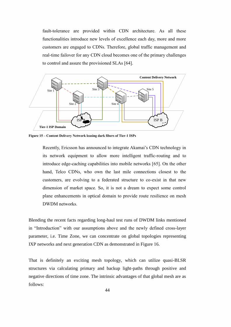
44

fault-tolerance are provided within CDN architecture. As all these

functionalities introduce new levels of excellence each day, more and more

customers are engaged to CDNs. Therefore, global traffic management and

real-time failover for any CDN cloud becomes one of the primary challenges

to control and assure the provisioned SLAs [64].

ISP BISP A

Site 2

Site 1 Site 3 Site 5

Content Delivery Network

Tier-1 ISP Domain

Site 4

Figure 15 – Content Delivery Network leasing dark fibers of Tier-1 ISPs

Recently, Ericsson has announced to integrate Akamai’s CDN technology in

its network equipment to allow more intelligent traffic-routing and to

introduce edge-caching capabilities into mobile networks [65]. On the other

hand, Telco CDNs, who own the last mile connections closest to the

customers, are evolving to a federated structure to co-exist in that new

dimension of market space. So, it is not a dream to expect some control

plane enhancements in optical domain to provide route resilience on mesh

DWDM networks.

Blending the recent facts regarding long-haul test runs of DWDM links mentioned

in “Introduction” with our assumptions above and the newly defined cross-layer

parameter, i.e. Time Zone, we can concentrate on global topologies representing

IXP networks and next generation CDN as demonstrated in Figure 16.

That is definitely an exciting mesh topology, which can utilize quasi-BLSR

structures via calculating primary and backup light-paths through positive and

negative directions of time zone. The intrinsic advantages of that global mesh are as

follows:

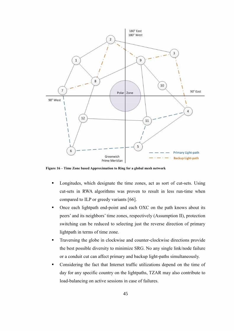
45

Figure 16 – Time Zone based Approximation to Ring for a global mesh network

Longitudes, which designate the time zones, act as sort of cut-sets. Using

cut-sets in RWA algorithms was proven to result in less run-time when

compared to ILP or greedy variants [66].

Once each lightpath end-point and each OXC on the path knows about its

peers’ and its neighbors’ time zones, respectively (Assumption II), protection

switching can be reduced to selecting just the reverse direction of primary

lightpath in terms of time zone.

Traversing the globe in clockwise and counter-clockwise directions provide

the best possible diversity to minimize SRG. No any single link/node failure

or a conduit cut can affect primary and backup light-paths simultaneously.

Considering the fact that Internet traffic utilizations depend on the time of

day for any specific country on the lightpaths, TZAR may also contribute to

load-balancing on active sessions in case of failures.

46

The utmost performance is expected for any S-D pair located 135° to 225°

apart from each other. When the magnitude of time zone difference is 12 ∓3

hours, setting up the backup light-path in reverse direction makes the most

sense.

4.3. Heuristics

We introduce our heuristics making an analogy from Ad-hoc On-demand Distance

Vector (AODV) routing [67] offered for Mobile Ad-hoc Networks (MANET), so

that large instances of TZAR can be solved with minimal computational overhead.

Table 6 gives a summary of how we relate AODV with backup lightpath creation in

TZAR.

Table 6 – Relation of AODV with TZAR

AODV TZAR

Path Setup Initiator Route Request (RREQ)

Route Error (RERR)

Signal Fail (SF)

Signal Degrade (SD)

Confirmation Route Reply (RREP) Reverse Request (RR)

Working Path Identifier Sequence Number Connection ID

Distance Identifier Hop Count Time Zone (TZ)

Topology Controller

NET_DIAMETER is used to

control maximum number of

hops between any S-D pair

TZ_DIFFERENCE is used to

control propagation of SD/SF

messages along the path

Timing Controllers PATH_DISCOVERY_TIME

NET_TRAVERSAL_TIME

Hold-off Timers

Wait-to-Restore (WTR)

Message Propagation Broadcast / Unicast Many_Cast / Unicast

Based on that analogy, APS signaling mechanism introduced in section 3.1 is

modified as illustrated in Figure 17. By the way, intermediate nodes are also

participating in our protection switching algorithm via making a kind of 1-phase

handshake on ingress ports and 2-phase handshake on egress ports.

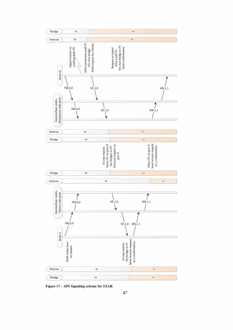
47

Node

SN

ode

D

NR,0,0

NR,0,0

Selector

Bridge

Bridge

Selector

Both

nodes

hav

e

no r

eques

tS

ignal

Fai

lure

on

work

ing p

ath P

0

SF,1,0

0

0

Req

ues

t ac

cepte

d

Sel

ect

pat

h P

1

Set

ow

n b

ridge

to P

1

Sen

d c

onfi

rmat

ion

Bridge

Selector

0

Bridge

Selector 0

0

Inte

rmed

iate

nodes

,

Sourc

e si

de

port

s

Inte

rmed

iate

nodes

,

Des

tinat

ion s

ide

port

s

Sel

ect

pro

tect

ion p

ath P

1

Set

ow

n b

ridge

Sen

d r

eques

t fo

r re

mote

SF,1,0

NR,0,0

NR,0,0

Acc

ept

reques

t

Sel

ect

P1 o

n p

ort

D

Set

bri

dges

to P

1

Forw

ard r

eques

t on

port

S

SF,1,0

SF,1,0

Acc

ept

reques

t

Set

bri

dge

to P

1

Sen

d r

ever

se r

equ

est

as a

co

nfi

rmat

ion

RR,1,1

RR,1,1

RR,1,1

RR,1,1

Sel

ect

P1 o

n p

ort

S

Sen

d r

ever

se r

eques

t

as a

confi

rmat

ion

0

0

0 11

1

11

1

11

Figure 17 – APS Signaling scheme for TZAR

48

Although it is not apparent in Figure 17, we also assume that bridging to multiple

links on each node is possible. As it will be explained in the heuristic below,

forwarding backup lightpath setup requests on multiple non-overlapping links is

expected to reduce blocking probability.

Table 7 – TZAR Heuristics

Protection Switching initiated by a source node

1. While (Max_Try_Count is not reached) Do

2. Set (TTL Minimum (15, Number of Nodes)) and (Many_Cast 0)

3. Send a lightpath setup request (SF) through a local interface, such that;

i. If (Destination_TZ > Source_TZ) then (Neighbor_TZ < Source_TZ)

ii. Else if (Destination_TZ < Source_TZ) then (Neighbor_TZ > Source_TZ)

iii. Else select a random interface other than the one, on which connection was failed

iv. Initialize RWA_Accumulated with source node/link info, and selected wavelength

SF/RR is processed at intermediate nodes

4. If (Destination_Address Own_Address) then go to Step.8

i. Else if (TTL is expired) then drop the SF

ii. Else if (Conn_ID is cached within Hold_SF) then check RWA_Accumulated

iii. Else decrement TTL, and compute new Many_Cast

5. Check Source_TZ to adjust forwarding interface candidates

6. Update RWA_Accumulated in accordance with selected candidate interfaces

7. For Many_Cast times forward SF through altering next-hop interfaces

Response of destination node

8. If (accumulated wavelengths list is empty) then do nothing

i. Else select the accumulated wavelength on received link

ii. Update RWA_Accumulated for RR

9. Bridge to the protection lightpath

10. Send a unicast reverse request (RR) on the new route

11. If (RR is not received within Hold_RR) then drop Conn_ID from cache

i. Else assign wavelength and select the new lightpath

ii. Update RWA_Accumulated for RR

12. Bridge to the protection lightpath

13. Forward RR along the path in reverse direction

14. If (RR is not received within Hold_RR) then increment Max_Try_Count and go to step 2

i. Else assign wavelength, select and bridge on to the new lightpath

15. If (Max_Try_Count is exceeded) then backup lightpath setup request is blocked and

protection switching is failed

49

Heuristics given in Table 7 figure out the additional features embedded in TZAR.

These add-ons provide suboptimal solutions for protection switching in OTN within

reasonable run times for realistic problem instances.

Protection switching starts with a selection in the source node at step 3. Pre-

assignment, which makes us call our algorithm a protection rather than a

restoration, is based on the TZ parameters of destination and neighboring nodes.

Although first attempt is to switch away from the notified failure, that will not result

in a global ring in every case. Steps 3.iii, 5, 6, and 7 inherently give chances for

shorter backup lightpath creation.

Many_Cast functionality avoids contention in the vicinity of a failure, and reduces

blocking probability for long paths. When compared to broadcast nature of AODV

protocol, a dynamic many_cast operation is much more suitable for effective

wavelength allocation in TZAR. Starting with 0, many_cast counter is adjusted up

to 3 on each hop in accordance with the TTL value. Sort of load balancing is also

provided with steps 2, 4.iii, 6and 7 via randomly selecting the forwarding interfaces

among candidates. As a fruitful side effect of this behavior, protection switching

against multiple failures is also provided. How all these heuristics are implemented

will be explained in the next chapter.

A list of correlations between our heuristics and shared mesh network protection

switching requirements (Appendix A) can be emphasized before proceeding with

the modeling framework and simulation results:

Utilization of existing OOS channel for signaling and OTM hierarchy for

encapsulation per se is a solution to provide backward compatibility (A.1),

to co-exist with APS specifications (A.2), to apply on cascaded or nested

deployments (A.3), to communicate protection switching information

(A.10), to fine-tune counter and timeout variables so as to comply with the

network size and traffic demand (A.20), and to support external commands

(A.24).

50

Keeping track of candidate interfaces and featuring Many_Cast operation

allows consideration of multiple links between nodes as a scalability option

(A.16), and well-bounded wavelength resources per link as a constrained

allocation for protection switching (A.19).

Operation beyond inter-domain boundaries (A4) and bidirectional switching

types (A23) are supported by employing carrier and domain independent

Time_Zone parameter as a cross-layer information.

Protection for multiple ingress and egress lightpaths (A.5), independence of

shared resources on communicating end nodes (A.6), status monitoring and

switching triggers (A.7), concurrent or multiple failures (A.25), and

capability to initiate protection switching on either end or both ends (A.26)

by using SF, RR messages on a granular basis on the levels of both lightpath

clients and traversed nodes.

Managed timers like Hold_RR and counters like Max_Try_Count provide

deterministic recovery times (A.11), protocol failure detection (A.12), and

protection switching activity coordination (A.14).

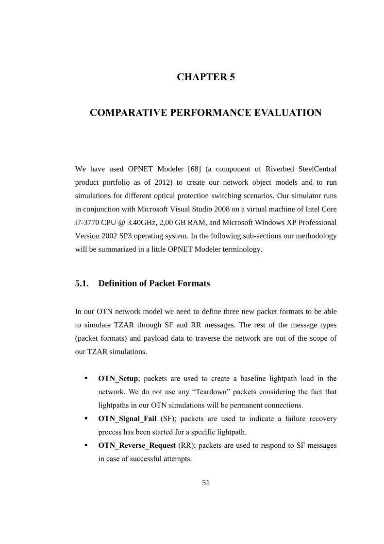
51

CHAPTER 5

COMPARATIVE PERFORMANCE EVALUATION

We have used OPNET Modeler [68] (a component of Riverbed SteelCentral

product portfolio as of 2012) to create our network object models and to run

simulations for different optical protection switching scenarios. Our simulator runs

in conjunction with Microsoft Visual Studio 2008 on a virtual machine of Intel Core

i7-3770 CPU @ 3.40GHz, 2,00 GB RAM, and Microsoft Windows XP Professional

Version 2002 SP3 operating system. In the following sub-sections our methodology

will be summarized in a little OPNET Modeler terminology.

5.1. Definition of Packet Formats

In our OTN network model we need to define three new packet formats to be able

to simulate TZAR through SF and RR messages. The rest of the message types

(packet formats) and payload data to traverse the network are out of the scope of

our TZAR simulations.

OTN_Setup; packets are used to create a baseline lightpath load in the

network. We do not use any “Teardown” packets considering the fact that

lightpaths in our OTN simulations will be permanent connections.

OTN_Signal_Fail (SF); packets are used to indicate a failure recovery

process has been started for a specific lightpath.

OTN_Reverse_Request (RR); packets are used to respond to SF messages

in case of successful attempts.

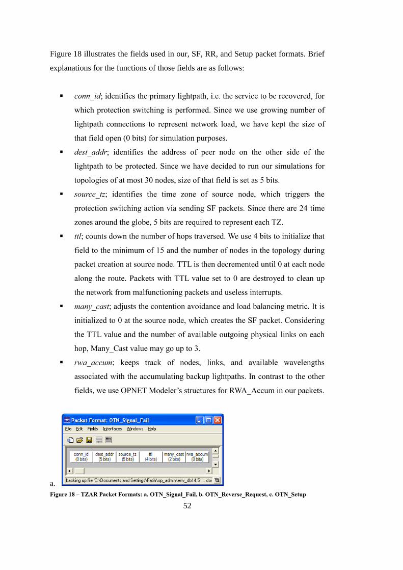
52

Figure 18 illustrates the fields used in our, SF, RR, and Setup packet formats. Brief

explanations for the functions of those fields are as follows:

conn_id; identifies the primary lightpath, i.e. the service to be recovered, for

which protection switching is performed. Since we use growing number of

lightpath connections to represent network load, we have kept the size of

that field open (0 bits) for simulation purposes.

dest_addr; identifies the address of peer node on the other side of the

lightpath to be protected. Since we have decided to run our simulations for

topologies of at most 30 nodes, size of that field is set as 5 bits.

source_tz; identifies the time zone of source node, which triggers the

protection switching action via sending SF packets. Since there are 24 time

zones around the globe, 5 bits are required to represent each TZ.

ttl; counts down the number of hops traversed. We use 4 bits to initialize that

field to the minimum of 15 and the number of nodes in the topology during

packet creation at source node. TTL is then decremented until 0 at each node

along the route. Packets with TTL value set to 0 are destroyed to clean up

the network from malfunctioning packets and useless interrupts.

many_cast; adjusts the contention avoidance and load balancing metric. It is

initialized to 0 at the source node, which creates the SF packet. Considering

the TTL value and the number of available outgoing physical links on each

hop, Many_Cast value may go up to 3.

rwa_accum; keeps track of nodes, links, and available wavelengths

associated with the accumulating backup lightpaths. In contrast to the other

fields, we use OPNET Modeler’s structures for RWA_Accum in our packets.

a.

Figure 18 – TZAR Packet Formats: a. OTN_Signal_Fail, b. OTN_Reverse_Request, c. OTN_Setup

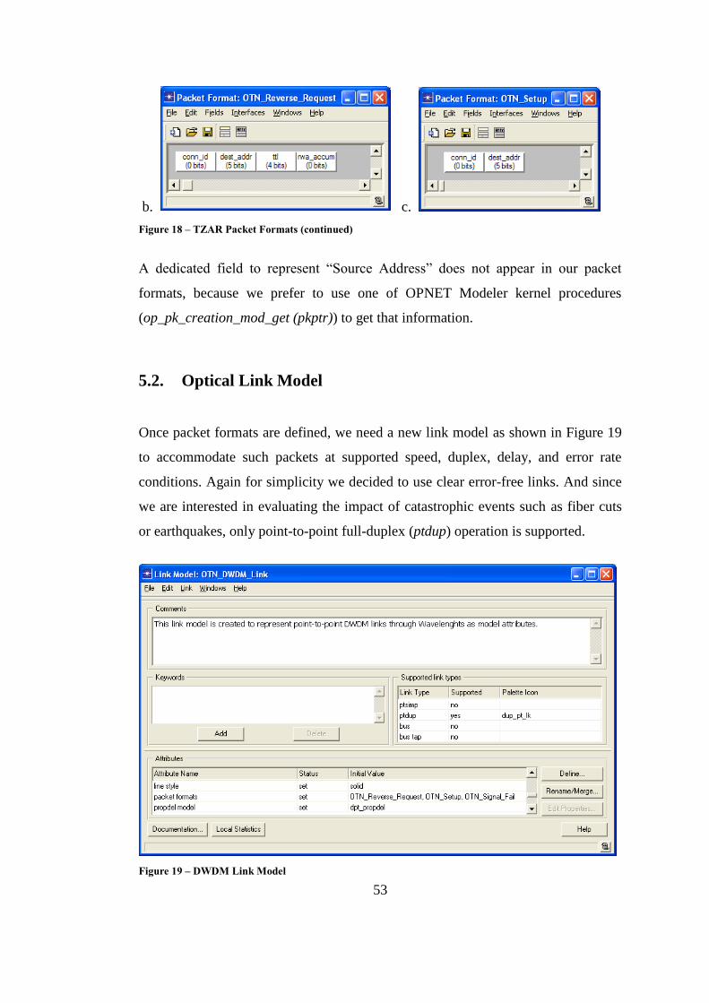
53

b. c.

Figure 18 – TZAR Packet Formats (continued)

A dedicated field to represent “Source Address” does not appear in our packet

formats, because we prefer to use one of OPNET Modeler kernel procedures

(op_pk_creation_mod_get (pkptr)) to get that information.

5.2. Optical Link Model

Once packet formats are defined, we need a new link model as shown in Figure 19

to accommodate such packets at supported speed, duplex, delay, and error rate

conditions. Again for simplicity we decided to use clear error-free links. And since

we are interested in evaluating the impact of catastrophic events such as fiber cuts

or earthquakes, only point-to-point full-duplex (ptdup) operation is supported.

Figure 19 – DWDM Link Model

54

Although we use the primary channel with an associated propagation delay model

(dpt_probdel) as a medium for OOS, we have defined a new link model attribute of

type “Compound” to assign configurable number of wavelengths for each link.

Figure 20 demonstrates that “Wavelength” attribute properties. Such a configuration

works fine for us, since we are just interested in the availability of free wavelengths

for lightpaths to be established through those links.

Figure 20 – Wavelength Attribute of DWDM Links

5.3. Processing Node Model

Geographical realities impose some restrictions on the number of conduits, in which

fiber-optic cables can be laid down. When we speak about a building as a network

center, there can be at most 4 approximations from different directions of the

building. This number may go up to 6 in case of a campus network. So, in our

simulations we have decided to model just 1 type of processing node with 6 ports.

In OPNET Modeler there are two major steps to create a new processing node. In

the first step a node model should be created using the relevant building blocks. In

the second step, process models should be created for the processor modules used in

the node model.

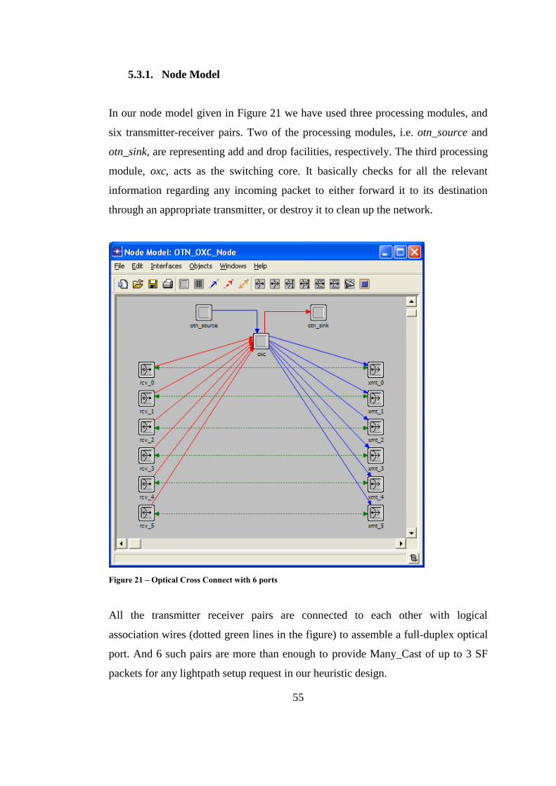
55

5.3.1. Node Model

In our node model given in Figure 21 we have used three processing modules, and

six transmitter-receiver pairs. Two of the processing modules, i.e. otn_source and

otn_sink, are representing add and drop facilities, respectively. The third processing

module, oxc, acts as the switching core. It basically checks for all the relevant

information regarding any incoming packet to either forward it to its destination

through an appropriate transmitter, or destroy it to clean up the network.

Figure 21 – Optical Cross Connect with 6 ports

All the transmitter receiver pairs are connected to each other with logical

association wires (dotted green lines in the figure) to assemble a full-duplex optical

port. And 6 such pairs are more than enough to provide Many_Cast of up to 3 SF

packets for any lightpath setup request in our heuristic design.

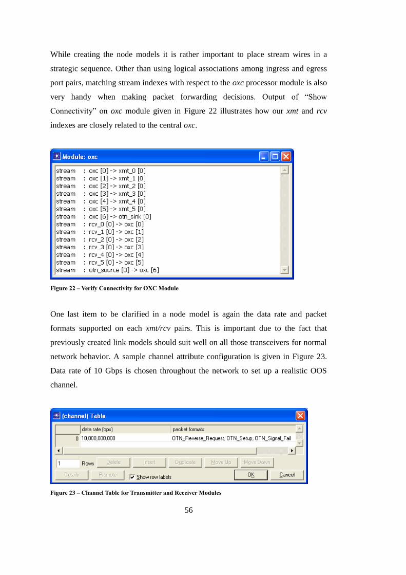
56

While creating the node models it is rather important to place stream wires in a

strategic sequence. Other than using logical associations among ingress and egress

port pairs, matching stream indexes with respect to the oxc processor module is also

very handy when making packet forwarding decisions. Output of “Show

Connectivity” on oxc module given in Figure 22 illustrates how our xmt and rcv

indexes are closely related to the central oxc.

Figure 22 – Verify Connectivity for OXC Module

One last item to be clarified in a node model is again the data rate and packet

formats supported on each xmt/rcv pairs. This is important due to the fact that

previously created link models should suit well on all those transceivers for normal

network behavior. A sample channel attribute configuration is given in Figure 23.

Data rate of 10 Gbps is chosen throughout the network to set up a realistic OOS

channel.

Figure 23 – Channel Table for Transmitter and Receiver Modules

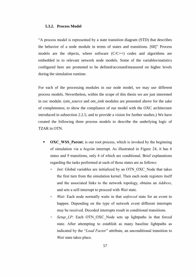
57

5.3.2. Process Model

“A process model is represented by a state transition diagram (STD) that describes

the behavior of a node module in terms of states and transitions. [68]” Process

models are the objects, where software (C/C++) codes and algorithms are

embedded in to relevant network node models. Some of the variables/statistics

configured here are promoted to be defined/accessed/measured on higher levels

during the simulation runtime.

For each of the processing modules in our node model, we may use different

process models. Nevertheless, within the scope of this thesis we are just interested

in oxc module. (otn_source and otn_sink modules are presented above for the sake

of completeness; to show the compliance of our model with the OXC architecture

introduced in subsection 2.2.5, and to provide a vision for further studies.) We have

created the following three process models to describe the underlying logic of

TZAR in OTN.

OXC_WSS_Parent; is our root process, which is invoked by the beginning

of simulation via a begsim interrupt. As illustrated in Figure 24, it has 6

states and 9 transitions, only 4 of which are conditional. Brief explanations

regarding the tasks performed at each of those states are as follows:

▫ Init: Global variables are initialized by an OTN_OXC_Node that takes

the first turn from the simulation kernel. Then each node registers itself

and the associated links to the network topology, obtains an Address,

and sets a self-interrupt to proceed with Wait state.

▫ Wait: Each node normally waits in that unforced state for an event to

happen. Depending on the type of network event different interrupts

may be received. Decoded interrupts result in conditional transitions.

▫ Setup_LP: Each OTN_OXC_Node sets up lightpaths in that forced

state. After attempting to establish as many baseline lightpaths as

indicated by the “Load Factor” attribute, an unconditional transition to

Wait state takes place.

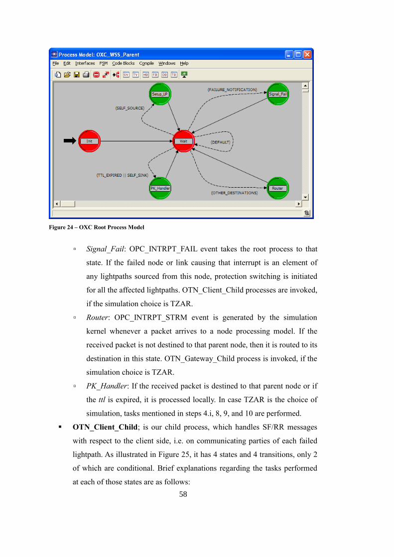
58

Figure 24 – OXC Root Process Model

▫ Signal_Fail: OPC_INTRPT_FAIL event takes the root process to that

state. If the failed node or link causing that interrupt is an element of

any lightpaths sourced from this node, protection switching is initiated

for all the affected lightpaths. OTN_Client_Child processes are invoked,

if the simulation choice is TZAR.

▫ Router: OPC_INTRPT_STRM event is generated by the simulation

kernel whenever a packet arrives to a node processing model. If the

received packet is not destined to that parent node, then it is routed to its

destination in this state. OTN_Gateway_Child process is invoked, if the

simulation choice is TZAR.

▫ PK_Handler: If the received packet is destined to that parent node or if

the ttl is expired, it is processed locally. In case TZAR is the choice of

simulation, tasks mentioned in steps 4.i, 8, 9, and 10 are performed.

OTN_Client_Child; is our child process, which handles SF/RR messages

with respect to the client side, i.e. on communicating parties of each failed

lightpath. As illustrated in Figure 25, it has 4 states and 4 transitions, only 2

of which are conditional. Brief explanations regarding the tasks performed

at each of those states are as follows:

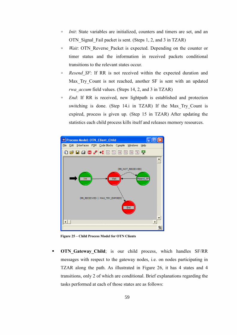
59

▫ Init: State variables are initialized, counters and timers are set, and an

OTN_Signal_Fail packet is sent. (Steps 1, 2, and 3 in TZAR)

▫ Wait: OTN_Reverse_Packet is expected. Depending on the counter or

timer status and the information in received packets conditional

transitions to the relevant states occur.

▫ Resend_SF: If RR is not received within the expected duration and

Max_Try_Count is not reached, another SF is sent with an updated

rwa_accum field values. (Steps 14, 2, and 3 in TZAR)

▫ End: If RR is received, new lightpath is established and protection

switching is done. (Step 14.i in TZAR) If the Max_Try_Count is

expired, process is given up. (Step 15 in TZAR) After updating the

statistics each child process kills itself and releases memory resources.

Figure 25 – Child Process Model for OTN Clients

OTN_Gateway_Child; is our child process, which handles SF/RR

messages with respect to the gateway nodes, i.e. on nodes participating in

TZAR along the path. As illustrated in Figure 26, it has 4 states and 4

transitions, only 2 of which are conditional. Brief explanations regarding the

tasks performed at each of those states are as follows:

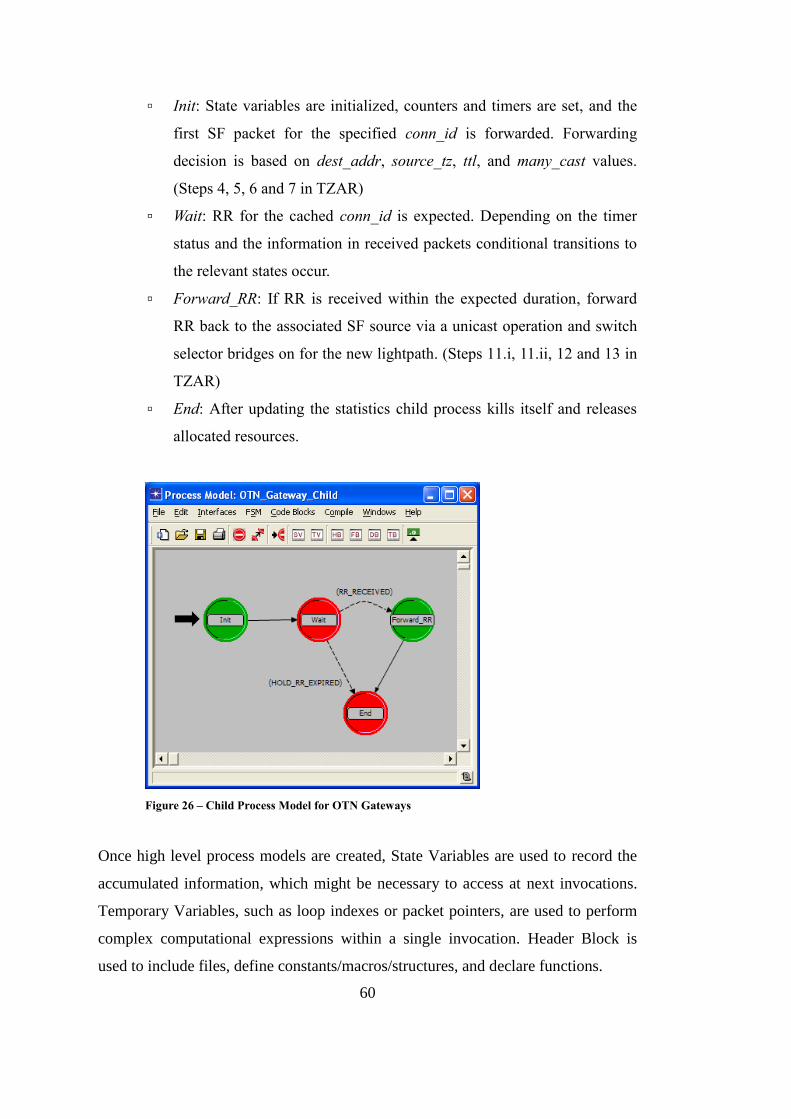
60

▫ Init: State variables are initialized, counters and timers are set, and the

first SF packet for the specified conn_id is forwarded. Forwarding

decision is based on dest_addr, source_tz, ttl, and many_cast values.

(Steps 4, 5, 6 and 7 in TZAR)

▫ Wait: RR for the cached conn_id is expected. Depending on the timer

status and the information in received packets conditional transitions to

the relevant states occur.

▫ Forward_RR: If RR is received within the expected duration, forward

RR back to the associated SF source via a unicast operation and switch

selector bridges on for the new lightpath. (Steps 11.i, 11.ii, 12 and 13 in

TZAR)

▫ End: After updating the statistics child process kills itself and releases

allocated resources.

Figure 26 – Child Process Model for OTN Gateways

Once high level process models are created, State Variables are used to record the

accumulated information, which might be necessary to access at next invocations.

Temporary Variables, such as loop indexes or packet pointers, are used to perform

complex computational expressions within a single invocation. Header Block is

used to include files, define constants/macros/structures, and declare functions.

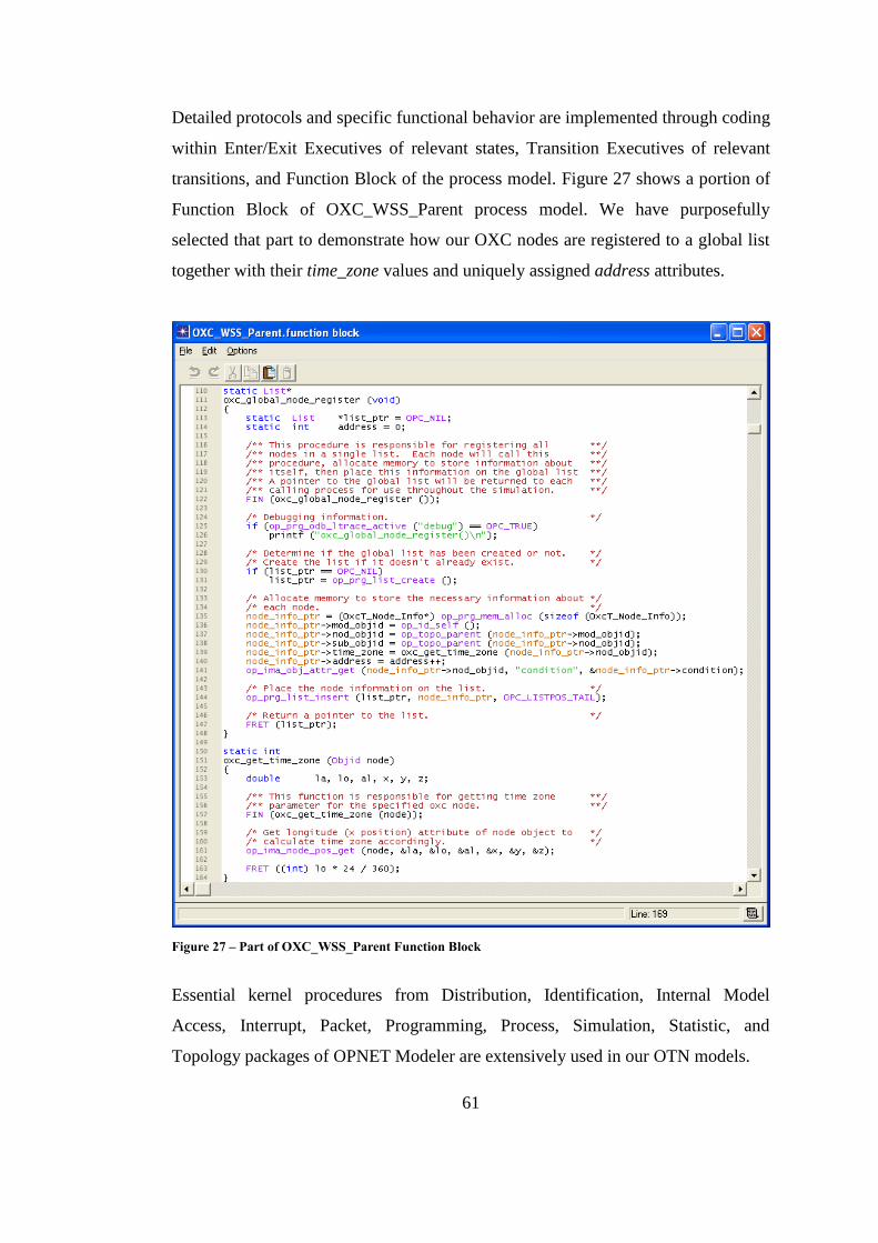
61

Detailed protocols and specific functional behavior are implemented through coding

within Enter/Exit Executives of relevant states, Transition Executives of relevant

transitions, and Function Block of the process model. Figure 27 shows a portion of

Function Block of OXC_WSS_Parent process model. We have purposefully

selected that part to demonstrate how our OXC nodes are registered to a global list

together with their time_zone values and uniquely assigned address attributes.

Figure 27 – Part of OXC_WSS_Parent Function Block

Essential kernel procedures from Distribution, Identification, Internal Model

Access, Interrupt, Packet, Programming, Process, Simulation, Statistic, and

Topology packages of OPNET Modeler are extensively used in our OTN models.

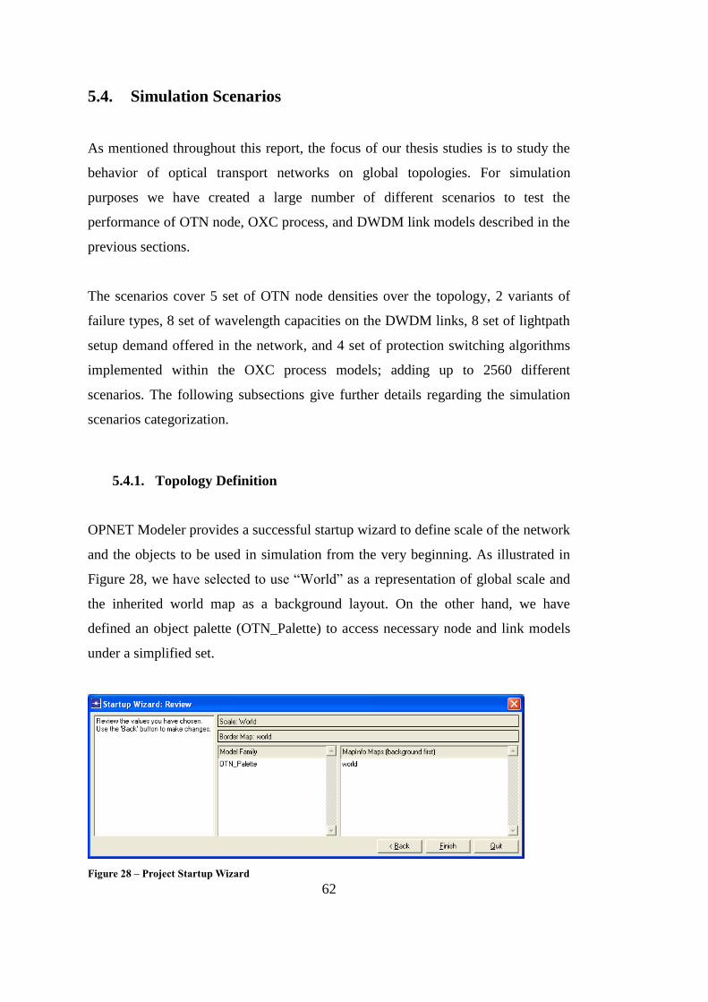
62

5.4. Simulation Scenarios

As mentioned throughout this report, the focus of our thesis studies is to study the

behavior of optical transport networks on global topologies. For simulation

purposes we have created a large number of different scenarios to test the

performance of OTN node, OXC process, and DWDM link models described in the

previous sections.

The scenarios cover 5 set of OTN node densities over the topology, 2 variants of

failure types, 8 set of wavelength capacities on the DWDM links, 8 set of lightpath

setup demand offered in the network, and 4 set of protection switching algorithms

implemented within the OXC process models; adding up to 2560 different

scenarios. The following subsections give further details regarding the simulation

scenarios categorization.

5.4.1. Topology Definition

OPNET Modeler provides a successful startup wizard to define scale of the network

and the objects to be used in simulation from the very beginning. As illustrated in

Figure 28, we have selected to use “World” as a representation of global scale and

the inherited world map as a background layout. On the other hand, we have

defined an object palette (OTN_Palette) to access necessary node and link models

under a simplified set.

Figure 28 – Project Startup Wizard

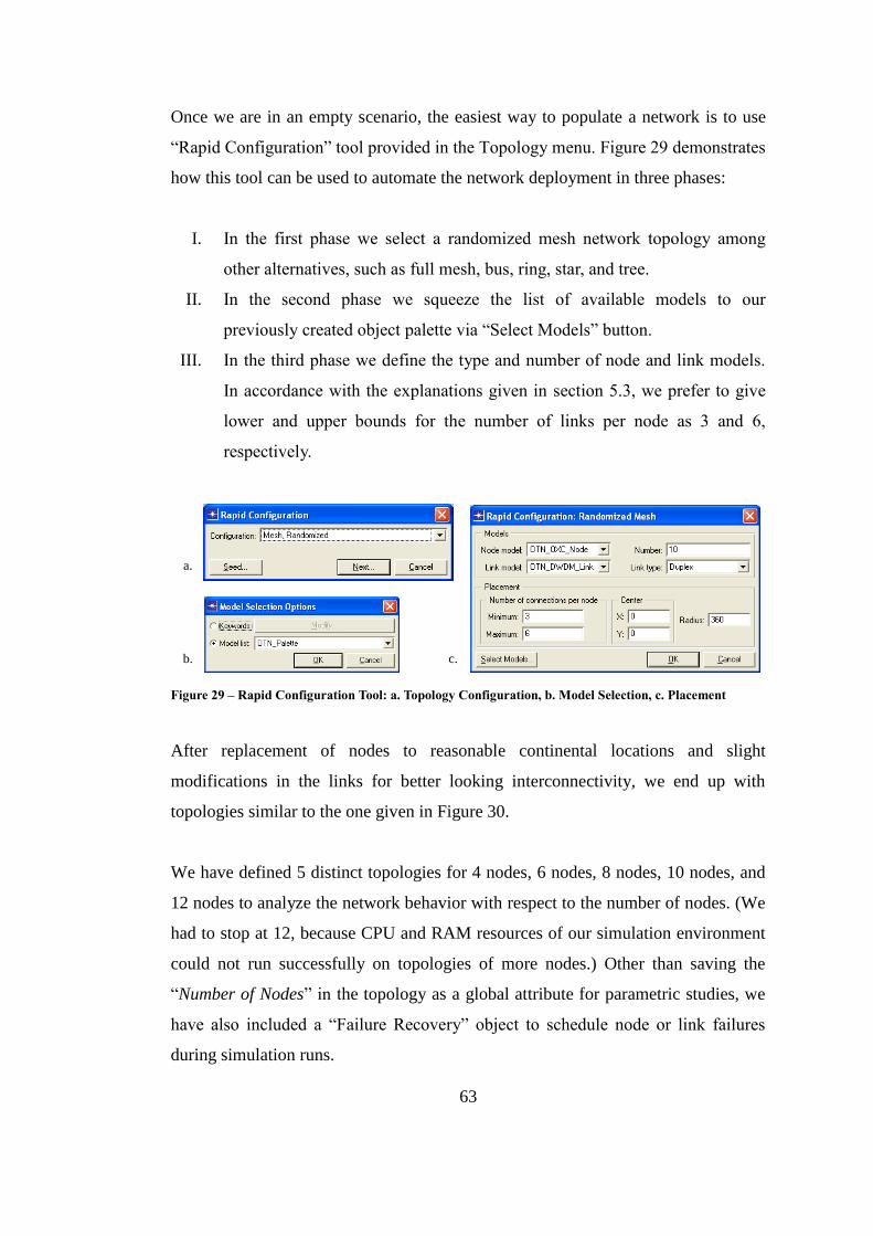
63

Once we are in an empty scenario, the easiest way to populate a network is to use

“Rapid Configuration” tool provided in the Topology menu. Figure 29 demonstrates

how this tool can be used to automate the network deployment in three phases:

I. In the first phase we select a randomized mesh network topology among

other alternatives, such as full mesh, bus, ring, star, and tree.

II. In the second phase we squeeze the list of available models to our

previously created object palette via “Select Models” button.

III. In the third phase we define the type and number of node and link models.

In accordance with the explanations given in section 5.3, we prefer to give

lower and upper bounds for the number of links per node as 3 and 6,

respectively.

a.

b. c.

Figure 29 – Rapid Configuration Tool: a. Topology Configuration, b. Model Selection, c. Placement

After replacement of nodes to reasonable continental locations and slight

modifications in the links for better looking interconnectivity, we end up with

topologies similar to the one given in Figure 30.

We have defined 5 distinct topologies for 4 nodes, 6 nodes, 8 nodes, 10 nodes, and

12 nodes to analyze the network behavior with respect to the number of nodes. (We

had to stop at 12, because CPU and RAM resources of our simulation environment

could not run successfully on topologies of more nodes.) Other than saving the

“Number of Nodes” in the topology as a global attribute for parametric studies, we

have also included a “Failure Recovery” object to schedule node or link failures

during simulation runs.

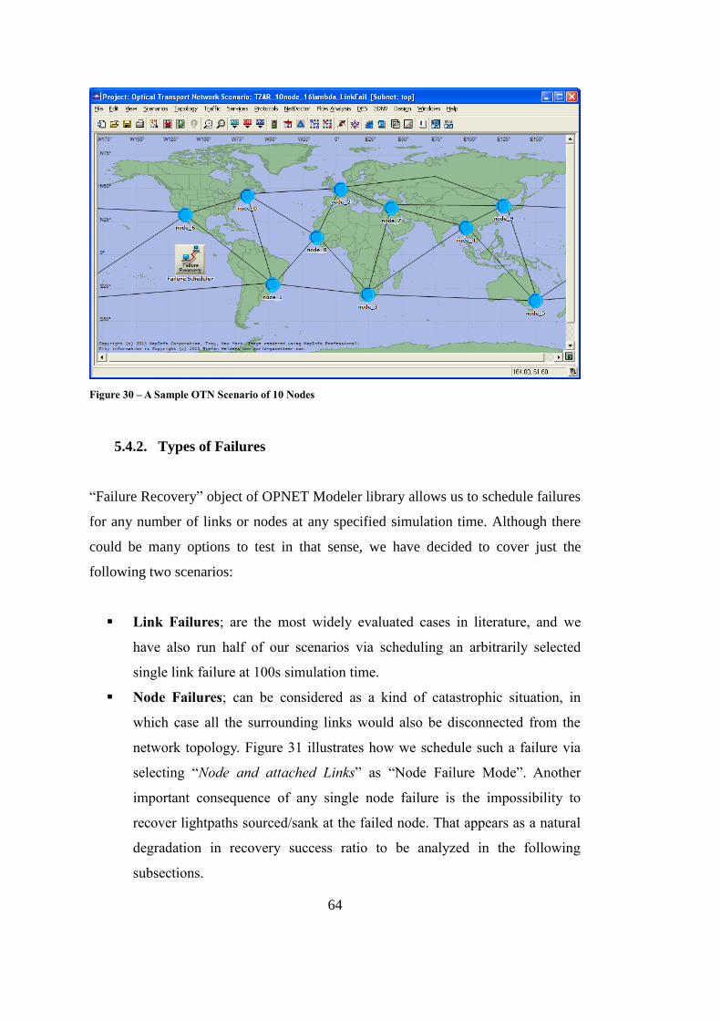
64

Figure 30 – A Sample OTN Scenario of 10 Nodes

5.4.2. Types of Failures

“Failure Recovery” object of OPNET Modeler library allows us to schedule failures

for any number of links or nodes at any specified simulation time. Although there

could be many options to test in that sense, we have decided to cover just the

following two scenarios:

Link Failures; are the most widely evaluated cases in literature, and we

have also run half of our scenarios via scheduling an arbitrarily selected

single link failure at 100s simulation time.

Node Failures; can be considered as a kind of catastrophic situation, in

which case all the surrounding links would also be disconnected from the

network topology. Figure 31 illustrates how we schedule such a failure via

selecting “Node and attached Links” as “Node Failure Mode”. Another

important consequence of any single node failure is the impossibility to

recover lightpaths sourced/sank at the failed node. That appears as a natural

degradation in recovery success ratio to be analyzed in the following

subsections.

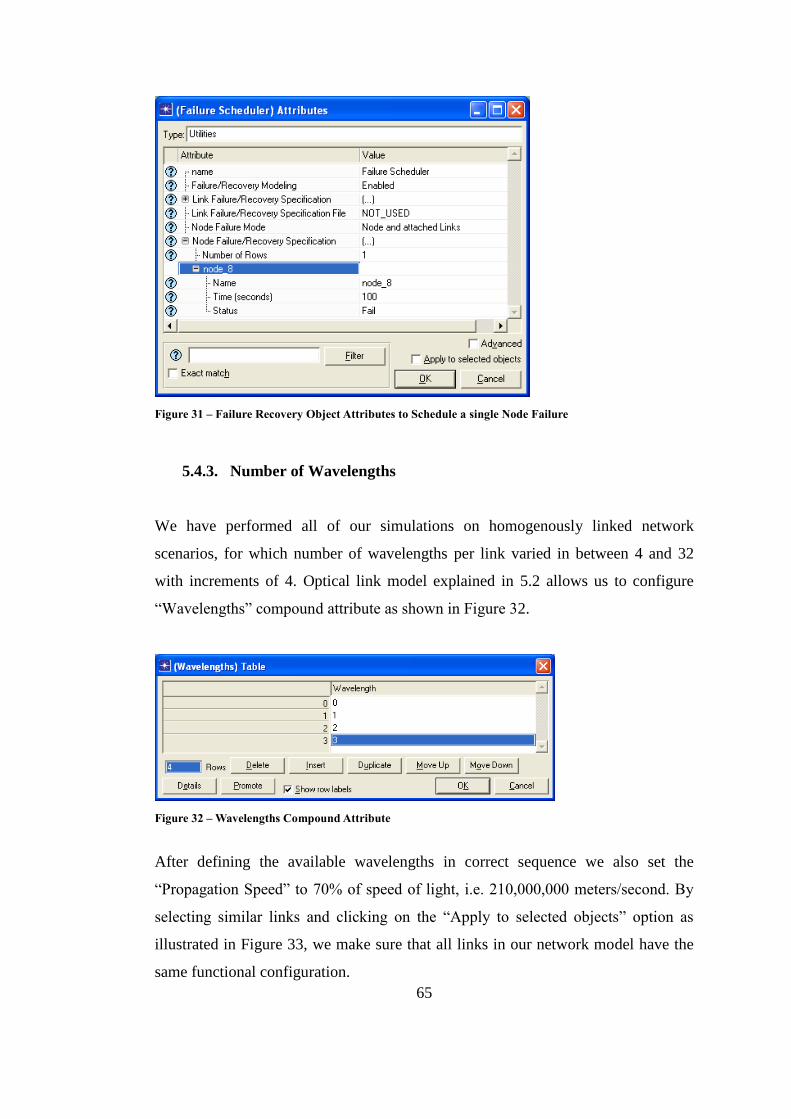
65

Figure 31 – Failure Recovery Object Attributes to Schedule a single Node Failure

5.4.3. Number of Wavelengths

We have performed all of our simulations on homogenously linked network

scenarios, for which number of wavelengths per link varied in between 4 and 32

with increments of 4. Optical link model explained in 5.2 allows us to configure

“Wavelengths” compound attribute as shown in Figure 32.

Figure 32 – Wavelengths Compound Attribute

After defining the available wavelengths in correct sequence we also set the

“Propagation Speed” to 70% of speed of light, i.e. 210,000,000 meters/second. By

selecting similar links and clicking on the “Apply to selected objects” option as

illustrated in Figure 33, we make sure that all links in our network model have the

same functional configuration.

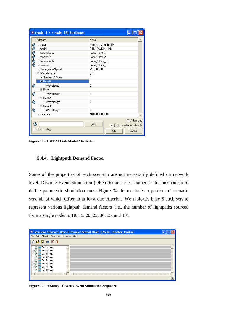
66

Figure 33 – DWDM Link Model Attributes

5.4.4. Lightpath Demand Factor

Some of the properties of each scenario are not necessarily defined on network

level. Discrete Event Simulation (DES) Sequence is another useful mechanism to

define parametric simulation runs. Figure 34 demonstrates a portion of scenario

sets, all of which differ in at least one criterion. We typically have 8 such sets to

represent various lightpath demand factors (i.e., the number of lightpaths sourced

from a single node: 5, 10, 15, 20, 25, 30, 35, and 40).

Figure 34 – A Sample Discrete Event Simulation Sequence

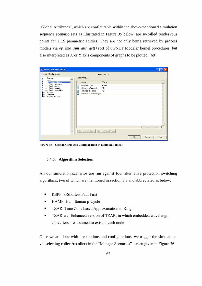
67

“Global Attributes”, which are configurable within the above-mentioned simulation

sequence scenario sets as illustrated in Figure 35 below, are so-called rendezvous

points for DES parametric studies. They are not only being retrieved by process

models via op_ima_sim_attr_get() sort of OPNET Modeler kernel procedures, but

also interpreted as X or Y axis components of graphs to be plotted. [69]

Figure 35 – Global Attributes Configuration in a Simulation Set

5.4.5. Algorithm Selection

All our simulation scenarios are run against four alternative protection switching

algorithms, two of which are mentioned in section 3.3 and abbreviated as below.

KSPF: k-Shortest Path First

HAMP: Hamiltonian p-Cycle

TZAR: Time Zone based Approximation to Ring

TZAR-wc: Enhanced version of TZAR, in which embedded wavelength

converters are assumed to exist at each node

Once we are done with preparations and configurations, we trigger the simulations

via selecting collect/recollect in the “Manage Scenarios” screen given in Figure 36.

68

Figure 36 – Manage Scenarios Screen

5.5. Results Collected

During the simulation runs we can follow the summary of happenings, such as

status and duration of the runs as well as the number of events and consumed

memory for each run, through a popped-up screen as given in Figure 37. We

recognize that the simulation runs of 4 node topologies with 4 supported

wavelengths and 5 lightpath setup demands complete within sub-second durations

for approximately 150 events. On the other extreme, simulation runs of 12 node

topologies with 32 supported wavelengths and 40 lightpath setup demands complete

in more than a minute period for approximately 4250 events. These numbers give us

rough estimations regarding the proper run of the simulations. For detailed analyses

of the results collected we have to switch to the “Results Browser”, which will be

covered in the following subsections.

Figure 37 – DES Execution Manager Window

69

5.5.1. Confidence Interval

Although common sense and a little bit intuition would agree, that for instance

blocking probably should decrease with increasing number of wavelengths, we have

to validate any behavior of our process models’ equivalence to real systems. Our

measurements based on incremental analyses for alternative algorithms aim to

achieve a plausible degree of confidence.

To ensure a sufficiently large number of independent experiments we have used

altering random number generator seeds for different sets of simulation scenarios. 3

stochastic functions that we have used are dependent on those selected seeds:

i. Order of primary lightpaths’ setup depends on a self-triggered interrupt

randomly distributed over 5-15 seconds as illustrated in Figure 38.a.

ii. Destination address of any lightpath to be established is set to be randomly

generated among available destination nodes in the topology as illustrated in

Figure 38.b.

iii. Signal_Fail many_casting operation in TZAR proceeds with a random

selection among candidate neighbors as illustrated in Figure 38.c.

Since it is not possible to run infinite number of simulations to get the true mean μ

for any scalar statistic, we are interested in the degree of precision that can be

approximated via collected samples through N simulations. How good such

approximations are done determines the confidence level of the results collected.

For large enough N (typically more than 30), our randomized statistic is assumed

to have a normal distribution with a mean approaching to true mean μ. And

according to central limit theorem, variance of is 2 ⁄ , where 2 is the true

variance. Standardized normal variable Z is then defined as ⁄ , where the

distance of a particular sample from μ in terms of the number of standard

deviations has a zero mean and a unity standard deviation. By the way, we can

speak about a probability that a sample result is within a bounded distance of μ as

formulated in 5.1 below.

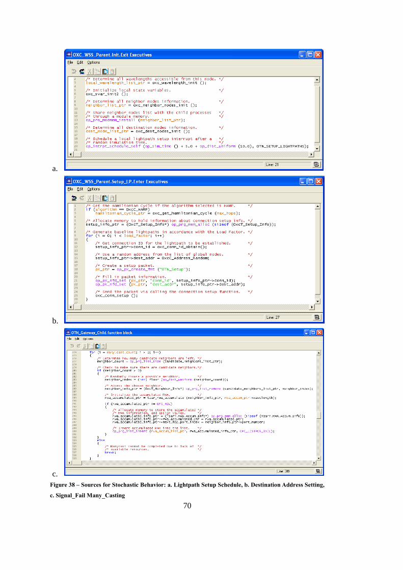
70

a.

b.

c.

Figure 38 – Sources for Stochastic Behavior: a. Lightpath Setup Schedule, b. Destination Address Setting,

c. Signal_Fail Many_Casting

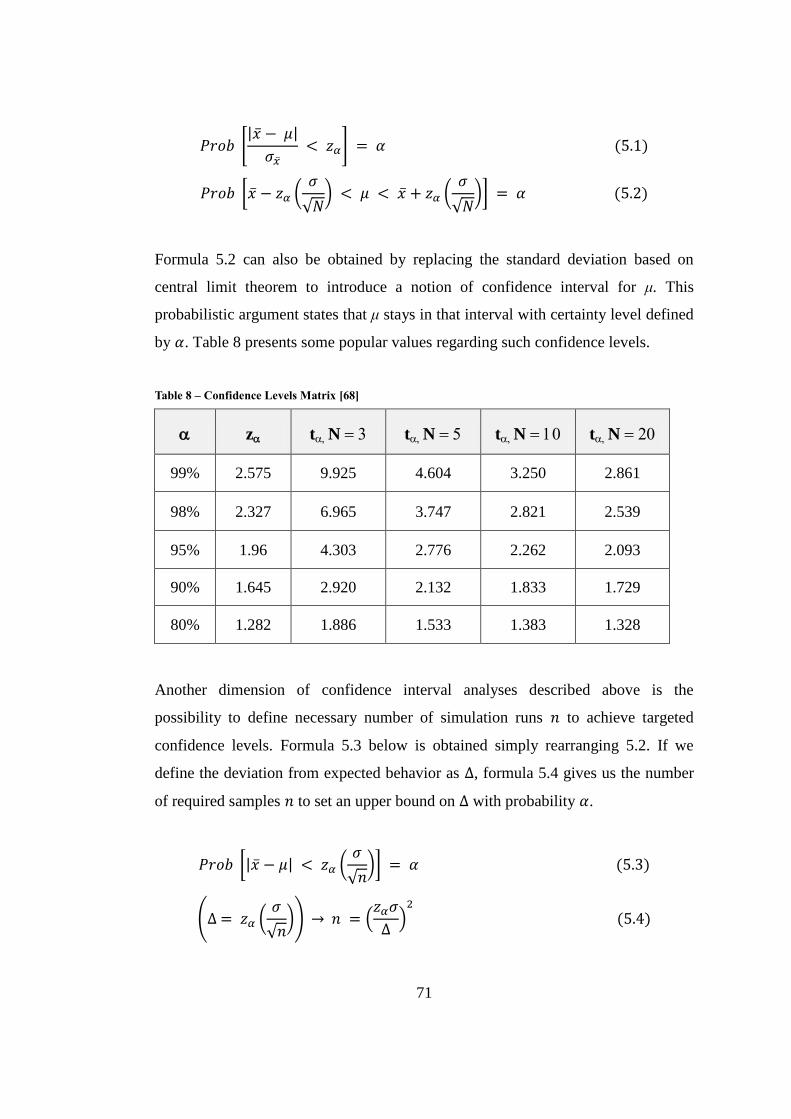
71

[| |

] =

[ (

√ ) + (

√ )] =

Formula 5.2 can also be obtained by replacing the standard deviation based on

central limit theorem to introduce a notion of confidence interval for μ. This

probabilistic argument states that μ stays in that interval with certainty level defined

by . Table 8 presents some popular values regarding such confidence levels.

Table 8 – Confidence Levels Matrix [68]

z tN tN tN tN

99% 2.575 9.925 4.604 3.250 2.861

98% 2.327 6.965 3.747 2.821 2.539

95% 1.96 4.303 2.776 2.262 2.093

90% 1.645 2.920 2.132 1.833 1.729

80% 1.282 1.886 1.533 1.383 1.328

Another dimension of confidence interval analyses described above is the

possibility to define necessary number of simulation runs to achieve targeted

confidence levels. Formula 5.3 below is obtained simply rearranging 5.2. If we

define the deviation from expected behavior as , formula 5.4 gives us the number

of required samples to set an upper bound on with probability .

[| | (

√ )] =

( = (

√ )) = (

)2

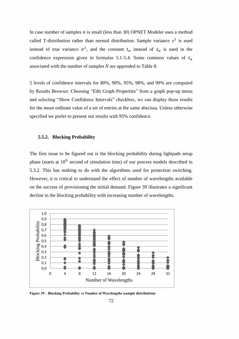
72

In case number of samples is small (less than 30) OPNET Modeler uses a method

called T-distribution rather than normal distribution. Sample variance 2 is used

instead of true variance 2, and the constant instead of is used in the

confidence expression given in formulas 5.1-5.4. Some common values of

associated with the number of samples N are appended to Table 8.

5 levels of confidence intervals for 80%, 90%, 95%, 98%, and 99% are computed

by Results Browser. Choosing “Edit Graph Properties” from a graph pop-up menu

and selecting “Show Confidence Intervals” checkbox, we can display these results

for the mean ordinate value of a set of entries at the same abscissa. Unless otherwise

specified we prefer to present our results with 95% confidence.

5.5.2. Blocking Probability

The first issue to be figured out is the blocking probability during lightpath setup

phase (starts at 10th

second of simulation time) of our process models described in

5.3.2. This has nothing to do with the algorithms used for protection switching.

However, it is critical to understand the effect of number of wavelengths available

on the success of provisioning the initial demand. Figure 39 illustrates a significant

decline in the blocking probability with increasing number of wavelengths.

Figure 39 – Blocking Probability vs Number of Wavelengths (sample distribution)

0,0

0,1

0,2

0,3

0,4

0,5

0,6

0,7

0,8

0,9

1,0

0 4 8 12 16 20 24 28 32

Blo

ckin

g P

robab

ilit

y

Number of Wavelengths

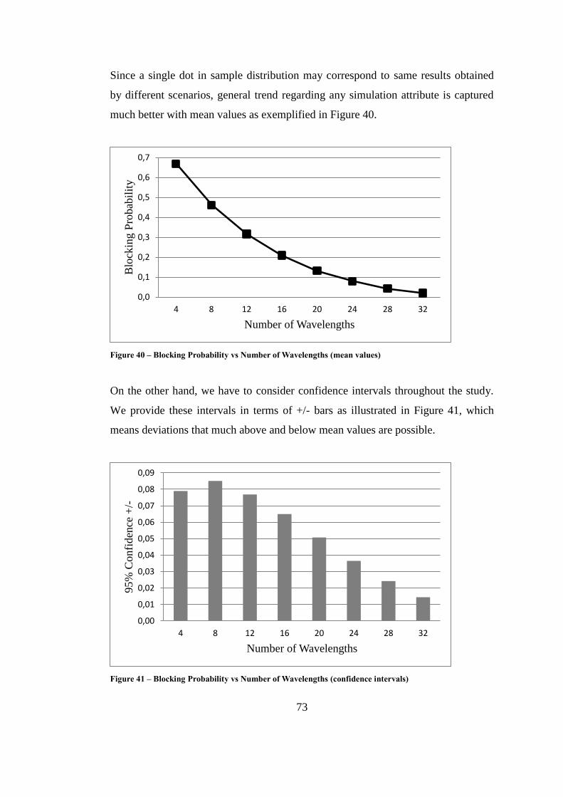
73

Since a single dot in sample distribution may correspond to same results obtained

by different scenarios, general trend regarding any simulation attribute is captured

much better with mean values as exemplified in Figure 40.

Figure 40 – Blocking Probability vs Number of Wavelengths (mean values)

On the other hand, we have to consider confidence intervals throughout the study.

We provide these intervals in terms of +/- bars as illustrated in Figure 41, which

means deviations that much above and below mean values are possible.

Figure 41 – Blocking Probability vs Number of Wavelengths (confidence intervals)

0,0

0,1

0,2

0,3

0,4

0,5

0,6

0,7

4 8 12 16 20 24 28 32

Blo

ckin

g P

robab

ilit

y


0,00

0,01

0,02

0,03

0,04

0,05

0,06

0,07

0,08

0,09

4 8 12 16 20 24 28 32

95%

Con

fiden

ce +

/-


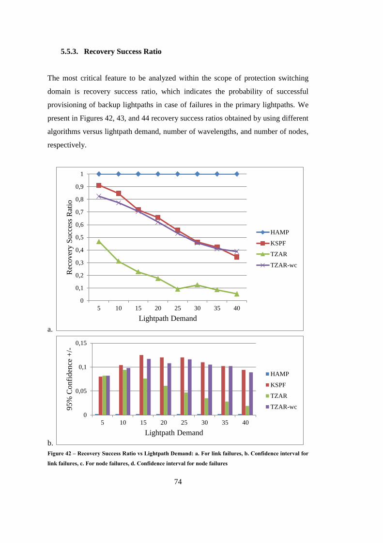
74

5.5.3. Recovery Success Ratio

The most critical feature to be analyzed within the scope of protection switching

domain is recovery success ratio, which indicates the probability of successful

provisioning of backup lightpaths in case of failures in the primary lightpaths. We

present in Figures 42, 43, and 44 recovery success ratios obtained by using different

algorithms versus lightpath demand, number of wavelengths, and number of nodes,

respectively.

a.

b.

Figure 42 – Recovery Success Ratio vs Lightpath Demand: a. For link failures, b. Confidence interval for

link failures, c. For node failures, d. Confidence interval for node failures

0

0,1

0,2

0,3

0,4

0,5

0,6

0,7

0,8

0,9

1

5 10 15 20 25 30 35 40

Rec

over

y S

ucc

ess

Rat

io

Lightpath Demand

HAMP

KSPF

TZAR

TZAR-wc

0

0,05

0,1

0,15

5 10 15 20 25 30 35 40

95%

Confi

den

ce +

/-

Lightpath Demand

HAMP

KSPF

TZAR

TZAR-wc

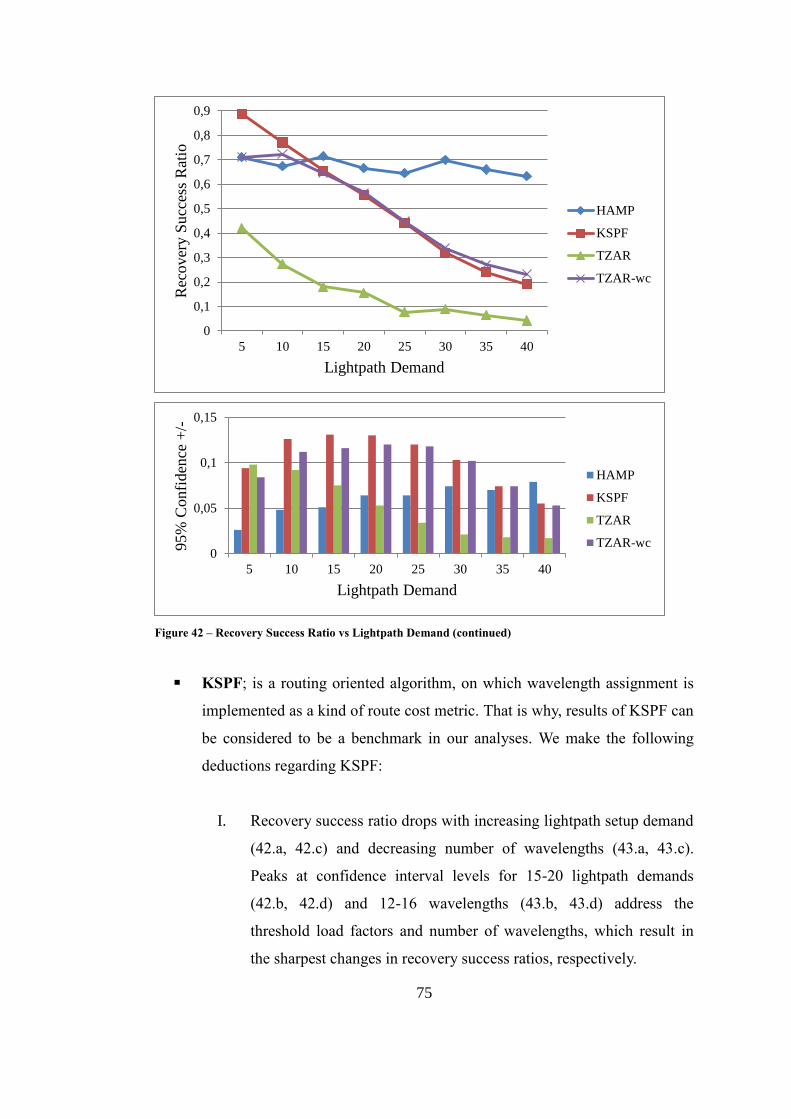
75

Figure 42 – Recovery Success Ratio vs Lightpath Demand (continued)

KSPF; is a routing oriented algorithm, on which wavelength assignment is

implemented as a kind of route cost metric. That is why, results of KSPF can

be considered to be a benchmark in our analyses. We make the following

deductions regarding KSPF:

I. Recovery success ratio drops with increasing lightpath setup demand

(42.a, 42.c) and decreasing number of wavelengths (43.a, 43.c).

Peaks at confidence interval levels for 15-20 lightpath demands

(42.b, 42.d) and 12-16 wavelengths (43.b, 43.d) address the

threshold load factors and number of wavelengths, which result in

the sharpest changes in recovery success ratios, respectively.

0

0,1

0,2

0,3

0,4

0,5

0,6

0,7

0,8

0,9

5 10 15 20 25 30 35 40

Rec

over

y S

ucc

ess

Rat

io

Lightpath Demand

HAMP

KSPF

TZAR

TZAR-wc

0

0,05

0,1

0,15

5 10 15 20 25 30 35 40

95%

Confi

den

ce +

/-

Lightpath Demand

HAMP

KSPF

TZAR

TZAR-wc

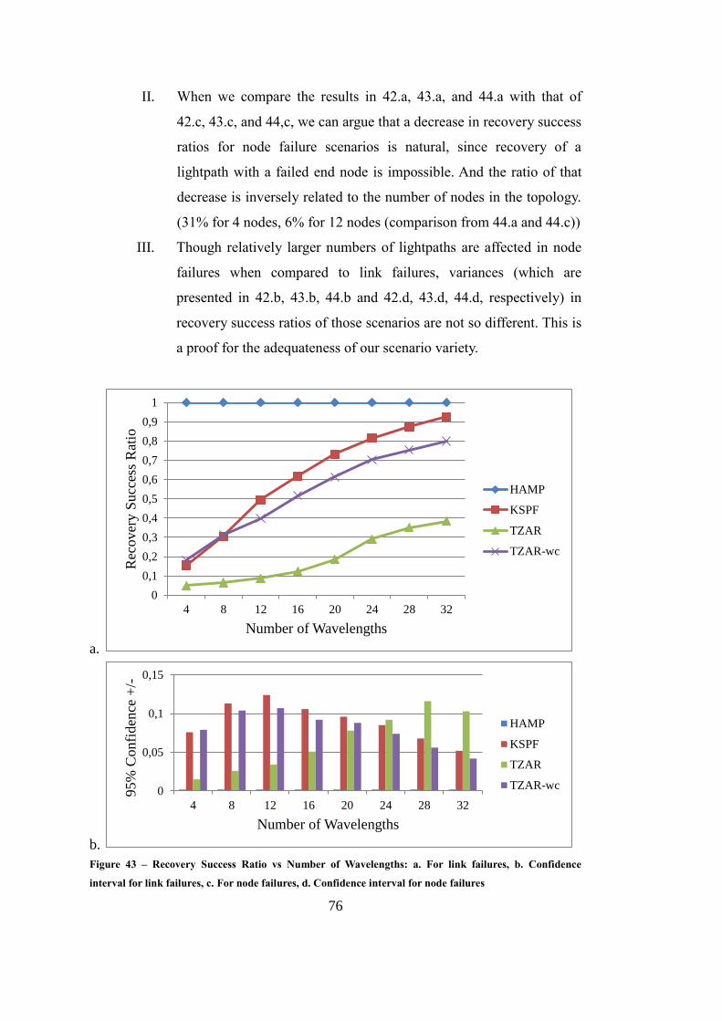
76

II. When we compare the results in 42.a, 43.a, and 44.a with that of

42.c, 43.c, and 44,c, we can argue that a decrease in recovery success

ratios for node failure scenarios is natural, since recovery of a

lightpath with a failed end node is impossible. And the ratio of that

decrease is inversely related to the number of nodes in the topology.

(31% for 4 nodes, 6% for 12 nodes (comparison from 44.a and 44.c))

III. Though relatively larger numbers of lightpaths are affected in node

failures when compared to link failures, variances (which are

presented in 42.b, 43.b, 44.b and 42.d, 43.d, 44.d, respectively) in

recovery success ratios of those scenarios are not so different. This is

a proof for the adequateness of our scenario variety.

a.

b.

Figure 43 – Recovery Success Ratio vs Number of Wavelengths: a. For link failures, b. Confidence

interval for link failures, c. For node failures, d. Confidence interval for node failures

0

0,1

0,2

0,3

0,4

0,5

0,6

0,7

0,8

0,9

1

4 8 12 16 20 24 28 32

Rec

over

y S

ucc

ess

Rat

io


HAMP

KSPF

TZAR

TZAR-wc

0

0,05

0,1

0,15

4 8 12 16 20 24 28 32

95%

Confi

den

ce +

/-


HAMP

KSPF

TZAR

TZAR-wc

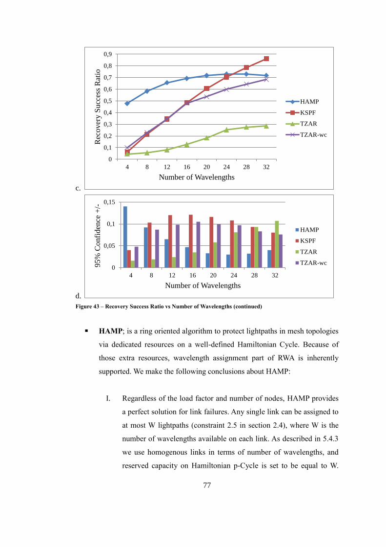
77

c.

d.

Figure 43 – Recovery Success Ratio vs Number of Wavelengths (continued)

HAMP; is a ring oriented algorithm to protect lightpaths in mesh topologies

via dedicated resources on a well-defined Hamiltonian Cycle. Because of

those extra resources, wavelength assignment part of RWA is inherently

supported. We make the following conclusions about HAMP:

I. Regardless of the load factor and number of nodes, HAMP provides

a perfect solution for link failures. Any single link can be assigned to

at most W lightpaths (constraint 2.5 in section 2.4), where W is the

number of wavelengths available on each link. As described in 5.4.3

we use homogenous links in terms of number of wavelengths, and

reserved capacity on Hamiltonian p-Cycle is set to be equal to W.

0

0,1

0,2

0,3

0,4

0,5

0,6

0,7

0,8

0,9

4 8 12 16 20 24 28 32

Rec

over

y S

ucc

ess

Rat

io


HAMP

KSPF

TZAR

TZAR-wc

0

0,05

0,1

0,15

4 8 12 16 20 24 28 32

95%

Confi

den

ce +

/-


HAMP

KSPF

TZAR

TZAR-wc

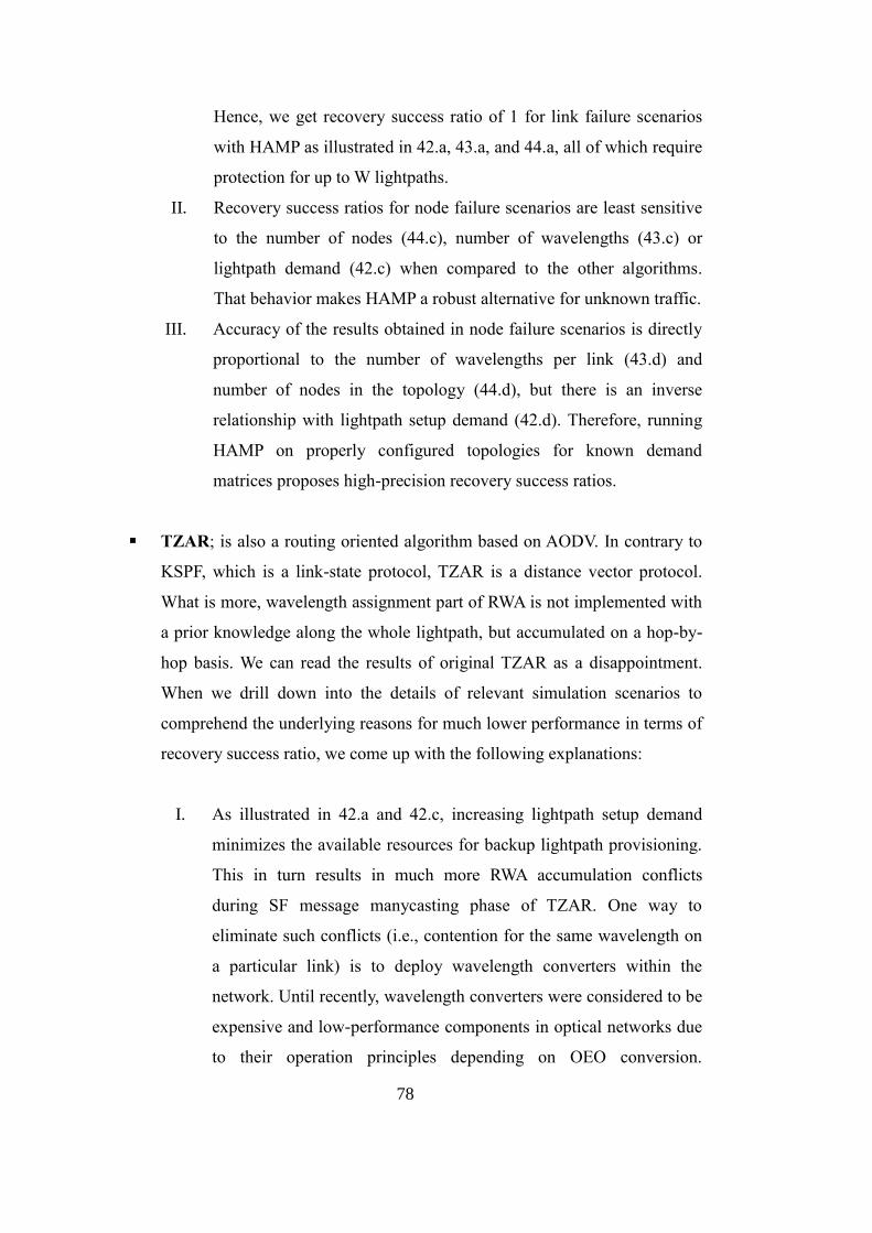
78

Hence, we get recovery success ratio of 1 for link failure scenarios

with HAMP as illustrated in 42.a, 43.a, and 44.a, all of which require

protection for up to W lightpaths.

II. Recovery success ratios for node failure scenarios are least sensitive

to the number of nodes (44.c), number of wavelengths (43.c) or

lightpath demand (42.c) when compared to the other algorithms.

That behavior makes HAMP a robust alternative for unknown traffic.

III. Accuracy of the results obtained in node failure scenarios is directly

proportional to the number of wavelengths per link (43.d) and

number of nodes in the topology (44.d), but there is an inverse

relationship with lightpath setup demand (42.d). Therefore, running

HAMP on properly configured topologies for known demand

matrices proposes high-precision recovery success ratios.

TZAR; is also a routing oriented algorithm based on AODV. In contrary to

KSPF, which is a link-state protocol, TZAR is a distance vector protocol.

What is more, wavelength assignment part of RWA is not implemented with

a prior knowledge along the whole lightpath, but accumulated on a hop-by-

hop basis. We can read the results of original TZAR as a disappointment.

When we drill down into the details of relevant simulation scenarios to

comprehend the underlying reasons for much lower performance in terms of

recovery success ratio, we come up with the following explanations:

I. As illustrated in 42.a and 42.c, increasing lightpath setup demand

minimizes the available resources for backup lightpath provisioning.

This in turn results in much more RWA accumulation conflicts

during SF message manycasting phase of TZAR. One way to

eliminate such conflicts (i.e., contention for the same wavelength on

a particular link) is to deploy wavelength converters within the

network. Until recently, wavelength converters were considered to be

expensive and low-performance components in optical networks due

to their operation principles depending on OEO conversion.

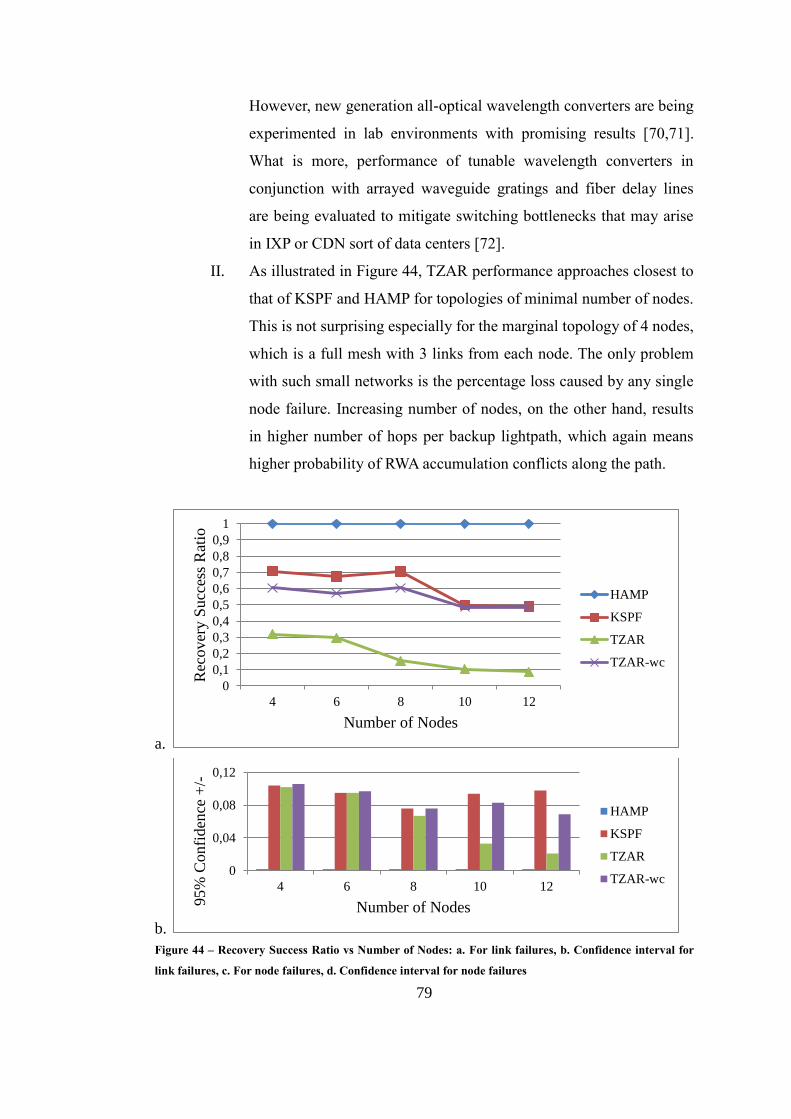
79

However, new generation all-optical wavelength converters are being

experimented in lab environments with promising results [70,71].

What is more, performance of tunable wavelength converters in

conjunction with arrayed waveguide gratings and fiber delay lines

are being evaluated to mitigate switching bottlenecks that may arise

in IXP or CDN sort of data centers [72].

II. As illustrated in Figure 44, TZAR performance approaches closest to

that of KSPF and HAMP for topologies of minimal number of nodes.

This is not surprising especially for the marginal topology of 4 nodes,

which is a full mesh with 3 links from each node. The only problem

with such small networks is the percentage loss caused by any single

node failure. Increasing number of nodes, on the other hand, results

in higher number of hops per backup lightpath, which again means

higher probability of RWA accumulation conflicts along the path.

a.

b.

Figure 44 – Recovery Success Ratio vs Number of Nodes: a. For link failures, b. Confidence interval for


0

0,1

0,2

0,3

0,4

0,5

0,6

0,7

0,8

0,9

1

4 6 8 10 12

Rec

over

y S

ucc

ess

Rat

io

Number of Nodes

HAMP

KSPF

TZAR

TZAR-wc

0

0,04

0,08

0,12

4 6 8 10 12

95%

Confi

den

ce +

/-

Number of Nodes

HAMP

KSPF

TZAR

TZAR-wc

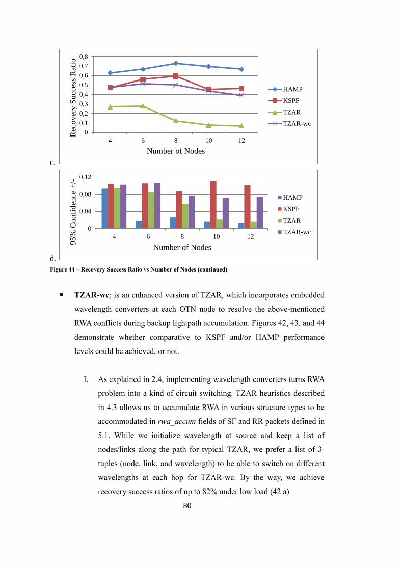
80

c.

d.

Figure 44 – Recovery Success Ratio vs Number of Nodes (continued)

TZAR-wc; is an enhanced version of TZAR, which incorporates embedded

wavelength converters at each OTN node to resolve the above-mentioned

RWA conflicts during backup lightpath accumulation. Figures 42, 43, and 44

demonstrate whether comparative to KSPF and/or HAMP performance

levels could be achieved, or not.

I. As explained in 2.4, implementing wavelength converters turns RWA

problem into a kind of circuit switching. TZAR heuristics described

in 4.3 allows us to accumulate RWA in various structure types to be

accommodated in rwa_accum fields of SF and RR packets defined in

5.1. While we initialize wavelength at source and keep a list of

nodes/links along the path for typical TZAR, we prefer a list of 3-

tuples (node, link, and wavelength) to be able to switch on different

wavelengths at each hop for TZAR-wc. By the way, we achieve

recovery success ratios of up to 82% under low load (42.a).

0

0,1

0,2

0,3

0,4

0,5

0,6

0,7

0,8

4 6 8 10 12

Rec

over

y S

ucc

ess

Rat

io

Number of Nodes

HAMP

KSPF

TZAR

TZAR-wc

0

0,04

0,08

0,12

4 6 8 10 12

95%

Co

nfi

den

ce +

/-

Number of Nodes

HAMP

KSPF

TZAR

TZAR-wc

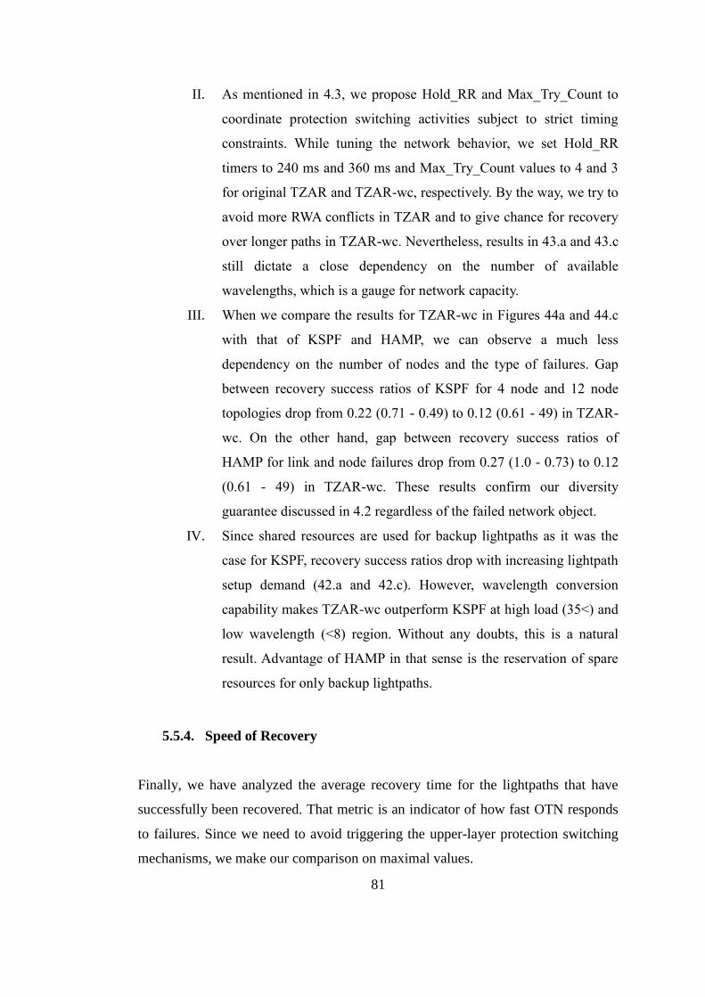
81

II. As mentioned in 4.3, we propose Hold_RR and Max_Try_Count to

coordinate protection switching activities subject to strict timing

constraints. While tuning the network behavior, we set Hold_RR

timers to 240 ms and 360 ms and Max_Try_Count values to 4 and 3

for original TZAR and TZAR-wc, respectively. By the way, we try to

avoid more RWA conflicts in TZAR and to give chance for recovery

over longer paths in TZAR-wc. Nevertheless, results in 43.a and 43.c

still dictate a close dependency on the number of available

wavelengths, which is a gauge for network capacity.

III. When we compare the results for TZAR-wc in Figures 44a and 44.c

with that of KSPF and HAMP, we can observe a much less

dependency on the number of nodes and the type of failures. Gap

between recovery success ratios of KSPF for 4 node and 12 node

topologies drop from 0.22 (0.71 - 0.49) to 0.12 (0.61 - 49) in TZAR-

wc. On the other hand, gap between recovery success ratios of

HAMP for link and node failures drop from 0.27 (1.0 - 0.73) to 0.12

(0.61 - 49) in TZAR-wc. These results confirm our diversity

guarantee discussed in 4.2 regardless of the failed network object.

IV. Since shared resources are used for backup lightpaths as it was the

case for KSPF, recovery success ratios drop with increasing lightpath

setup demand (42.a and 42.c). However, wavelength conversion

capability makes TZAR-wc outperform KSPF at high load (35<) and

low wavelength (<8) region. Without any doubts, this is a natural

result. Advantage of HAMP in that sense is the reservation of spare

resources for only backup lightpaths.

5.5.4. Speed of Recovery

Finally, we have analyzed the average recovery time for the lightpaths that have

successfully been recovered. That metric is an indicator of how fast OTN responds

to failures. Since we need to avoid triggering the upper-layer protection switching

mechanisms, we make our comparison on maximal values.

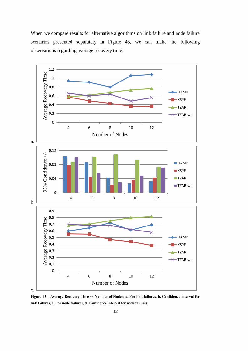
82

When we compare results for alternative algorithms on link failure and node failure

scenarios presented separately in Figure 45, we can make the following

observations regarding average recovery time:

a.

b.

c.

Figure 45 – Average Recovery Time vs Number of Nodes: a. For link failures, b. Confidence interval for


0

0,2

0,4

0,6

0,8

1

1,2

4 6 8 10 12

Aver

age

Rec

over

y T

ime

Number of Nodes

HAMP

KSPF

TZAR

TZAR-wc

0

0,04

0,08

0,12

4 6 8 10 12

95%

Confi

den

ce +

/-

HAMP

KSPF

TZAR

TZAR-wc

0

0,1

0,2

0,3

0,4

0,5

0,6

0,7

0,8

0,9

4 6 8 10 12

Aver

age

Rec

over

y T

ime

Number of Nodes

HAMP

KSPF

TZAR

TZAR-wc

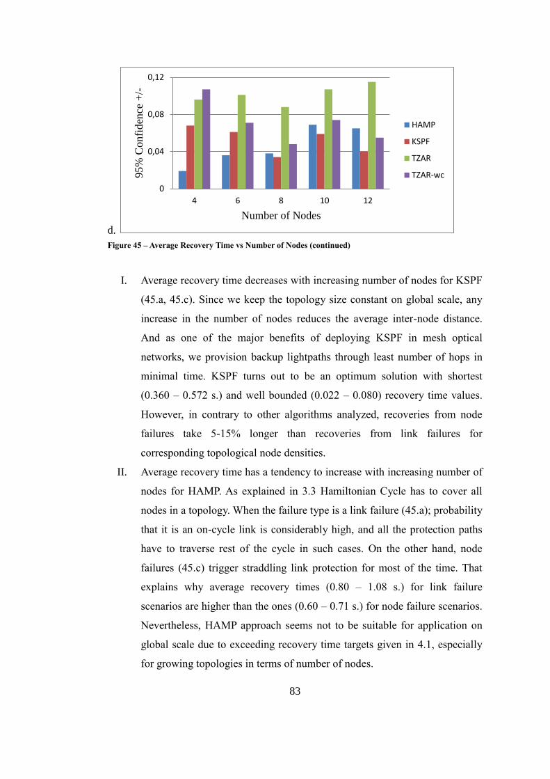
83

d.

Figure 45 – Average Recovery Time vs Number of Nodes (continued)

I. Average recovery time decreases with increasing number of nodes for KSPF

(45.a, 45.c). Since we keep the topology size constant on global scale, any

increase in the number of nodes reduces the average inter-node distance.

And as one of the major benefits of deploying KSPF in mesh optical

networks, we provision backup lightpaths through least number of hops in

minimal time. KSPF turns out to be an optimum solution with shortest

(0.360 – 0.572 s.) and well bounded (0.022 – 0.080) recovery time values.

However, in contrary to other algorithms analyzed, recoveries from node

failures take 5-15% longer than recoveries from link failures for

corresponding topological node densities.

II. Average recovery time has a tendency to increase with increasing number of

nodes for HAMP. As explained in 3.3 Hamiltonian Cycle has to cover all

nodes in a topology. When the failure type is a link failure (45.a); probability

that it is an on-cycle link is considerably high, and all the protection paths

have to traverse rest of the cycle in such cases. On the other hand, node

failures (45.c) trigger straddling link protection for most of the time. That

explains why average recovery times (0.80 – 1.08 s.) for link failure

scenarios are higher than the ones (0.60 – 0.71 s.) for node failure scenarios.

Nevertheless, HAMP approach seems not to be suitable for application on

global scale due to exceeding recovery time targets given in 4.1, especially

for growing topologies in terms of number of nodes.

0

0,04

0,08

0,12

4 6 8 10 12

95%

Confi

den

ce +

/-

Number of Nodes

HAMP

KSPF

TZAR

TZAR-wc

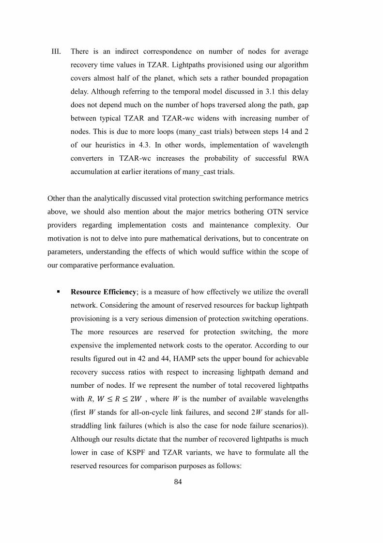
84

III. There is an indirect correspondence on number of nodes for average

recovery time values in TZAR. Lightpaths provisioned using our algorithm

covers almost half of the planet, which sets a rather bounded propagation

delay. Although referring to the temporal model discussed in 3.1 this delay

does not depend much on the number of hops traversed along the path, gap

between typical TZAR and TZAR-wc widens with increasing number of

nodes. This is due to more loops (many_cast trials) between steps 14 and 2

of our heuristics in 4.3. In other words, implementation of wavelength

converters in TZAR-wc increases the probability of successful RWA

accumulation at earlier iterations of many_cast trials.

Other than the analytically discussed vital protection switching performance metrics

above, we should also mention about the major metrics bothering OTN service

providers regarding implementation costs and maintenance complexity. Our

motivation is not to delve into pure mathematical derivations, but to concentrate on

parameters, understanding the effects of which would suffice within the scope of

our comparative performance evaluation.

Resource Efficiency; is a measure of how effectively we utilize the overall

network. Considering the amount of reserved resources for backup lightpath

provisioning is a very serious dimension of protection switching operations.

The more resources are reserved for protection switching, the more

expensive the implemented network costs to the operator. According to our

results figured out in 42 and 44, HAMP sets the upper bound for achievable

recovery success ratios with respect to increasing lightpath demand and

number of nodes. If we represent the number of total recovered lightpaths

with R, , where W is the number of available wavelengths

(first W stands for all-on-cycle link failures, and second 2W stands for all-

straddling link failures (which is also the case for node failure scenarios)).

Although our results dictate that the number of recovered lightpaths is much

lower in case of KSPF and TZAR variants, we have to formulate all the

reserved resources for comparison purposes as follows:

85

i. HAMP consumes 𝐶 = × (wavelength-link products), where C

stands for protection cost and N stands for the number of nodes.

Regardless of the number of lightpaths to be recovered, that much

resource is allocated for the Hamiltonian p-Cycle.

ii. KSPF consumes 𝐶 = × (wavelength-link products), where P

stands for average path length of backup lightpaths. According to a

detailed analysis in [73]; ≅ ln ln ⁄ , where D stands for the

average degree of nodes. Since in our OTN domain we consider nodal

degrees of 3 to 6, range for C is subject to ln 8⁄ ln ⁄ .

When we use the expression above relating R to W, even the upper

bound for protection cost of KSPF turns out to be much smaller than

the lower bound for that of HAMP for increasing number of nodes:

× ln ⁄ × .

iii. TZAR and TZAR-wc not only traverse longer backup lightpaths when

compared to KSPF, but also consume transient resources on

many_cast phase. However even for the largest possible P, i.e.

ln 7⁄ ( = ), protection cost still stays slightly worse than KSPF

but much better than HAMP.

Computation Complexity; is a measure of how difficult it is to manage the

protection switching framework. Rather than the space complexity, we do

care about time complexity due to the strict timing constraints.

i. KSPF finds k-shortest paths from a given source to any other node in

the network within 𝑂 + log + time [74], where m is

number of links, n is number of nodes, and k is the number of paths to

be found.

ii. Complexity of Hamiltonian Cycle Problem has evolved from 𝑂 ! to

𝑂 3 using brute force search and divide-and-conquer methods,

respectively. But it is also possible to construct 4-connected planar

networks within linear time 𝑂 . [75]

iii. TZAR and TZAR-wc do not introduce any algorithmic depth other

than the complexity of enumeration of neighboring nodes, which stays

in 𝑂 .

86

With the enlightenment of simulation results that we have discussed so far, we can

summarize our understanding about the key benefits of each algorithm as given in

Table 9. Although KSPF seems to be the champion in most of the metrics, its

computation complexity is an important barrier to be surmounted. HAMP suffers

badly from the dominance of very high propagation delays on intercontinental links.

TZAR, on the other hand, has to wait for cheaper and finer-tunable wavelength

converters to be considered again.

Table 9 – Protection Switching Algorithm Comparison

KSPF HAMP TZAR TZAR-wc

Recovery Success Ratio Moderate High Low Moderate

Speed of Recovery High Low Moderate Moderate

Resource Efficiency High Low Moderate Moderate

Computation Complexity High Moderate Low Low

87

CHAPTER 6

CONCLUSION

In this thesis, we first provide a brief overview of progress in optical transport

networking from hardware architecture and software hierarchy points of views

together with trends in protection switching through a peculiar taxonomy on

computational, topological, and efficiency aspects. We then propose a new low

computation complexity algorithm, TZAR, and its variety with wavelength

conversion support, TZAR-wc. These algorithms fulfill the following requirements

as expected in Appendix A based on time-zone awareness of OTN nodes:

A.1, A.2, A.3, A.10, A.20, A.24; by utilizing the existing OOS channel for

signaling and OTM hierarchy for encapsulation.

A.4, A.23; by employing carrier and domain independent time-zone

parameter as a cross-layer information.

A.5, A.6, A.7, A.25, A.26; by using SF, RR messages on a granular basis on

the levels of both lightpath clients and communicating nodes.

A.11, A.12, A.14; by managing timers like Hold_RR and counters like

Max_Try_Count.

A.16, A.19; by keeping track of candidate interfaces and featuring

Many_Cast operation.

Our detailed comparative analysis of TZAR/TZAR-wc show that we achieve 𝑂

computational complexity while KSPF and HAMP algorithms have complexities

that increase with the number of nodes and links in the topology. However, the

simple implementation of TZAR/TZAR-wc cannot achieve the best values in

88

Recovery Success Ratio, Speed of Recovery and Resource Efficiency metrics

compared to KSPF and HAMP.

Furthermore, our results show that in the presence of wavelength conversion

capability, the quasi-ring decomposition of global mesh topologies is a sound

routing alternative to be investigated further in literature. Meanwhile, “Time Zone”

parameter may probably be the most natural argument to support the deployment of

TZAR sort of approaches in next generation OTN systems. Though wavelength

converters act as a key enabler to obtain new recovery success ratios, average

number of wavelength converters on each node would be of concern.

In this study we have primarily focused on failure recovery framework in OTN. As

future work one can suggest, investigating revertive mode of operation with

wavelength conversion to evaluate how network behaves when failed resources

come back into their initial working states. Consequently, expectations A.15 and

A.22 would be satisfied. Once lightpath allocation and de-allocation mechanisms

are defined, prioritization and preemption procedures can also be specified in a

straightforward manner. By the way, expectations A.17 and A.21 could be satisfied.

Utilizing a tighter integration with control and management planes might produce

enough capabilities to monitor the real time status of transport plane. Satisfaction of

expectations A.8, A.9, A.13, and A.18 would then follow to avoid contention for the

shared resources while keeping sharing gain at reasonable levels.

To sum up, autonomous protection switching for failed lightpaths will continue to

be a sophisticated traffic recovery framework demand especially when used in

conjunction with BGP and GMPLS sort of upper layer protocols. Since most of

Tier-1 ISPs running BGP has presence in multiple IXP sites and global CDN

operators lease resources to be managed privately by GMPLS, global resilience on

mesh OTN is of utmost interest in the nearest term. With its indeterminate nature

TZAR would not be appropriate as a primary solution, but its adjustable behavior

may address TZAR as a real-time backup for KSPF or HAMP sort of protection

switching algorithms.

89

REFERENCES

[1] Alcatel-Lucent, “Alcatel-Lucent to double capacity of today’s data transport

networks by being first to deliver a single-carrier 200G DWDM optical line card”

“http://www.alcatel-lucent.com/press/2014/alcatel-lucent-double-capacity-todays-

data-transport-networks-being-first-deliver-single-carrier”, 24 September 2014

[2] ITU-T Recommendation G.696.1, “Longitudinally compatible intra-domain

DWDM applications”, Telecommunication Standardization Sector of ITU, July

2010

[3] Yoichi Maeda, Francesco Montalti, Gastone Bonaventura, Makoto Murakami,

and Kazuyuki Shiraki, “Optical fibre, cables and systems”, ITU-T Manual, 2009

[4] Infinera Corporation, “Infinera Customers Deploy over one Petabit per second

of Super-Channel Transmission Capacity Globally”,

“http://www.infinera.com/j7/servlet/NewsItem?newsItemID=395”, 27 March 2014

[5] “The Zettabyte Era: Trends and Analysis”, Cisco, 10 June 2014

[6] Andrew Schmitt, “Global Service Provider Survey Excerpts: OTN, MPLS, and

Control Plane Strategies”, Infonetics Research, Inc., June 2013

[7] Michael Ruddy on behalf of Terabit Consulting, “Submarine Telecoms Industry

Report”, Submarine Telecoms Forum, 2014

[8] Ron Kline, “Vendor strategies: Tellabs fights back against larger full-service

rivals”, Ovum, 16 June 2010

[9] “TrueNet Capabilities Overview”, ADC Telecommunications, Inc., 2009

http://www.alcatel-lucent.com/press/2014/alcatel-lucent-double-capacity-todays-data-transport-networks-being-first-deliver-single-carrier

http://www.alcatel-lucent.com/press/2014/alcatel-lucent-double-capacity-todays-data-transport-networks-being-first-deliver-single-carrier

http://www.infinera.com/j7/servlet/NewsItem?newsItemID=395

90

[10] James P.G. Sterbenz, David Hutchison, Egemen K. Çetinkaya, Abdul Jabbar,

Justin P. Rohrer, Marcus Schöller, Paul Smith, “Resilience and survivability in

communication networks: Strategies, principles, and survey of disciplines”, Elsevier

- Computer Networks, 2010

[11] ITU-T Recommendation G.709/Y.1331, “Interfaces for the optical transport

network”, Telecommunication Standardization Sector of ITU, February 2012

[12] ITU-T Recommendation G.872, “Architecture of optical transport networks”,

Telecommunication Standardization Sector of ITU, October 2012

[13] ITU-T Recommendation G.798, “Characteristics of optical transport network

hierarchy equipment functional blocks”, Telecommunication Standardization Sector

of ITU, December 2012

[14] Paul Littlewood, Fady Masoud, “Optical Transport Networking”, Ciena Expert

Series, 2014

[15] Steve Gorshe, “A Tutorial on ITU-T G.709 Optical Transport Networks

(OTN)”, PMC-Sierra, Inc., June 2011

[16] Richard A Steenbergen, “Everything You Always Wanted to Know About

Optical Networking – But Were Afraid to Ask”, NANOG Meeting 57, February

2013

[17] Emmanuel Desurvire, “Erbium-doped fiber amplifiers: device and system

developments”, J. Wiley & Sons, 2002

[18] Mahmud Wasfi, “Optical Fiber Amplifiers-Review”, International Journal of

Communication Networks and Information Security (IJCNIS), April 2009

[19] ITU-T Recommendation G.694.2, “Spectral grids for WDM applications:

CWDM wavelength grid”, Telecommunication Standardization Sector of ITU,

December 2003

91

[20] ITU-T Recommendation G.694.1, “Spectral grids for WDM applications:

DWDM frequency grid”, Telecommunication Standardization Sector of ITU,

February 2012

[21] Dhritiman Banerjee, Biswanath Mukherjee, “A Practical Approach for Routing

and Wavelength Assignment in Large Wavelength-Routed Optical Networks”,

IEEE Journal on Selected Areas in Communications, June 1996

[22] Rajiv Ramaswami, Kumar N. Sivarajan, “Routing and Wavelength Assignment

in All-Optical Networks”, IEEE/ACM Transactions on Networking, October 1995

[23] Matthieu Clouqueur, Wayne D. Grover, “Availability Analysis of Span-

Restorable Mesh Networks”, IEEE Journal on Selected Areas in Communications,

May 2002

[24] Richard A. Barry, Pierre A. Humblet, “Models of Blocking Probability in All-

Optical Networks with and without Wavelength Changers”, IEEE Journal on

Selected Areas in Communications, June 1996

[25] Byrav Ramamurthy, Biswanath Mukherjee, “Wavelength Conversion in

WDM Networking”, IEEE Journal on Selected Areas in Communications,

September 1998

[26] I. Chlamtac, A. Ganz, G. Karmi, “Lightpath communications: an approach to

high bandwidth optical WAN's”, IEEE Transactions on Communications, July 1992

[27] Rajiv Ramaswami, “Optical Networking Technologies: What Worked and

What Didn't”, IEEE Communications Magazine, September 2006

[28] Mohcene Mezhoudi, Chi-Hung Kelvin Chu, “Integrating Optical Transport

Quality, Availability, and Cost Through Reliability-Based Optical Network

Design”, Bell Labs Technical Journal, May 2006

[29] Laxman Sahasrabuddhe, S. Ramamurthy, Biswanath Mukherjee, “Fault

Management in IP-Over-WDM Networks: WDM Protection Versus IP

Restoration”, IEEE Journal on Selected Areas in Communications, January 2002

92

[30] ITU-T Recommendation G.8080/Y.1304, “Architecture for the automatically

switched optical network”, Telecommunication Standardization Sector of ITU,

February 2012

[31] ITU-T Recommendation G.808.1, “Generic protection switching – Linear trail

and subnetwork protection”, Telecommunication Standardization Sector of ITU,

May 2014

[32] ITU-T Recommendation G.808.2, “Generic protection switching – Ring

protection”, Telecommunication Standardization Sector of ITU, November 2013

[33] ITU-T Recommendation G.808.3, “Generic protection switching – Shared

mesh protection”, Telecommunication Standardization Sector of ITU, October 2012

[34] Eric Bouillet, Georgios Ellinas, Jean-François Labourdette, Ramu

Ramamurthy, “Path Routing in Mesh Optical Networks”, John Wiley & Sons, 2007

[35] Nico Wauters, Gzim Ocakoglu, Kris Struyve, Pedro Falcao Fonseca,

“Survivability in a New Pan-European Carriers’ Carrier Network Based on WDM

and SDH Technology: Current Implementation and Future Requirements”, IEEE

Communications Magazine, August 1999

[36] Hamza Drid, Bernard Cousin, Miklos Molnar, Samer Lahoud, “A survey of

survivability in multi-domain optical networks”, Elsevier - Computer

Communications, February 2010

[37] Mohit Chamania, Admela Jukan, “A Survey of Inter-Domain Peering and

Provisioning Solutions for the Next Generation Optical Networks”, IEEE

Communications Surveys & Tutorials, 2009

[38] ITU-T Recommendation G.873.1, “Optical transport network (OTN): Linear

protection”, Telecommunication Standardization Sector of ITU, May 2014

[39] Timothy Y. Chow, Fabian Chudak, Anthony M. Ffrench, “Fast optical layer

mesh protection using pre-cross-connected trails”, IEEE/ACM Transactions on

Networking, June 2004

93

[40] John Strand, Angela L. Chiu and Robert Tkach, “Issues For Routing In The

Optical Layer”, IEEE Communications Magazine, February 2001

[41] Hui Zang, Member, Canhui (Sam) Ou, Biswanath Mukherjee, “Path-Protection

Routing and Wavelength Assignment (RWA) in WDM Mesh Networks Under

Duct-Layer Constraints”, IEEE/ACM Transactions on Networking, April 2003

[42] Lei Song, Biswanath Mukherjee, “On The Study of Multiple Backups and

Primary-Backup Link Sharing for Dynamic Service Provisioning in Survivable

WDM Mesh Networks”, IEEE Journal on Selected Areas in Communications, 2008

[43] Dongyun Zhou, Suresh Subramaniam, “Survivability in Optical Networks”,

IEEE Network, November/December 2000

[44] János Tapolcai, Pin-Han Ho, Péter Babarczi, Lajos Rónyai, “Internet Optical

Infrastructure: Issues on Monitoring and Failure Restoration”, Springer, 2015

[45] J. Y. Yen, “Finding the K shortest loopless paths in a network”, Journal of

Management Science, July 1971

[46] J. W. Suurballe, “Disjoint paths in a network”, Networks, 1974

[47] J. Rak, “k-Penalty: a novel approach to find k-Disjoint paths with differentiated

path costs”, IEEE Communication Letters, April 2010

[48] P. Merindol, “An efficient algorithm to enable path diversity in link state

routing networks”, Elsevier – Computer Networks, 2011

[49] Dominic A. Schupke, “Automatic protection switching for p-cycles in WDM

networks”, Elsevier – Optical Switching and Networking, April 2005

[50] Ramin Saeedinia, “Protection Switching in Communication Networks”, IEEE

UKRI – 16th

European Conference on Networks and Optical Communications, 2011

[51] Mohammad S. Kiaei, Chadi Assi, and Brigitte Jaumard, “A Survey on the p-

Cycle Protection Method”, IEEE Communications Surveys & Tutorials, 2009

94

[52] Wayne D. Grover, Demetrios Stamatelakis, “Cycle-Oriented Distributed

Preconfiguration: Ring-like Speed with Mesh-like Capacity for Self-planning

Network Restoration”, IEEE, 1998

[53] Hong Huang, John Copeland, “Hamiltonian Cycle Protection: A Novel

Approach to Mesh WDM Optical Network Protection”, IEEE, 2001

[54] John Doucette1, Peter A. Giese1, Wayne D. Grover, “Combined Node and

Span Protection Strategies with Node-Encircling p-Cycles”, IEEE, 2005

[55] Adil Kodian, Wayne D. Grover, “Failure-Independent Path-Protecting p-

Cycles: Efficient and Simple Fully Preconnected Optical-Path Protection”, Journal

of Lightwave Technology, October 2005

[56] ITU-T Recommendation G.841, “Types and characteristics of SDH network

protection architectures”, Telecommunication Standardization Sector of ITU,

October 1998

[57] ITU-T Recommendation G.8031/Y.1342, “Ethernet linear protection

switching”, Telecommunication Standardization Sector of ITU, January 2015

[58] The Solutions Center, “Solution Guide: SAN Distance Extension Reference”,

Brocade Communications Systems, 2007

[59] Tom Scholl, “BFD (Bidirectional Forwarding Detection) Does it work and is it

worth it?”, NANOG Meeting 45, January 2009

[60] Dimitri Staessens, Didier Colle, Ilse Lievens, Mario Pickavet, Piet Demeester,

Walter Colitti, Ann Nowé, Kris Steenhaut, Ricardo Romeral, “Enabling High

Availability over Multiple Optical Networks”, IEEE Communications Magazine,

June 2008

[61] Stephanie Silvius, “Internet Exchange Points”, European Internet Exchange

Association Reports, January 2011

95

[62] Chengchen Hu, Kai Chen, Yan Chen, Bin Liu, Athanasios V. Vasilakos, “A

Measurement Study on Potential Inter-Domain Routing Diversity”, IEEE

Transactions on Network and Service Management, September 2012

[63] Packet Clearing House, https://prefix.pch.net/applications/ixpdir/, May 2015

[64] Melanie Posey, “Is Your Application Delivery Approach Optimized to Meet

the Needs of Your Globally Distributed User Base?”, International Data

Corporation (IDC), December 2014

[65] Amy Cravens, “How new devices, networks, and consumer habits will change

the web experience”, GigaOM Pro, January 2013

[66] Eytan Modiano, Aradhana Narula-Tam, “Survivable Lightpath Routing: A

New Approach to the Design of WDM-Based Networks”, IEEE Journal on Selected

Areas in Communications, 2002

[67] C. E. Perkins, E. M. Belding-Royer, S. R. Das, “Ad hoc On-Demand Distance

Vector (AODV) Routing”, IETF RFC 3561, July 2003

[68] OPNET Modeler 14.5.A PL8 – Educational Version, © 1986-2008 OPNET

Technologies, Inc.1

[69] Zheng Lu, Hongji Yang, “Unlocking the Power of OPNET Modeler”,

Cambridge University Press, 2012

[70] Francesca Bontempi, Stefano Faralli, Nicola Andriolli, Giampiero

Contestabile, “An InP Monolithically Integrated Unicast and Multicast Wavelength

Converter”, IEEE Photonics Technology Letters, November 2013

[71] Dimitrios Fitsios, Theonitsa Alexoudi, George T. Kanellos, Konstantinos

Vyrsokinos, Nikos Pleros, Tolga Tekin, Matteo Cherchi, Sami Ylinen, Mikko

1 OPNET Technologies, Inc. was acquired by Riverbed in October 2012. Since then OPNET

Modeler is called Riverbed Modeler, and now a part of SteelCentral performance management

and control product portfolio.

https://prefix.pch.net/applications/ixpdir/

96

Harjanne, Markku Kapulainen, Timo Aalto, “Dual SOA-MZI Wavelength

Converters Based on III-V Hybrid Integration on a μm-Scale Si Platform”, IEEE

Photonics Technology Letters, March 2014

[72] Houman Rastegarfar, Alberto Leon-Garcia, Sophie LaRochelle, Leslie Ann

Rusch, “Cross-Layer Performance Analysis of Recirculation Buffers for Optical

Data Centers”, IEEE Journal of Lightwave Technology, February 2013

[73] P. Erdös, A. Renyi, “On the evolution of random graphs”, Publications of the

Mathematical Institute of the Hungarian Academy of Sciences 5, 1960

[74] David Eppstein, “Finding k Shortest Paths”, Department of Information and

Computer Science, University of California, Irvine, CA, 1997

[75] Norishige Chiba, Takao Nishizeki, “The Hamiltonian Cycle Problem Is Linear-

Time Solvable for 4-Connected Planar Graphs”, Journal of Algorithms 10,

Academic Press, 1989

97

APPENDIX A

PROTECTION SWITCHING REQUIREMENTS

Generic protection switching requirements for shared mesh networks given in [22];

A.1 Shall allow backwards compatibility with core structures/formats of

technology-specific Recommendations.

A.2 Shall not impact usage of existing technology-specific linear and ring APS

protection mechanisms and communications channels (i.e., co-existence with

existing APS specifications).

A.3 Shall allow for any intra-/inter-operator applications for cascaded or nested

protection deployments.

A.4 Shall allow for co-existence of ASON-based protection/restoration and SMP

protection at inter-domain boundaries.

A.5 Shall be capable of supporting protection of one or more point-to-point

bidirectional normal traffic signals from the ingress to the egress of the SMP

domain.

A.6 Shall not require that multiple working transport entities sharing the same

protection resource(s) have the same end points.

A.7 Shall monitor the status of the working transport entities for SMP protection

switching triggers (e.g., SF, SD).

A.8 Shall monitor availability of the shared protection resources along the

protection transport entities.

98

A.9 Shall include support for communicating information on the availability of the

shared protection resources along the protection transport entities to the end points

of the working transport entities that utilize the resources.

A.10 Shall include support for communicating information among network nodes to

perform protection switching. The message encoding and communicating channel

between the nodes depends on the specific technology.

A.11 Shall be capable of recovering a normal traffic signal from network failure(s)

in a deterministic manner. For example, the protection switching shall complete

within a finite (bounded) time, as described within the technology-specific

Recommendations.

A.12 Shall include support for a mechanism to detect protocol failures.

A.13 Shall include support for a mechanism to detect possible inconsistencies in

configuration between the ingress and egress nodes of an SMP domain.

A.14 Shall be capable of supporting nesting of multiple levels of protection

(whether SMP or other schemes such as SNC protection). To achieve this, shall

include support for mechanism(s) that allow for coordination of protection activities

(e.g., hold-off timer).

A.15 Shall provide a mechanism to avoid protection switching flapping (e.g., wait-

to-restore timer).

A.16 Shall include support for multiple links between nodes, allowing for link and

node diversity, and should be scalable with respect to the number of links and nodes

within the SMP protection domain.

A.17 Shall provide a contention resolution mechanism for permitting only one

working transport entity to occupy protection resources in the case that these

protection resources are shared by more than one working transport entity having

the same priority (due to network topology and resource limitations).

99

A.18 Shall be capable of supporting the ability to set an upper limit on the

maximum number of working transport entities that can share protection resources

(which is governed by the specific technology).

A.19 Shall include support for the ability to set an upper bound on the fraction of

link resources that can be allocated to protecting transport entities.

A.20 Shall allow for configuration (which may be via the management or control

plane) of the protection transport entity identifiers, required bandwidth, and

additionally for circuit SMP, the assignment of TSs to ensure the proper operation

of the protection switching process.

A.21 Shall support assignment of priority to support the request of a higher-priority

transport entity to pre-empt the shared protection resource taken by a lower-priority

transport entity.

A.22 Shall only support revertive operation type.

A.23 Shall only support bidirectional switching type.

A.24 Shall be capable of supporting external commands from network operators.

A.25 Shall be capable of supporting protection for more than one failure, including

failures that are concurrent and/or failures involving shared resources.

A.26 Shall be capable of protection switching activation initiated by either end or

both ends (which may be simultaneous) of the SMP domain.

100

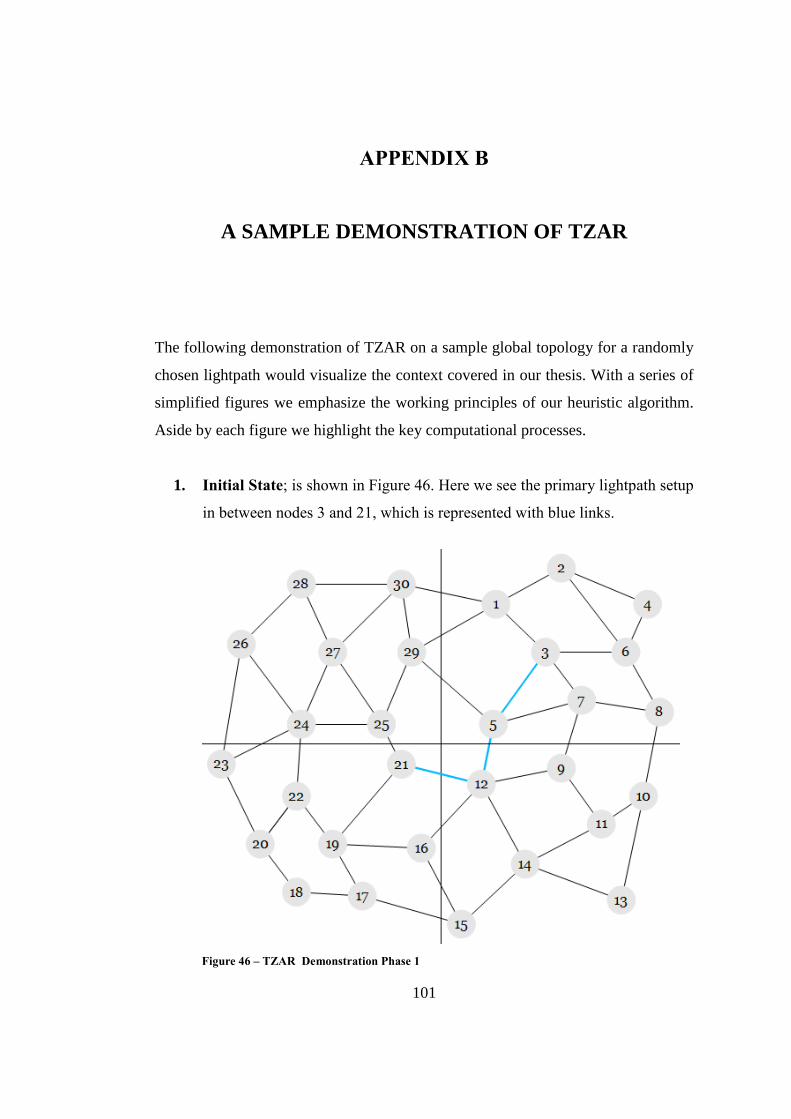
101

APPENDIX B

A SAMPLE DEMONSTRATION OF TZAR

The following demonstration of TZAR on a sample global topology for a randomly

chosen lightpath would visualize the context covered in our thesis. With a series of

simplified figures we emphasize the working principles of our heuristic algorithm.

Aside by each figure we highlight the key computational processes.

1. Initial State; is shown in Figure 46. Here we see the primary lightpath setup

in between nodes 3 and 21, which is represented with blue links.

Figure 46 – TZAR Demonstration Phase 1

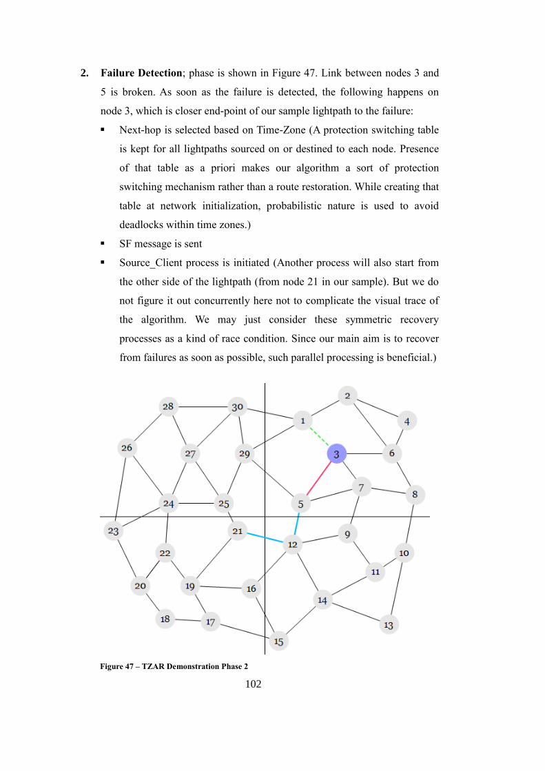
102

2. Failure Detection; phase is shown in Figure 47. Link between nodes 3 and

5 is broken. As soon as the failure is detected, the following happens on

node 3, which is closer end-point of our sample lightpath to the failure:

Next-hop is selected based on Time-Zone (A protection switching table

is kept for all lightpaths sourced on or destined to each node. Presence

of that table as a priori makes our algorithm a sort of protection

switching mechanism rather than a route restoration. While creating that

table at network initialization, probabilistic nature is used to avoid

deadlocks within time zones.)

SF message is sent

Source_Client process is initiated (Another process will also start from

the other side of the lightpath (from node 21 in our sample). But we do

not figure it out concurrently here not to complicate the visual trace of

the algorithm. We may just consider these symmetric recovery

processes as a kind of race condition. Since our main aim is to recover

from failures as soon as possible, such parallel processing is beneficial.)


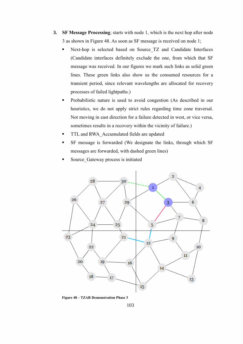
103

3. SF Message Processing; starts with node 1, which is the next hop after node

3 as shown in Figure 48. As soon as SF message is received on node 1;

Next-hop is selected based on Source_TZ and Candidate Interfaces

(Candidate interfaces definitely exclude the one, from which that SF

message was received. In our figures we mark such links as solid green

lines. These green links also show us the consumed resources for a

transient period, since relevant wavelengths are allocated for recovery

processes of failed lightpaths.)

Probabilistic nature is used to avoid congestion (As described in our

heuristics, we do not apply strict rules regarding time zone traversal.

Not moving in east direction for a failure detected in west, or vice versa,

sometimes results in a recovery within the vicinity of failure.)

TTL and RWA_Accumulated fields are updated

SF message is forwarded (We designate the links, through which SF

messages are forwarded, with dashed green lines)

Source_Gateway process is initiated


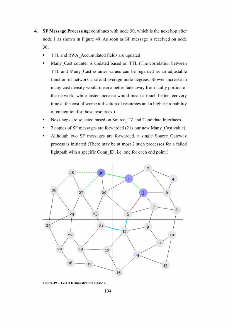
104

4. SF Message Processing; continues with node 30, which is the next hop after

node 1 as shown in Figure 49. As soon as SF message is received on node

30;


Many_Cast counter is updated based on TTL (The correlation between

TTL and Many_Cast counter values can be regarded as an adjustable

function of network size and average node degrees. Slower increase in

many-cast density would mean a better fade away from faulty portion of

the network, while faster increase would mean a much better recovery

time at the cost of worse utilization of resources and a higher probability

of contention for those resources.)

Next-hops are selected based on Source_TZ and Candidate Interfaces

2 copies of SF messages are forwarded (2 is our new Many_Cast value)

Although two SF messages are forwarded, a single Source_Gateway

process is initiated (There may be at most 2 such processes for a failed

lightpath with a specific Conn_ID, i.e. one for each end point.)


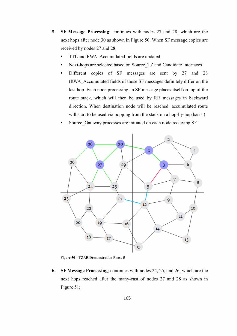
105

5. SF Message Processing; continues with nodes 27 and 28, which are the

next hops after node 30 as shown in Figure 50. When SF message copies are

received by nodes 27 and 28;


Next-hops are selected based on Source_TZ and Candidate Interfaces

Different copies of SF messages are sent by 27 and 28

(RWA_Accumulated fields of those SF messages definitely differ on the

last hop. Each node processing an SF message places itself on top of the

route stack, which will then be used by RR messages in backward

direction. When destination node will be reached, accumulated route

will start to be used via popping from the stack on a hop-by-hop basis.)

Source_Gateway processes are initiated on each node receiving SF


6. SF Message Processing; continues with nodes 24, 25, and 26, which are the

next hops reached after the many-cast of nodes 27 and 28 as shown in

Figure 51;

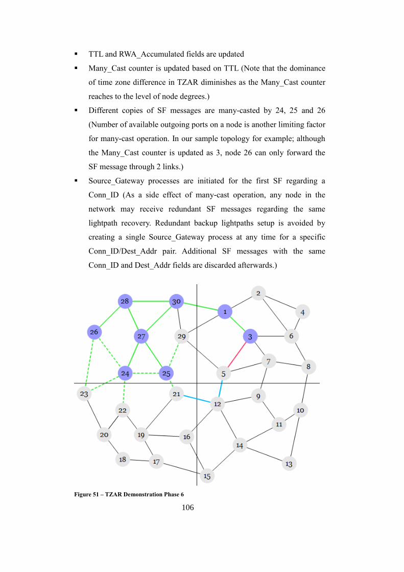
106


Many_Cast counter is updated based on TTL (Note that the dominance

of time zone difference in TZAR diminishes as the Many_Cast counter

reaches to the level of node degrees.)

Different copies of SF messages are many-casted by 24, 25 and 26

(Number of available outgoing ports on a node is another limiting factor

for many-cast operation. In our sample topology for example; although

the Many_Cast counter is updated as 3, node 26 can only forward the

SF message through 2 links.)

Source_Gateway processes are initiated for the first SF regarding a

Conn_ID (As a side effect of many-cast operation, any node in the

network may receive redundant SF messages regarding the same

lightpath recovery. Redundant backup lightpaths setup is avoided by

creating a single Source_Gateway process at any time for a specific

Conn_ID/Dest_Addr pair. Additional SF messages with the same

Conn_ID and Dest_Addr fields are discarded afterwards.)


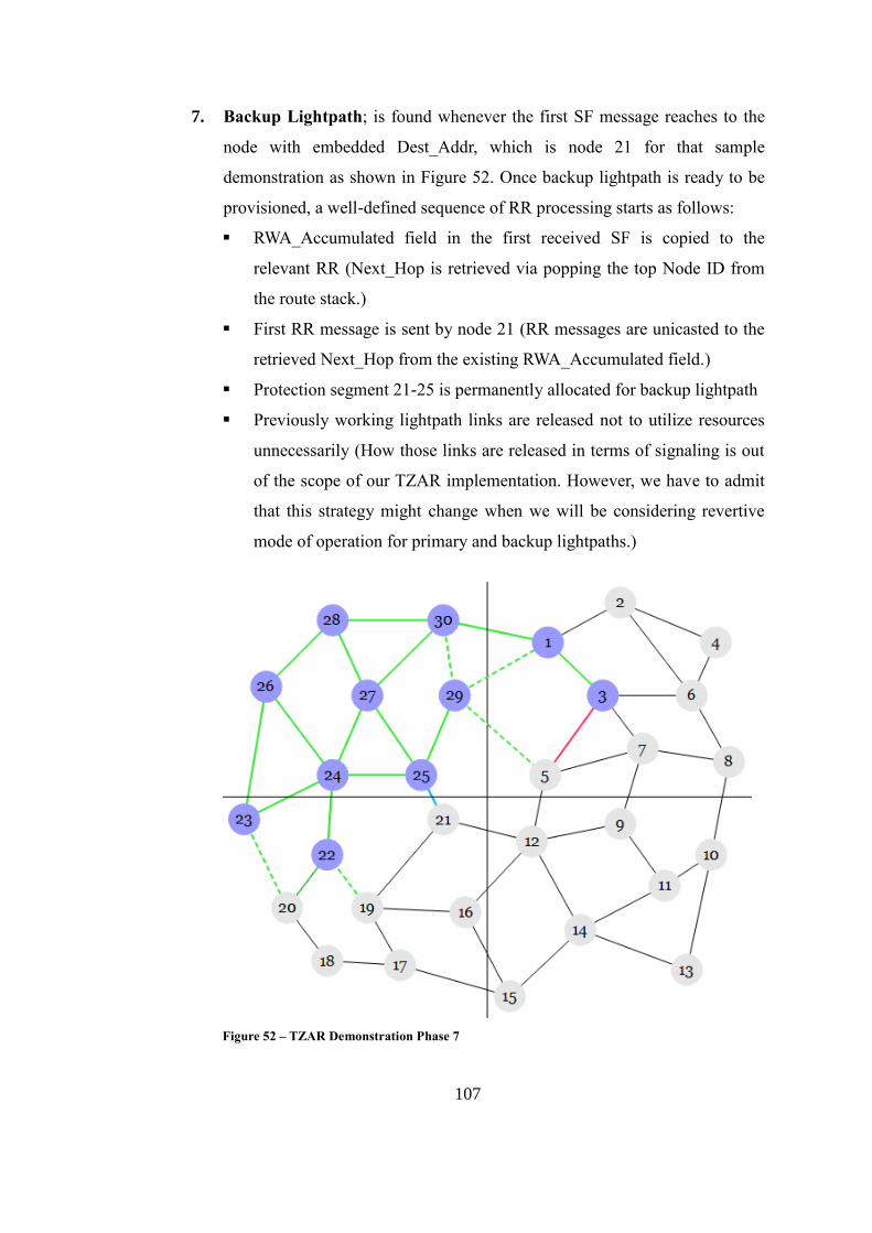
107

7. Backup Lightpath; is found whenever the first SF message reaches to the

node with embedded Dest_Addr, which is node 21 for that sample

demonstration as shown in Figure 52. Once backup lightpath is ready to be

provisioned, a well-defined sequence of RR processing starts as follows:

RWA_Accumulated field in the first received SF is copied to the

relevant RR (Next_Hop is retrieved via popping the top Node ID from

the route stack.)

First RR message is sent by node 21 (RR messages are unicasted to the

retrieved Next_Hop from the existing RWA_Accumulated field.)

Protection segment 21-25 is permanently allocated for backup lightpath

Previously working lightpath links are released not to utilize resources

unnecessarily (How those links are released in terms of signaling is out

of the scope of our TZAR implementation. However, we have to admit

that this strategy might change when we will be considering revertive

mode of operation for primary and backup lightpaths.)


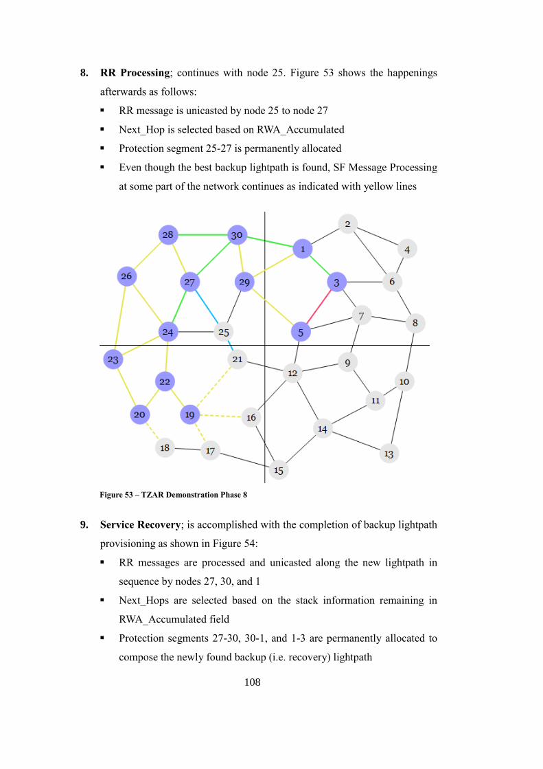
108

8. RR Processing; continues with node 25. Figure 53 shows the happenings

afterwards as follows:

RR message is unicasted by node 25 to node 27

Next_Hop is selected based on RWA_Accumulated

Protection segment 25-27 is permanently allocated

Even though the best backup lightpath is found, SF Message Processing

at some part of the network continues as indicated with yellow lines


9. Service Recovery; is accomplished with the completion of backup lightpath

provisioning as shown in Figure 54:

RR messages are processed and unicasted along the new lightpath in

sequence by nodes 27, 30, and 1

Next_Hops are selected based on the stack information remaining in

RWA_Accumulated field

Protection segments 27-30, 30-1, and 1-3 are permanently allocated to

compose the newly found backup (i.e. recovery) lightpath

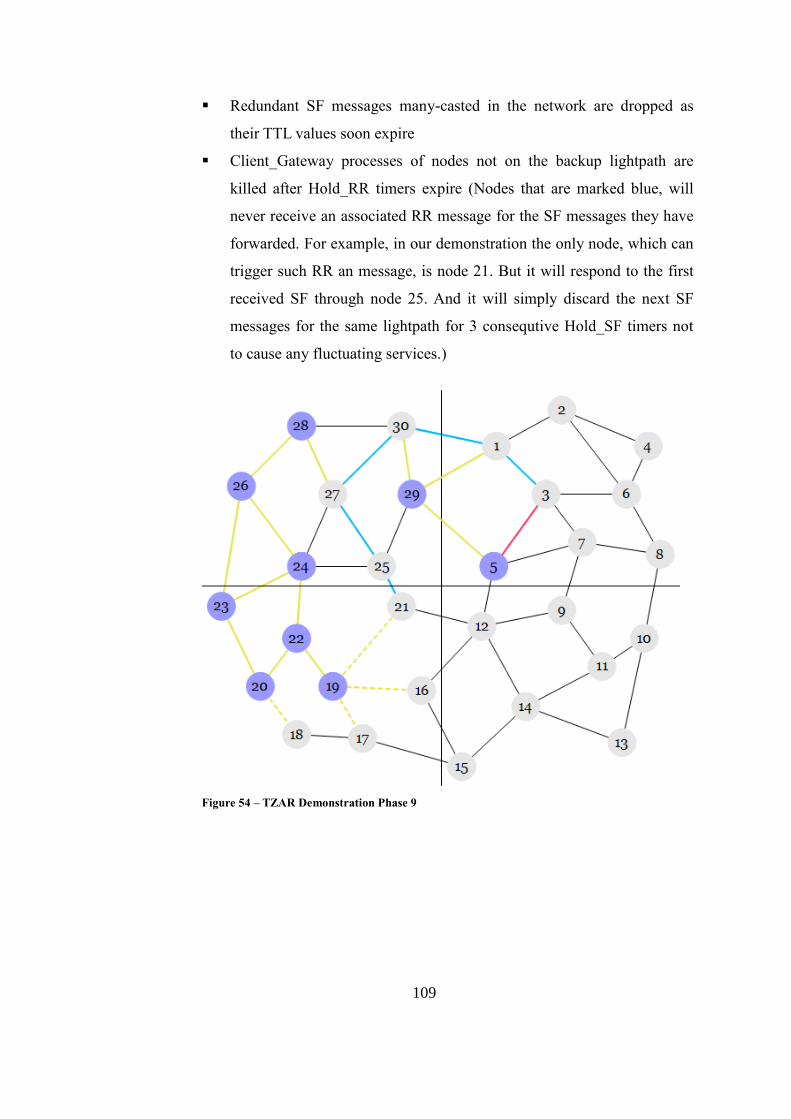
109

Redundant SF messages many-casted in the network are dropped as

their TTL values soon expire

Client_Gateway processes of nodes not on the backup lightpath are

killed after Hold_RR timers expire (Nodes that are marked blue, will

never receive an associated RR message for the SF messages they have

forwarded. For example, in our demonstration the only node, which can

trigger such RR an message, is node 21. But it will respond to the first

received SF through node 25. And it will simply discard the next SF

messages for the same lightpath for 3 consequtive Hold_SF timers not

to cause any fluctuating services.)


Documents

TZAR TIME ZONE BASED APPROXIMATION TO RING: AN …