U. S. DEPARTMENT OF COMMERCENATIONAL OCEANIC AND ATMOSPHERIC ADMINISTRATION

NATIONAL WEATHER SERVICENATIONAL METEOROLOGICAL CENTER

OFFICE NOTE 315

THE NEW NMC MEDIUM RANGE FORECAST MODEL -- AN INTRODUCTORY NOTE

JOSEPH P. GERRITY, JR., John H. WARD, AND GLENN H. WHITEMEDIUM-RANGE MODELING BRANCH

OCTOBER 1985

THIS IS AN UNREVIEWED MANUSCRIPT, PRIMARILY INTENDED FORINFORMAL EXCHANGE OF INFORMATION AMONG NMC STAFF MEMBERS.

0

THE NEW NMC MEDIUM RANGE FORECAST MODEL -- AN INTRODUCTORY NOTE

J. P. Gerrity, Jr., J. H. Ward, and G. H. White

Development Division, NMC, NWS, NOAAWashington, DC

1. Introduction

A new medium range, numerical weather prediction model was implemented at

the U.S. National Meteorological Center (NMC) on April 17, 1985. This note

provides a general introduction to the new model which is referred to as the

MRF, or medium range forecast, model.

In the summer of 1983, NMC began to use its new supercomputer, a CYBER

205. By taking advantage of the computer's capabilities for very rapid processing

of long data strings, or vectors, it was possible to increase the horizontal

resolution of the NMC global spectral model from rhomboidal 30 to rhomboidal

40 spectral truncation. The provision to NMC of authorization to use highly

optimized Fast Fourier Transforms developed by C. Temperton at the British

Meteorological Office was instrumental in.this stage of development.

Subsequent to the implemehtation ofthe rhomboidal-40 model, work was

begun to augment the sophisticatlon of the physics parameterizations used in

the model. Extensive collaboration with NOAA's Geophysical Fluid Dynamics

Laboratory (GFDL) accelerated this process. Concurrently the model's vertical

resolution was increased from 12 to 18 layers. By the Summer of 1984 a series

of test integrations with the new model were undertaken at NMC. The success

obtained, warranted an intensive daily comparison between the new model and the

operational forecast model. A number of improvements were effected during the

course of this experimental work. The last change, made in January 1985,

involved the introduction of a "silhouette orography" following a suggestion

2

of Fedor Mesinger. Comparative results for the new model and the operational

model obtained during February and March 1985, a period during which both

models remained invariant, are shown later on.

At the time of writing, the new model has been operational for just four

months. We anticipate further development of the model to achieve greater

efficiency of operation and increased accuracy of the forecasts. This pre-

sentation is limited to outlining the broad characteristics of the model and

giving a preliminary assessment of its accuracy. A complete description of

the mathematical and physical bases for the model will be prepared later.

2. General Characteristics of the MRF Model

The new medium-range forecast (MRF) model has been constructed on the

foundation of the CYBER version of the NMC global spectral model. The basic

design of that model has been described previously (Sela, 1982). In this

section, we provide an overview of the changes that have been incorporated in

the model which warrant its new appelation, MRF.

2.1 Vertical Structure - Topography

The vertical resolution of the MRF model is provided by 18 layers of

equal increments of pressure normalized by the surface pressure, which is

a function of horizontal position and time. The previous NMC model had 12

unequally spaced layers. The dominant spatial variation of surface pressure

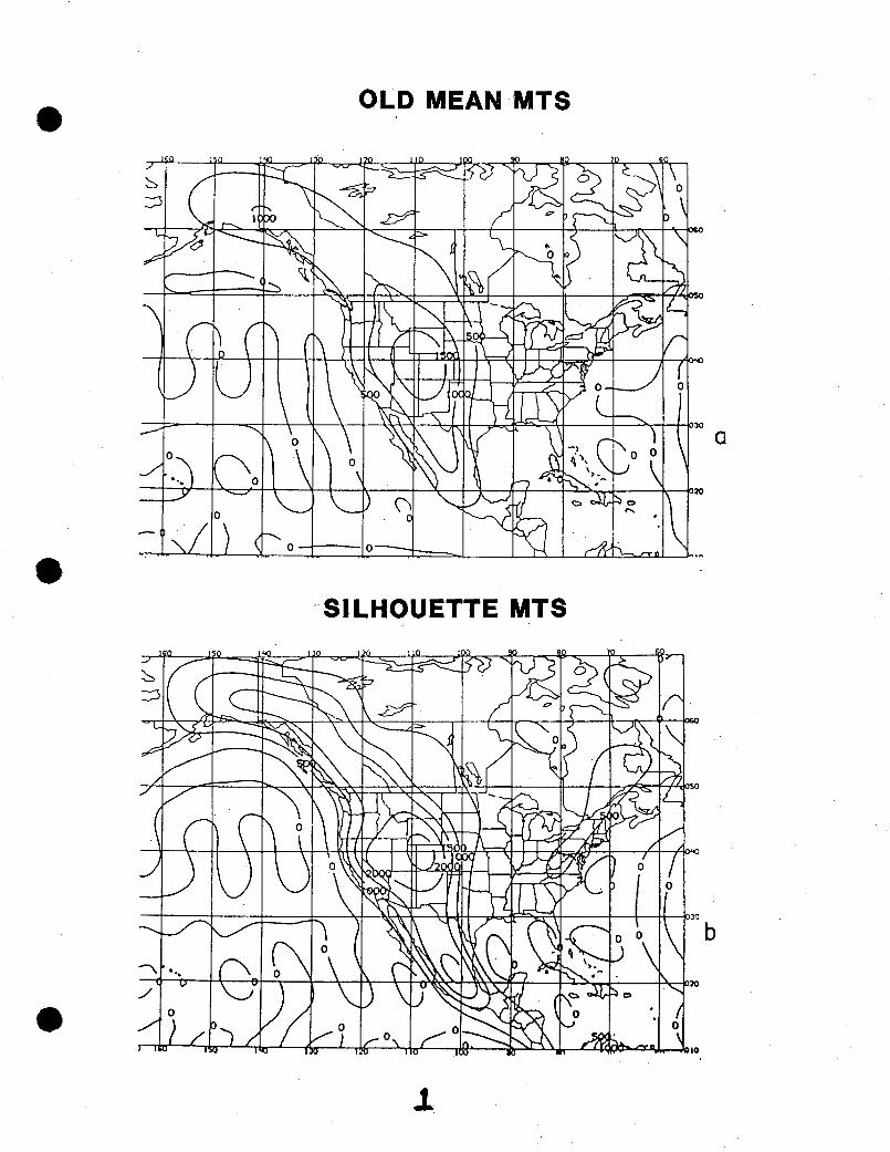
is related to the height of the model orography above mean sea level.

The field of orography was defined to reflect the silhouette of the mountains

covering each cell of the model's Gaussian grid. The new orography has appre-

ciably higher elevations than were used in the previous model. An example of

this contrast is shown in Figure l. -.

:9,- f f f 050- i' ,,: in -; A:... :.?;

3

2.2 Radiative Heat Transfer

The algorithms used for computing radiative heat transfer were provided by

GFDL where they were developed by S. Fels and D. Schwarzkopf. Because these

algorithms were designed for use with the GFDL eighteen layer model, which has

unequal layer depths, it has been necessary to interpolate the MRF's dependent

variables into the GFDL model coordinate system in order to use the algorithms.

Conversely the radiative heating rates must be interpolated from the GFDL

model's vertical coordinate into the MRF coordinate.

As presently used, the radiative heating field is recomputed at twelve

hour intervals and held constant during the intervening time period. The

algorithms account for water vapor, carbon dioxide, ozone and cloudiness. The

carbon dioxide concentration distribution is invariant. Between the surface

and approximately 300 mb water vapor is obtained from the forecast humidity

field. At higher levels, the water vapor distribution is obtained by inter-

polation between a constant value at 50 nb and the predicted value at 300 mb.

The fractional cloud cover is defined from climatological normals in three

altitude categories. The cloud field is zonally symmetric and independent of

the forecast model's water vapor and temperature fields. Ozone is also speci-

fied from climatological fields. The albedo of the underlying surface is set

to a climatological background field and is modified to reflect the distribu-

tion of snow and ice diagnosed from analysis fields, or in the case of snow

from model predictions of precipitation in sufficiently cold air.

2.3 Surface Parameterization

The surface of the earth is allowed to interact with the atmosphere over

both land and sea. Over the seas, the sea surface temperature is held invariant

at the initial values obtained from near real time analyses of ship and satellite

data. An exception is made when sea ice is specified; in which case, the interface

4

temperature is allowed to vary with time in response to energy incident on the

ice surface and to energy conducted through the ice from the underlying water.

Over land masses, there is a parameterization of the>temporal variation of soil

and interface temperaturein-response to-incident radiant energy, conduction

into the soil and transfer by eddies into the atmosphere.

The important effect of evaporation of water from the soil is parameterized

through the use of a soil moisture parameter which initially is specified from

climatology but is then allowed to respond to precipitation predicted by the

forecast model. Over the seas it is assumed that the interface remains saturated

with vapor.

The intensity of the exchange of momentum, latent heat and sensible heat

between the air and the underlying surface is governed by a boundary layer

parameterization based on the Monin, Obukhov similarity theory. This theory is

stretched significantly by our current use of a thick (56 mb), lowest air layer.

The intensity of the turbulence in the surface layer is related to wind

speed and static stability, in conjunction with a roughness length that is

specified to be constant over land. Over the sea the roughness length is

an implicit function of the stress acting on the interface.

Water vapor and momentum are also mixed by eddy diffusion. We are using

an exchange coefficient that is specified as a function of the vertical wind

shear and a linearly varying mixing length that vanishes at 2500 m above the

interface.

2.4 Convective Mixing and Precipitation

Vertical mixing of water vapor and sensible heat is allowed throughout the

depth of the atmosphere if the temperature lapse rate is greater than dry

adiabatic. Cumulus convection is parameterized throughout the depth of the

water bearing layers of the model (up to 300 mbs) using Kuo's techniques.

5

An estimate of convective precipitation is made from the amount of heating

produced by the cumulus convection algorithm. This precipitation is accumulated

over twelve hourly intervals and made available as a forecast field.

Precipitation is also forecast by accounting for the condensation of water

vapor when the specific humidity variable is predicted to exceed its saturation

value. Some of this "large scale" precipitation is allowed to evaporate when

it falls through drier layers. The amount reaching the ground is also accumu-

lated over twelve hour intervals and made available as a predicted field.

2.5 Lateral Mixing and Time Filter

To maintain reasonably smooth predicted fields lateral diffusion and weak

time filters are used in the model. The lateral diffusion is applied to all

predicted fields except surface pressure. 'The parameterization is done in the

spectral domain by damping the amplitude of the waves proportionally to the

fourth power of the total wave number. t

The time integration is done using centered implicit methods for the

divergence, temperature and surface pressure, and by centered explicit methods

for vorticity and specific humidity. A weak time filter is therefore applied

at each time step to avoid the development of a temporal computational mode.

2.6 Analysis and Initialization

Each day of the week the MRF model is used to make a ten day forecast based

on the state of the atmosphere at midnight Greenwich Mean Time (GMT). The

model is started at about 0600 GMT by performing an analysis of observational

data valid in a six hour wide window centered on midnight Greenwich. The

first guess for the analysis is provided by the data assimilation system

described by Dey and Morone (1985).

6

The analysis fields are interpolated into the MRF's model coordinate system

and transformed as appropriate into spectral coefficient form. This process

is sometimes referred to as initialization but it must be distinguished from

the process by which the model data is adjusted to avoid the excitation of

high frequency oscillations.

The suppression of high frequency oscillations is obtained by using a

technique called non-linear normal model initialization. The four gravest

gravitational modes are modified by this-process to insure that rapid oscilla-

tions are not set up initially.-

To counteract the tendency for the initialization process to suppress

diabatically forced circulations that have significant projections on the

model's high frequency, free "gravitational modes", the method has been modified

to incorporate the forcing fields associated with diabatic processes. The

appropriate forcing is diagnosed by first integrating the uninitialized model

forward for two hours of simulated time. The diabatic forcing computed during

that time interval is saved and used in adiabatic, non-linear normal mode

initialization which preceeds the long-term integration of the model.

3. Comparative Forecast-Skill

3.1 Statistical

During February and March 1985, the new global, medium-range forecast

(MRF) model was run once each day and verified in comparison with the then

operational forecast model.

The most widely used statistic for assessing the skill of medium-range

forecasts is the anomaly correlation coefficient. This statistic is calculated

by subtracting the climatological value of the field being verified from both

the forecast and observed value of the field. The residuals, or forecast

7

anomaly and observed anomaly, defined on a grid point array over some space

domain are then subjected to a computation of their correlation. While any

positive correlation suggests that the forecast is-superior to climatology,

practical interpretation of skill indicates that the correlation will exceed

the 0.5 to 0.6 level when the day-by-day evolution of the forecast is inter-

preted as useful by experienced synoptic meteorologists.

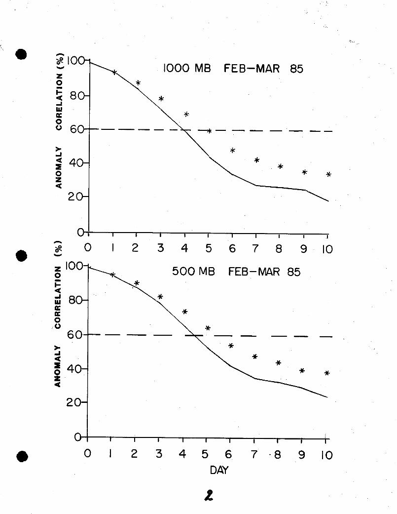
In Figures 2a and 2b the anomaly correlation obtained in the two month

period, February-March 1985, for the new MRF model is shown in comparison with

the score for the operational model at both 1000 and 500 mbs. The score was

calculated for the northern hemisphere, north of 20°N latitude, using the opera-

tional analysis to define the observed anomally.

The forecast improvement is evident after two days. Both models show

skill well above climatology throughout 10 days; the 60% level of correlation

is surpassed by the MRF model through five days, about one day more than the

operational model.

3.2 Synoptic

An interesting case, run during January 1985, contrasts the treatment

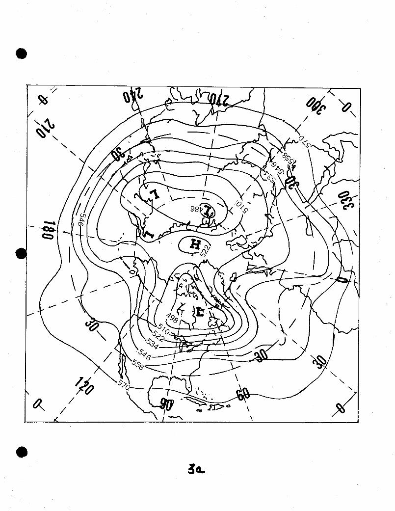
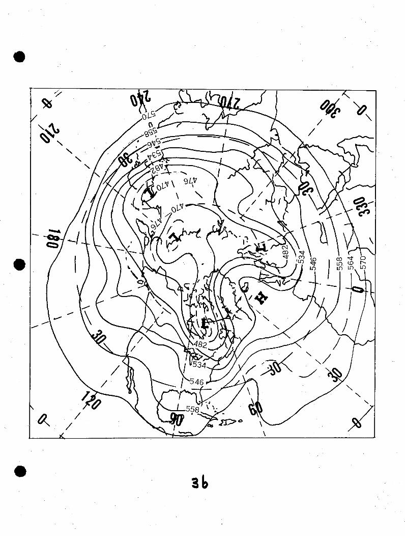
of a North Atlantic block by the MRF and operational models. Figure 3 shows

the 500 mb height field observed on January 1 and January 6, 1985. During

this 5 day period the split flow over the Atlantic is enhanced by the retro-

gression to northwestern Europe of the low initially over northern Russia.

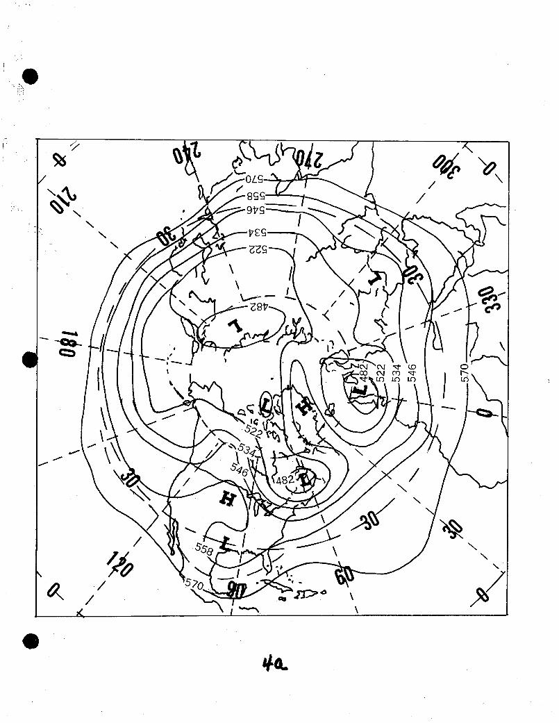
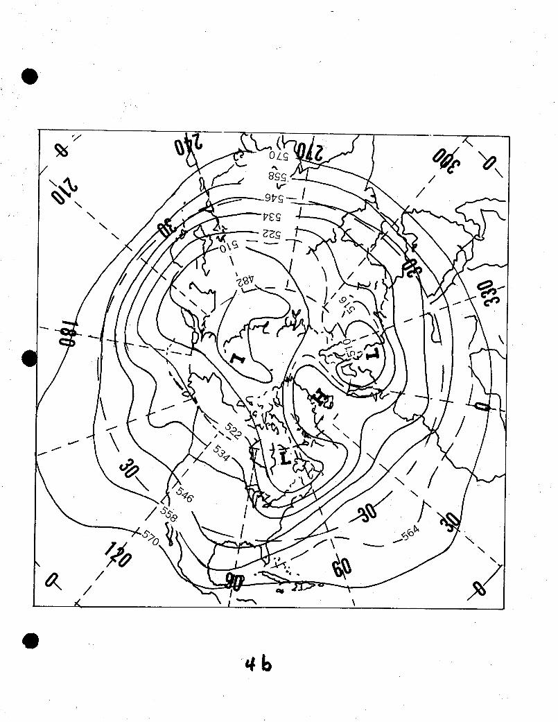
Figure 4 shows that the operational model predicted too much retrogression of

the block whereas the new MRF model provided a significantly more accurate

prediction.

8

3.3 Systematic Errors

The new MRF model parameterizes many physical processes that in nature

often tend to nearly cancel each other. In its present stage of development,

the model's physical parameterizations do not reflect the near-balances

sufficiently well and consequently systematic errors occur.

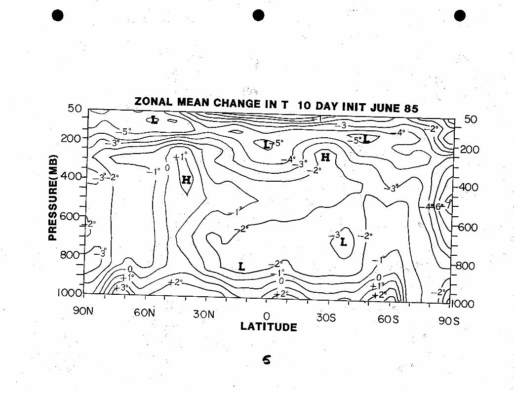
In Figure 5, the average error in zonal mean temperature in the 10-day

forecasts for June 1985 is shown. This serves to illustrate a typical

systematic error. We observe strong erroneous cooling near 150 mb at all

latitudes and, in the tropics, near 850 mb. Warming near 1000 mb is noted

between 80N and 60S. The near-surface warm bias is fully established within

the first twelve hours of the forecast; the cold bias grows gradually.

The cooling prevalent away from the surface implies that in the MRF model

radiative cooling is not compensated adequately by moist convection and sensible

heat transport. The cold bias at 850 mb between 30°N and 30°S occurs at the

level of radiative cooling atop shallow clouds and may be linked to the current

use of climatological zonally-averaged cloudiness everywhere in the MRF model.

The cooling near the tropical tropopause may largely reflect the absence of

humidity and latent heat release above 300 mb in the current MRF.

4. Summary

We have provided in this note an overview of the new NMC medium range

forecast model and its performance. Work directed toward effecting further

enhancements in the formulation of the parameterizations of physical processes

is continuing, so that a detailed description of the model is not at present

appropriate. We may note further that a development effort is now being made

to incorporate this new prediction model into the global data assimilation

system used at NMC.

9

5. Acknowledgements

J. G. Sela led the development of the-new model. The support provided to

the development of the MRF model by K. Puri, K. Miyakoda, W. Stern, S. Fels,

M. D. Schwarzkopf, J. Sirutis is gratefully acknowledged. Important contribu-

tions to the developmental testing of the new ROdil were made by many NMC

staff members, most notably, K. Campana, W. Facey, A. J. Desmarais, P. Caplan,

M. S. Tracton, M. J. Rozwodoski, F. Hughes'-and W. Collins. Special thanks

are due to F. Mesinger who provided excellent counsel on the state of the

science of medium range forecasting. Finally, we acknowledge the managerial

support and direction of W. D. Bonner, and J. A. Brown, who set high goals but

also the resources to achieve them.

0XO :0S

10

CAPTIONS FOR FIGURES

Example of change in orogrpahic field (a) mean mountains (b) silhouette

mountains.

Anomal correlation score for comparsion of older global model (solid

line) and new MRF model (asterisks) based on forecasts during February

and March 1985. (a) for 1000 mb; and (b) for 500 mb. Abscissa

shows length of forecast in days.

Analyses of observed 500-mb height for 0000 GMT 1 January 1985 (a),

6 January 1985 (b).

Forecast of 500-mb height valid for 0000 GMT 6 January 1985. (a)

older operational model; (b) new MRF model.

The monthly mean error in zonal mean temperature in 10-day, forecasts

for June 1985. Contour interval 1°C.

Figure 1.

Figure 2.

Figure 3.

Figure 4.

Figure 5.

0

OLD MEAN MTS

SILHOUETTE MTS

1

a

b

i~~ORI00--* - 1000 MB FEB-MAR 85

080-

-IC

0o 0-*

-400z

2o-

a 0 1 2 3 4 5 6 7 8 9 0z 100- 500 MB FEB-MAR 85

8-I

060 o X ~~~~~~*60- +

0 40-z

2O-

0 , i , i , i I

* 0 1 2 3 4 5 6 7 8 9 10DAY

I

30s

36

*M

-#6

0,

0

- cl

5ZONAL MEAN CHANGE IN T 10 DAY INIT JUNE 855 0 1 --

A:

=_.in

Co

ECw0.

90N 60N 30N 0 30S 60 SLATITUDE

5

90S