u t Journal of Biometrics & Biostatistics Abu Shahin et al ... · a problem of multicollinearity in the model. The biological characteristics of the human growth process were extracted

Volume 4 • Issue 2 • 1000162J Biomet BiostatISSN:2155-6180 JBMBS, an open access journal

Open Access

Abu Shahin et al., J Biomet Biostat 2013, 4:2 DOI: 10.4172/2155-6180.1000162

Open Access

Research Article

Keywords: Higher dimensional growth model; Human biologicalcharacteristics; Logistic model; Principal component regression; Bayesian approach; Velocity; Acceleration; Gradient vector; Hessian matrix

Introduction Growth modeling is very important in recent time for the purpose

of the study of growth pattern and biological characteristics. Growth in stature in any living organism depends on their: age, body weight, chest circumference, sitting height, genetic factors, maternal illnesses during pregnancy, socio-economic disadvantages during and after pregnancy, social/emotional problems during childhood, poor nutrition and environmental or emotional deprivation and so on. Most of the growth models such as Gompertz and the logistic growth model [1,2], Jenss model [3], Count model [4,5] , Double logistic model [6], PB models [7,8], ICP model [9], Reed models [10], SSC model [8,11], JPPS model [12], JPA-1 and JPA-2 model [13], Modified ICP model [14], BTT model [15] have considered stature or weight as a function of age. Comparative study among different fitted growth models was done by many authors [8,16,17]. The JPA-2 [13] model fits better than all other asymptotic models till 1991. While, BTT [18] model is found to be better than JPA-2 model. Like age, it is important to incorporate other possible predictors in the model as they have significant influence on stature, however, the influence of age on stature is higher than others predictors.

Thus, for the better explanation of the final stature, higher dimensional growth model should be applicable. Rahman et al. [19] showed that the BTT model fits better for those who have early, middle and adolescent growth spurts.

Thus, the purpose of the present study is to develop a higher dimensional growth model through the extension of BTT model.

History of the BTT ModelRobertson [20] proposed that the human growth of organism in

general occurs in a number of additive, more-or-less independent phases during the course of development. Generally, the timing and intensity of each phase is assumed genetically programmed in the individual, but they may vary in expression according to environmental conditions. According to Robertson, the sum of the three logistic components can be describing human growth in stature but he cannot test the model because of no suitable data. Bock and Thissen (1976) [21], first applied the concept to individual growth using the case from the Berkeley and Fels growth studies. Their analysis showed that the goodness of fit of the triphasic logistic model was good over the range

from one year to maturity. In the Bock-Thissen model, the phases represent early-childhood, middle-childhood, and adolescent growth. A further enhancement of the Bock-Thissen model was suggested by du Toit [22]. du Toit [22] suggested the additional of the “shape” constants of the positive exponentials to the denominators of the logistic functions to control the model in the region of change-over from early to middle childhood, and to provide some asymmetry of the adolescent component. We found values for these constants that tend to improve the fit of the model, by repeated trials with the Berkeley and Fels data. We refer to this triphasic generalized logistic model as the BTT model.

Mathematical Explanation of the BTT ModelBock-Thissen-du Toit (BTT) model can be defined as sum of the

three generalized logistic terms. The form of the logistic term is:

( )1dbt c

a

e +− + where, t is the time (age) variable; a, b, c and d are the amount of growth, slope, intercept and fixed shape constant contributed by the term, respectively. The quantity z=(bt+c) in the exponential function is the “logit”.

Bock et al. [15] described a model known as the triphasic generalized logistic model by summing up three phases of growth; early, middle and adolescent. This triphasic generalized logistic model can be written as follows:

( ) ( ) ( )1 2 31 1 2 2 3 3

31 2

1 1 1d d db t c b t c b t c

aa aye e e+ + +− − −

= + + + + +

where, the set of parameters (a1,b1,c1), (a2,b2,c2) and (a3,b3,c3) refer to the parameters of early, middle and adolescent phases of growth, respectively.

*Corresponding author: Md. Ayub Ali, Department of Statistics, University of Rajshahi, Rajshahi-6205, Bangladesh, E-mail: [email protected]

Received January 28, 2013; Accepted March 02, 2013; Published March 08, 2013

Citation: Abu Shahin Md, Ayub Ali Md, Shawkat Ali ABM (2013) An Extension of Generalized Triphasic Logistic Human Growth Model. J Biomet Biostat 4: 162. doi:10.4172/2155-6180.1000162

Copyright: © 2013 Abu Shahin Md, et al. This is an open-access article distributed under the terms of the Creative Commons Attribution License, which permits unrestricted use, distribution, and reproduction in any medium, provided the original author and source are credited.

An Extension of Generalized Triphasic Logistic Human Growth ModelMd. Abu Shahin1, Md. Ayub Ali1* and A. B. M. Shawkat Ali2

1Department of Statistics, University of Rajshahi, Rajshahi-6205, Bangladesh2School of ICT, Central Queensland University, QLD 4702, Australia

AbstractThe purpose of the present study was to establish an extension of generalized tri-phasic logistic human growth

model. This model was applied through the higher dimensional growth process. Bayesian method of estimation was applied to estimate the parameters of the model. Principal component regression method was applied when there was a problem of multicollinearity in the model. The biological characteristics of the human growth process were extracted from the velocity and acceleration curve using gradient vector and Hessian matrix.

Journal of Biometrics & Biostatistics Jour

nal o

f Biometrics & Biostatistics

ISSN: 2155-6180


J Biomet BiostatISSN:2155-6180 JBMBS, an open access journal

Page 2 of 7

Volume 4 • Issue 2 • 1000162

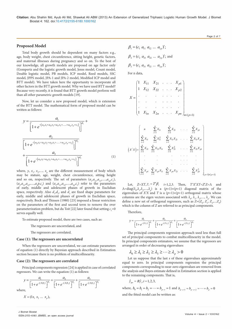
Proposed ModelTotal body growth should be dependent on many factors e.g.,

age, body weight, chest circumference, sitting height, genetic factors, and maternal illnesses during pregnancy and so on. To the best of our knowledge, all growth models are proposed on age factor only (Gompertz and the logistic growth model, Jenss model, Count model, Double logistic model, PB models, ICP model, Reed models, SSC model, JPPS model, JPA-1 and JPA-2 model, Modified ICP model and BTT model). We have taken here the opportunity to incorporate all other factors in the BTT growth model. Why we have used BTT model? Because very recently, it is found that BTT growth model perform well than all other parametric growth models [19].

Now, let us consider a new proposed model, which is extension of the BTT model. The mathematical form of proposed model can be written as follows:

( )

( )

111 1 12 2 13 3 1 1

221 1 22 2 23 3 2 2

1

......

2

......

1

1

p p

p p

da x a x a x a x c

da x a x a x a x c

aye

a

e

− + + + + +

− + + + + +

= + +

+

( ) 331 1 32 2 33 3 3 3

3

......1 p pd

a x a x a x a x c

a

e− + + + + ++ +

(1)

where, y, x1, x2,...., xp are the different measurement of body which may be stature, age, weight, chest circumference, sitting height and so on, respectively. The set of parameters (a1,a11,a12,.....,a1p,c1), (a2,a21,a22,.....,a2p,c2) and (a3,a31,a32,.....,a3p,c3) refer to the parameters of early, middle and adolescent phases of growth in Euclidian space, respectively. Also d1,d2, and d3 are fixed shape parameters for early, middle and adolescent phases of growth in Euclidian space, respectively. Bock and Thissen (1980) [23] imposed a linear restriction on the parameters of the first and second term to remove the over parameterization problem, but du Toit [22] later found that setting c1=0 serves equally well.

To estimate proposed model, there are two cases, such as:

The regressors are uncorrelated, and

The regressors are correlated.

Case (1): The regressors are uncorrelated

When the regressors are uncorrelated, we can estimate parameters of equation (1) directly by Bayesian approach described in Estimation section because there is no problem of multicollinearity.

Case (2): The regressors are correlated

Principal components regression [24] is applied in case of correlated regressors. We can write the equation (1) as follows:

( ) ( ) ( )1 2 31 2 3

31 2

1 1 1d d dX X X

aa aye e eβ β β− − −

= + + + + +

where,

1 2(1 ... ),pX x x x=

For n data,

11 21 1

12 22 2

1 2 ( 1)

1 . . .

1 . . .

. . . . . . .

. . . . . . .

. . . . . . .1 . . .

p

p

n n pn n p

X X X

X X X

X

X X X× +

=

( )

1 21 1 1

21 1 1 2 1

1 1 1 1

2/ 2 2 1 2 2

1 1 1 1

21 2

1 1 1 1

. . .

. . .

. . .

. . . . . . .

. . . . . . .

. . . . . . .

. . .

n n n

i i pii i i

n n n n

i i i i i pii i i in n n n

i i i i i pii i i i

n n n n

pi pi i pi i pii i i i

n X X X

X X X X X X

X X X X X XX X

X X X X X X

= = =

= = = =

= = = =

= = = =

=

∑ ∑ ∑

∑ ∑ ∑ ∑

∑ ∑ ∑ ∑

∑ ∑ ∑ ∑( ) ( )1 1p p+ × +

Therefore,

( ) ( ) ( )1 2 31 2 3

31 2

1 1 1d d dZ Z Z

aa aye e eγ γ γ− − −

= + + + + +

The principal components regression approach used less than full set of principal components to combat multicollinearity in the model. In principal components estimators, we assume that the regressors are arranged in order of decreasing eigenvalues:

0 1 2 3 0pλ λ λ λ λ≥ ≥ ≥ ≥ ≥ >

Let us suppose that the last s of these eigenvalues approximately equal to zero. In principal components regression the principal components corresponding to near-zero eigenvalues are removed from the analysis and Bayes estimate defined in Estimation section is applied to the remaining components. That is,

ˆ ˆ , 1, 2,3,ipc iB iγ γ= =

where, 0 1 2 1p sb b b b −= = = = = and 1 2 0p s p s pb b b− + − += = = =

and the fitted model can be written as:

1 1 11 12 1( ... ) ;pc a a aβ ′=

2 2 21 22 2( ... ) ;pc a a aβ ′= and

3 3 31 32 3( ... ) ;pc a a aβ ′=

Let, Z=XT, i iTγ β′= i=1,2,3. Then, T′X′XT=Z′Z=Λ and Λ=diag(λ0,λ1,λ2,....,λp) is a (p+1)×(p+1) diagonal matrix of the eigenvalues of X’X and T is a (p+1)×(p+1) orthogonal matrix whose columns are the eigen vectors associated with λ0, λ1, λ2,...., λp. We can define a new set of orthogonal regressors, such as Z=(Z0, Z1, Z2,....ZP) which is the column of Z are referred to as principal components.



Page 3 of 7

Volume 4 • Issue 2 • 1000162

( ) ( ) ( )1 2 3

1 2 3

31 2

ˆ ˆ ˆˆ

1 1 1d d dZ Z Z


= + + + + +

Replacing Z by the linear combination of X, we get

( ) ( ) ( )1 2 3

1 2 3

31 2

ˆ ˆ ˆˆ

1 1 1d d dXT XT XT


= + + + + +

( ) ( ) ( )1 2 31 2 3

31 2

ˆ ˆ ˆˆ

1 1 1pc pc pcd d d

X X X

aa aye e eβ β β− − −

= + + + + +

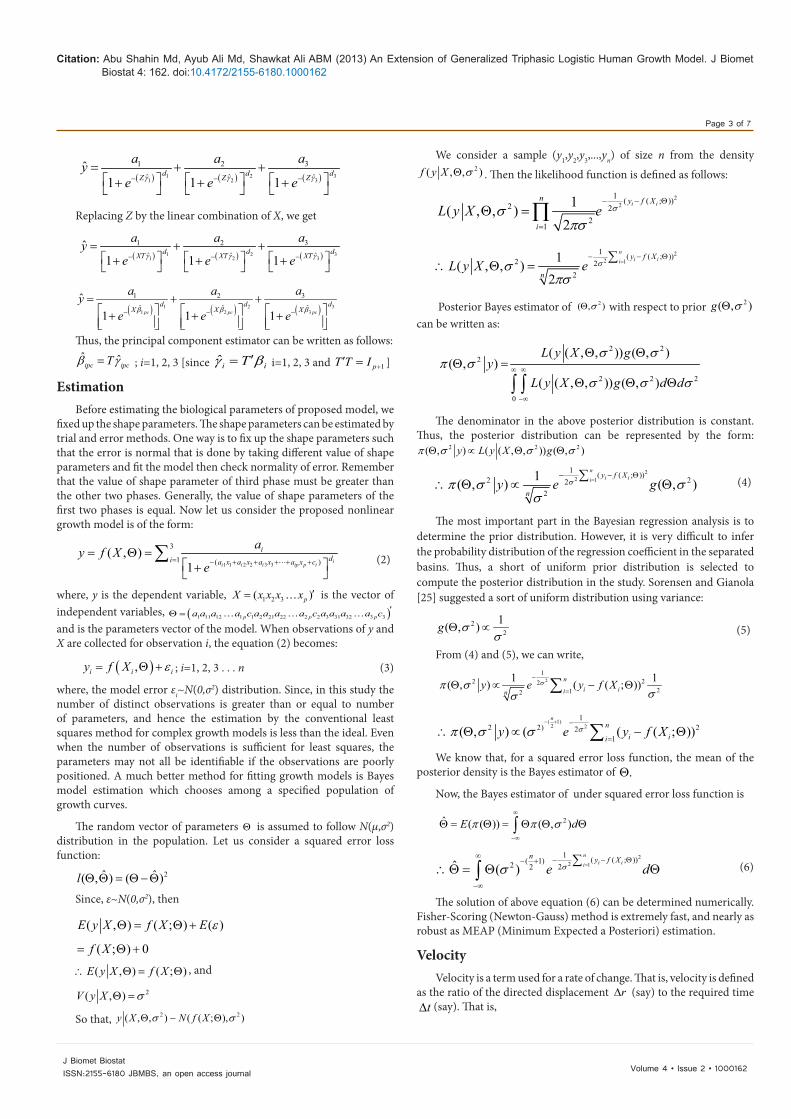
Thus, the principal component estimator can be written as follows:

EstimationBefore estimating the biological parameters of proposed model, we

fixed up the shape parameters. The shape parameters can be estimated by trial and error methods. One way is to fix up the shape parameters such that the error is normal that is done by taking different value of shape parameters and fit the model then check normality of error. Remember that the value of shape parameter of third phase must be greater than the other two phases. Generally, the value of shape parameters of the first two phases is equal. Now let us consider the proposed nonlinear growth model is of the form:

1 1 2 2 3 3

3

1 ( )( , )

1ii i i ip p i

idi a x a x a x a x c

ay f Xe

= − + + + + += Θ =

+ ∑

(2)

( ),i i iy f X ε= Θ + ; i=1, 2, 3 . . . n (3)

where, the model error εi~N(0,σ2) distribution. Since, in this study the number of distinct observations is greater than or equal to number of parameters, and hence the estimation by the conventional least squares method for complex growth models is less than the ideal. Even when the number of observations is sufficient for least squares, the parameters may not all be identifiable if the observations are poorly positioned. A much better method for fitting growth models is Bayes model estimation which chooses among a specified population of growth curves.

The random vector of parameters Θ is assumed to follow N(μ,σ2) distribution in the population. Let us consider a squared error loss function:

2ˆ ˆ( , ) ( )l Θ Θ = Θ−Θ

Since, ε~N(0,σ2), then

( , ) ( ; ) ( )E y X f X E εΘ = Θ +

( ; ) 0f X= Θ +

( , ) ( ; )E y X f X∴ Θ = Θ , and

2( , )V y X σΘ =

So that, 2 2( , , ) ( ( ; ), )y X N f Xσ σΘ Θ

We consider a sample (y1,y2,y3,...,yn) of size n from the density 2( , , )f y X σΘ . Then the likelihood function is defined as follows:

22

1 ( ( ; ))2 22

1

1( , , )2

i in y f X

i

L y X e σσπσ

− − Θ

=

Θ =∏

22 1

1 ( ( ; ))2 22

1( , , )2

ni ii

y f X

nL y X e σσ

πσ=

− − Θ∑∴ Θ =

Posterior Bayes estimator of 2( , )σΘ with respect to prior 2( , )g σΘ can be written as:

2 22

2 2 2

0

( ( , , )) ( , )( , )

( ( , , )) ( , )

L y X gy

L y X g d d

σ σπ σ

σ σ σ∞ ∞

−∞

Θ ΘΘ =

Θ Θ Θ∫ ∫

The denominator in the above posterior distribution is constant. Thus, the posterior distribution can be represented by the form:

2 2 2( , ) ( ( , , )) ( , )y L y X gπ σ σ σΘ ∝ Θ Θ

22 1

1 ( ( ; ))2 222

1( , ) ( , )n

i iiy f X

ny e gσπ σ σ

σ=

− − Θ∑∴ Θ ∝ Θ (4)

The most important part in the Bayesian regression analysis is to determine the prior distribution. However, it is very difficult to infer the probability distribution of the regression coefficient in the separated basins. Thus, a short of uniform prior distribution is selected to compute the posterior distribution in the study. Sorensen and Gianola [25] suggested a sort of uniform distribution using variance:

22

1( , )g σσ

Θ ∝ (5)

From (4) and (5), we can write,

21

2 22212

1 1( , ) ( ( ; ))ni iin

y e y f Xσπ σσσ

−

=Θ ∝ − Θ∑

( 1)2 2

12 2) 22

1( , ) ( ( ( ; ))

nn

i iiy e y f Xσπ σ σ

− + −

=∴ Θ ∝ − Θ∑We know that, for a squared error loss function, the mean of the

posterior density is the Bayes estimator of .Θ

Now, the Bayes estimator of under squared error loss function is

2ˆ ( ( )) ( , )E dπ π σ∞

−∞

Θ = Θ = Θ Θ Θ∫

2

2 11 ( ( ; ))( 1)2 22ˆ ( )

ni ii

n y f Xe dσσ =

∞ − − Θ− +

−∞

∑∴Θ = Θ Θ∫ (6)

The solution of above equation (6) can be determined numerically. Fisher-Scoring (Newton-Gauss) method is extremely fast, and nearly as robust as MEAP (Minimum Expected a Posteriori) estimation.

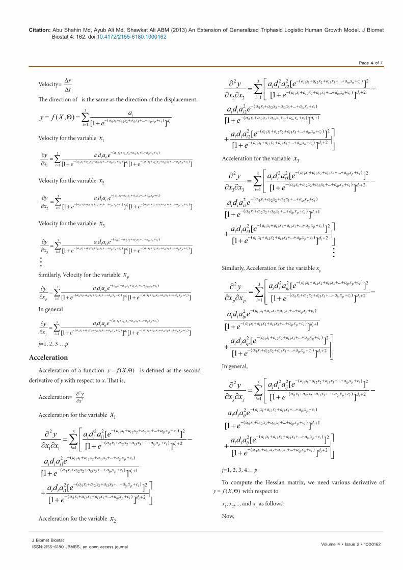
VelocityVelocity is a term used for a rate of change. That is, velocity is defined

as the ratio of the directed displacement r∆ (say) to the required time t∆ (say). That is,

ˆ ˆipc ipcTβ γ= ; i=1, 2, 3 [since i iTγ β′= i=1, 2, 3 and 1pT T I +′ = ]

where, y is the dependent variable, 1 2 3( )pX x x x x ′= is the vector of independent variables, ( )1 11 12 1 1 2 21 22 2 2 3 31 32 3 3p p pa a a a c a a a a c a a a a c ′Θ =

and is the parameters vector of the model. When observations of y and X are collected for observation i, the equation (2) becomes:



Page 4 of 7

Volume 4 • Issue 2 • 1000162

Velocity= rt

∆∆

The direction of is the same as the direction of the displacement.

1 1 2 2 3 3

3

( ... )1

( , )[1 ]i i i ip p i i

ia x a x a x a x c d

i

ay f Xe− + + + + +

=

= Θ =+

∑

Velocity for the variable 1x

1 1 2 2 3 3

1 1 2 2 3 3 1 1 2 2 3 3

( ... )31

( ... ) ( ... )11 [1 ] [1 ]

i i i ip p i

i i i ip p i i i i ip p ii

a x a x a x a x ci i i

a x a x a x a x c a x a x a x a x cdi

a d a eyx e e

− + + + + +

− + + + + + − + + + + +=

∂=

∂ + +∑


1 1 2 2 3 3

1 1 2 2 3 3 1 1 2 2 3 3

( ... )32

( ... ) ( ... )12 [1 ] [1 ]

i i i ip p i




a d a eyx e e

− + + + + +

− + + + + + − + + + + +=

∂=

∂ + +∑


1 1 2 2 3 3

1 1 2 2 3 3 1 1 2 2 3 3

( ... )33

( ... ) ( ... )13 [1 ] [1 ]

i i i ip p i




a d a eyx e e

− + + + + +

− + + + + + − + + + + +=

∂=

∂ + +∑

Similarly, Velocity for the variable px

1 1 2 2 3 3

1 1 2 2 3 3 1 1 2 2 3 3

( ... )3

( ... ) ( ... )1 [1 ] [1 ]

i i i ip p i


a x a x a x a x ci i ip

a x a x a x a x c a x a x a x a x cdip

a d a eyx e e

− + + + + +

− + + + + + − + + + + +=

∂=

∂ + +∑

In general

1 1 2 2 3 3

1 1 2 2 3 3 1 1 2 2 3 3

( ... )3

( ... ) ( ... )1 [1 ] [1 ]

i i i ip p i


a x a x a x a x ci i ij

a x a x a x a x c a x a x a x a x cdij

a d a eyx e e

− + + + + +

− + + + + + − + + + + +=

∂=

∂ + +∑

j=1, 2, 3 …p

Acceleration

Acceleration of a function ( , )y f X= Θ is defined as the second

derivative of y with respect to x. That is,

Acceleration= 2

2

yx∂∂

Acceleration for the variable 1x

1 1 2 2 3 3

1 1 2 2 3 3

1 1 2 2 3 3

1 1 2 2 3 3

( ... )2 2 22 31( ... ) 2

11 1

( ... )21( ... ) 1

21

[ ][1 ]

[1 ]

i i i ip p i

i i i ip p i i

i i i ip p i

i i i ip p i i


a x a x a x a x c di


a x a x a x a x c d

i i i

a d a eyx x e

a d a ee

a d a

− + + + + +

− + + + + + +=

− + + + + +

− + + + + + +

∂= −∂ ∂ +

+

+

∑

1 1 2 2 3 3

1 1 2 2 3 3

( ... ) 2

( ... ) 2

[ ][1 ]

i i i ip p i

i i i ip p i i

a x a x a x a x c

a x a x a x a x c d

ee

− + + + + +

− + + + + + +

+


1 1 2 2 3 3

1 1 2 2 3 3

1 1 2 2 3 3

1 1 2 2 3 3

( ... )2 2 22 32( ... ) 2

12 2

( ... )22( ... ) 1

22

[ ][1 ]

[1 ]

i i i in n i

i i i in n i i

i i i in n i

i i i in n i i




a x a x a x a x c d

i i i

a d a eyx x e

a d a ee

a d a

− + + + + +

− + + + + + +=

− + + + + +

− + + + + + +

∂= −∂ ∂ +

+

+

∑

1 1 2 2 3 3

1 1 2 2 3 3

( ... ) 2

( ... ) 2

[ ][1 ]

i i i in n i

i i i in n i i

a x a x a x a x c

a x a x a x a x c d

ee

− + + + + +

− + + + + + +

+


1 1 2 2 3 3

1 1 2 2 3 3

1 1 2 2 3 3

1 1 2 2 3 3

( ... )2 2 22 33( ... ) 2

13 3

( ... )23( ... ) 1

23

[ ][1 ]

[1 ]

i i i ip p i

i i i ip p i i

i i i ip p i

i i i ip p i i




a x a x a x a x c d

i i i

a d a eyx x e

a d a ee

a d a

− + + + + +

− + + + + + +=

− + + + + +

− + + + + + +

∂= −∂ ∂ +

+

+

∑

1 1 2 2 3 3

1 1 2 2 3 3

( ... ) 2

( ... ) 2

[ ][1 ]

i i i ip p i

i i i ip p i i

a x a x a x a x c

a x a x a x a x c d

ee

− + + + + +

− + + + + + +

+

Similarly, Acceleration for the variable xp

1 1 2 2 3 3

1 1 2 2 3 3

1 1 2 2 3 3

1 1 2 2 3 3

( ... )2 2 22 3

( ... ) 21

( ... )2

( ... ) 1

[ ][1 ]

[1 ]

i i i ip p i

i i i ip p i i

i i i ip p i

i i i ip p i i


a x a x a x a x c dip p


a x a x a x a x c d

i i ip

a d a eyx x e

a d a ee

a d a

− + + + + +

− + + + + + +=

− + + + + +

− + + + + + +

∂= −

∂ ∂ +

+

+

∑

1 1 2 2 3 3

1 1 2 2 3 3

( ... )2 2

( ... ) 2

[ ][1 ]

i i i ip p i

i i i ip p i i

a x a x a x a x c

a x a x a x a x c d

ee

− + + + + +

− + + + + + +

+ In general,

1 1 2 2 3 3

1 1 2 2 3 3

1 1 2 2 3 3

1 1 2 2 3 3

( ... )2 2 22 3

( ... ) 21

( ... )2

( ... ) 1

[ ][1 ]

[1 ]

i i i ip p i

i i i ip p i i

i i i ip p i

i i i ip p i i


a x a x a x a x c dij j


a x a x a x a x c d

i i ij

a d a eyx x e

a d a ee

a d a

− + + + + +

− + + + + + +=

− + + + + +

− + + + + + +

∂= −

∂ ∂ +

+

+

∑

1 1 2 2 3 3

1 1 2 2 3 3

( ... )2 2

( ... ) 2

[ ][1 ]

i i i ip p i

i i i ip p i i

a x a x a x a x c

a x a x a x a x c d

ee

− + + + + +

− + + + + + +

+

j=1, 2, 3, 4… p

To compute the Hessian matrix, we need various derivative of ( , )y f X= Θ with respect to

x1, x2,..., and xp as follows:

Now,



Page 5 of 7

Volume 4 • Issue 2 • 1000162

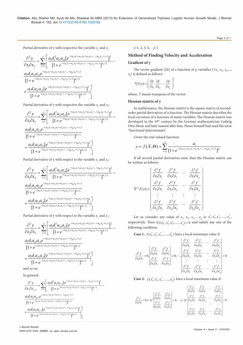
Partial derivative of y with respective the variable x1 and x2

1 1 2 2 3 3

1 1 2 2 3 3

1 1 2 2 3 3

1 1 2 2 3 3

( ... )2 22 31 2

( ... ) 211 2

( ... )1 2

( ... ) 1

[ ][1 ]

[1 ]

i i i ip p i

i i i ip p i i

i i i ip p i

i i i ip p i i

a x a x a x a x ci i i i



a x a x a x a x c d

i i

a d a a eyx x e

a d a a ee

a d

− + + + + +

− + + + + + +=

− + + + + +

− + + + + + +

∂= −∂ ∂ +

+

+

∑

1 1 2 2 3 3

1 1 2 2 3 3

( ... ) 21 2

( ... ) 2

[ ][1 ]

i i i ip p i

i i i ip p i i

a x a x a x a x ci i

a x a x a x a x c d

a a ee

− + + + + +

− + + + + + +

+

Partial derivative of y with respective the variable x1 and x3:

1 1 2 2 3 3

1 1 2 2 3 3

1 1 2 2 3 3

1 1 2 2 3 3

( ... )2 22 31 3

( ... ) 211 3

( ... )1 3

( ... ) 1

[ ][1 ]

[1 ]

i i i ip p i

i i i ip p i i

i i i ip p i

i i i ip p i i




a x a x a x a x c d

i i

a d a a eyx x e

a d a a ee

a d

− + + + + +

− + + + + + +=

− + + + + +

− + + + + + +

∂= −∂ ∂ +

+

+

∑

1 1 2 2 3 3

1 1 2 2 3 3

( ... ) 21 3

( ... ) 2

[ ][1 ]

i i i ip p i

i i i ip p i i


a x a x a x a x c d

a a ee

− + + + + +

− + + + + + +

+

1 1 2 2 3 3

1 1 2 2 3 3

1 1 2 2 3 3

1 1 2 2 3 3

( ... )2 22 31 4

( ... ) 211 4

( ... )1 4

( ... ) 1

[ ][1 ]

[1 ]

i i i ip p i

i i i ip p i i

i i i ip p i

i i i ip p i i




a x a x a x a x c d

i i

a d a a eyx x e

a d a a ee

a d

− + + + + +

− + + + + + +=

− + + + + +

− + + + + + +

∂= −∂ ∂ +

+

+

∑

1 1 2 2 3 3

1 1 2 2 3 3

( ... ) 21 4

( ... ) 2

[ ][1 ]

i i i ip p i

i i i ip p i i


a x a x a x a x c d

a a ee

− + + + + +

− + + + + + +

+

1 1 2 2 3 3

1 1 2 2 3 3

1 1 2 2 3 3

1 1 2 2 3 3

( ... )2 22 32 3

( ... ) 212 3

( ... )2 3

( ... ) 1

[ ][1 ]

[1 ]

i i i ip p i

i i i ip p i i

i i i ip p i

i i i ip p i i




a x a x a x a x c d

i i

a d a a eyx x e

a d a a ee

a d

− + + + + +

− + + + + + +=

− + + + + +

− + + + + + +

∂= −∂ ∂ +

+

+

∑

1 1 2 2 3 3

1 1 2 2 3 3

( ... ) 22 3

( ... ) 2

[ ][1 ]

i i i ip p i

i i i ip p i i


a x a x a x a x c d

a a ee

− + + + + +

− + + + + + +

+ and so on.

In general:

1 1 2 2 3 3

1 1 2 2 3 3

1 1 2 2 3 3

1 1 2 2 3 3

( ... )2 22 31

( ... ) 211

( ... )1

( ... )

[ ][1 ]

[1 ]

i i i ip p i

i i i ip p i i

i i i ip p i

i i i ip p i i

a x a x a x a x ci i ij ij

a x a x a x a x c dij j


a x a x a x a x c d

a d a a eyx x e

a d a a ee

− + + + + ++

− + + + + + +=+

− + + + + ++

− + + + + +

∂= −

∂ ∂ +

+

∑

1 1 2 2 3 3

1 1 2 2 3 3

1

( ... ) 21

( ... ) 2

[ ][1 ]

i i i ip p i

i i i ip p i i


a x a x a x a x c d

a d a a ee

+

− + + + + ++

− + + + + + +

+

+

j=1, 2, 3, 4… p-1

Method of Finding Velocity and AccelerationGradient of y

The vector gradient [26] of a function of p variables f (x1, x2, x3,..., xp) is defined as follows:

1 2

( )T

p

f f ff xx x x

∂ ∂ ∂∇ = ∂ ∂ ∂

where, T means transpose of the vector.

Hessian matrix of y

In mathematics, the Hessian matrix is the square matrix of second-order partial derivatives of a function. The Hessian matrix describes the local curvature of a function of many variables. The Hessian matrix was developed in the 19th century by the German mathematician Ludwig Otto Hesse and later named after him. Hesse himself had used the term “functional determinants”.

Given the real-valued function:

1 1 2 2 3 3

3

( ... )1

( , )[1 ]i i i ip p i i

ia x a x a x a x c d

i

ay f Xe− + + + + +

=

= Θ =+

∑If all second partial derivatives exist, then the Hessian matrix can

be written as follows:

2 2 2

1 1 1 2 1

2 2 2

22 1 2 2 2

2 2 2

1 2

( )

p

p

p p p p

f f fx x x x x x

f f fx x x x x xf x

f f fx x x x x x

∂ ∂ ∂ ∂ ∂ ∂ ∂ ∂ ∂ ∂ ∂ ∂ ∂ ∂ ∂ ∂ ∂ ∂∇ =

∂ ∂ ∂ ∂ ∂ ∂ ∂ ∂ ∂

Let us consider any value of x1, x2, x3, ...xp is * * * *

1 2 3, , ,......, px x x x , respectively. Then * * * *

1 2 3( , , ,......, ) 0pf x x x x∇ = and satisfy any one of the following condition:

Case 1: * * * *1 2 3( , , ,......, )pf x x x x have a local minimum value if:

2 2 2

1 1 1 2 12 22 2 2

21 1 1 2

2 1 2 2 22 21 1

2 1 2 2 2 2 2

1 2

0, 0, , 0

p

p

p p p p

f f fx x x x x x

f ff f f

x x x xf x x x x x xx x f f

x x x xf f f

x x x x x x

∂ ∂ ∂∂ ∂ ∂ ∂ ∂ ∂

∂ ∂∂ ∂ ∂

∂ ∂ ∂ ∂∂ ∂ ∂ ∂ ∂ ∂ ∂> > >∂ ∂ ∂ ∂

∂ ∂ ∂ ∂∂ ∂ ∂∂ ∂ ∂ ∂ ∂ ∂

Case 2: * * * *1 2 3( , , ,......, )pf x x x x have a local maximum value if:

2 2 2

1 1 1 2 12 22 2 2

21 1 1 22

2 1 2 2 22 21 1

2 1 2 2 2 2 2

1 2

0, ( 1) 0, , ( 1) 0

p

pp

p p p p

f f fx x x x x x

f ff f f

x x x xy x x x x x xx x f f

x x x xf f f

x x x x x x

∂ ∂ ∂∂ ∂ ∂ ∂ ∂ ∂

∂ ∂∂ ∂ ∂

∂ ∂ ∂ ∂∂ ∂ ∂ ∂ ∂ ∂ ∂< − > − >∂ ∂ ∂ ∂

∂ ∂ ∂ ∂∂ ∂ ∂∂ ∂ ∂ ∂ ∂ ∂

Partial derivative of y with respect to the variable x1 and x2:

Partial derivative of y with respect to the variable x2 and x3:



Page 6 of 7

Volume 4 • Issue 2 • 1000162

Case 3: There is no local maxima or minima if * * * *1 2 3( , , ,......, )pf x x x x

Numerical ExampleConsider the longitudinal data of Japanese girl from 1 year to 18 year.

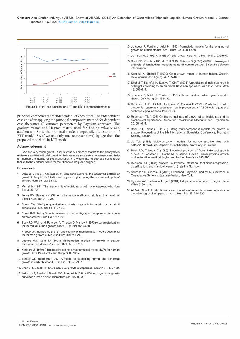
The data contains the variables age, stature and chest circumference. We used the STATISTICA software to estimate the parameters and the MatLab software help us to find the velocity and acceleration with respect to different variables. Let us consider the case-1, when the regressors are uncorrelated. We have used the study variables such as age and stature for BTT, and age, stature and chest circumference for proposed models. The Bayesian approach with squared error loss function used for estimated parameters and Quasi-Newton method is used for iterations process. The estimated parameters and final loss (sum of squared error) for the BTT and proposed models are presented in table 1. We have used various values of shape constants (d1, d2 and d3) for comparative study of BTT and proposed models. From table 1, we see that for the same value of shape constants, BTT and proposed models have different values of final loss. The model gives smallest values of final loss considered as best model. From table 1, the proposed model gives smallest values of final loss, compared with BTT model for same shape constants. Therefore, the proposed model is more

accurate than BTT model because it explains stature efficiently with small error compared with BTT model. The plot of final loss function corresponding to BTT and EBTT (Proposed) models are shown in figure 1. From figure 1, it is clear that within the acceptable region of shape constants, the loss function for EBTT model is always smaller than BTT model.

The default values of the shape constants given in the Auxal software [15] were also applicable for Japanese population [27]. Thus the values of d1, 2 and d3 are considered as 0.75, 0.75 and 1.20, respectively. Therefore, the velocity and acceleration for the proposed model with shape constants of d1=0.75, d2=0.75 and d3=1.20 are presented in table 2. The estimated parameters of the proposed model is presented last row of table 1.

ConclusionThe proposed extension of BTT model is very important because

the stature of human depends on several factors. In BTT model, we only know the impact of age on stature but our proposed model study knows the impact of several factors. There are more than one variable in the regressors, so the multicollinearity problem may arise. In this case, we can apply principal component regression method for regressor’s variables and find a few components. The advantage of PCA is that the

ParameterModel 1d 2d

3d1a 11a 12a

1c 2a 21a 22a 2c3a 31a 32a 3c Final loss

BTT 0.75 0.75 0.75 27.60 0.81 -9.10 140.63 0.27 -0.55 -2.62 2.23 -18.77 5.01EBTT 0.75 0.75 0.75 -10.84 52.05 1.06 -0.16 -0.36 93.59 1.04 -0.18 8.24 18.28 1.45 0.08 1.16BTT 0.50 0.75 0.75 -32.24 -0.94 9.65 118.58 0.34 -1.13 78.94 -0.04 0.72 4.26EBTT 0.50 0.75 0.75 54.68 1.07 -0.15 -1.97 98.54 0.61 -0.04 1.91 10.63 2.56 -0.21 -0.85 1.29BTT 0.60 0.80 0.80 40.42 -3.03 126.19 90.58 0.40 -1.23 33.20 0.77 -8.76 4.62EBTT 0.60 0.80 0.80 45.49 0.69 0.32 -31.18 23.04 1.80 -1.62 91.65 119.18 0.33 -0.01 -0.31 2.15BTT 0.70 0.80 0.90 -32.20 -0.82 8.72 106.43 0.35 -1.12 82.56 -0.03 1.21 4.37EBTT 0.70 0.80 0.90 36.07 0.96 -0.05 -7.63 83.08 0.48 -0.02 -0.32 45.42 1.69 -0.92 48.70 2.88BTT 0.75 0.75 1.20 90.05 0.41 -1.32 34.20 0.77 -8.86 39.90 1.84 62.41 4.63EBTT 0.75 0.75 1.20 74.12 1.23 -0.47 22.04 52.70 0.34 0.12 -7.73 37.35 0.91 -0.07 -4.54 3.29

Note: BTT and EBTT means Bock-Thissen-du Toit and Extension of Bock-Thissen-du Toit model, respectively. Table 1: Estimated parameters and final loss for BTT and proposed models.

Stature Predicted Error Fx1 Fx2 Fx1x1 Fx2x2 Fx1x2 Det(H) Comment75 75.48 -0.480 12.24 -2.78 -8.068 -1.189 3.418 -2.09 Saddle84 83.01 0.993 11.13 -1.79 -7.008 -1.036 2.996 -1.72 Saddle92 92.21 -0.207 7.989 -0.22 -4.136 -0.620 1.810 -0.72 Saddle99 99.78 -0.784 8.993 -0.42 -5.075 -0.761 1.919 0.18 L. Max108 107.69 0.310 7.693 -0.17 -4.113 -0.648 1.404 0.69 L. Max115 114.57 0.430 5.797 0.281 -1.651 -0.371 0.565 0.29 L. Max120 120.30 -0.301 5.745 0.047 -0.068 -0.289 0.298 -0.07 L. Max126 125.78 0.220 6.959 -0.26 1.674 -0.211 0.092 -0.36 Saddle131 131.39 -0.391 9.191 -0.76 1.542 -0.227 0.236 -0.405 Saddle138 137.85 0.149 10.83 -1.12 -0.913 -0.267 0.552 -0.06 Saddle145 144.74 0.255 10.46 -1.26 -4.136 -0.323 0.922 0.495 L. Max152 152.16 -0.156 7.547 -0.94 -4.858 -0.256 0.842 0.534 L. Max156 156.37 -0.366 5.421 -0.88 -4.543 -0.292 0.913 0.491 L. Max160 159.77 0.229 3.216 -0.60 -3.045 -0.220 0.667 0.225 L. Max163 162.46 0.541 1.236 -0.19 -1.187 -0.069 0.222 0.033 L. Max163 163.03 -0.025 0.875 -0.19 -0.912 -0.079 0.228 0.020 L. Max163 163.50 -0.496 0.532 -0.14 -0.578 -0.059 0.163 0.007 L. Max164 163.93 0.066 0.182 -0.04 -0.192 -0.018 0.050 0.001 L. Max

Note: Fx1, Fx2, Fx1x1, Fx2x2, Fx1x2 and Det (H) denote the velocity with respect to age and chest circumference, acceleration with respect to age and chest circumference, the partial derivative with respect to age and chest circumference and determinant of 2×2 Hessian matrix, respectively. All L. Max are equal to local maximum in table 2.

Table 2: The summary of proposed model.

does not satisfy the two conditions described above, and called saddle point.



Page 7 of 7

Volume 4 • Issue 2 • 1000162

References

1. Deming J (1957) Application of Gompertz curve to the observed pattern of growth in length of 48 individual boys and girls during the adolescent cycle of growth. Hum Biol 29: 83-122.

2. Merrell M (1931) The relationship of individual growth to average growth. Hum Biol 3: 37-70.

3. Jenss RM, Bayley N (1937) A mathematical method for studying the growth of a child Hum Biol 9: 19-23.

4. Count EW (1942) A quantitative analysis of growth in certain human skull dimensions Hum biol 14: 143-165.

5. Count EW (1943) Growth patterns of human physique: an approach to kinetic anthropometry. Hum biol 15: 1-32.

6. Bock RD, Wainer H, Peterson A, Thissen D, Murray J (1973) A parameterization for individual human growth curve. Hum Biol 45: 63-80.

7. Preece MA, Baines MJ (1978) A new family of mathematical models describing the human growth curve. Ann Hum Biol 5: 1-24.

8. Ledford AW, Cole TJ (1998) Mathematical models of growth in stature throughout childhood. Ann Hum Biol 25: 101-115.

9. Karlberg J (1989) A biologically-oriented mathematical model (ICP) for human growth, Acta Paediatr Scand Suppl 350: 70-94.

10. Berkey CS, Reed RB (1987) A model for describing normal and abnormal growth in early childhood. Hum Biol 59: 973-987.

11. Shohojl T, Sasaki H (1987) Individual growth of Japanese. Growth 51: 432-450.

12. Jolicoeur P, Pontier J, Pernin MO, Sempe M (1988) A lifetime asymptotic growth curve for human height. Biometrics 44: 995-1003.

13. Jolicoeur P, Pontier J, Aridi H (1992) Asymptotic models for the longitudinal growth of human stature. Am J Hum Biol 4: 461-468.

14. Johnson ML (1993) Analysis of serial growth data. Am J Hum Biol 5: 633-640.

15. Bock RD, Stephen HC, du Toit SHC, Thissen D (2003) AUXUL: Auxological analysis of longitudinal measurements of human stature. Scientific software international.

16. Kanefuji K, Shohoji T (1990) On a growth model of human height. Growth, Development and Ageing 54: 155-165.

17. Shohoji T, Kanefuji K, Sumiya T, Qin T (1991) A prediction of individual growth of height according to an empirical Bayesian approach. Ann Inst Statist Math 43: 607-619.

18. Jolicoeur P, Abidi H, Pontier J (1991) Human stature: which growth model. Growth Dev Aging 55: 129-132.

19. Rahman JAMS, Ali MA, Ashizawa K, Ohtsuki F (2004) Prediction of adult stature for Japanese population: an improvement of Ali-Ohtsuki equations. Anthropological science 112: 61-66.

20. Robertson TB (1908) On the normal rate of growth of an individual, and its biochemical significance. Archiv für Entwicklungs Mechanik den Organismen 25: 581-614.

21. Bock RD, Thissen D (1976) Fitting multi-component models for growth in stature. Proceeding of the 9th International Biometrics Conference, Biometric Society, Boston.

22. du Toit (1992) Multi-component models for non-consecutive data with ARMA(1,1) residuals. Department of Statistics, University of Pretoria.

23. Bock RD, Thissen D (1980) Statistical problem of fitting individual growth curves. In: Johnston FE, Roche AF, Susanne C (eds.), Human physical growth and maturation: methodologies and factors, New York 265-290.

24. Izenman AJ (2008) Modern multivariate statistical techniques-regression, classification, and manifold learning. (1stedn), Springer.

25. Sorensen D, Gianola D (2002) Likelihood, Bayesian, and MCMC Methods in Quantitative Genetics. Springer-Verlag, New York.

26. Hyvarinen A, Karhunen J, Oja E (2001) Independent component analysis. John Wiley & Sons Inc.

27. Ali MA, Ohtsuki F (2001) Prediction of adult stature for Japanese population: A stepwise regression approach. Am J Hum Biol 13: 316-322.

BTTEBTT

d1= 0.75d2= 0.75d3= 0.75

d1= 0.50d2= 0.75d3= 0.75

d1= 0.60d2= 0.80d3= 0.80

d1= 0.70d2= 0.80d3= 0.90

d1= 0.75d2= 0.75d3= 1.20

1 2 3 4 5 6

6

5

4

3

2

1

0

Fina

l los

s (Su

m o

f Squ

ared

Err

or)

Figure 1: Final loss function for BTT and EBTT (proposed) models.

principal components are independent of each other. The independent case and after applying the principal component method for dependent case thereafter all estimate parameters by Bayesian approach. The gradient vector and Hessian matrix used for finding velocity and acceleration. Since the proposed model is especially the extension of BTT model. So, if we use only one regressor (p=1) by age then the proposed model fall in BTT model.

Acknowledgement

We are very much grateful and express our sincere thanks to the anonymous reviewers and the editorial board for their valuable suggestion, comments and help to improve the quality of the manuscript. We would like to express our sincere thanks to the editorial board for their financial help and support.

http://www.ncbi.nlm.nih.gov/pubmed/13405539

http://www.jstor.org/discover/10.2307/41447537?uid=3738256&uid=2129&uid=2134&uid=2&uid=70&uid=4&sid=21101806508071

http://www.jstor.org/discover/10.2307/41447709?uid=3738256&uid=2129&uid=2134&uid=2&uid=70&uid=4&sid=21101806508071








http://onlinelibrary.wiley.com/doi/10.1002/ajhb.1310040405/abstract

http://mljohnson.pharm.virginia.edu/pdfs/205.pdf

http://books.google.co.in/books/about/AUXAL.html?id=tqBfAAAACAAJ&redir_esc=y


http://www.ism.ac.jp/editsec/aism/pdf/043_4_0607.pdf

http://193.146.160.29/gtb/sod/usu/$UBUG/repositorio/10311655_Jolicoeur.pdf

http://sciencelinks.jp/j-east/article/200412/000020041204A0378169.php

http://link.springer.com/article/10.1007%2FBF02163864?LI=true

http://www.springer.com/statistics/statistical+theory+and+methods/book/978-0-387-78188-4

http://books.google.co.in/books?id=VlWKk_PkZK4C&printsec=frontcover&source=gbs_ge_summary_r&cad=0#v=onepage&q&f=false

http://research.ics.aalto.fi/ica/book/


Documents

u t Journal of Biometrics & Biostatistics Abu Shahin et al ... · a problem of multicollinearity in the model. The biological characteristics of the human growth process were extracted