Embed Size (px)
Citation preview

UBC MLRG (Summer2017): Online, Active, and Causal Learning
Machine Learning Reading Group (MLRG)
• Machine learning reading group (MLRG) format:
– Each semester we pick a general topic.
– Each week someone leads us through a tutorial-style lecture/discussion.
– So it’s organized a bit more like a “topics course” than reading group.
• We use this format because ML has become a huge field.
Machine Learning Reading Group (MLRG)
• I’ve tried to pack as much as possible into the two ML courses:
– CPSC 340 covers most of the most-useful methods.
– CPSC 540 covers most of the background needed to read research papers.
• This reading group covers topics that aren’t yet in these course.
– Aimed at people who have taken CPSC 340, and are comfortable with 540-level material.
Recent MLRG History
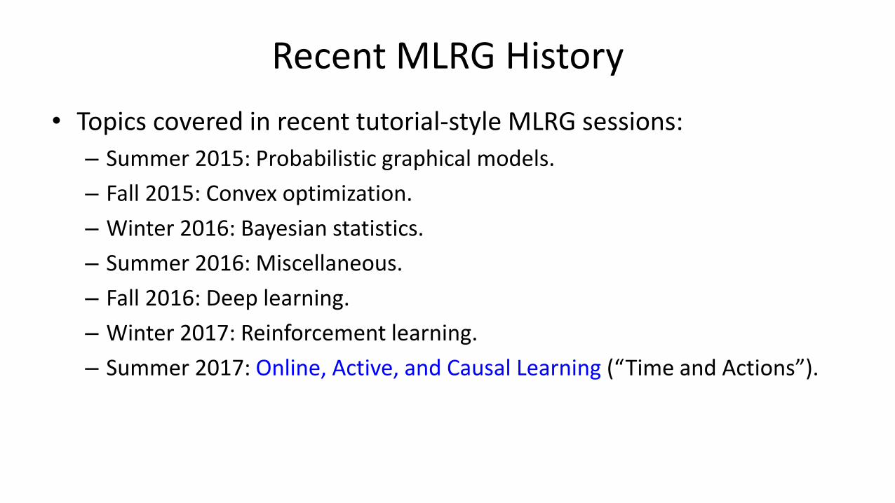
• Topics covered in recent tutorial-style MLRG sessions:
– Summer 2015: Probabilistic graphical models.
– Fall 2015: Convex optimization.
– Winter 2016: Bayesian statistics.
– Summer 2016: Miscellaneous.
– Fall 2016: Deep learning.
– Winter 2017: Reinforcement learning.
– Summer 2017: Online, Active, and Causal Learning (“Time and Actions”).
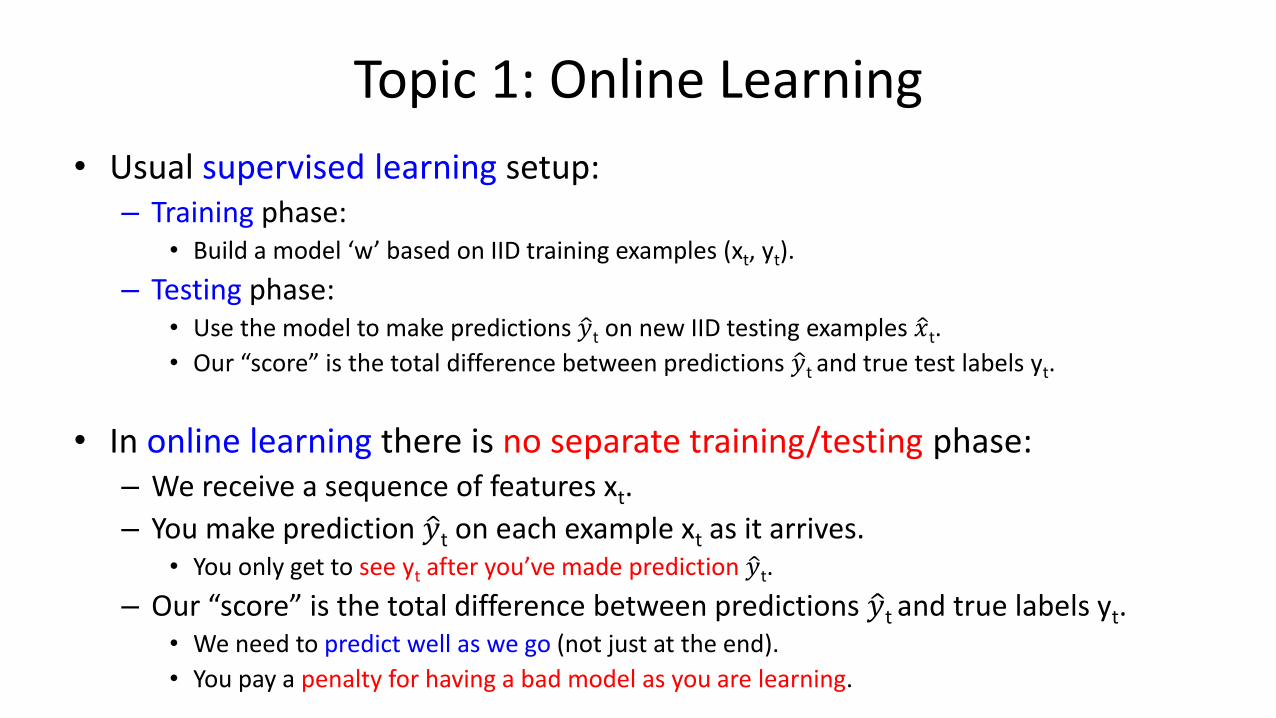
Topic 1: Online Learning
• Usual supervised learning setup: – Training phase:
• Build a model ‘w’ based on IID training examples (xt, yt).
– Testing phase: • Use the model to make predictions 𝑦 t on new IID testing examples 𝑥 t.
• Our “score” is the total difference between predictions 𝑦 t and true test labels yt.
• In online learning there is no separate training/testing phase: – We receive a sequence of features xt.
– You make prediction 𝑦 t on each example xt as it arrives. • You only get to see yt after you’ve made prediction 𝑦 t.
– Our “score” is the total difference between predictions 𝑦 t and true labels yt.
• We need to predict well as we go (not just at the end).
• You pay a penalty for having a bad model as you are learning.
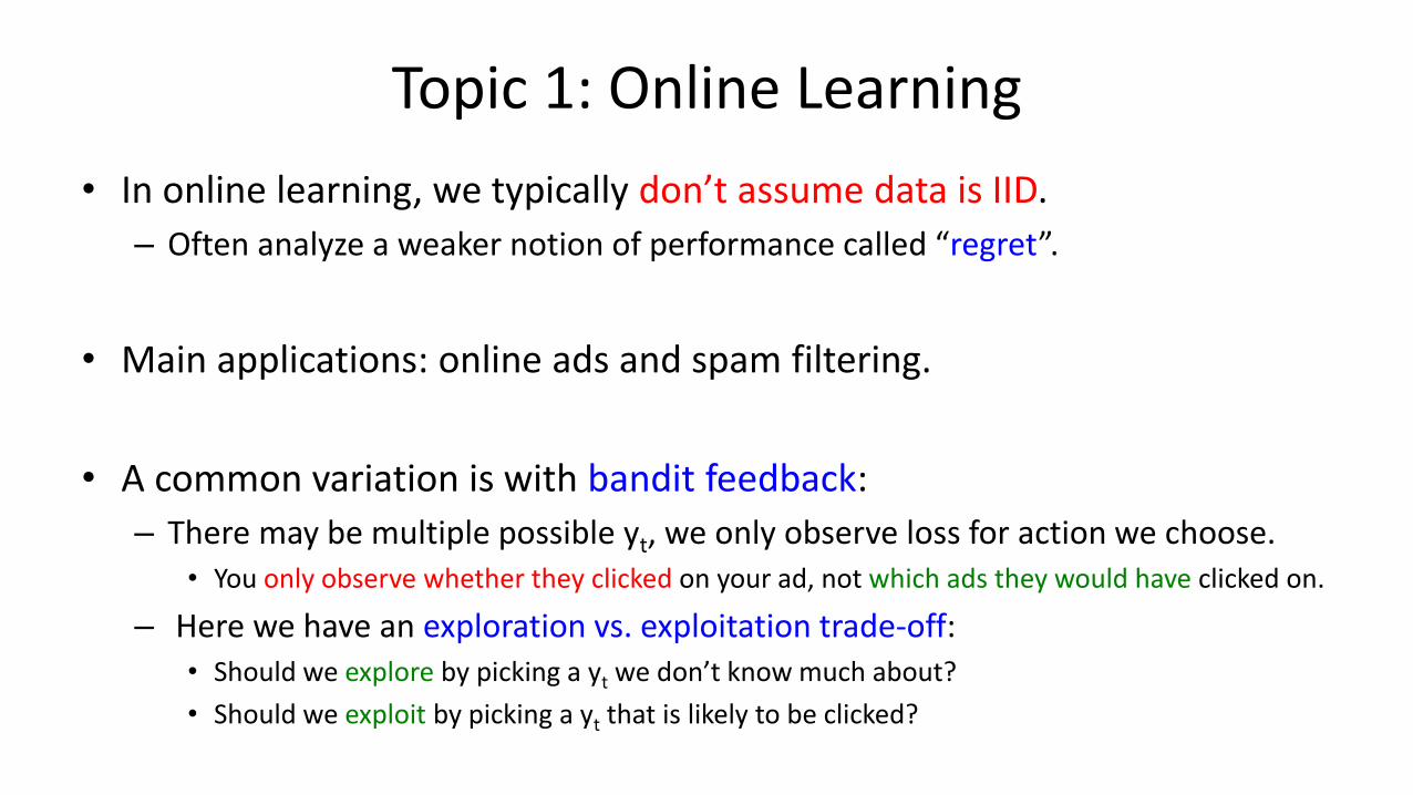
Topic 1: Online Learning
• In online learning, we typically don’t assume data is IID.
– Often analyze a weaker notion of performance called “regret”.
• Main applications: online ads and spam filtering.
• A common variation is with bandit feedback:
– There may be multiple possible yt, we only observe loss for action we choose. • You only observe whether they clicked on your ad, not which ads they would have clicked on.
– Here we have an exploration vs. exploitation trade-off: • Should we explore by picking a yt we don’t know much about?
• Should we exploit by picking a yt that is likely to be clicked?
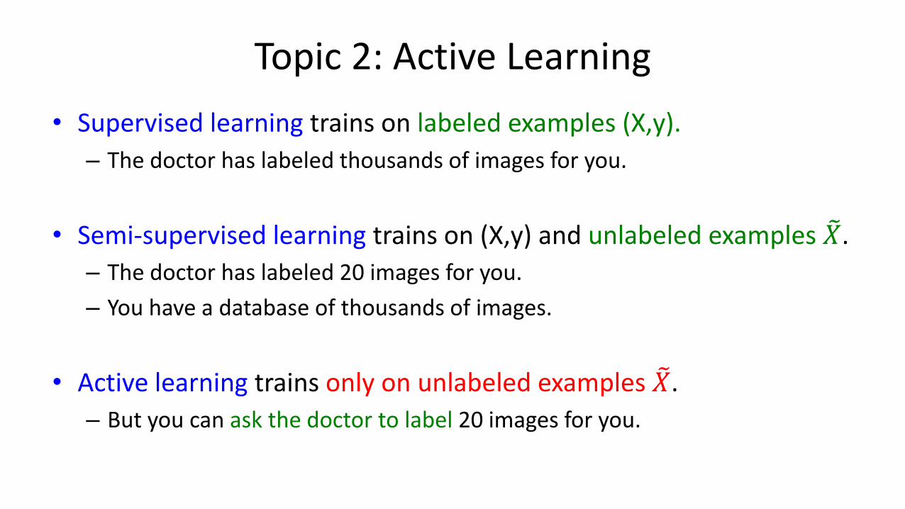
Topic 2: Active Learning
• Supervised learning trains on labeled examples (X,y).
– The doctor has labeled thousands of images for you.
• Semi-supervised learning trains on (X,y) and unlabeled examples 𝑋 .
– The doctor has labeled 20 images for you.
– You have a database of thousands of images.
• Active learning trains only on unlabeled examples 𝑋 .
– But you can ask the doctor to label 20 images for you.
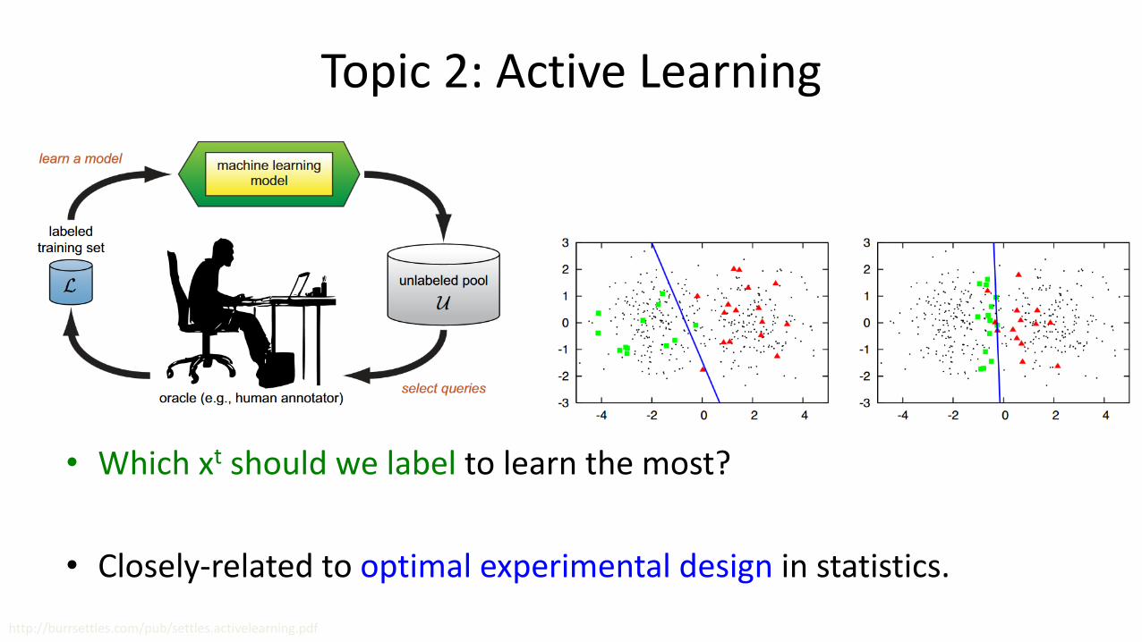
Topic 2: Active Learning
• Which xt should we label to learn the most?
• Closely-related to optimal experimental design in statistics.
http://burrsettles.com/pub/settles.activelearning.pdf
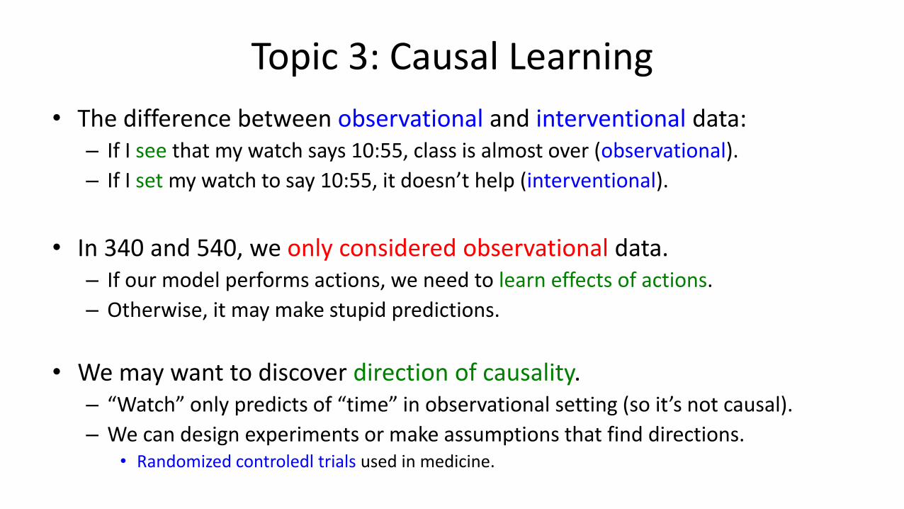
Topic 3: Causal Learning
• The difference between observational and interventional data: – If I see that my watch says 10:55, class is almost over (observational).
– If I set my watch to say 10:55, it doesn’t help (interventional).
• In 340 and 540, we only considered observational data. – If our model performs actions, we need to learn effects of actions.
– Otherwise, it may make stupid predictions.
• We may want to discover direction of causality. – “Watch” only predicts of “time” in observational setting (so it’s not causal).
– We can design experiments or make assumptions that find directions. • Randomized controledl trials used in medicine.
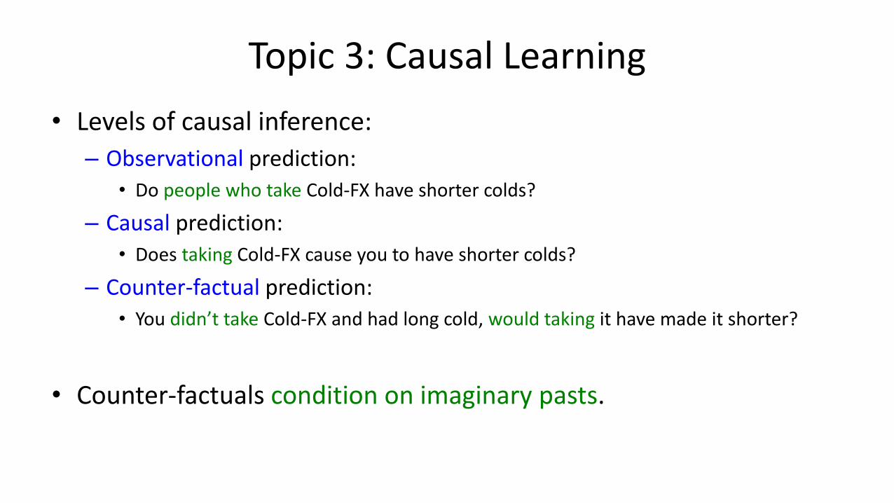
Topic 3: Causal Learning
• Levels of causal inference:
– Observational prediction:
• Do people who take Cold-FX have shorter colds?
– Causal prediction:
• Does taking Cold-FX cause you to have shorter colds?
– Counter-factual prediction:
• You didn’t take Cold-FX and had long cold, would taking it have made it shorter?
• Counter-factuals condition on imaginary pasts.
(pause)
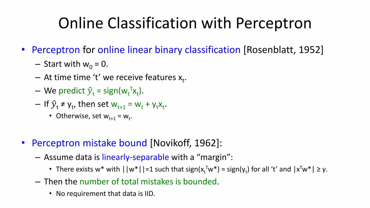
Online Classification with Perceptron
• Perceptron for online linear binary classification [Rosenblatt, 1952]
– Start with w0 = 0.
– At time time ‘t’ we receive features xt.
– We predict 𝑦 t = sign(wtTxt).
– If 𝑦 t ≠ yt, then set wt+1 = wt + ytxt. • Otherwise, set wt+1 = wt.
• Perceptron mistake bound [Novikoff, 1962]:
– Assume data is linearly-separable with a “margin”: • There exists w* with ||w*||=1 such that sign(xt
Tw*) = sign(yt) for all ‘t’ and |xTw*| ≥ γ.
– Then the number of total mistakes is bounded. • No requirement that data is IID.
Perceptron Mistake Bound
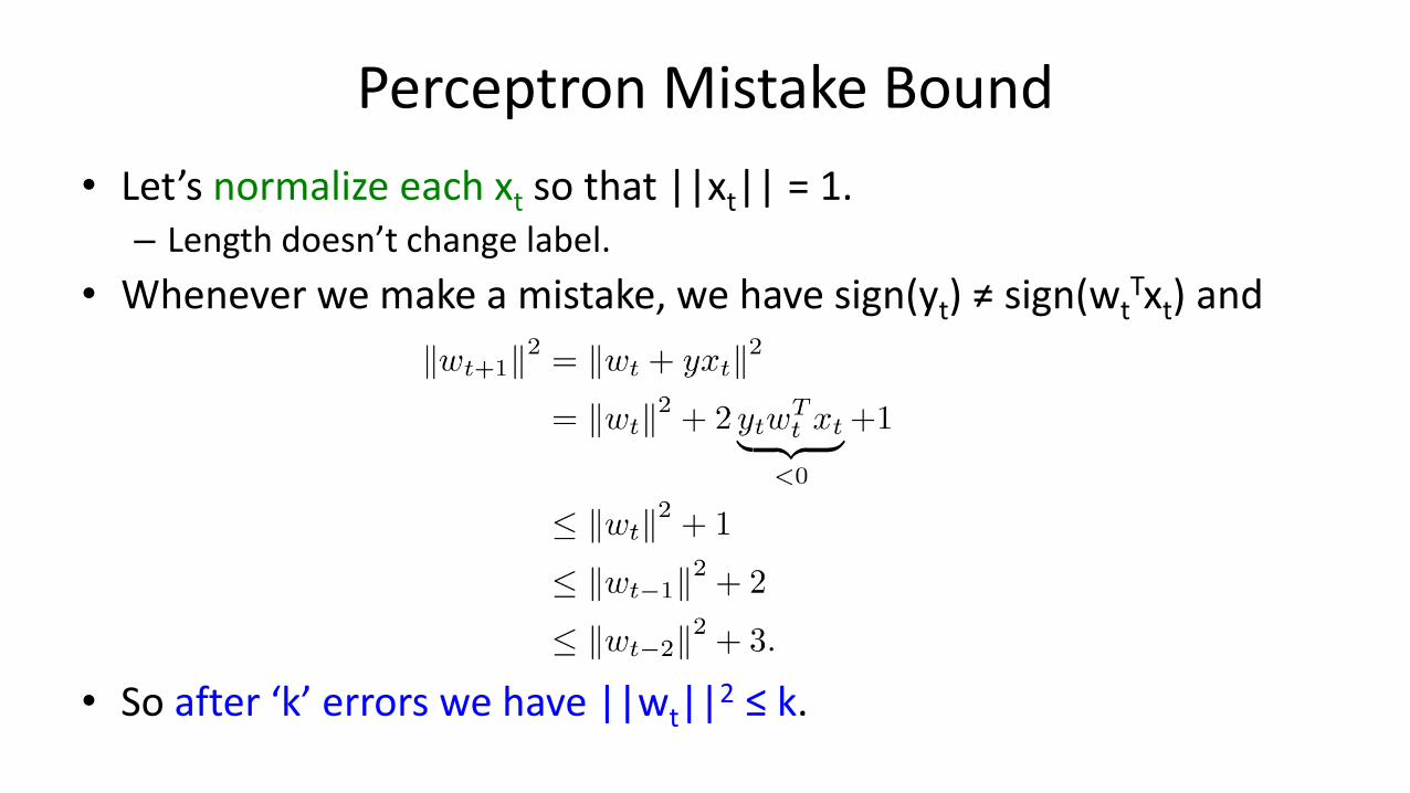
• Let’s normalize each xt so that ||xt|| = 1. – Length doesn’t change label.
• Whenever we make a mistake, we have sign(yt) ≠ sign(wtTxt) and
• So after ‘k’ errors we have ||wt||2 ≤ k.
Perceptron Mistake Bound
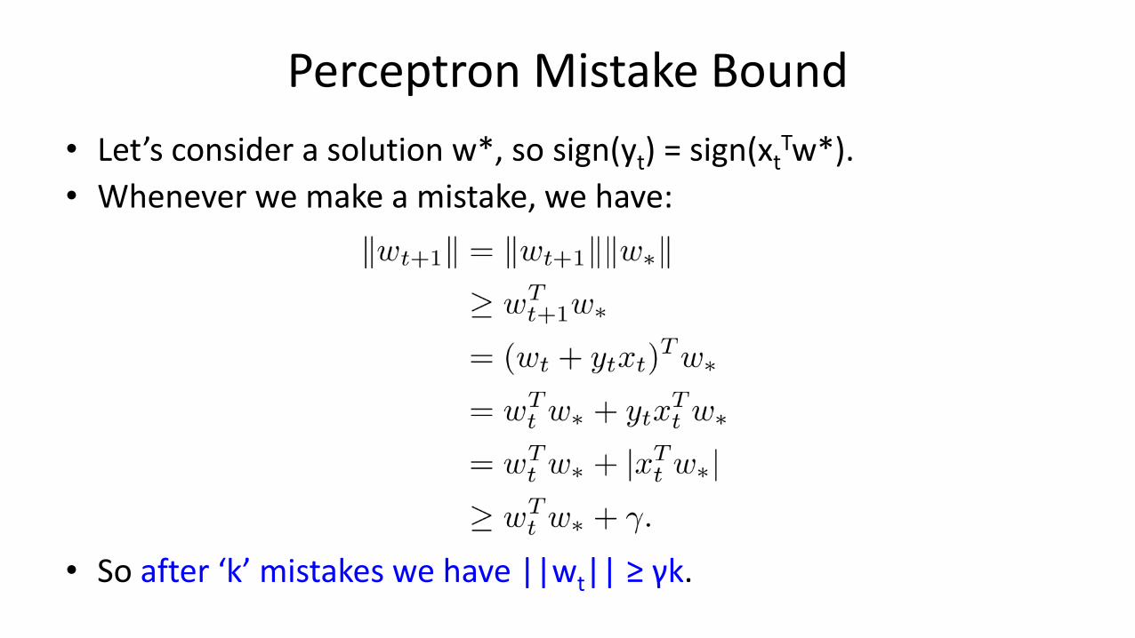
• Let’s consider a solution w*, so sign(yt) = sign(xtTw*).
• Whenever we make a mistake, we have:
• So after ‘k’ mistakes we have ||wt|| ≥ γk.
Perceptron Mistake Bound
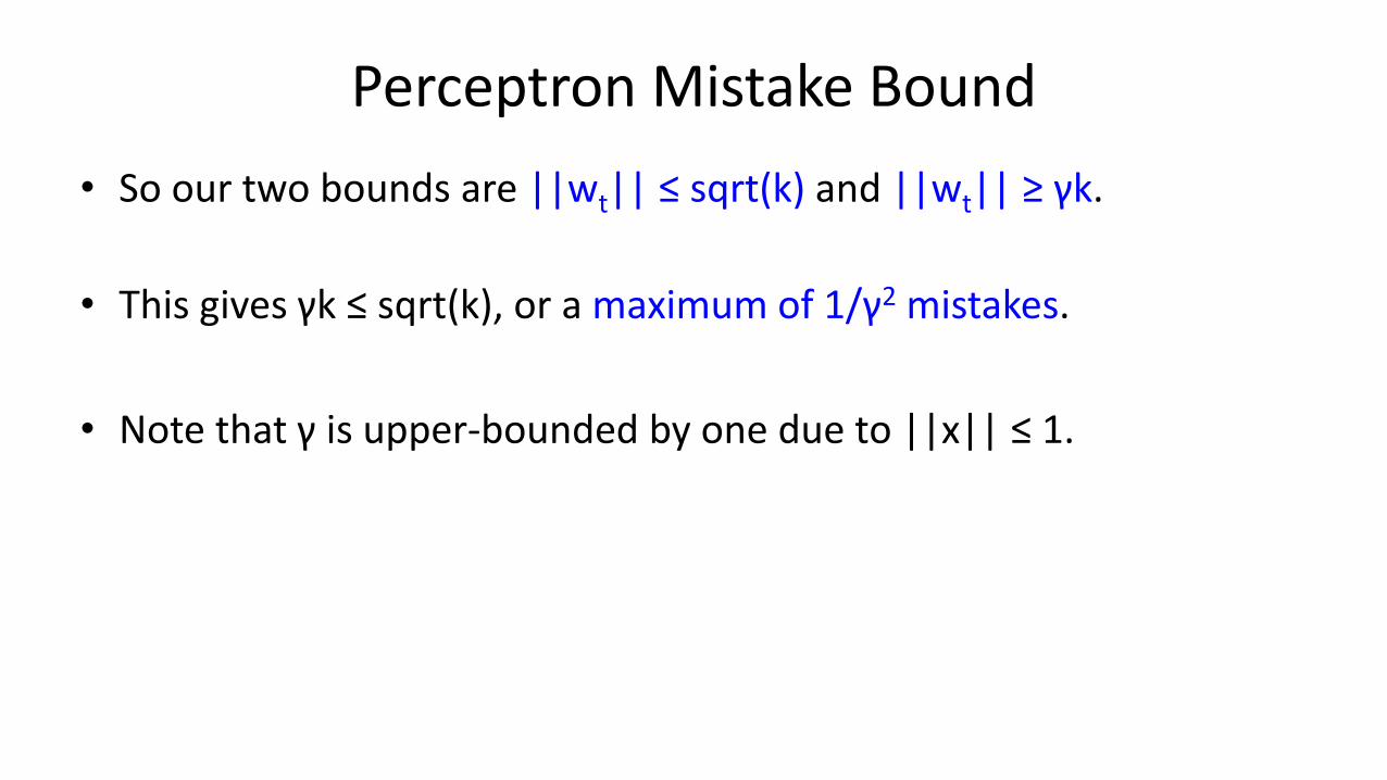
• So our two bounds are ||wt|| ≤ sqrt(k) and ||wt|| ≥ γk.
• This gives γk ≤ sqrt(k), or a maximum of 1/γ2 mistakes.
• Note that γ is upper-bounded by one due to ||x|| ≤ 1.
Beyond Separable Problems: Follow the Leader
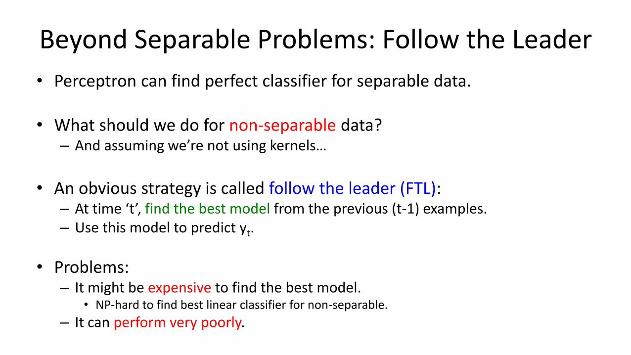
• Perceptron can find perfect classifier for separable data.
• What should we do for non-separable data? – And assuming we’re not using kernels…
• An obvious strategy is called follow the leader (FTL):
– At time ‘t’, find the best model from the previous (t-1) examples. – Use this model to predict yt.
• Problems: – It might be expensive to find the best model.
• NP-hard to find best linear classifier for non-separable.
– It can perform very poorly.
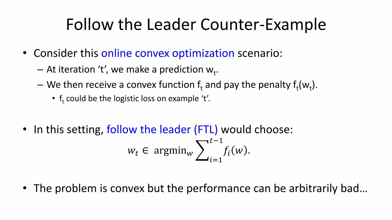
Follow the Leader Counter-Example
• Consider this online convex optimization scenario:
– At iteration ‘t’, we make a prediction wt.
– We then receive a convex function ft and pay the penalty ft(wt).
• ft could be the logistic loss on example ‘t’.
• In this setting, follow the leader (FTL) would choose:
𝑤𝑡 ∈ argmin𝑤 𝑓𝑖 𝑤 .𝑡−1
𝑖=1
• The problem is convex but the performance can be arbitrarily bad…
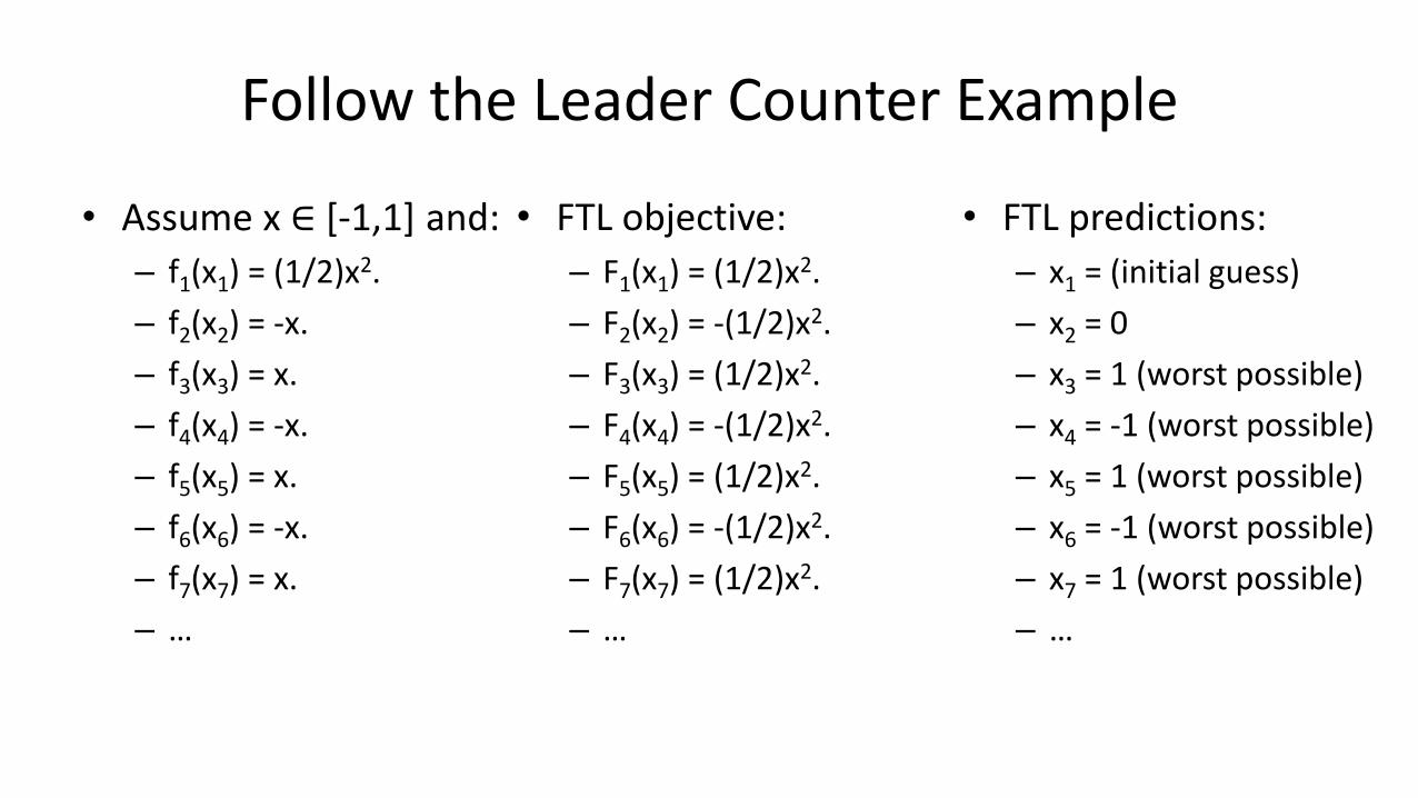
Follow the Leader Counter Example
• Assume x ∈ [-1,1] and:
– f1(x1) = (1/2)x2.
– f2(x2) = -x.
– f3(x3) = x.
– f4(x4) = -x.
– f5(x5) = x.
– f6(x6) = -x.
– f7(x7) = x.
– …
• FTL predictions:
– x1 = (initial guess)
– x2 = 0
– x3 = 1 (worst possible)
– x4 = -1 (worst possible)
– x5 = 1 (worst possible)
– x6 = -1 (worst possible)
– x7 = 1 (worst possible)
– …
• FTL objective:
– F1(x1) = (1/2)x2.
– F2(x2) = -(1/2)x2.
– F3(x3) = (1/2)x2.
– F4(x4) = -(1/2)x2.
– F5(x5) = (1/2)x2.
– F6(x6) = -(1/2)x2.
– F7(x7) = (1/2)x2.
– …
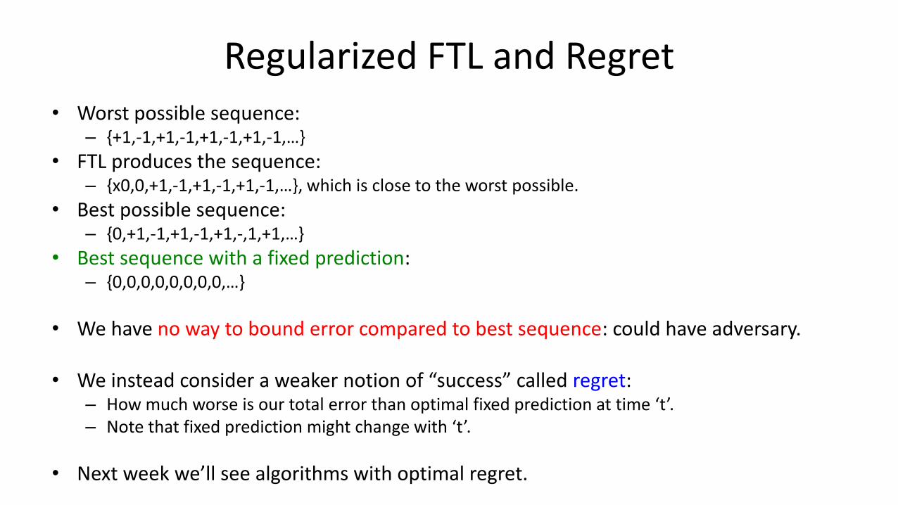
Regularized FTL and Regret • Worst possible sequence:
– {+1,-1,+1,-1,+1,-1,+1,-1,…}
• FTL produces the sequence: – {x0,0,+1,-1,+1,-1,+1,-1,…}, which is close to the worst possible.
• Best possible sequence: – {0,+1,-1,+1,-1,+1,-,1,+1,…}
• Best sequence with a fixed prediction: – {0,0,0,0,0,0,0,0,…}
• We have no way to bound error compared to best sequence: could have adversary.
• We instead consider a weaker notion of “success” called regret: – How much worse is our total error than optimal fixed prediction at time ‘t’. – Note that fixed prediction might change with ‘t’.
• Next week we’ll see algorithms with optimal regret.
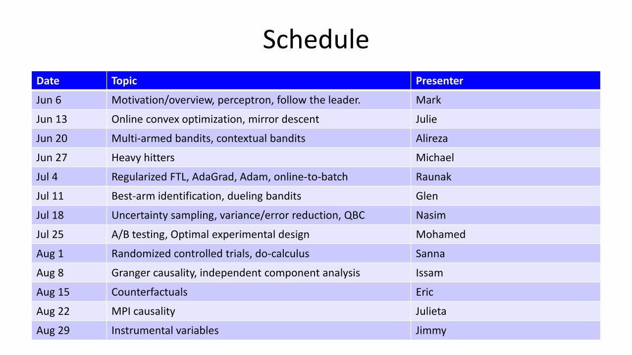
Schedule Date Topic Presenter
Jun 6 Motivation/overview, perceptron, follow the leader. Mark
Jun 13 Online convex optimization, mirror descent Julie
Jun 20 Multi-armed bandits, contextual bandits Alireza
Jun 27 Heavy hitters Michael
Jul 4 Regularized FTL, AdaGrad, Adam, online-to-batch Raunak
Jul 11 Best-arm identification, dueling bandits Glen
Jul 18 Uncertainty sampling, variance/error reduction, QBC Nasim
Jul 25 A/B testing, Optimal experimental design Mohamed
Aug 1 Randomized controlled trials, do-calculus Sanna
Aug 8 Granger causality, independent component analysis Issam
Aug 15 Counterfactuals Eric
Aug 22 MPI causality Julieta
Aug 29 Instrumental variables Jimmy